Min-type Morse theory for configuration spaces of hard spheres

Abstract.

In this paper we study configuration spaces of hard spheres in a bounded region. We develop a general Morse-theoretic framework and show that mechanically balanced configurations play the role of critical points. As an application, we find the precise threshold radius for a configuration space to be homotopy equivalent to the configuration space of points.

1. Introduction

Configuration spaces of $n$ points in ${\mathbb{R}}^{d}$ are well studied [4]. In this article we are interested in a natural generalization, configuration spaces of non-overlapping balls in a bounded region in ${\mathbb{R}}^{d}$.

Besides their intrinsic mathematical interest, the study of these spaces is motivated by physical considerations. For example, in statistical mechanics “hard spheres” (or in two dimensions “hard disks”) are among the most well-studied models of matter. Computer simulations suggest a solid-liquid phase transition for hard spheres [17], but this is not well understood mathematically.

A number of papers in statistical mechanics have explored the hypothesis that underpinning phase transitions are changes in the topology of the underlying configuration space or equipotential submanifolds [24, 16, 1, 9]. Franzosi, Pettini, and Spinelli show that under fairly general conditions (smooth, finite-range, confining potentials), the Helmholtz free energy cannot pass through a phase transition unless there is a change in the topology of the underlying configuration space [11, 10]. This theorem unfortunately does not apply to configuration spaces of hard spheres, since the potential function is not smooth — but the Morse-theoretic methods developed here may be a step in the direction of extending it to include hard spheres.

Several other papers have investigated configuration spaces as models of motion planning for robots [8, 13]. For example, Farber’s “topological complexity” can be thought of as measuring the difficulty of designing an algorithm for navigating the space. As Deeley recently pointed out when he studied “thick particles” on metric graphs, the assumption that robots are points is not physically realistic, and giving the points thickness wildly complicates the topology of the underlying configuration space [6].

Let ${\mathcal{B}}$ be a bounded region in ${\mathbb{R}}^{d}$. Define ${{\mathtt{Conf}}}(n,r)$ to be the configuration space of $n$ non-overlapping balls of radius $r$ in ${\mathcal{B}}$. We are especially interested here in understanding when the topology changes if $n$ is fixed and $r$ is varying . First we consider the extreme cases. For $r$ sufficiently small, one expects that ${{\mathtt{Conf}}}(n,r)$ is homotopy equivalent to the configuration space ${\mathtt{Conf}}(n)$ of $n$ distinct points in ${\mathcal{B}}$ — for a survey of configuration spaces of points see Cohen [4]. On the other hand for $r$ sufficiently large, ${{\mathtt{Conf}}}(n,r)$ is empty. Indeed finding the smallest such $r$ is the sphere packing problem in a bounded region — see for example Graham et al. [15, 2, 18, 19] and Melissen [22, 21].

In this note we develop a Morse-theoretic framework which provides a necessary condition for the topology to change — mechanical balanced configurations play the role of critical points (and submanifolds). As an illustration of the method, we find the precise threshold radius below which ${\mathtt{Conf}}(n,r)$ is homotopy equivalent to ${\mathtt{Conf}}(n)$.

2. Tautological Morse function

Fix $n$, and define ${\mathtt{Conf}}(n)$ to be the set of ordered $n$-tuples of distinct points in a bounded domain ${\mathcal{B}}\subset{\mathbb{R}}^{d}$:

$${\mathtt{Conf}}(n)=\{{\vec{x}}=(x_{1},\ldots,x_{n})\mid x_{i}\in{\mathcal{B}},x_{i}\neq x_{j}\text{ for }i\neq j\}.$$

As an open subset of ${\mathbb{R}}^{dn}$, ${\mathtt{Conf}}(n)$ has the structure of a smooth manifold. Let ${\mathbf{\tau}}:{\mathtt{Conf}}(n)\to{\mathbb{R}}$ be defined by

(1) $${\mathbf{\tau}}({\vec{x}}):=\min\left(\frac{1}{2}\min_{i\neq j}d(x_{i},x_{j}),\min_{i}\min_{p\in\partial{\mathcal{B}}}d(x_{i},p)\right),$$

where $\partial{\mathcal{B}}$ denotes the boundary of ${\mathcal{B}}$. We call $\tau$ the tautological function. Then by definition the configuration space of $n$ balls of radius $r$ in ${\mathcal{B}}$ is given by

$${{\mathtt{Conf}}}(n,r)={\mathbf{\tau}}^{-1}[r,\infty).$$

This observation suggests using a “Morse”-type theory of ${\mathbf{\tau}}$ to study the topology of ${{\mathtt{Conf}}}(n,r)$ and especially how the topology changes as $r$ varies. One obvious trouble on that route is the fact that ${\mathbf{\tau}}$ typically is not smooth, so that we need a general framework which allows us to work with non-smooth functions.

In the next section we will discuss the properties of min-type functions, that is functions on a manifold $M$ given as the minimum of a parametric family of real valued functions

$${\mathbf{\tau}}(x):=\min_{p}f(p,x),x\in M,p\in P,$$

where $P$ is a compact parameter space, and $f$ is continuously differentiable in $x$ for every fixed $p\in P$. We note that the function given by (1) falls within this category, if one considers as $P$ the disjoint union of the discrete set corresponding to pairs $(i,j),1\leq i<j\leq n$ and of $n$ copies of the boundary, formed by the pairs $(i,p),1\leq i\leq n,p\in\partial{\mathcal{B}}$.

It should be remarked that the Morse-type theory of the min (or even min-max) type functions has appeared in the literature (compare [20, 3, 12]), but in a much more restrictive context (with essentially finite parameter space).

3. Min-type Morse theory

Let us start with some notation and definitions.

For a manifold $M$ and function $f:M\to{\mathbb{R}}$, let $M^{c}$ denote the superlevel set at $c$, i.e. $M^{c}=f^{-1}[c,\infty)$.

We say that a function $h:(s,t)\to{\mathbb{R}}$, is increasing with speed at least $v>0$ if $h(t^{\prime})-h(s^{\prime})\geq v(t^{\prime}-s^{\prime})$ for any $s^{\prime}<t^{\prime}$ in the interval $(s,t)$. We note that such a function does not have to be even continuous.

We record for later use the following (immediate) result:

Lemma 3.1.

Let $f:M\times{\mathbb{R}}\to{\mathbb{R}}$ be a continuous proper function, (strictly) increasing along each fiber $\{x\}\times{\mathbb{R}}$. Then the fiber-wise inverse $\phi:(x,c)\mapsto\inf(t:f(x,t)=c)$ is continuous on $M\times[c_{1},c_{2}]$ for any interval $[c_{1},c_{2}]$ which belongs to the ranges of all the functions $f_{x}(\cdot):=f(x,\cdot)$.

Proof.

As $f$ is proper, then the $t$-projection of the preimage of a compact interval $[c_{1},c_{2}]$ is compact as well. Further, if a sequence $(x_{i},c_{i})$ converges to $(x_{*},c_{*})$, yet $t_{i}:=\phi(x_{i},c_{i})$ fails to converge to $t_{*}:=\phi(x_{*},c_{*})$, we can, using the boundedness of the sequence $(t_{i})$, choose a subsequence such that along it $t_{j}\to t\neq t_{*}$. By continuity, $\lim f(x_{j},t_{j})=f(x_{*},t)$ (as $x_{j}$ converge to $x_{*}$). The fact that $f(x_{j},t_{j})=c_{j}$ implies that $f(x_{*},t)$ equals $c_{*}$, which by the continuity of $f$ also equals $f(x_{*},t_{*})$. This contradicts the assumption that $f$ increases fiber-wise. ∎

For a smooth vector field $V$ on $M$ we will denote the time $t$ shift along the trajectories of $V$ as $S_{t}^{V}$. We will say that the function $f$ increases along the trajectories of $V$ with non-zero speed, if for some common $v>0$, and for all $x\in M$, $h_{x}:t\mapsto f(S^{V}_{t}x)$ increases with speed at least $v$.

Lemma 3.2.

Let $M$ be a smooth manifold and $f:M\to{\mathbb{R}}$ a continuous function, such that $M^{a}$ is compact. Suppose that $M$ admits a smooth vector field $V$ non-vanishing on $f^{-1}[a,b]$, and such that $f$ is increasing along the trajectories of $V$ on the set $f^{-1}[a,b]$ with non-zero speed. Then $M^{b}$ is a deformation retract of $M^{a}$.

Lemma 3.2 can be seen as a generalization of Theorem 3.1 in [23] for non-smooth functions $f$. We remark here that one can drop here the non-zero speed condition, requiring only that $f$ is increasing along the trajectories of $V$, but we do not need this strengthened form in this paper.

Proof.

For $x\in M^{a}$ set a partially defined function on $M^{a}\times{\mathbb{R}}$ by $g(x,t):=f(S_{t}^{V}x)$. The non-zero speed condition implies that $[a,b]$ is in the range of $g(x,\cdot)$ for any $x\in f^{-1}([a,b])$, and together with the compactness of $M^{a}$ implies that $g$ is proper. Hence, by Lemma 3.1, $\tilde{\phi}(x,c)=\inf(t:f(S_{t}^{V}x)\geq c)$ is well defined and continuous, as well as $\phi(x,c)=\max(\tilde{\phi}(x,c),0)$. As for any $c\leq f(x)$, $\phi(x,c)=0$, $\phi$ vanishes on $M^{b}\times[a,b]$.

Now define the homotopy

$$H:M^{a}\times[0,1]\to M^{a}$$

as

$$H:(x,\tau)\mapsto S^{V}_{\phi(x,(1-\tau)a+\tau b)}x.$$

Continuity of $\phi$ implies continuity of $H$; the facts that $H(x,0)=\mathit{id}_{M^{a}}$, $H(x,\tau)|_{M^{b}}=\mathit{id}_{M^{b}}$ for $0\leq\tau\leq 1$ and $H(x,1)\in M^{b}$ are immediate. ∎

3.1. Regular values of min-type functions

Next we will use the fact that the tautological function ${\mathbf{\tau}}$ is the minimum of a compact family of smooth functions. We want to establish conditions when a value $c$ is topologically regular, that is for which there exists some $\epsilon>0$ such that $M^{c+\epsilon}$ is a deformation retract of $M^{c-\epsilon}$.

We give a general condition for topological regularity, as follows.

Let $P$ be a compact metric space, $M$ a compact smooth manifold with boundary and

$$f:P\times M\to{\mathbb{R}}$$

a continuous function such that the $x$-derivative of $f$ (that is, the gradient of $f_{p}$, where $f_{p}(x)=f(p,x)$) is continuous on $P\times M$. We will be talking of $P$ as the parameter space.

We denote by ${\mathbf{\tau}}:=\min_{p\in P}f_{p}$ the min-function of the family $f$. The set $N\subset P\times M$ defined by

$$N:=\{(p,x):f(p,x)={\mathbf{\tau}}(x)\}$$

is compact, and the slices

$$N_{x}:=\{p\in P:(p,x)\in N\}$$

are upper semi-continuous: for any $x\in M$ and any open neighborhood $UN_{x}\supset N_{x}$ there exists an open neighborhood $Ux\ni x$ such that for $x^{\prime}\in Ux$, $N_{x^{\prime}}\subset UN_{x}$.

Next we show that if one can perturb each $x$ to increase $\tau$ then we can do so globally with a minimum speed.

Lemma 3.3.

Assume that for any $x\in M$, there exists a tangent vector $V_{x}\in T_{x}M$ such that $L_{V_{x}}f_{p}>0$ for all $p\in N_{x}$. Then

• for some positive $v$ there exists smooth vector field $V$ on $M$ such that $L_{V}f_{p}\geq v>0$ in some open vicinity of $N$, and

• along the trajectories of $V$, the min-function ${\mathbf{\tau}}$ increases with speed at least $v$.

Proof.

For any $x\in M$, we can extend the vector $V_{x}\in T_{x}M$ to a smooth vector field on $M$ (which we still denote as $V_{x}$), such that $L_{V_{x}}f>0$ in some open vicinity $UN_{x}\times Ux$ of $N_{x}\times\{x\}$. By compactness, there exists a finite collection of points $\{x_{i}\}$ in $M$ such that the open sets $U_{i}:=UN_{x_{i}}\times Ux_{i}$ cover $N$ (and the open sets $Ux_{i}$ cover $M$), and $v>0$ such that $L_{V_{i}}f_{p}\geq v$ on $U_{i}$ (here $V_{i}:=V_{x_{i}}$). Using a partition of unity we arrive at the first conclusion. The second conclusion is immediate. ∎

For $x\in M$ consider the intersection of the open half-spaces

$$H_{x}(p):=\{v\in T_{x}M:\langle df_{p}|_{x},v\rangle>0\}$$

over all $p\in N_{x}$. This is an open convex cone

$$C^{o}_{x}:=\bigcap_{p\in N_{x}}H_{x}(p)$$

in $T_{x}M$.

Upper semicontinuity of $N_{x}$ implies lower semicontinuity of $C^{o}_{x}$; for any $x\in M$ and any open set $V\subset TM$ intersecting $C^{o}_{x}$, there exists an open neighborhood $Ux\ni x$ such that for $x^{\prime}\in Ux$, $C^{o}_{x^{\prime}}$ intersects $V$. In particular, if $C^{o}_{x}$ is non-empty, it remains such in a vicinity of $x$.

Combining Lemmata 3.2 and 3.3 we obtain the following

Corollary 3.4.

If the cones $C^{o}_{x}$ are non-empty over the level set ${\mathbf{\tau}}^{-1}(c)$, then $c$ is topologically regular.

For general min-type functions this is essentially the best possible condition for the regularity of the critical values. If the functions $f_{p}$ are quasi-convex, i.e. have convex lower excursion sets $\{f_{p}\leq c\}$, then Corollary 3.4 can be considerable strengthened. Thus, one can show (we will do it in a follow-up paper) that a critical value is topologically regular, if for all points at the level set, the intersection of the closed half-spaces is a cone over a contractible base. This observation relies on stratified Morse theory due to Goresky and MacPherson[14], but is in a nutshell close to the elementary result used by Connelly in his work on the existence of continuous “unlocking” deformations of hard ball configurations, see [5].

Corollary 3.4 implies that unless the level set of the tautological function $\tau^{-1}(r)$ contains a point $x$ with $C^{o}_{x}=\varnothing$, the homotopy type of ${{\mathtt{Conf}}}(n,r)$ is locally constant at $r$.

By Farkas’ lemma, the emptiness of the cone $C^{o}_{x}$ implies that there exists a finite collection of points $p_{i}\in N_{x},i=1,\ldots,I\leq\dim M+1$, and positive weights $w_{i}>0$ such that

(2) $$\sum_{i}w_{i}{df_{p_{i}}|_{x}}=0.$$

4. Critical points and stress graphs

In our hard spheres setting, the vanishing of the convex combination (2) has a clear geometric interpretation.

For ${\vec{x}}\in{\mathtt{Conf}}(n,r)$, define a stress graph of ${\vec{x}}$ to be a graph embedded in ${\mathbb{R}}^{d}$ whose vertices are the points $x_{1},\ldots,x_{n}$ and boundary points $y\in{\partial}{\mathcal{B}}$ where $d(x_{i},y)=r$ for some $i$. The edges are the pairs $\{x_{i},x_{j}\}$ where $d(x_{i},x_{j})=2r$ and $\{x_{i},y\}$ where $d(x_{i},y)=r$. Each edge $k$ is assigned a positive weight $w_{k}$. The points $x_{i}$ are referred to as internal points and the points $y$ are referred to as boundary points. We interpret this graph as a system of mechanical stresses, with (repulsive) forces acting on the endpoints of a segment $k$ equal to $w_{k}$ times the unit vector in the direction of $k$. Call the mechanical stresses acting on boundary points boundary mechanical stresses. Call a connected component trivial if it consists of a single point. Call ${\vec{x}}$ trivial if $\Gamma({\vec{x}})$ has no edges.

A stress graph is said to be balanced if it satisfies the following condition.

• The mechanical stresses at each internal point sum to zero.

• The boundary mechanical stresses on each connected component sum to zero.

Say that the configuration is ${\vec{x}}$ is balanced if it has a balanced stress graph.

Call an internal point isolated if it is not in the boundary of any edges. For each point $x_{i}$ call the intersection of the stress graph with the points on the sphere $d(x_{i},x)=r$ kissing points of $x_{i}$. Call a kissing point that is also a boundary point a boundary kissing point.

Lemma 4.1.

Assume that ${\vec{x}}\in{\mathtt{Conf}}(n,r)$ is balanced. Then

1. each non-isolated internal point is in the convex hull of its kissing points, and

2. each non-trivial connected component is contained in the convex hull of its boundary kissing points.

Now consider ${\vec{x}}\in{\mathtt{Conf}}(n)$ that is a critical point of $\tau$ with critical value $r$. In (2), the parameters $p_{i}$ correspond either to the pairs of touching hard spheres, $d(x_{a_{i}},x_{b_{i}})=2r$, or to the hard sphere $x_{c_{i}}$ touching the boundary, $d(x_{c_{i}},y_{i})=r$, at a point $y_{i}\in\partial{\mathcal{B}}$. Let $\Gamma({\vec{x}})$ be the corresponding stress graph for ${\vec{x}}$ with weights given by the coefficients $w_{i}$ in (2).

Theorem 4.2.

If ${\vec{x}}\in{\mathtt{Conf}}(n)$ is a critical point of $\tau$ with critical value $r$, then ${\vec{x}}$ is balanced and nontrivial as a point in ${\mathtt{Conf}}(n,r)$.

Proof.

Consider ${\vec{x}}\in{\mathtt{Conf}}(n,r)$ and consider $\Gamma({\vec{x}})$. From (2) it follows that the mechanical stresses at each internal point sum to zero.

The sum of mechanical stresses in each connected component equals the sum of mechanical stresses on internal points and the sum of external mechanical stresses. From (2) and the first observation it follows that the boundary mechanical stresses on each connected component sum to zero.

Finally, since the sum in (2) is nontrivial, ${\vec{x}}$ is nontrivial. ∎

5. Hard spheres in a box

Consider now in more detail the case of hard spheres in a rectangular box with sides $L:=L_{1}\leq\ldots\leq L_{d}$, given, for definitiveness sake, by

$${\mathcal{B}}=\{0\leq f_{m}\leq L_{m},m=1,\ldots,d\}.$$

(Here $\{f_{m}\}$ is the orthonormal coordinate system on ${\mathbb{R}}^{d}$.)

5.1. Initial interval

We show that Theorem 4.2 implies a lower bound on the length of the initial interval of values of $r$, where the homotopy type of ${{\mathtt{Conf}}}(n,r)$ remains constant.

Theorem 5.1.

For the rectangular box ${\mathcal{B}}$, there are no critical values of ${\mathbf{\tau}}$ in $(0,L/2n)$, and therefore,

$${{\mathtt{Conf}}}(n,r)\simeq{\mathtt{Conf}}(n)$$

for $r<L/2n$.

Proof.

Assume that ${\vec{x}}\in{\mathtt{Conf}}(n)$ is a critical value for $\tau$ with critical value $r$. Then by Theorem 4.2, ${\vec{x}}$ is balanced and nontrivial. A connected component of $\Gamma({\vec{x}})$ contains at most $n$ internal points and thus has diameter at most $2nr$. Since ${\vec{x}}$ is nontrivial, it has at least one nontrivial connected component. It is contained in the convex hull of its boundary points, so it contains at least one boundary point. Since the boundary mechanical stresses of this connected component sum to zero, it must contain a pair of boundary points from opposing faces. Thus the diameter of this connected component is at least $L$. Therefore $r\geq L/2n$. ∎

We remark that the balanced stress graph of minimal diameter is not necessarily a segment, for non-rectangular boxes. For example, for the “concave triangle”, it is a cone over three points, see Figure 1.

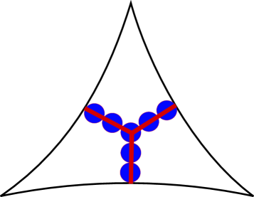
Figure 1. Minimal length stress graph

5.2. First perestroika

A natural question is now to ask, whether there is a topology change as $nr$ goes above the minimal length of the stress graph. We concentrate in the rest of the note on the case of the rectangular box with the shortest side of length $L$, and will investigate, whether

$$i:{{\mathtt{Conf}}}(n,r^{\prime})\to{{\mathtt{Conf}}}(n,r),r^{\prime}=L/2n+\epsilon,r=L/2n-\epsilon$$

is a homotopy equivalence, for small enough $\epsilon$.

We argue that it is not, by presenting explicit nontrivial $(dn-n-d)$-cycles in $\ker(Hi)\subset H_{dn-n-d}({{\mathtt{Conf}}}(n,r^{\prime}),{\mathbb{Z}})$.

Indeed, let $0<\epsilon<L/2n(n-1)$ (so that $(n-1)$ disks of radius $r^{\prime}$ would fit within the box when arranged in a vertical column, and $n$ would not), and consider the set $S_{\epsilon}$ of $n$-point configurations in ${\mathcal{B}}$ given by the conditions

• $x_{1}$ fixed is at distance $r^{\prime}$ from the center of the face $\{f_{1}=0\}$,

• $|x_{i+1}-x_{i}|=2r^{\prime}$ for $i=1,\ldots n-1$, and

• $x_{n}$ is at distance $r^{\prime}$ from the face $\{f_{1}=L_{1}\}$.

In other words, we consider the configurations for which the $n$ disks touch each other and the opposite horizontal faces, forming a chain, see Figure 2.

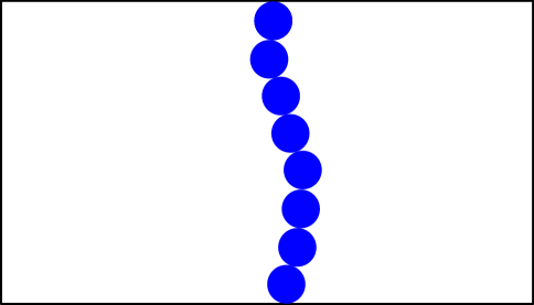
Figure 2. A configuration in $S_{\epsilon}$.

An immediate computation shows that $S_{\epsilon}$ is diffeomorphic to a $(nd-n-d)$-dimensional sphere. Orient it in some way, obtaining a class $s\in H_{nd-n-d}({{\mathtt{Conf}}}(n,r^{\prime}))$.

Next we show that $s$ is nontrivial by constructing a cohomology class with which it has a nontrivial pairing.

Consider now the set $\Sigma$ of configurations in ${\mathcal{B}}^{n}$ given by

• all points $x_{1},\ldots,x_{n}$ have the same coordinates $f_{3},\ldots,f_{d}$;

• all points $x_{2},\ldots,x_{n}$ have the same coordinates $f_{2},\ldots,f_{d}$;

• the $f_{1}$ coordinates of $x_{2},\ldots,x_{n}$ satisfy

  $$f_{1}(x_{1})\geq r;f_{1}(x_{i+1})-f_{1}(x_{i})\geq 2r,\mathrm{for\,}i=2,\ldots,n-1;f_{1}(x_{n})\leq L-r,$$

  and

• $f_{2}(x_{1})\leq f_{2}(x_{2})$.

In other words, the configuration consists of $n-1$ vertically aligned nonoverlapping $r$-disks constrained to have the same $(f_{1},f_{2})$-plane (with the same $f_{3},\ldots_{d}$ coordinates as the disk $x_{1}$), see Figure 3.

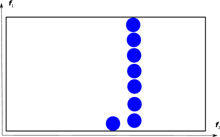
Figure 3. A configuration in $\Sigma$.

The conditions above are given by a finite collection of linear equalities and inequalities, and therefore define a convex polyhedron of dimension $d+n$. The boundary of this polyhedron is in ${\mathcal{B}}^{n}-{{\mathtt{Conf}}}(n,r^{\prime})$, whence, upon orientation it defines a relative class $\sigma\in H_{n+d}({\mathcal{B}}^{n},{\mathcal{B}}^{n}-{{\mathtt{Conf}}}(n,r^{\prime}))$.

We notice that the space ${\mathcal{B}}^{n}$ of $n$-tuples of points in ${\mathcal{B}}$ can be embedded into the $nd$-dimensional sphere $S^{nd}$ (consider a large ball containing ${\mathcal{B}}^{n}$ and contract its boundary to a point). By excision and the long exact sequence for a pair, $H_{n+d}({\mathcal{B}}^{n},{\mathcal{B}}^{n}-{{\mathtt{Conf}}}(n,r^{\prime}))\cong H_{n+d}(S^{nd},S^{nd}-{{\mathtt{Conf}}}(n,r^{\prime}))\cong H_{n+d-1}(S^{nd}-{\mathtt{Conf}}(n,r^{\prime}))$. By Alexander duality the class $\sigma$ can be identified with a class (which we still denote by $\sigma$) in $H^{nd-n-d}({{\mathtt{Conf}}}(n,r^{\prime}))$.

Lemma 5.2.

The pairing between the classes $s$ and $\sigma$ is non-trivial: $s\cdot\sigma=\pm 1$.

Proof.

Indeed, the manifolds $S_{\epsilon}$ and $\Sigma$ intersect transversally at a single point. ∎

As one can observe, there exists a retraction of $S_{\epsilon}$ to a point staying within ${{\mathtt{Conf}}}(n,r)$, implying that the class $s$ is in the kernel of $Hi$. Indeed, we first can reduce all the distances between by shrinking the differences between the adjacent chain centers so that

$$x_{i+1}-x_{i}\mapsto\frac{tr-(1-t)r^{\prime}}{r^{\prime}}(x_{i+1}-x_{i}),t=[0,1];i=1,\ldots,n-1$$

and $x_{1}$ remains fixed (clearly, this homotopy keeps the configuration in ${{\mathtt{Conf}}}(n,r)$). Then one can pull all the vectors $(x_{i+1}-x_{i})$ so that they point vertically upwards (as not one was initially pointing downwards).

For each permutation $\pi$ of indices $1,\ldots,n$ one obtains different classes $s_{\pi}$, and one can easily see that the pairing with the corresponding $n!$ classes $\sigma_{\pi}$ is non-degenerate (because corresponding $S_{\epsilon}$ and $\Sigma$’s are all geometrically distinct). Hence, the rank of the kernel of $Hi$ is at least $n!$.

We notice that the sphericity of the set $S_{\epsilon}$ does not depend on the fact that the stress graph is a chain. For the configuration on Figure 1, the corresponding set is diffeomorphic to a sphere as well: it is just the corollary of the first critical value coming from a topologically Morse critical point, compare [20].

5.3. Betti numbers

We can also compute how the Betti numbers change across the first threshold. Set $r_{*}=L/2n$, and note that as the tautological function is semi-algebraic for semi-algebraic regions, its critical values are isolated. As the only balanced stress graphs in the case of a rectangular domain are the chains spanning the shortest dimension, for some small $\epsilon$ there are no other critical values in $(r_{*}-\epsilon,r_{*}+\epsilon)$.

It is well known [4] that the configuration space ${\mathtt{Conf}}(n)$ of $n$ (labeled) points in ${\mathbb{R}}^{d}$ has Poincaré polynomial

$$P(t) :=\sum_{i\geq 0}\beta_{i}t^{i}$$

$$=\prod_{i=1}^{n-1}\left(1+it^{d-1}\right)$$

$$=1+\dots+(n-1)!H_{n-1}t^{(n-2)(d-1)}+(n-1)!t^{(n-1)(d-1)},$$

where

$$H_{n-1}=\sum_{i=1}^{n-1}1/i.$$

This tells us the Betti numbers of ${\mathtt{Conf}}(n,r_{*}-\epsilon)$, since we have already shown that ${\mathtt{Conf}}(n,r_{*}-\epsilon)$ is homotopy equivalent to ${\mathtt{Conf}}(n)$. We wish to compute the Betti numbers of ${\mathtt{Conf}}(n,r_{*}+\epsilon)$.

Let $N=(n-1)(d-1)$. As we shrink the disks across the critical value $r_{*}=L/2n$, to the configuration space we attach $k\,n!$ cells of dimension $N$, where $k$ is the largest number such that $L_{k}=L$, whose boundaries are representatives for the homology classes $s$ defined in Section 5.2. Each of these cells either increments $\beta_{N}$ or decrements $\beta_{N-1}$.

The first observation is that

$$\beta_{i}[{\mathtt{Conf}}(n,r_{*}+\epsilon)]=\beta_{i}[{\mathtt{Conf}}(n,r_{*}-\epsilon)]$$

for $i\leq N-2$. As (the proof to appear in a follow-up paper) one can show that $\beta_{i}({\mathtt{Conf}}(n,r))=0$ for $i\geq N$ and $r>r_{*}$, so in particular

$$\beta_{i}[{\mathtt{Conf}}(n,r_{*}+\epsilon)]=0$$

for $i\geq N$. Thus $(n-1)!$ of the $N$-cells increase $\beta_{N}$. This leaves only $\beta_{N-1}$ to compute.

Every $N$-cell that does not contribute to $\beta_{N}$ decreases $\beta_{N-1}$. Since we know that $kn!$ cells are added, $(n-1)!$ of them contributing to $\beta_{N}$, we have

$$\beta_{N-1}[{\mathtt{Conf}}(n,r_{*}+\epsilon)]=\beta_{N-1}[{\mathtt{Conf}}(n,r_{*}-\epsilon)]+k\,n!-(n-1)!\;,$$

and since

$$\beta_{N-1}[{\mathtt{Conf}}(n,r_{*}-\epsilon)]=\left\{\begin{array}[]{ll}(n-1)!H_{n-1}&:d=2\\ 0&:d\geq 3,\end{array}\right.$$

we have

$$\beta_{N-1}[{\mathtt{Conf}}(n,r_{*}+\epsilon)]=\left\{\begin{array}[]{ll}(H_{n-1}+kn-1)(n-1)!&:d=2\\ (kn-1)(n-1)!&:d\geq 3.\end{array}\right.$$

6. Concluding remarks

In a future article we will discuss non-degeneracy of critical points, which is closely related to the question of making our necessary condition for a change in the topology sufficient. We also discuss defining and computing the index of critical points, and especially investigate more of the asymptotic properties of ${\mathtt{Conf}}(n,r)$ as $n\to\infty$. In particular we obtain bounds on the rate of growth of Betti numbers.

An important special case for which little seems known is: What is the threshold radius $r=r(n)$ for connectivity of ${\mathtt{Conf}}(n,r)$? This is an important question physically, since for example ergodicity of any Markov process hinges on connectivity of the state space. Diaconis, Lebeau, and Michel noted that $r\leq c/n$ is sufficient to guarantee connectivity of ${\mathtt{Conf}}(n,r)$ [7] and this is best possible for certain regions. It would be interesting to know if connectivity of the configuration space ever extends into the thermodynamic limit, i.e. are there any bounding regions so that ${\mathtt{Conf}}(n,r)$ is connected for $r\leq Cn^{-1/d}$ and some constant $C>0$?

References

- [1] Luca Angelani, Lapo Casetti, Marco Pettini, Giancarlo Ruocco, and Francesco Zamponi. Topology and phase transitions: From an exactly solvable model to a relation between topology and thermodynamics. Phys. Rev. E, 71(3):036152, Mar 2005.
- [2] David W. Boll, Jerry Donovan, Ronald L. Graham, and Boris D. Lubachevsky. Improving dense packings of equal disks in a square. Electron. J. Combin., 7:Research Paper 46, 9 pp. (electronic), 2000.
- [3] L. N. Bryzgalova. The maximum functions of a family of functions that depend on parameters. Funktsional. Anal. i Prilozhen., 12(1):66–67, 1978.
- [4] Frederick R. Cohen. Introduction to configuration spaces and their applications. In Braids, volume 19 of Lect. Notes Ser. Inst. Math. Sci. Natl. Univ. Singap., pages 183–261. World Sci. Publ., Hackensack, NJ, 2010.
- [5] Robert Connelly. Rigidity of packings. European J. Combin., 29(8):1862–1871, 2008.
- [6] Kenneth Deeley. Configuration spaces of thick particles on a metric graph. submitted, 2011.
- [7] Persi Diaconis, Gilles Lebeau, and Laurent Michel. Geometric analysis for the Metropolis algorithm on Lipschitz domains. To appear in Invent. Math.
- [8] Michael Farber. Invitation to topological robotics. Zurich Lectures in Advanced Mathematics. European Mathematical Society (EMS), Zürich, 2008.
- [9] Michael Farber and Viktor Fromm. Homology of planar telescopic linkages. Algebr. Geom. Topol., 10(2):1063–1087, 2010.
- [10] Roberto Franzosi and Marco Pettini. Topology and phase transitions II. Theorem on a necessary relation. Nuclear Physics B, 782(3):219 – 240, 2007.
- [11] Roberto Franzosi, Marco Pettini, and Lionel Spinelli. Topology and phase transitions I. Preliminary results. Nuclear Physics B, 782(3):189 – 218, 2007.
- [12] V. Gershkovich and H. Rubinstein. Morse theory for Min-type functions. Asian J. Math., 1(4):696–715, 1997.
- [13] Robert Ghrist. Configuration spaces, braids, and robotics. In Braids, volume 19 of Lect. Notes Ser. Inst. Math. Sci. Natl. Univ. Singap., pages 263–304. World Sci. Publ., Hackensack, NJ, 2010.
- [14] Mark Goresky and Robert MacPherson. Stratified Morse theory, volume 14 of Ergebnisse der Mathematik und ihrer Grenzgebiete (3) [Results in Mathematics and Related Areas (3)]. Springer-Verlag, Berlin, 1988.
- [15] R. L. Graham and B. D. Lubachevsky. Repeated patterns of dense packings of equal disks in a square. Electron. J. Combin., 3(1):Research Paper 16, approx. 17 pp. (electronic), 1996.
- [16] Paolo Grinza and Alessandro Mossa. Topological origin of the phase transition in a model of DNA denaturation. Phys. Rev. Lett., 92(15):158102, Apr 2004.
- [17] Hartmut Löwen. Fun with hard spheres. In Statistical physics and spatial statistics (Wuppertal, 1999), volume 554 of Lecture Notes in Phys., pages 295–331. Springer, Berlin, 2000.
- [18] B. D. Lubachevsky and R. L. Graham. Curved hexagonal packings of equal disks in a circle. Discrete Comput. Geom., 18(2):179–194, 1997.
- [19] Boris D. Lubachevsky, Ron L. Graham, and Frank H. Stillinger. Patterns and structures in disk packings. Period. Math. Hungar., 34(1-2):123–142, 1997. 3rd Geometry Festival: an International Conference on Packings, Coverings and Tilings (Budapest, 1996).
- [20] V. I. Matov. Topological classification of the germs of functions of the maximum and minimax of families of functions in general position. Uspekhi Mat. Nauk, 37(4(226)):167–168, 1982.
- [21] Hans Melissen. Densest packings of eleven congruent circles in a circle. Geom. Dedicata, 50(1):15–25, 1994.
- [22] J. B. M. Melissen. Optimal packings of eleven equal circles in an equilateral triangle. Acta Math. Hungar., 65(4):389–393, 1994.
- [23] J. Milnor. Morse theory. Based on lecture notes by M. Spivak and R. Wells. Annals of Mathematics Studies, No. 51. Princeton University Press, Princeton, N.J., 1963.
- [24] Ana C. Ribeiro Teixeira and Daniel A. Stariolo. Topological hypothesis on phase transitions: The simplest case. Phys. Rev. E, 70(1):016113, Jul 2004.