Random Matrix Theory for the Hermitian Wilson Dirac Operator
and the chGUE – GUE Transition

Abstract

We introduce a random two-matrix model interpolating between a chiral Hermitian $(2n+\nu)\times(2n+\nu)$ matrix and a second Hermitian matrix without symmetries. These are taken from the chiral Gaussian Unitary Ensemble (chGUE) and Gaussian Unitary Ensemble (GUE), respectively. In the microscopic large-$n$ limit in the vicinity of the chGUE (which we denote by weakly non-chiral limit) this theory is in one to one correspondence to the partition function of Wilson chiral perturbation theory in the epsilon regime, such as the related two matrix-model previously introduced in [20, 21]. For a generic number of flavours and rectangular block matrices in the chGUE part we derive an eigenvalue representation for the partition function displaying a Pfaffian structure. In the quenched case with $\nu=0,1$ we derive all spectral correlations functions in our model for finite-$n$, given in terms of skew-orthogonal polynomials. The latter are expressed as Gaussian integrals over standard Laguerre polynomials. In the weakly non-chiral microscopic limit this yields all corresponding quenched eigenvalue correlation functions of the Hermitian Wilson operator.

1 Introduction

The application of random matrix theory (RMT) to Quantum Chromodynamics (QCD) first introduced in [1] has become much more sophisticated in the recent past. Starting from a Gaussian RMT with $N_{f}$ massless flavours [1, 2], the so-called chiral Gaussian unitary ensemble (chGUE), several milestones have been taken from which we mention only a few, see [3] for recent reviews and more references. After the universality of the microscopic origin limit for non-Gaussian RMT was understood [4], the computation of unquenched density correlation functions of the QCD Dirac operator with non-vanishing quark masses followed [5, 6], as well as the computation of individual Dirac eigenvalues [6, 7, 8, 9]. It was understood [10] that the RMT approach is in one to one correspondence to the epsilon regime of chiral perturbation theory (chPT) [11] as a limiting theory of low-energy QCD. Corrections to this regime were computed by including finite volume corrections to the chiral condensate $\Sigma$ [11], or to the Pion decay constant $F$ [12] (see [13] and[14] for recent discussions). However, the latter only appears in RMT when extending it to a two-matrix model, by coupling to a real [15] or imaginary chemical potential [16, 17]. Otherwise meson correlation functions have to be considered in chPT to be sensitive to $F$, by coupling to the non-zero momentum modes of the Pions. Most of the RMT predictions have been checked using Lattice QCD, ranging from checks of the topology dependence of algorithms with good chiral properties on small Lattices [18], up to fully unquenched two-flavour simulations leading to realistic values of $\Sigma$ and $F$ [19], to where we refer as well as to [3] for more references.

Very recently a further extension of RMT for QCD has been proposed in [20] in order to include also the effect of finite lattice spacing $a$ close to the continuum. The corresponding RMT is again a two-matrix model, as it was discussed in more detail in [21]. It is the aim of this paper to investigate this RMT further - in fact in a slightly modified version - and to show its integrability by computing all density correlation functions.

The corresponding framework in continuum effective field theory is Wilson chiral perturbation theory (WchPT), see [22] for introductory lectures and references. Here, in addition to $\Sigma$ and $F$ three further low energy constants $W_{6,7,8}$ appear to leading order in the infinite volume limit, that have to be determined non-perturbatively. The spectral properties of the Wilson Dirac operator were put into focus in [23], and the epsilon regime in WchPT was first analysed in [24]. The computation of the quenched spectral density in the epsilon regime - both for the Hermitian Wilson Dirac operator as well as for the real eigenvalues of the non-Hermitian Wilson Dirac operator - was performed in [20] (see also [25] for more recent results in the $p$-regime). The presentation in [20, 21] was in fact solely based on the WchPT Lagrangian and corresponding generating resolvents, and not on an RMT computation, although the two become equivalent in the microscopic limit once the graded or supersymmetric approach is taken. The extension to the $N_{f}=1$ [26] and to $N_{f}>1$ [27] flavoured spectral densities followed also the supersymmetric approach.

Our aim is to partly extend these results and to compute all spectral densities from RMT. The advantage of the approach presented here using skew-orthogonal polynomials is that an explicit eigenvalue basis can be found for the Hermitian Wilson Dirac operator. All spectral correlations then follow both for finite- and large-$N$, where $N=2n+\nu$ is the size of the matrices, given the corresponding skew-orthogonal polynomials can be constructed. We have succeeded in this program in the quenched approximation and for $\nu=0,1$ as a first step, where $\nu$ counts the number of exact zero-modes at $a=0$. We will come back to the open challenges left to our RMT approach in the conclusions.

Our investigations presented here have a second motivation. So-called parametric density correlations have been studied in the RMT literature for several decades. The reason of interest is that the classical Wigner-Dyson ensembles, the Gaussian unitary, orthogonal and symplectic ensemble (GUE, GOE and GSE, respectively) correspond to Hamiltonian systems without (GUE) or with time-reversal symmetry (GOE or GSE, depending on the spin). For that reason the symmetry breaking has been studied in terms of a two-matrix model that interpolates between two classes, see [28] for the classical papers, or chapter 14 in [29] for a more comprehensive presentation of the GUE-GOE and GUE-GSE transition. Several such transitions have been studied since, including the chiral versions of these transitions [30].

A crucial step is to be able to perform the angular integrations in the term coupling the two random matrices. This is done using the Harish-Chandra-Itzykson-Zuber (HCIZ) integral [31] and explains, why in all given examples (at least) one of the two classes has to possess unitary symmetry. Once an eigenvalue basis is determined the standard (skew)-orthogonal polynomial approach can be taken, where in [32] a more general framework for general, non-Gaussian weight functions has been developed.

These two-matrix models also called transitive ensembles include also transitions within the same symmetry class, that is from the GUE to GUE or chGUE to chGUE, see e.g. [17] including their extensions with $N_{f}$ flavours, in the context of QCD with imaginary isospin chemical potential in three and four dimensions. As we will show below the RMT corresponding to WchPT in the epsilon regime in [20, 21] corresponds (after a minor extension) to the symmetry transition from the chGUE to the GUE. Our paper thus serves also to close a gap within RMT by studying this transition class. Because of the ubiquity of RMT we expect that applications in totally different areas may follow.

The presentation of the remaining chapters is organised as follows. In section 2 we present our two-matrix model, show its relation to WchPT in the epsilon regime (see also appendix A for details) and discuss the relation to the RMT proposed in [20, 21]. In section 3 we derive the joint probability density function for the Hermitian Wilson Dirac operator for a general $N_{f}$-flavour content and general $\nu\geq 0$. The solution of our two-matrix model for all density correlation functions is presented in section 4 in terms of skew-orthogonal polynomials for $N_{f}=0$ and $\nu=0,1$, see also appendix C for further details. These are given in terms of Gaussian integral transforms of standard Laguerre polynomials as they appear in the chGUE [1]. The microscopic large-$N$ limit at the origin close to the chGUE is then presented in section 5 illustrated with several examples, before we present our conclusions and open problems in section 6.

2 The Random Matrix Model

In this section we first introduce our matrix model and explain why it describes the transition between the different symmetry classes of random matrices from the chGUE to the GUE. Then we point out the relation to the related Wilson chiral RMT previously introduced in [20] as well as to WchPT in the epsilon regime.

We want to compute the eigenvalue density correlation functions of the following Hermitian Wilson Dirac operator:

$$\hbox to0.0pt{ $\,\raisebox{0.6458pt}{/}\hss$}D_{5}\ =\ \left(\begin{array}[]{cc}m\leavevmode\hbox{\small 1\kern-3.8pt\normalsize 1}_{n}&W\\ W^{\dagger}&-m\leavevmode\hbox{\small 1\kern-3.8pt\normalsize 1}_{n+\nu}\\ \end{array}\right)\ +\ H\ .$$ (2.1)

Here $W$ is a rectangular matrix of size $n\times(n+\nu)$ with complex elements, without further symmetry restrictions. The non-negative parameter $\nu\geq 0$ is related to the number of zero-eigenvalues in the limit to the chGUE. The real parameter $m$ denotes the quark mass, as will become clearer below. This first part of $\hbox to0.0pt{ $\,\raisebox{0.6458pt}{/}\hss$}D_{5}$ is what we are used to in the chGUE (up to the sign in $m$). The second part $H=H^{\dagger}$ is a quadratic Hermitian matrix of size $N\equiv 2n+\nu$ with complex elements. It corresponds to the GUE part of $\hbox to0.0pt{ $\,\raisebox{0.6458pt}{/}\hss$}D_{5}$, breaking chiral symmetry.

The matrices $W$ and $H$ are distributed with the following Gaussian probability measures:

$$P_{1}(W) = \exp\left[-\ \frac{1}{2(1-a^{2})}{\mbox{Tr}}WW^{\dagger}\right]\ ,$$

$$P_{2}(H) = \exp\left[-\ \frac{1}{4a^{2}}{\mbox{Tr}}H^{2}\right]\ ,\ \ a\in[0,1]\ .$$ (2.2)

We expect that the simplest, Gaussian choice that we have made here is not important in the large-$n$ limit due to universality. We can now define the following $N_{f}$ flavour partition function

$${\cal Z}_{\nu}^{(N_{f})}(m;\{z_{f}\};a)\sim\int dHdW\prod_{f=1}^{N_{f}}\det[\hbox to0.0pt{ $\,\raisebox{0.6458pt}{/}\hss$}D_{5}+z_{f}\leavevmode\hbox{\small 1\kern-3.8pt\normalsize 1}_{N}]P_{1}(W)P_{2}(H)\ ,$$ (2.3)

where we have inserted a product of $N_{f}$ characteristic polynomials of real arguments $z_{f}$, in addition to the weight functions. The integration is over all independent matrix elements of $W$ and $H$.

The role of the real parameter $0\leq a\leq 1$ is to interpolate between two different symmetry classes. For $N_{f}=0$ and $m=0$ the limit $a\to 0$ leads to a delta function in all matrix elements of $H$, reducing eq. (2.3) to the chGUE. In the opposite limit $a\to 1$ we obtain a delta function in all matrix elements of $W$, and we are lead to the GUE of size $N$. For $m\neq 0$ we interpolate between the eigenvalues of the Dirac operator with finite quark mass $m$ and the GUE coupled to a fixed external field with eigenvalues $\pm m$, as it was considered for example in [33].

In [20] a very similar Wilson chiral RMT was introduced which we will label by $I\!I$. Starting from a non-Hermitian Wilson Dirac operator $D_{W}$,

$$D_{W}\ =\ \left(\begin{array}[]{cc}aA&W\\ -W^{\dagger}&aB\\ \end{array}\right),$$ (2.4)

with $W$ as above and $A=A^{\dagger}$ $n\times n$ and $B=B^{\dagger}$ $(n+\nu)\times(n+\nu)$ Hermitian matrices, respectively, the Hermitian Wilson Dirac operator $D_{5}$ in [20] was obtained by multiplying $D_{W}+m$ with $\gamma_{5}$:

$$D_{5}=\left(\begin{array}[]{cc}\leavevmode\hbox{\small 1\kern-3.8pt\normalsize 1}_{n}&0\\ 0&-\leavevmode\hbox{\small 1\kern-3.8pt\normalsize 1}_{n+\nu}\\ \end{array}\right)(D_{W}+m\leavevmode\hbox{\small 1\kern-3.8pt\normalsize 1}_{N})\ =\ \left(\begin{array}[]{cc}m\leavevmode\hbox{\small 1\kern-3.8pt\normalsize 1}_{n}&W\\ W^{\dagger}&-m\leavevmode\hbox{\small 1\kern-3.8pt\normalsize 1}_{n+\nu}\\ \end{array}\right)+\left(\begin{array}[]{cc}aA&0\\ 0&-aB\\ \end{array}\right),$$ (2.5)

which is Hermitian. The corresponding partition function with Gaussian weights reads

$${\cal Z}_{I\!I,\nu}^{(N_{f})}(m;\{z_{f}\},a)\sim\int dHdW\prod_{f=1}^{N_{f}}\det[D_{5}+z_{f}\leavevmode\hbox{\small 1\kern-3.8pt\normalsize 1}_{N}]\exp\left[-\frac{1}{4}{\mbox{Tr}}(A^{2}+B^{2}+2WW^{\dagger})\right]\ .$$ (2.6)

Because of symmetry the minus sign in the lower right corner in $B$ in eq. (2.5) can be absorbed by shifting $B\to-B$ in the integrand.

Both matrix models ${\cal Z}_{\nu}^{(N_{f})}$ and ${\cal Z}_{I\!I,\nu}^{(N_{f})}$ enjoy the same relationship to WchPT in the epsilon regime in the following large-$N$ limit, stated here for equal arguments $z_{f}=z$ (see appendix A for the non-degenerate case):

$$\lim_{N\to\infty}{\cal Z}_{\nu}^{(N_{f})}(m;z;a)=\lim_{N\to\infty}{\cal Z}_{I\!I,\nu}^{(N_{f})}(m;z;a)=Z_{\nu}^{(N_{f})}(\hat{m},\hat{z},\hat{a})\ ,$$ (2.7)

where

$$Z_{\nu}^{(N_{f})}(\hat{m},\hat{z},\hat{a})=\int_{U(N_{f})}dU\det[U]^{\nu}\mbox{e}^{\frac{1}{2}m_{p}\Sigma V{\mbox{Tr}}(U+U^{\dagger})+\frac{1}{2}z_{p}\Sigma V{\mbox{Tr}}(U-U^{\dagger})-{a_{p}}^{2}VW_{8}{\mbox{Tr}}(U^{2}+U^{{\dagger}\,2})}\ .$$ (2.8)

Here we have to match the large-$N$ with the large-$V$ infinite volume limit

$$\hat{m}\equiv m_{p}\Sigma V=m\sqrt{N}\ ,\ \ \hat{z}\equiv z_{p}\Sigma V=z\sqrt{N}\ ,\ \ \mbox{and}\ \ \hat{a}^{2}\equiv a_{p}^{2}VW_{8}=\frac{1}{4}a^{2}N\ .$$ (2.9)

While the equivalence eq. (2.7) for the second RMT eq. (2.6) was shown in [20] we will show this equivalence for our model eq. (2.3) in appendix A.

Eq. (2.8), the partition function of WchPT after Fourier transform, usually contains two further low-energy constants $W_{6}$ and $W_{7}$, apart from the infinite volume chiral condensate $\Sigma$, and $W_{8}$ which encodes the effects from a finite-lattice spacing to order ${\cal O}(a^{2})$, which we displayed. Because $W_{6}$ and $W_{7}$ can be switched on at the expense of one additional Gaussian integral each [21], we will only consider $W_{6}=W_{7}=0$ in the following. The parameter $m_{p}$ denotes the standard (equal) quark-mass term coupling to $\bar{\psi}\psi$ in field theory, whereas the $z_{p}$ denotes an additional source terms coupling to $\bar{\psi}\gamma_{5}\psi$ which will be convenient later.

Because of the matching eq. (2.7) we will assume that both RMT eqs. (2.3) and (2.6) as well as WchPT eq. (2.8) are in the same universality class, also regarding all eigenvalue density correlation functions.

The matching between the two matrix models can be made more explicit on the level of matrix elements. By redefining $H/a\to H$ and $W/\sqrt{1-a^{2}}\to W$ in eq. (2.1) we obtain to leading order

$$\hbox to0.0pt{ $\,\raisebox{0.6458pt}{/}\hss$}D_{5}\ =\left(\begin{array}[]{cc}m\leavevmode\hbox{\small 1\kern-3.8pt\normalsize 1}_{n}&W\\ W^{\dagger}&-m\leavevmode\hbox{\small 1\kern-3.8pt\normalsize 1}_{n+\nu}\\ \end{array}\right)+\left(\begin{array}[]{cc}aA&a\Omega+\frac{1}{2}a^{2}W\\ a\Omega^{\dagger}-\frac{1}{2}a^{2}W^{\dagger}&aB\\ \end{array}\right)+{\cal O}(a^{4})\ ,$$ (2.10)

where

$$H=\left(\begin{array}[]{cc}A&\Omega\\ \Omega^{\dagger}&B\\ \end{array}\right)\ .$$ (2.11)

The advantage of allowing for extra, off-diagonal matrix elements $\Omega$ in matrix $H$ in our model is that we can do a proper change of variables from $\{W,H\}$ to $\{W,\hbox to0.0pt{ $\,\raisebox{0.6458pt}{/}\hss$}D_{5}\}$, keeping the same number of degrees of freedom. This allows us to go to an eigenvalue basis as we will show in the next section.

Furthermore, the choice of parametrisation in $a$ in our model is more convenient when studying the symmetry transition from the chGUE at $a=0$ to the GUE at $a=1$. Compared to that in $D_{5}$ eq. (2.5) the transition starting at $a=0$ corresponds to the chGUE too, then leading via $a={\cal O}(1)$ of a full $N\times N$ GUE to a decoupling for $a\gg 1$ into two GUEs of sizes $n$ and $n+\nu$ respectively.

3 The eigenvalue picture

In this section we will derive an eigenvalue representation of our partition function eq. (2.3). It can be obtained by the following change of variables from $H$ to $\hbox to0.0pt{ $\,\raisebox{0.6458pt}{/}\hss$}D_{5}$,

$$H=\ \hbox to0.0pt{ $\,\raisebox{0.6458pt}{/}\hss$}D_{5}-\left(\begin{array}[]{cc}m\leavevmode\hbox{\small 1\kern-3.8pt\normalsize 1}_{n}&W\\ W^{\dagger}&-m\leavevmode\hbox{\small 1\kern-3.8pt\normalsize 1}_{n+\nu}\\ \end{array}\right)\ ,$$ (3.1)

then diagonalising $\hbox to0.0pt{ $\,\raisebox{0.6458pt}{/}\hss$}D_{5}$ and $W$, using the HCIZ formula, and then finally integrating out the $W$-eigenvalues.

The Jacobian of the change of variables eq. (3.1) is a constant and we get for the partition function

$${\cal Z}_{\nu}^{(N_{f})}(m;\{z_{f}\};a) \sim \int d\hbox to0.0pt{ $\,\raisebox{0.6458pt}{/}\hss$}D_{5}dW\prod_{f=1}^{N_{f}}\det[\hbox to0.0pt{ $\,\raisebox{0.6458pt}{/}\hss$}D_{5}+z_{f}\leavevmode\hbox{\small 1\kern-3.8pt\normalsize 1}_{N}]P_{1}(W)P_{2}\left(\hbox to0.0pt{ $\,\raisebox{0.6458pt}{/}\hss$}D_{5}-\left(\begin{array}[]{cc}m\leavevmode\hbox{\small 1\kern-3.8pt\normalsize 1}_{n}&W\\ W^{\dagger}&-m\leavevmode\hbox{\small 1\kern-3.8pt\normalsize 1}_{n+\nu}\\ \end{array}\right)\right)$$ (3.7)

$$= \mbox{e}^{-\ \frac{Nm^{2}}{4a^{2}}}\int d\hbox to0.0pt{ $\,\raisebox{0.6458pt}{/}\hss$}D_{5}\prod_{f=1}^{N_{f}}\det[\hbox to0.0pt{ $\,\raisebox{0.6458pt}{/}\hss$}D_{5}+z_{f}\leavevmode\hbox{\small 1\kern-3.8pt\normalsize 1}_{N}]\exp\Big{[}-\frac{1}{4a^{2}}{\mbox{Tr}}[\hbox to0.0pt{ $\,\raisebox{0.6458pt}{/}\hss$}D_{5}^{2}]\Big{]}$$

$$\times\int dW\exp\left[-\frac{1}{2a^{2}(1-a^{2})}{\mbox{Tr}}\Big{[}WW^{\dagger}\Big{]}+\frac{1}{2a^{2}}{\mbox{Tr}}\left[\hbox to0.0pt{ $\,\raisebox{0.6458pt}{/}\hss$}D_{5}\Big{(}\begin{array}[]{cc}m\leavevmode\hbox{\small 1\kern-3.8pt\normalsize 1}_{n}&W\\ W^{\dagger}&-m\leavevmode\hbox{\small 1\kern-3.8pt\normalsize 1}_{n+\nu}\\ \end{array}\Big{)}\right]\right].$$

Now we can diagonalise $\hbox to0.0pt{ $\,\raisebox{0.6458pt}{/}\hss$}D_{5}$ by a unitary transformation $U\in U(N)$,

$$\hbox to0.0pt{ $\,\raisebox{0.6458pt}{/}\hss$}D_{5} = UDU^{\dagger}\ ,\ \ D=\mbox{diag}(d_{1},\ldots,d_{n})\ ,\ d_{j}\in\mathbb{R}\ ,$$ (3.9)

and the chiral matrix $W$ by a singular value decomposition (or equivalently a diagonalisation of $WW^{\dagger}$):

$$W = uYv\ \Leftrightarrow\left(\begin{array}[]{cc}m\leavevmode\hbox{\small 1\kern-3.8pt\normalsize 1}_{n}&W\\ W^{\dagger}&-m\leavevmode\hbox{\small 1\kern-3.8pt\normalsize 1}_{n+\nu}\\ \end{array}\right)=\left(\begin{array}[]{cc}0&v^{\dagger}\\ u&0\\ \end{array}\right)\left(\begin{array}[]{cc}m\leavevmode\hbox{\small 1\kern-3.8pt\normalsize 1}_{n}&Y\\ Y^{T}&-m\leavevmode\hbox{\small 1\kern-3.8pt\normalsize 1}_{n+\nu}\\ \end{array}\right)\left(\begin{array}[]{cc}0&u^{\dagger}\\ v&0\\ \end{array}\right),$$ (3.18)

where $Y$ is a rectangular $n\times(n+\nu)$ matrix with real positive diagonal elements $\{y_{1},\ldots,y_{n}\}$, $y_{j}\geq 0$. Note the different numbers $N=2n+\nu$ and $n$ of these eigenvalues $d_{j}$ and $y_{j}$ , respectively. Including the Jacobians of these transformations, which contain the standard Vandermonde determinants,

$$\Delta_{N}(\{d\})\equiv\prod_{j>l}^{N}(d_{j}-d_{l})\ ,\ \ \Delta_{n}(\{y^{2}\})=\prod_{j>l}^{n}(y_{j}^{2}-y_{l}^{2}),$$ (3.19)

we get

$${\cal Z}_{\nu}^{(N_{f})}(m;\{z_{f}\};a) \sim \mbox{e}^{-\ \frac{Nm^{2}}{4a^{2}}}\int_{-\infty}^{\infty}\prod_{j=1}^{N}dd_{j}\prod_{f=1}^{N_{f}}(d_{j}+z_{f})\mbox{e}^{-\frac{d_{j}^{2}}{4a^{2}}}\Delta_{N}(\{d\})^{2}\ \int_{0}^{\infty}\prod_{b=1}^{n}dy_{b}y_{b}^{2\nu+1}\ \mbox{e}^{\frac{-y_{b}^{2}}{2a^{2}(1-a^{2})}}$$ (3.22)

$$\times\Delta_{n}(\{y^{2}\})^{2}\ \int dUdudv\ \exp\left[+\frac{1}{2a^{2}}{\mbox{Tr}}\Big{[}UDU^{\dagger}\left(\begin{array}[]{cc}m\leavevmode\hbox{\small 1\kern-3.8pt\normalsize 1}_{n}&Y\\ Y^{T}&-m\leavevmode\hbox{\small 1\kern-3.8pt\normalsize 1}_{n+\nu}\\ \end{array}\right)\Big{]}\right],$$

where we have used the invariance of the Haar measure under the transformation

$$U\to\left(\begin{array}[]{cc}0&v^{\dagger}\\ u&0\\ \end{array}\right)U\ .$$ (3.23)

The unitary integrations can now be carried out and we obtain from the HCIZ integral

$$\int dU\exp\left[\frac{1}{2a^{2}}{\mbox{Tr}}\Big{[}UDU^{\dagger}\left(\begin{array}[]{cc}m\leavevmode\hbox{\small 1\kern-3.8pt\normalsize 1}_{n}&Y\\ Y^{T}&-m\leavevmode\hbox{\small 1\kern-3.8pt\normalsize 1}_{n+\nu}\\ \end{array}\right)\Big{]}\right]\ =\ \frac{\det_{1\leq i,j\leq N}\Big{[}\exp[\frac{1}{2a^{2}}d_{i}w_{j}]\Big{]}}{\Delta_{N}(\{d\})\Delta_{N}(\{w\})}\ .$$ (3.24)

Here $w_{k}$, $k=1,\ldots,N$ are the $N$ eigenvalues of the matrix $\left(\begin{array}[]{cc}m\leavevmode\hbox{\small 1\kern-3.8pt\normalsize 1}_{n}&Y\\ Y^{T}&-m\leavevmode\hbox{\small 1\kern-3.8pt\normalsize 1}_{n+\nu}\\ \end{array}\right)$ which we will now relate to the eigenvalues $y_{b}$ in order to partly cancel the Vandermonde determinants. From the solutions of the characteristic equation

$$0 = \det\left[\lambda\leavevmode\hbox{\small 1\kern-3.8pt\normalsize 1}_{N}-\left(\begin{array}[]{cc}m\leavevmode\hbox{\small 1\kern-3.8pt\normalsize 1}_{n}&Y\\ Y^{T}&-m\leavevmode\hbox{\small 1\kern-3.8pt\normalsize 1}_{n+\nu}\\ \end{array}\right)\right]=(\lambda+m)^{\nu}\prod_{b=1}^{n}\Big{(}\lambda^{2}-m^{2}-y_{b}^{2}\Big{)}\ =\ \prod_{j=1}^{N}(\lambda-w_{j})\ ,$$ (3.27)

the eigenvalues $w_{k}$ are given by

$$w_{j} = \ \ \sqrt{m^{2}+y_{j}^{2}\ }\ ,\ j=1,\ldots,n$$

$$w_{j+n} = -\ \sqrt{m^{2}+y_{j}^{2}}\ ,\ j=1,\ldots,n$$

$$w_{j+2n} = -m+\epsilon_{j}\ ,\ j=1,\ldots,\nu\ .$$ (3.28)

Here we have lifted the degeneracy of the last $\nu$ eigenvalues by adding small parameters $\epsilon_{1},\ldots,\epsilon_{\nu}$ which will be sent to zero later (for $\nu=1$ this is not necessary, but we will keep $\epsilon_{1}\neq 0$ for symmetry reasons). Making the $\epsilon$-dependence explicit in the Vandermonde we can write

$$\Delta_{N}(w) = \Delta_{\nu}(\{\epsilon-m\})\prod_{l=1}^{2n}\prod_{h=1}^{\nu}(\epsilon_{h}-m-w_{l})\ \prod_{i>j}^{n}(w_{i+n}-w_{j+n})(w_{i}-w_{j})\prod_{o,q=1}^{n}(w_{o+n}-w_{q})$$ (3.29)

$$= (-)^{\frac{1}{2}n(3n-1)}2^{n}\Delta_{\nu}(\{\epsilon\})\prod_{l=1}^{n}\prod_{h=1}^{\nu}(\epsilon_{h}^{2}-2m\epsilon_{h}-y^{2}_{l})\ \Delta_{n}(\{y^{2}\})^{2}\ \prod_{i=1}^{n}\sqrt{m^{2}+y_{i}^{2}}\ ,$$

after some algebra. The first Vandermonde determinant $\Delta_{\nu}(\{\epsilon\})$ will cancel the zeros from the numerator in eq. (3.24) when we take the limit of degenerate eigenvalues $\epsilon_{k}\to 0$, whereas in the remaining factors in eq. (3.29) this limit is smooth.

Using induction one can easily obtain the following limiting result. For $\nu=3$ we have to Taylor expand the next column to one order higher, when taking $\epsilon_{3}\to\epsilon_{1}$, etc., and so we end up with the following result to leading order

$$\lim_{\epsilon_{k}\to 0}\frac{1}{\Delta_{\nu}(\{\epsilon\})}\left|\begin{array}[]{cccccc}\mbox{e}^{x_{1}w_{1}}&\ldots&\mbox{e}^{x_{1}w_{2n}}&\mbox{e}^{x_{1}(-m+\epsilon_{1})}&\cdots&\mbox{e}^{x_{1}(-m+\epsilon_{\nu})}\\ \cdots&\cdots&\cdots&\cdots&\cdots&\cdots\\ \mbox{e}^{x_{N}w_{1}}&\ldots&\mbox{e}^{x_{N}w_{2n}}&\mbox{e}^{x_{N}(-m+\epsilon_{\nu})}&\cdots&\mbox{e}^{x_{N}(-m+\epsilon_{\nu})}\\ \end{array}\right|$$ (3.33)

$$=\prod_{j=0}^{\nu-1}\frac{1}{j!}\left|\begin{array}[]{ccccccc}\mbox{e}^{x_{1}w_{1}}&\ldots&\mbox{e}^{x_{1}w_{2n}}&\mbox{e}^{-x_{1}m}&x_{1}\mbox{e}^{-x_{1}m}&\cdots&x_{1}^{\nu-1}\mbox{e}^{-x_{1}m}\\ \cdots&\cdots&\cdots&\cdots&\cdots&\cdots&\cdots\\ \mbox{e}^{x_{N}w_{1}}&\ldots&\mbox{e}^{x_{N}w_{2n}}&\mbox{e}^{-x_{N}m}&x_{N}\mbox{e}^{-x_{N}m}&\cdots&x_{N}^{\nu-1}\mbox{e}^{-x_{N}m}\\ \end{array}\right|,$$ (3.37)

where we have defined $x_{i}=\frac{1}{2a^{2}}d_{i}$ for $i=1,\ldots,N$ for later use.

We can now write the full answer of our partition function eq. (3.22) in term of the two sets of eigenvalues only:

$${\cal Z}_{\nu}^{(N_{f})}(m;\{z_{f}\};a)\! \sim \!\mbox{e}^{-\frac{-m^{2}(2n+N(1-a^{2}))}{4a^{2}(1-a^{2})}}\int_{-\infty}^{\infty}\prod_{j=1}^{N}dd_{j}\prod_{f=1}^{N_{f}}(d_{j}+z_{f})\mbox{e}^{-\frac{d_{j}^{2}}{4a^{2}}}\Delta_{N}(\{d\})\int_{m}^{\infty}\prod_{b=1}^{n}du_{b}\mbox{e}^{\frac{-u_{b}^{2}}{2a^{2}(1-a^{2})}}$$ (3.41)

$$\times\left|\begin{array}[]{cccc}\mbox{e}^{x_{1}u_{1}}\ldots\mbox{e}^{x_{1}u_{n}}&\mbox{e}^{-x_{1}u_{1}}\ldots\mbox{e}^{-x_{1}u_{n}}&\mbox{e}^{-x_{1}m}&x_{1}\,\mbox{e}^{-x_{1}m}\ldots x_{1}^{\nu-1}\ \mbox{e}^{-x_{1}m}\\ \cdots&\cdots&\cdots&\cdots\\ \mbox{e}^{x_{N}u_{1}}\ldots\mbox{e}^{x_{N}u_{n}}&\mbox{e}^{-x_{N}u_{1}}\ldots\mbox{e}^{-x_{N}u_{n}}&\mbox{e}^{-x_{N}m}&x_{N}\mbox{e}^{-x_{N}m}\ldots x_{N}^{\nu-1}\mbox{e}^{-x_{N}m}\\ \end{array}\right|,$$

after dropping $m$-independent constants and changing variables $u_{j}=\sqrt{m^{2}+y_{j}^{2}}$. For $\nu=0$ the last $\nu$ columns that are independent of $u_{j}$ have to be dropped.

We will now apply a generalisation of the de Bruijn integration formula in order to integrate out the set of variables $u_{k}$. It is given by [34] (see appendix C.2 therein)

$$\prod_{q=1}^{n}\int du_{q}w(u_{q})\det_{1\leq b\leq 2n+\nu;\,1\leq j\leq n;\,1\leq i\leq\nu}\Big{[}\{\phi_{b}(u_{j}),\psi_{b}(u_{j})\}\ A_{bi}\ \Big{]}$$

$$= (-)^{\nu(\nu-1)/2}n!\underset{1\leq b,c\leq 2n+\nu;\,1\leq i\leq\nu}{\mbox{Pf}}\left[\!\!\begin{array}[]{ll}\left\{\int du\,w(u)[\phi_{b}(u)\psi_{c}(u)-\phi_{c}(u)\psi_{b}(u)]\right\}\!&\!A_{bi}\\ -A^{T}_{ic}&\!0\\ \end{array}\!\right].$$ (3.45)

Here $A_{bi}=d_{b}^{i-1}\mbox{e}^{-d_{b}m/2a^{2}}$ is a matrix of size $N\times\nu$. When $\nu=0$ it is absent and we are back to the standard de Bruijn formula. In our case we have

$${\cal Z}_{\nu}^{(N_{f})}(m;\{z_{f}\};a) \sim \exp\Big{[}\frac{Nm^{2}}{2a^{2}(1-a^{2})}\Big{]}\int_{-\infty}^{\infty}\prod_{j=1}^{2n+\nu}dd_{j}\prod_{f=1}^{N_{f}}(d_{j}+z_{f})\exp\Big{[}{-\frac{d_{j}^{2}}{4a^{2}}}\Big{]}\Delta_{2n+\nu}(\{d\})\ \ \ \$$ (3.50)

$$\times\mbox{Pf}_{1\leq i,j\leq 2n+\nu;\,1\leq q\leq\nu}\left[\begin{array}[]{ll}F(d_{j}-d_{i})&\!d_{i}^{\,q-1}\mbox{e}^{-\frac{d_{i}m}{2a^{2}}}\\ -d_{j}^{\,q-1}\mbox{e}^{-\frac{d_{j}m}{2a^{2}}}&{\mathbf{0}}_{\nu\times\nu}\\ \end{array}\right]\ ,$$

where we have defined the antisymmetric weight

$$F(x) \equiv \mbox{e}^{\frac{x^{2}(1-a^{2})}{8a^{2}}}\left[\mbox{erf}\Big{(}\frac{x\sqrt{1-a^{2}}}{\sqrt{8a^{2}}}+\frac{m}{\sqrt{2a^{2}(1-a^{2})}}\Big{)}+\mbox{erf}\Big{(}\frac{x\sqrt{1-a^{2}}}{\sqrt{8a^{2}}}-\frac{m}{\sqrt{2a^{2}(1-a^{2})}}\Big{)}\right]$$

$$= \frac{4}{\sqrt{2\pi a^{2}(1-a^{2})}}\int_{m}^{\infty}du\ \mbox{e}^{-\frac{u^{2}}{2a^{2}(1-a^{2})}}\sinh\Big{[}\frac{xu}{2a^{2}}\Big{]}.$$

We have also used the antisymmetry of $\mbox{erf}(x)=\frac{2}{\sqrt{\pi}}\int_{0}^{x}ds\,e^{-s^{2}}=-\mbox{erf}(-x)$. Eq. (3.50) is the partition function in terms of the joint probability distribution functions (jpdf) of its eigenvalues.

Let us give the two examples that we will solve explicitly in the following sections. For $N_{f}=\nu=0$ we have

$${\cal Z}_{\nu=0}^{(N_{f}=0)}(m;a)\equiv\int_{-\infty}^{\infty}\prod_{j=1}^{2n}dd_{j}\exp\Big{[}-\frac{d_{j}^{2}}{4a^{2}}\Big{]}\ \Delta_{2n}(\{d\})\mbox{Pf}_{1\leq i,j\leq 2n}[F(d_{j}-d_{i})]\ .$$ (3.52)

Here we have omitted all constants that will drop out in expectation values and density correlation functions to be considered in the next section. For $\nu=1$ and $N_{f}=0$ we have

$${\cal Z}_{\nu=1}^{(N_{f}=0)}(m;a)\equiv\int_{-\infty}^{\infty}\prod_{j=1}^{2n+1}dd_{j}\exp\Big{[}{-\frac{d_{j}^{2}}{4a^{2}}}\Big{]}\Delta_{2n+1}(\{d\})\mbox{Pf}_{1\leq i,j\leq 2n+1}\left[\begin{array}[]{ll}F(d_{j}-d_{i})&\mbox{e}^{-\frac{d_{i}m}{2a^{2}}}\\ -\mbox{e}^{-\frac{d_{j}m}{2a^{2}}}&0\\ \end{array}\right]\!.$$ (3.55)

Let us add one remark on the universality of our model. In order to be able to use the HCIZ formula it was crucial that we started with a Gaussian distribution of matrix elements. However, after having arrived at an eigenvalue representation eq. (3.50) we could take this as a starting point and we would obtain the same results below, if we were to replace the Gaussian distribution $\exp[-d_{j}^{2}/4a^{2}]$ by a more general weight function $w(d_{j})$. The same general framework to compute density correlation functions to be presented in the next section could be applied.

4 All density correlation functions for finite-$N$

The partition function eq. (3.52) is very much reminiscent of the one for the GUE-GOE transition in [28], apart from the different function $F(x)$ inside the Pfaffian. We can therefore apply the general method of solving this two-matrix model developed in [32] for general weight functions, which applies equally to eq. (3.55) with $\nu=1$. From now on we will restrict ourselves to $\nu=0,1$ and $N_{f}=0$.

The $k$-point density correlation functions that we will determine are defined as follows for $\nu=0$

$$\rho_{k}(d_{1},\ldots,d_{k})\equiv\frac{1}{{\cal Z}_{\nu=0}^{(0)}}\frac{N!}{(N-k)!}\int_{-\infty}^{\infty}dd_{k+1}\ldots dd_{N}\prod_{j=1}^{N}w(d_{j})\ \Delta_{N}(\{d\})\mbox{Pf}_{1\leq i,j\leq N}[F(d_{j}-d_{i})]\ ,$$ (4.1)

with even $N=2n$, and for $\nu=1$ as

$$\rho_{k}^{\nu=1}(d_{1},\cdots,d_{k})=\frac{1}{{\cal Z}^{(0)}_{\nu=1}}\frac{N!}{(N-k)!}\int_{-\infty}^{\infty}dd_{k+1}\cdots dd_{N}\prod_{j=1}^{N}w(d_{j})\Delta_{N}(\{d\}){\rm Pf}_{1\leq i,j\leq N}\!\!\left[\!\!\!\begin{array}[]{cc}F(d_{j}-d_{i})&f(d_{i})\\ -f(d_{j})&0\end{array}\!\!\!\right],$$ (4.2)

with odd $N=2n+1$. Here we have used the abbreviations

$$w(x)\equiv\exp[-x^{2}/(4a^{2})]\ ,\ \ f(x)\equiv\exp[-mx/(2a^{2})]\ .$$ (4.3)

The expressions for the solution in terms of three kernels will hold for a general weight functions $w(x),\ f(x)$ and $F(x)$ though. Here and in the following we will drop the label $\nu=0$ and only index $\nu=1$. Furthermore we also suppress the dependence on the parameters $m,a$ in the arguments for simplicity.

The correlation functions defined above can be expressed as the Pfaffian of the following matrix [32]

$$\rho^{\nu}_{k}(d_{1},\ldots,d_{k})=\mbox{Pf}_{1\leq i,j\leq k}\left[\begin{array}[]{cc}I^{\nu}_{n}(d_{i},d_{j})&S^{\nu}_{n}(d_{i},d_{j})\\ -S^{\nu}_{n}(d_{j},d_{i})&-D^{\nu}_{n}(d_{i},d_{j})\\ \end{array}\right],$$ (4.4)

given in terms of three kernels.

Let us begin with the case $\nu=0$ where we have [32]

$$S_{n}(x,y) = \sum_{j=1}^{n}\frac{w(y)}{r_{j-1}}\Big{(}\phi_{2j-2}(x)R_{2j-1}(y)-\phi_{2j-1}(x)R_{2j-2}(y)\Big{)}\ ,$$

$$D_{n}(x,y) = \sum_{j=1}^{n}\frac{w(x)w(y)}{r_{j-1}}\Big{(}R_{2j-2}(x)R_{2j-1}(y)-R_{2j-1}(x)R_{2j-2}(y)\Big{)}\ ,$$

$$I_{n}(x,y) = -\sum_{j=1}^{n}\frac{1}{r_{j-1}}\Big{(}\phi_{2j-2}(x)\phi_{2j-1}(y)-\phi_{2j-1}(x)\phi_{2j-2}(y)\Big{)}\ -\ F(x-y)\ .$$ (4.5)

In our specific case of weights eqs. (3) and (4.3) these kernels are given by the following monic skew-orthogonal polynomials $R_{j}(x)=x^{j}+\ldots$ and their integral transforms,

$$R_{2j}(x) = \frac{j!\ 2^{j}(1-a^{2})^{j}}{(-1)^{j}\sqrt{\pi}}\int_{-\infty}^{\infty}ds\ \mbox{e}^{-s^{2}}L_{j}\left(\frac{(x+2ias)^{2}-m^{2}}{2(1-a^{2})}\right),$$ (4.6)

$$R_{2j+1}(x) = -2a^{2}w(x)^{-1}\frac{d}{dx}\Big{[}w(x)R_{2j}(x)\Big{]}$$

$$= \frac{j!\ 2^{j}(1-a^{2})^{j}}{(-1)^{j}\sqrt{\pi}}\int_{-\infty}^{\infty}ds\ \mbox{e}^{-s^{2}}(x+2ias)L_{j}\left(\frac{(x+2ias)^{2}-m^{2}}{2(1-a^{2})}\right),$$

$$\phi_{j}(x) = \int_{-\infty}^{\infty}dy\ w(y)F(x-y)R_{j}(y)\ .$$ (4.7)

Here we have used an integration by parts to simplify the expression for the odd polynomials. The polynomials have parity, $R_{j}(-x)=(-)^{j}R_{j}(x)$, as can be easily seen from the integral representations. These skew-orthogonal polynomials satisfy the following relations as it is shown in appendix C in detail:

$$\langle R_{2j},R_{2l+1}\rangle=r_{j}\delta_{jl}\ ,$$

$$\langle R_{2j},R_{2l}\rangle=0=\langle R_{2j+1},R_{2l+1}\rangle$$ (4.8)

with the skew product defined as

$$\langle h,g\rangle\equiv\int_{-\infty}^{\infty}dxdy\,w(x)w(y)F(x-y)h(y)g(x)\ .$$ (4.9)

The squared norms read

$$r_{j}\equiv\langle R_{2j},R_{2j+1}\rangle=8\sqrt{2\pi a^{2}}(1-a^{2})^{2j+\frac{1}{2}}2^{2j}(j!)^{2}\mbox{e}^{-\ \frac{m^{2}}{2(1-a^{2})}}\ ,$$ (4.10)

are also derived in appendix C. The quenched partition function can now be expressed in term of these norms and is given by

$${\cal Z}^{(N_{f}=0)}_{\nu=0}=N!\prod_{j=0}^{n-1}r_{j}\ .$$ (4.11)

Because of the special form of our polynomials the kernels can be simplified. We start with the kernel $D_{n}(x,y)$, the other two easily follow from the relations

$$S_{n}(x,y) = \int_{-\infty}^{\infty}dz\ F(x-z)D_{n}(z,y)\ ,$$

$$I_{n}(x,y)+F(x-y) = -\int_{-\infty}^{\infty}dz\ F(x-z)S_{n}(x,z)\ .$$ (4.12)

Inserting eq. (4.6) into the definition we obtain

$$D_{n}(x,y) = \mbox{e}^{-\frac{x^{2}+y^{2}}{4a^{2}}}\frac{\mbox{e}^{\frac{m^{2}}{2(1-a^{2})}}}{8\pi\sqrt{2\pi a^{2}(1-a^{2})}}\int_{-\infty}^{\infty}ds\,dr\ \mbox{e}^{-s^{2}-r^{2}}[(y+2ias)-(x+2iar)]$$ (4.13)

$$\times\sum_{j=0}^{n-1}L_{j}\left(\frac{(x+2iar)^{2}-m^{2}}{2(1-a^{2})}\right)L_{j}\left(\frac{(y+2ias)^{2}-m^{2}}{2(1-a^{2})}\right)\ .$$

Using the Christoffel-Darboux identity

$$\sum_{j=0}^{n-1}L_{j}(X)L_{j}(Y)=-n\ \frac{L_{n}(X)L_{n-1}(Y)-L_{n}(Y)L_{n-1}(X)}{X-Y}\ ,$$ (4.14)

we obtain the following final expression

$$D_{n}(x,y) = \mbox{e}^{-\frac{x^{2}+y^{2}}{4a^{2}}}\frac{\mbox{e}^{\frac{m^{2}}{2(1-a^{2})}}n\sqrt{1-a^{2}}}{4\pi\sqrt{2\pi a^{2}}}\int_{-\infty}^{\infty}ds\,dr\ \mbox{e}^{-s^{2}-r^{2}}$$

$$\times\frac{L_{n}\left(\frac{(x+2iar)^{2}-m^{2}}{2(1-a^{2})}\right)L_{n-1}\left(\frac{(y+2ias)^{2}-m^{2}}{2(1-a^{2})}\right)-L_{n-1}\left(\frac{(x+2iar)^{2}-m^{2}}{2(1-a^{2})}\right)L_{n}\left(\frac{(y+2ias)^{2}-m^{2}}{2(1-a^{2})}\right)}{(y+2ias)+(x+2iar)}.$$

The simplest examples for the correlation functions at finite-$N$ are the spectral density and the spectral two-point function. These are given by

$$\rho_{1}(x) = S_{n}(x,x)=\int_{-\infty}^{\infty}dz\ F(x-z)D_{n}(z,x)\ ,$$

$$\rho_{2}(x,y) = S_{n}(x,x)S_{n}(y,y)+I_{n}(x,y)D_{n}(x,y)-S_{n}(x,y)S_{n}(y,x)\ ,$$ (4.16)

with the insertion of eq. (4) and (4.12), see eq. (LABEL:prelim) below. This ends the general solution of our model for finite-$N$ for $\nu=0$.

For $\nu=1$ the skew-orthogonal polynomials can be expressed in terms of those for $\nu=0$. Following [32] we introduce new polynomials

$$R^{\nu=1}_{j}(x)\equiv R_{j}(x)-\frac{s_{j}}{s_{N-1}}R_{N-1}(x),\ \ \ j=0,1,\cdots,N-2\ ,$$ (4.17)

and for the largest polynomial

$$R^{\nu=1}_{N-1}(x)\equiv R_{N-1}(x)\ ,$$ (4.18)

with coefficients

$$s_{j}=\int_{-\infty}^{\infty}dx\ w(x)f(x)R_{j}(x).$$ (4.19)

Moreover we define the integral transforms of the polynomials as in the previous case eq. (4.7)

$$\phi^{\nu=1}_{j}(x)\equiv\int_{-\infty}^{\infty}dy\ F(x-y)w(y)R^{\nu=1}_{j}(y).$$ (4.20)

The kernels for $\nu=1$ to be inserted in eq. (4.4) read [32]

$$S^{\nu=1}_{n}(x,y) = \sum_{j=1}^{n}\frac{w(y)}{r_{j-1}}\left(\phi^{\nu=1}_{2j-2}(x)R^{\nu=1}_{2j-1}(y)-\phi^{\nu=1}_{2j-1}(x)R^{\nu=1}_{2j-2}(y)\right)$$

$$+\frac{1}{s_{N-1}}f(x)w(y)R^{\nu=1}_{N-1}(y),$$

$$D^{\nu=1}_{n}(x,y) = \sum_{j=1}^{n}\frac{w(x)w(y)}{r_{j-1}}\left(R^{\nu=1}_{2j-2}(x)R^{\nu=1}_{2j-1}(y)-R^{\nu=1}_{2j-1}(x)R^{\nu=1}_{2j-2}(y)\right),$$

$$I^{\nu=1}_{n}(x,y) = -\sum_{j=1}^{n}\frac{1}{r_{j-1}}\left(\phi^{\nu=1}_{2j-2}(x)\phi^{\nu=1}_{2j-1}(y)-\phi^{\nu=1}_{2j-1}(x)\phi^{\nu=1}_{2j-2}(y)\right)$$ (4.21)

$$+\frac{1}{s_{N-1}}\left(\phi^{\nu=1}_{N-1}(x)f(y)-\phi^{\nu=1}_{N-1}(y)f(x)\right)-F(x-y).$$

The partition function is also evaluated as

$${\cal Z}^{(N_{f}=0)}_{\nu=1}=N!\ s_{N-1}\prod_{j=0}^{n-1}r_{j}.$$ (4.22)

As a last step we still have to determine the new coefficients $s_{j}$. We can readily find

$$s_{2j} = \int_{-\infty}^{\infty}dx\ {\rm e}^{-x(x+2m)/(4a^{2})}R_{2j}(x)$$ (4.23)

$$= \frac{j!2^{j}(1-a^{2})^{j}{\rm e}^{m^{2}/(4a^{2})}}{(-1)^{j}\sqrt{\pi}}\int_{-\infty}^{\infty}dxds\ {\rm e}^{-(x+m)^{2}/(4a^{2})-s^{2}}L_{j}\left(\frac{(x+2ias)^{2}-m^{2}}{2(1-a^{2})}\right)$$

$$= (-1)^{j}\ j!\ 2^{j+1}(1-a^{2})^{j}\sqrt{\pi}\ a\ {\rm e}^{m^{2}/(4a^{2})}\ ,$$

for the even coefficients, using an argument as in eq. (C.22), and

$$s_{2j+1} = -2a^{2}\int_{-\infty}^{\infty}dx{\rm e}^{-mx/(2a^{2})}\frac{d}{dx}\left[{\rm e}^{-x^{2}/(4a^{2})}R_{2j}(x)\right]$$ (4.24)

$$= -m\int_{-\infty}^{\infty}dx\ {\rm e}^{-x(x+2m)/(4a^{2})}R_{2j}(x)$$

$$= -m\ s_{2j}\ ,$$

for the odd coefficients. This ends our general solution for $\nu=1$.

In order to check that the limit $a\to 0$ correctly reproduces the chGUE let us spell out the densities explicitly, where we start with $\nu=0$. Here we use eq. (4.13) rather than eq. (4) and we obtain

$$\rho_{1}(x) = \int_{-\infty}^{\infty}dz\frac{\mbox{e}^{-\frac{(z+x)^{2}}{8a^{2}}+\frac{(z-x)^{2}}{8}+\frac{m^{2}}{2(1-a^{2})}}}{8\pi a\sqrt{2\pi(1-a^{2})}}\left[\mbox{erf}\Big{(}\frac{(x-z)(1-a^{2})+2m}{2a\sqrt{2(1-a^{2})}}\Big{)}+\mbox{erf}\Big{(}\frac{(x-z)(1-a^{2})-2m}{2a\sqrt{2(1-a^{2})}}\Big{)}\right]$$

$$\times \int_{-\infty}^{\infty}dsdr\,\mbox{e}^{-s^{2}-r^{2}}(x-z+2ia(s-r))\sum_{j=0}^{n-1}L_{j}\left(\frac{(z+2iar)^{2}-m^{2}}{2(1-a^{2})}\right)L_{j}\left(\frac{(x+2ias)^{2}-m^{2}}{2(1-a^{2})}\right).$$

Because of the delta-function that we obtain from

$$\lim_{a\to 0}\frac{1}{2a\sqrt{2\pi}}\mbox{e}^{-\frac{(z+x)^{2}}{8a^{2}}}=\delta(z+x)\ ,$$ (4.26)

we get the following from the error-functions (cf. B.16)

$$\lim_{a\to 0}\mbox{erf}\left(\frac{2x(1-a^{2})\pm 2m}{2a\sqrt{2(1-a^{2})}}\right)=\mbox{sign}(x\pm m)\ .$$ (4.27)

The resulting expression we can rewrite as

$$x(\mbox{sign}(x+m)+\mbox{sign}(x-m))=|x|2\Theta(|x|-m)\ .$$ (4.28)

In the second line in eq. (LABEL:prelim) the integrals decouple and we obtain a simple sum of Laguerre polynomials. The final answer is thus

$$\lim_{a\to 0}\rho_{1}(x) = |x|\,\mbox{e}^{-\frac{x^{2}}{2}+\frac{m^{2}}{2}}\sum_{j=0}^{n-1}L_{j}\left(\frac{x^{2}-m^{2}}{2}\right)^{2}\ \Theta(|x|-m)$$ (4.29)

$$= \frac{|x|}{\sqrt{x^{2}-m^{2}}}\ \rho_{1}^{chGU\!E}\left(\sqrt{x^{2}-m^{2}}\right)\ \Theta(|x|-m)\ ,$$ (4.30)

which corresponds to the shifted density of the chGUE for finite-$n$, due to the extra mass in our Dirac operator definition eq. (2.1),

$$\rho_{1}^{chGU\!E}(y)=|y|\ \mbox{e}^{-y^{2}/2}\sum_{l=0}^{n-1}L_{l}(y^{2}/2)^{2}\ .$$ (4.31)

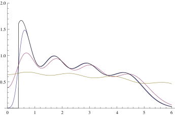
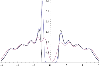
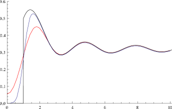
As an illustration we have plotted the densities in figure 1.

Figure 1: Example for the $\nu=0$ quenched density at finite $n=4$ at different masses: $m=0.4$ (top left plots) and $m=1$ (top right plots): the top black curves correspond to the shifted chGUE density eq. (4.29) at $a=0$ (which is clipped for $m=1$) ending at a sharp cutoff for $m>0$, see eq. (4.30). The density $\rho_{1}(x)$ eq. (LABEL:prelim) is plotted at various values of the deformation parameter $a$: at $a=0.1$ (top smooth blue curve), $a=0.3$ (middle smooth red curve), and at $a=0.9$ (lowest yellow curve) which is already indistinguishable from the GUE curve. Because the spectral density is symmetric due to $\nu=0$ we only show the positive eigenvalues. The lower plots show the same curves at $m=0$, the chGUE-GUE transition. Here $a=0$ and $a=0.1$ are already indistinguishable.

For comparison we also display the finite-$n$ density of the chGUE eq. (4.31) in the limit $a\to 0$. Switching on $a>0$ the smoothening of the hard wall provided by the Heaviside-Theta functions is nicely seen in figure 1.

Let us now spell out the density for $\nu=1$ explicitly and perform the limit $a\to 0$ there. In view of the relation between the polynomials eq. (4.17) it is useful to express the kernels for $\nu=1$ in terms of those with $\nu=0$ as well. We begin with the simplest kernel containing only polynomials and no integral transforms. After some algebra we obtain

$$D^{\nu=1}_{n}(x,y) = D_{n}(x,y)+\mbox{e}^{-\frac{(x^{2}+y^{2})}{4a^{2}}}\mbox{e}^{\frac{m^{2}}{2(1-a^{2})}}\frac{1}{8a\pi\sqrt{2\pi(1-a^{2})}}\left\{\int_{-\infty}^{\infty}ds\ \mbox{e}^{-s^{2}}L_{n}\left(\frac{(y+2ias)^{2}-m^{2}}{2(1-a^{2})}\right)\right.$$ (4.32)

$$\times\left.\int_{-\infty}^{\infty}dr\ \mbox{e}^{-r^{2}}(x+2iar+m)L^{(1)}_{n-1}\left(\frac{(x+2iar)^{2}-m^{2}}{2(1-a^{2})}\right)\ -\ (x\leftrightarrow y)\right\}\ ,$$

where we used the following identity for generalised Laguerre polynomials [35]

$$\sum_{j=0}^{n-1}L_{j}(z)=L^{(1)}_{n-1}(z)\ .$$ (4.33)

For the kernel determining the density we obtain after inserting the definitions

$$S^{\nu=1}_{n}(x,y) = \int_{-\infty}^{\infty}dzF(x-z)D^{\nu=1}_{n}(z,y)+\mbox{e}^{-\frac{y^{2}+2xm+m^{2}}{4a^{2}}}\frac{1}{2\pi a}\int_{-\infty}^{\infty}ds\ \mbox{e}^{-s^{2}}L_{n}\left(\frac{(y+2ias)^{2}-m^{2}}{2(1-a^{2})}\right).$$

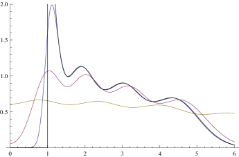
These two equations together with eq. (4) then determine the spectral density for $\nu=1$ shown in figure 2,

$$\rho_{1}^{\nu=1}(x)=S^{\nu=1}_{n}(x,x)\ .$$ (4.35)

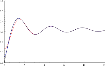
Figure 2: Example for the $\nu=1$ quenched density at finite $n=4$ at different masses: $m=0$ (left plots) and $m=1$ (right plots). Because for $m=0$ the density is still symmetric we only plot the positive eigenvalues. The black curves correspond to the (shifted) chGUE density at $a=0$. It can be nicely seen how the delta-function at $x=-m$ gets gradually smoothed out, where we show $a=0.1$ (blue curve) and $a=0.3$ (red curve).

We can now perform the limit $a\to 0$ as a check. The last term in eq. (LABEL:Snu1) gives a delta-function, $\delta(x+m)$, the exact zero-eigenvalue of the $\nu=1$ chGUE shifted to $x=-m$. Using the result eq. (4.29) and the above results for the limit at $\nu=0$ we obtain

$$\lim_{a\to 0}\rho^{\nu=1}_{1}(x) = |x|\,\mbox{e}^{-\frac{x^{2}}{2}+\frac{m^{2}}{2}}\sum_{j=0}^{n-1}L_{j}\left(\frac{x^{2}-m^{2}}{2}\right)^{2}\Theta(|x|-m)$$ (4.36)

$$-\ |x|\,\mbox{e}^{-\frac{x^{2}}{2}+\frac{m^{2}}{2}}L_{n}\left(\frac{x^{2}-m^{2}}{2}\right)L^{(1)}_{n-1}\left(\frac{x^{2}-m^{2}}{2}\right)\Theta(|x|-m)+\delta(x+m).$$

This can be seen as follows to be equivalent to the density of the chGUE at $\nu=1$

$$\rho_{1,\,\nu=1}^{chGU\!E}(y)=|y|^{3}\mbox{e}^{-y^{2}/2}\sum_{l=0}^{n-1}\frac{1}{2(l+1)}L_{l}^{(1)}(y^{2}/2)^{2}\ ,$$ (4.37)

shifted as in eq. (4.30). When using further identities [35]

$$XL_{l}^{(1)}(X)=(l+1)\Big{(}L_{l}(X)-L_{l+1}(X)\Big{)}\ ,\ \ L_{l}^{(1)}(X)=L_{l}(X)+L_{l-1}^{(1)}(X)\ ,$$ (4.38)

(and setting $L_{-1}\equiv 0$ here), we obtain the desired result, with $X\equiv\frac{1}{2}(x^{2}-m^{2})$,

$$X\sum_{l=0}^{n-1}\frac{1}{l+1}L_{l}^{(1)}(X)^{2} = \sum_{l=0}^{n-1}L_{l}^{(1)}(X)\Big{(}L_{l}(X)-L_{l+1}(X)\Big{)}$$ (4.39)

$$= \sum_{l=0}^{n-1}\Big{(}L_{l}(X)+L_{l-1}^{(1)}(X)\Big{)}L_{l}(X)\ -\sum_{l=0}^{n-1}L_{l}^{(1)}(X)L_{l+1}(X)$$

$$= \sum_{l=0}^{n-1}L_{l}(X)^{2}\ -\ L_{n-1}^{(1)}(X)L_{n}(X)\ .$$

5 The microscopic weakly non-chiral large-N limit

The microscopic large-$N$ limit is defined by the following rescaling of variables

$$\hat{x}\equiv\sqrt{2n}\,x\ ,\ \ \hat{a}\equiv\frac{1}{2}\sqrt{2n}\,a\ .$$ (5.1)

These variables are then to be identified with the variables in WchPT as given in eq. (2.9). Here we send the eigenvalues to zero and $n\to\infty$ such that $\hat{x}$ remains finite, hence we are in the vicinity of the origin. The masses $m$ and $z$ are rescaled likewise. Also the parameter $a$ corresponding to the effect of finite-lattice spacing in WchPT is sent to zero and $n\to\infty$ such that $\hat{a}$ remains finite. Thus we are in the vicinity of the chGUE ensemble which has chiral symmetry. For this reason we call this microscopic origin limit weakly non-chiral.

We begin with the asymptotic formulas of the partition function. Because we know the ($N_{f}=1$)-flavour partition function for finite-$N$ and general $\nu\geq 0$ we compute its asymptotic first. It reduces to the asymptotic for the even polynomials $R_{2j}$ at $\nu=0$. Based on the standard limit [35]

$$\lim_{n\rightarrow\infty}n^{-\nu}L_{n}^{(\nu)}\Big{(}\frac{x}{n}\Big{)}=x^{-\nu/2}J_{\nu}(2\sqrt{x})\ ,$$ (5.2)

we obtain the following expression:

$$\lim_{n,j\to\infty}\frac{(-)^{j}}{2^{j}j!}\langle\det[x+\hbox to0.0pt{ $\,\raisebox{0.6458pt}{/}\hss$}D_{5}]\rangle = \lim_{n\to\infty}(1-a^{2})^{j}\int_{-\infty}^{\infty}\frac{ds}{\sqrt{\pi}}\ \mbox{e}^{-s^{2}}(x+2ias-m)^{\nu}L_{j}^{(\nu)}\left(\frac{(x+2ias)^{2}-m^{2}}{2(1-a^{2})}\right)$$

$$= \mbox{e}^{-2t\hat{a}^{2}}\int_{-\infty}^{\infty}\frac{ds}{\sqrt{\pi}}\ \mbox{e}^{-s^{2}}t^{\frac{\nu}{2}}\left(\frac{\hat{m}-(\hat{x}+4is\hat{a})}{\hat{m}+\hat{x}+4is\hat{a}}\right)^{\frac{\nu}{2}}I_{\nu}\Big{(}\sqrt{t(\hat{m}^{2}-(\hat{x}+4is\hat{a})^{2})}\Big{)}.$$

First we have divided out part of the normalisation that cancels with the norms $r_{j}$ in the sums inside the kernels. Second we have given the result for $j=tn$ with $t\in[0,1]$ as we will need these later when replacing the sum inside the kernel by an integral. Last we have used that due to the rescaling the prefactor turns into an exponential,

$$(1-ja^{2}/j)^{j}\to\exp[-ja^{2}]=\exp[{-2t\hat{a}^{2}}]\ .$$ (5.4)

The result eq. (LABEL:vevlim) matches that of the partition function eq. (A.10) as it should.

The limiting even polynomial $R_{2j}(x)$ for $\nu=0$ is obtained by simply setting $\nu=0$ everywhere in eq. (LABEL:vevlim) (due to parity there is no need to switch $x\to-x$ under the determinant):

$$\lim_{n,j\to\infty}\frac{(-)^{j}}{2^{j}j!}R_{2j}(x) = \mbox{e}^{-2t\hat{a}^{2}}\int_{-\infty}^{\infty}\frac{ds}{\sqrt{\pi}}\mbox{e}^{-s^{2}}I_{0}\Big{(}\sqrt{t(\hat{m}^{2}-(\hat{x}+4is\hat{a})^{2})}\Big{)}\ .$$

The computation of the limiting odd polynomials $R_{2j+1}(x)$ for $\nu=0$ is now a simple consequence. Starting from the explicit form eq. (4.6) we obtain

$$\lim_{n,j\to\infty}\sqrt{2n}\frac{(-)^{j}}{2^{j}j!}R_{2j+1}(x) = \mbox{e}^{-2t\hat{a}^{2}}\int_{-\infty}^{\infty}\frac{ds}{\sqrt{\pi}}\ e^{-s^{2}}(\hat{x}+4is\hat{a})I_{0}\Big{(}\sqrt{t(\hat{m}^{2}-(\hat{x}+4is\hat{a})^{2})}\Big{)}\ ,$$ (5.6)

after an integration by parts. As a check the asymptotic of the odd polynomial is an odd function in $\hat{x}$. Note that both prefactors from eq. (5.4) will cancel with the limiting norms $r_{j}$.

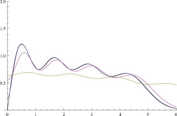
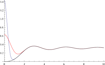
Figure 3: The microscopic density eq. (LABEL:rhomicro) for $\hat{m}=1$ (top left plots) and $\hat{m}=3$ (top right plots) at various values of $\hat{a}=0.1$ (middle blue curves) and $\hat{a}=0.25$ (lower red curves). For comparison we also show the corresponding chGUE density ($\hat{a}=0$) eq. (5.11) shifted as in eq. (4.30) (top black curves). For the chGUE-GUE transition at $\hat{m}=0$ (bottom plots) the difference to $\hat{a}=0.1$ or $\hat{a}=0.25$ is almost indistinguishable, apart from the origin.

For the limiting weight $F(x)$ from eq. (3) we get a Gaussian times the error-functions:

$$\lim_{n\to\infty}F(x)=\exp\Big{[}\frac{\hat{x}^{2}}{32\hat{a}^{2}}\Big{]}\left[\mbox{erf}\left(\frac{\hat{x}}{4\sqrt{2\hat{a}^{2}}}+\frac{\hat{m}}{2\sqrt{2\hat{a}^{2}}}\right)+\mbox{erf}\left(\frac{\hat{x}}{4\sqrt{2\hat{a}^{2}}}-\frac{\hat{m}}{2\sqrt{2\hat{a}^{2}}}\right)\right].$$ (5.7)

Collecting all results we obtain the quenched $\nu=0$ microscopic density $\rho_{S}(\hat{x})\equiv\lim_{n\to\infty}\frac{1}{\sqrt{2n}}\rho_{1}(x)$:

$$\rho_{S}(\hat{x}) = \int_{-\infty}^{\infty}d\hat{y}\frac{\mbox{e}^{-\frac{(\hat{x}+\hat{y})^{2}}{32\hat{a}^{2}}}}{32\sqrt{2\hat{a}^{2}\pi}}\left(\mbox{erf}\Big{(}\frac{\hat{y}-\hat{x}+2\hat{m}}{4\sqrt{2\hat{a}^{2}}}\Big{)}+\mbox{erf}\Big{(}\frac{\hat{y}-\hat{x}-2\hat{m}}{4\sqrt{2\hat{a}^{2}}}\Big{)}\right)\int_{-\infty}^{\infty}\frac{ds\,dr}{{\pi}}\mbox{e}^{-s^{2}-r^{2}}$$

$$\times\int_{0}^{1}dt(\hat{x}-\hat{y}+4i\hat{a}(r-s))I_{0}\Big{(}\sqrt{t(\hat{m}^{2}-(\hat{y}+4is\hat{a})^{2})}\Big{)}I_{0}\Big{(}\sqrt{t(\hat{m}^{2}-(\hat{x}+4ir\hat{a})^{2})}\Big{)}$$

$$= \int_{-\infty}^{\infty}d\hat{y}\frac{\mbox{e}^{-\frac{(\hat{x}+\hat{y})^{2}}{32\hat{a}^{2}}}}{16\sqrt{2\hat{a}^{2}\pi}}\left(\mbox{erf}\Big{(}\frac{\hat{y}-\hat{x}+2\hat{m}}{4\sqrt{2\hat{a}^{2}}}\Big{)}+\mbox{erf}\Big{(}\frac{\hat{y}-\hat{x}-2\hat{m}}{4\sqrt{2\hat{a}^{2}}}\Big{)}\right)\int_{-\infty}^{\infty}\frac{ds\,dr}{{\pi}}\mbox{e}^{-s^{2}-r^{2}}$$

$$\times\frac{\sqrt{\hat{m}^{2}-(\hat{x}+4ir\hat{a})^{2}}I_{0}\Big{(}\sqrt{\hat{m}^{2}-(\hat{y}+4is\hat{a})^{2}}\Big{)}I_{1}\Big{(}\sqrt{\hat{m}^{2}-(\hat{x}+4ir\hat{a})^{2}}\Big{)}-(\hat{x}\leftrightarrow\hat{y})}{\hat{x}+\hat{y}+4i\hat{a}(s+r)}\ .$$

It is shown in figure 3. Here we give both forms, before and after using the Christoffel-Darboux identity which has its large-$N$ correspondence in

$$\int_{0}^{1}dtI_{0}(X\sqrt{t})I_{0}(Y\sqrt{t})=\frac{2XI_{0}(Y)I_{1}(X)-2YI_{0}(X)I_{1}(Y)}{X^{2}-Y^{2}}\ .$$ (5.9)

Unfortunately we have been unable to check analytically that eq. (LABEL:rhomicro) is equivalent to the corresponding density given in [20]. There it is given as the discontinuity of the imaginary part of its resolvent.

As a check we can again take the limit $\hat{a}\to 0$, and we obtain from the first form in eq. (LABEL:rhomicro)

$$\lim_{\hat{a}\to 0}\rho_{S}(\hat{x}) = \frac{|\hat{x}|}{2}\Theta(|\hat{x}|-\hat{m})\int_{0}^{1}dtJ_{0}\left(\sqrt{t(\hat{x}^{2}-\hat{m}^{2})}\right)^{2}$$ (5.10)

$$= \frac{|\hat{x}|}{2}\Theta(|\hat{x}|-\hat{m})\Big{[}J_{0}\left(\sqrt{\hat{x}^{2}-\hat{m}^{2}}\right)^{2}+J_{1}\left(\sqrt{\hat{x}^{2}-\hat{m}^{2}}\right)^{2}\Big{]}.$$

It equals the shifted microscopic density of the chGUE at $\nu=0$ after the shift in eq. (4.30)

$$\rho_{S}^{chGU\!E}(\hat{x})=\frac{|\hat{x}|}{2}\Big{(}J_{0}(\hat{x})^{2}+J_{1}(\hat{x})^{2}\Big{)}\ .$$ (5.11)

We now turn to the limiting density for $\nu=1$. Starting from eqs. (4.32) and (LABEL:Snu1) it is useful to write it as the limiting density at $\nu=0$ which we have already determined, plus a correction term. Collecting all terms and using the asymptotic expressions from above we arrive at

$$\rho_{S}^{\nu=1}(\hat{x}) = \rho_{S}(\hat{x})\ +\ \int_{-\infty}^{\infty}d\hat{z}\frac{\mbox{e}^{-\frac{(\hat{x}+\hat{z})^{2}}{32\hat{a}^{2}}}}{16\hat{a}\pi\sqrt{2\pi}}\left(\mbox{erf}\Big{(}\frac{\hat{x}-\hat{z}+2\hat{m}}{4\sqrt{2\hat{a}^{2}}}\Big{)}+\mbox{erf}\Big{(}\frac{\hat{x}-\hat{z}-2\hat{m}}{4\sqrt{2\hat{a}^{2}}}\Big{)}\right)$$ (5.12)

$$\times\left\{\int_{-\infty}^{\infty}ds\,\mbox{e}^{-s^{2}}I_{0}\Big{(}\sqrt{\hat{m}^{2}-(\hat{x}+4is\hat{a})^{2}}\Big{)}\int_{-\infty}^{\infty}dr\,\mbox{e}^{-r^{2}}{\frac{\hat{m}+\hat{z}+4i\hat{a}r}{\sqrt{\hat{m}^{2}-(\hat{z}+4i\hat{a}r)^{2}}}}\right.$$

$$\ \ \ \ \ \ \ \ \times\left.I_{1}\Big{(}\sqrt{\hat{m}^{2}-(\hat{z}+4ir\hat{a})^{2}}\Big{)}\ -\ (\hat{x}\leftrightarrow\hat{z})\right\}$$

$$+\ \frac{1}{4\pi\hat{a}}\mbox{e}^{-\frac{(\hat{x}+\hat{m})^{2}}{16\hat{a}^{2}}}\int_{-\infty}^{\infty}ds\,\mbox{e}^{-s^{2}}I_{0}\Big{(}\sqrt{\hat{m}^{2}-(\hat{x}+4is\hat{a})^{2}}\Big{)},$$

which we illustrate in figure 4.

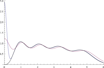
Figure 4: The microscopic density eq. (5.12) for $\hat{m}=0$ (left plots) and $\hat{m}=3$ (right plots) at various values of $\hat{a}=0.3$ (red curves), $\hat{a}=0.1$ (blue curves), and $\hat{a}=0$ (black curves) for comparison. For the chGUE-GUE transition at $\hat{m}=0$ the density is still symmetric and we only display $\hat{x}>0$. For $\hat{m}>0$ the delta-function is shifted to the left, and we can nicely see its increasing broadening from $\hat{a}=0.1$ to $\hat{a}=0.25$.

Once more we can perform as a check the limit $\hat{a}\to 0$, and we obtain

$$\lim_{\hat{a}\to 0}\rho_{S}^{\nu=1}(\hat{x}) = \lim_{\hat{a}\to 0}\rho_{S}(\hat{x})-\frac{|\hat{x}|}{\sqrt{\hat{x}^{2}-\hat{m}^{2}}}J_{0}\left(\sqrt{\hat{x}^{2}-\hat{m}^{2}}\right)J_{1}\left(\sqrt{\hat{x}^{2}-\hat{m}^{2}}\right)\Theta(|\hat{x}|-\hat{m})\ +\ \delta(\hat{x}+\hat{m})\ .$$

The matching with the density of the chGUE at $\nu=1$,

$$\rho_{S,\,\nu=1}^{chGU\!E}(\hat{x})=\frac{|\hat{x}|}{2}\Big{(}J_{1}(\hat{x})^{2}-J_{0}(\hat{x})J_{2}(\hat{x})\Big{)}\ ,$$ (5.14)

shifted as in eq. (4.30) can be seen as follows:

$$\rho_{S,\,\nu=1}^{chGU\!E}(X)-\rho_{S}^{chGU\!E}(X) = -\frac{X}{2}J_{0}(X)(J_{2}(X)+J_{0}(X))$$ (5.15)

$$= -J_{0}(X)J_{1}(X)\ .$$

Here we used a Bessel identity and the abbreviation $X=\sqrt{\hat{x}^{2}-\hat{m}^{2}}$. The delta-function in eq. (LABEL:rhonu1lim) is just the exact zero-eigenvalue at $\hat{x}=-\hat{m}$, originating from the last term in eq. (5.12) which is non-Gaussian.

6 Conclusions

In this paper we have introduced a parameter dependent Gaussian random two-matrix model that interpolates between the chGUE ($a=0$) and the GUE ($a=1$) symmetry class (possibly shifted by a constant matrix). At the same time this model describes the spectral properties of the Hermitian Wilson Dirac operator when we take the microscopic weakly non-chiral limit at the origin. Here the rescaled parameter $\hat{a}\sim a\sqrt{n}$ is interpreted as the effect of finite lattice spacing. It is properly incorporated in a continuum effective field theory as Wilson chiral Perturbation theory in the epsilon regime to order ${\cal O}(\hat{a}^{2})$.

We have completely determined all spectral $k$-point density correlation functions when starting from a chGUE of size $(2n+\nu)$ with $\nu=0$ or $\nu=1$ exact zero modes, both for finite $n$ and in the microscopic large-$n$ origin limit at weak non-chirality. They are given in terms of the Pfaffian of a $2\times 2$ matrix kernel, containing three individual kernels as building blocks. Each kernel is expressed as a sum over skew-orthogonal polynomials (and their integral transforms) depending on $\nu=0$ or 1, which we explicitly constructed in terms of Gaussian integrals over Laguerre polynomials. In the large-$n$ limit these 3 respective kernels contain in their final form a fixed number of 2 up to 4 Gaussian integrals over modified Bessel functions, respectively. The Pfaffian of the matrix kernel is thus easily evaluated for any $k$-point function.

Let us compare to what is known in the literature. In [20, 21] the supersymmetric method was used to compute the microscopic spectral density ($k=1$) directly from the chiral Lagrangian for arbitrary $\nu$, the so-called index. In [26] this was extended to include one ($N_{f}=1$) extra quark determinant. This method rapidly becomes cumbersome when adding more flavours $N_{f}>1$ or increasing $k$, as the number of integrations increases with the dimension of the auxiliary supermatrix from the Hubbard-Stratonovich transformation. This problem was partly circumvented in [27] by using the graded supereigenvalue method, where explicit examples where provided for the density $k=1$ up to $N_{f}=2$, and for the two-point density $k=2$ quenched. However, also here it is difficult to establish the Pfaffian structure of the $k$-point functions, and thus the number of integrals grows with $k$ and $N_{f}$ for the $k$-point density correlation function (for recent progress see however [36]).

It is an open problem how to include both $N_{f}>0$ and $\nu>1$ in our skew-orthogonal polynomial method, in particular the latter, as the joint probability distribution of eigenvalues which we computed here for the general $N_{f}$ and $\nu$ case is no longer a simple Pfaffian of a single block matrix for $\nu>0$. The reason for attempting this problem in the future is not only an independent confirmation for the aforementioned analytical results which are mainly for $k=1$. The extension to arbitrary $k$ is crucial if we want to get a hand on individual eigenvalue distributions at least in a perturbative expansion (see e.g. [9]), apart from the conceptual aspect of integrability of our two-matrix model. Furthermore, in all works [20, 21, 26, 27] also the density of real eigenvalues of the complex non-Hermitian Wilson Dirac operator was considered. The extension to this operator is another challenge to our method.

Acknowledgments: It is a pleasure to thank P. Damgaard, M. Kieburg, K. Splittorff, and J. Verbaarschot for collaborations on related topics and many discussions. The Niels Bohr Institute and Niels Bohr International Academy are thanked (G.A.) for hospitality and partial financial support when this work was initiated. This work was partially supported by the Japan Society for the Promotion of Science (KAKENHI 20540372) (T.N.).

Appendix A Equivalence to the partition function of WchPT

In this appendix we show the equivalence of our matrix model in the microscopic limit to WchPT in the epsilon regime, as it was displayed in eq. (2.7). For non-degenerate parameters we have

$${\cal Z}_{\nu}^{(N_{f})} \sim \int dAdBdWd\Omega\prod_{f=1}^{N_{f}}\det\left[\begin{array}[]{cc}(z_{f}+m_{f})\leavevmode\hbox{\small 1\kern-3.8pt\normalsize 1}_{n}+A&W+\Omega\\ W^{\dagger}+\Omega^{\dagger}&(z_{f}-m_{f})\leavevmode\hbox{\small 1\kern-3.8pt\normalsize 1}_{n+\nu}+B\\ \end{array}\right]\mbox{e}^{-\frac{1}{2(1-a^{2})}{\mbox{Tr}}(WW^{\dagger})}$$ (A.4)

$$\times\mbox{e}^{-\frac{1}{4a^{2}}{\mbox{Tr}}(A^{2}+B^{2}+2\Omega\Omega^{\dagger})}\ .$$

Defining $z_{f}^{\pm}\equiv z_{f}\pm m_{f}$ we now express the determinants as integrals over $N_{f}$ sets of complex Grassmann variables $\eta_{i}^{f}$, $i=1,\ldots,n$ and $\psi_{b}^{f}$, $b=1,\ldots,n+\nu$,

$$\prod_{f=1}^{N_{f}}\det[\ldots] = \int d^{2}\eta d^{2}\psi\mbox{e}^{\eta_{i}^{*\,f}(z^{+}_{f}\delta_{ij}+A_{ij})\eta_{j}^{f}+\psi^{*\,f}_{b}(W_{bj}^{\dagger}+\Omega_{bj}^{\dagger})\eta_{i}^{f}+\eta_{i}^{*\,f}(W_{ib}+\Omega_{ib})\psi_{b}^{f}+\psi^{*\,f}_{c}(z_{f}^{-}\delta_{cb}+B_{cb})\psi_{b}^{f}}\ ,\ \ \ \$$ (A.5)

using summation conventions in all indices. A completion of the squares and integration of the Gaussian matrices yields

$${\cal Z}_{\nu}^{(N_{f})} \sim \int d^{2}\eta d^{2}\psi\ e^{z^{+}_{f}\eta^{*\,f}_{i}\eta_{i}^{f}+z^{-}_{f}\psi^{*\,f}_{b}\psi_{b}^{f}-a^{2}\left((\eta^{*\,f}_{i}\eta_{i}^{f})^{2}+(\psi^{*\,f}_{b}\psi_{b}^{f})^{2}\right)-2\psi^{*\,f}_{b}\psi_{b}^{f}\eta^{*\,g}_{i}\eta_{i}^{g}}$$

$$= \int dQ_{1}dQ_{2}dT\det[Z^{+}-i\sqrt{2}(aQ_{1}+T^{\dagger})]^{n}\det[Z^{-}-i\sqrt{2}(aQ_{2}+T)]^{n+\nu}\mbox{e}^{-{\mbox{Tr}}(TT^{\dagger}+Q_{1}^{2}+Q_{2}^{2})}\ .$$

Here we have introduced two Hermitian matrices $Q_{1,2}$ and one complex non-Hermitian matrix $T$ of size $N_{f}\times N_{f}$ to do the Hubbard-Stratonovich transformation. Integrating out all Grassmann variables yields an exact expression containing the diagonal matrices $Z^{\pm}$ with elements $z_{f}^{\pm}$ (up to some constant prefactors that we dropped). If we parametrise $T=UR$ with $U$ unitary and $R$ positive definite Hermitian the saddle point is taken at $R\sim\leavevmode\hbox{\small 1\kern-3.8pt\normalsize 1}_{N_{f}}\sqrt{n}$ when we employ the scaling of masses and $a$ indicated in eq. (2.9). We obtain

$$\lim_{n\to\infty}{\cal Z}_{\nu}^{(N_{f})} \sim \int dQ_{1}dQ_{2}\int dU\det[U]^{\nu}\mbox{e}^{\frac{i}{2}{\mbox{Tr}}(\hat{Z}^{+}U+\hat{Z}^{-}U^{\dagger})+\sqrt{2\hat{a}^{2}}{\mbox{Tr}}(Q_{1}U+Q_{2}U^{\dagger})-\frac{1}{2}{\mbox{Tr}}(Q_{1}^{2}+Q_{2}^{2})}$$ (A.7)

$$\sim \int dU\det[U]^{\nu}\exp\Big{[}\frac{1}{2}{\mbox{Tr}}(\hat{M}(U+U^{\dagger}))+\frac{1}{2}{\mbox{Tr}}(\hat{Z}(U-U^{\dagger}))-\hat{a}^{2}{\mbox{Tr}}(U^{2}+U^{{\dagger}\,2})\Big{]}\ ,\ \ \ \$$

after integrating out the matrices $Q_{1,2}$ and performing a further rotation $U\to iU$, $U^{\dagger}\to-iU^{\dagger}$. Eq. (A.7) is the partition function of WchPT in the epsilon regime for non-degenerate masses, hence we have completed our claimed proof.

A.1 Alternative representation of $N_{f}=1$ WchPT

Finally we would like to make the equivalence between the $N_{f}=1$ flavour partition function for the large-$N$ limit of our even polynomials $R_{2n}(x)$ explicit. The reason why we present this check in detail is that we require a slightly different form from the one given in [20] eq. (13), or in [21] eq. (151) (for $\hat{z}=0$ there):

$${Z}_{\nu}^{(N_{f}=1)}(\hat{m},\hat{z},\hat{a}) = \mbox{e}^{-2\hat{a}^{2}}\int_{-\pi}^{\pi}\frac{d\theta}{2\pi}\mbox{e}^{i\theta\nu}\exp[\hat{m}\cos(\theta)+i\hat{z}\sin(\theta)+4\hat{a}^{2}\sin^{2}(\theta)]$$ (A.8)

$$= \mbox{e}^{-2\hat{a}^{2}}\int_{-\pi}^{\pi}\frac{d\theta}{2\pi}\mbox{e}^{i\theta\nu}\int_{-\infty}^{\infty}\frac{dx}{\sqrt{\pi}}\mbox{e}^{-x^{2}}\exp[\hat{m}\cos(\theta)+i\hat{z}\sin(\theta)-4x\hat{a}\sin(\theta)]\ ,\ \ \ \$$

where after using a trigonometric identity we have linearised the sine-squared term instead. We can now use the following identity [37] for generic matrices $A,B$

$$\int_{U(N_{f})}\det[U]^{\nu}\exp\left[\frac{1}{2}{\mbox{Tr}}(AU+BU^{\dagger})\right]\ =\ 2^{N_{f}(N_{f}-1)/2}\prod_{j=1}^{N_{f}-1}j!\ \left(\frac{\det[B]}{\det[A]}\right)^{\nu/2}\frac{\det[\mu_{i}^{j-1}I_{\nu+j-1}(\mu_{i})]}{\Delta_{N_{f}}(\{\mu^{2}\})}\ ,$$ (A.9)

with $\mu_{i}^{2}$ being the eigenvalues of the product matrix $AB$. Specifying to $U=e^{i\theta}\in U(1)$ and identifying $A=\hat{m}+\hat{z}+4ix\hat{a}$, $B=\hat{m}-(\hat{z}+4ix\hat{a})$ we arrive at

$${Z}_{\nu}^{(N_{f}=1)}(\hat{m},\hat{z},\hat{a})=\mbox{e}^{-2\hat{a}^{2}}\int_{-\infty}^{\infty}\frac{dx}{\sqrt{\pi}}\mbox{e}^{-x^{2}}\left(\frac{\hat{m}-(\hat{z}+4ix\hat{a})}{\hat{m}+\hat{z}+4ix\hat{a}}\right)^{\nu/2}I_{\nu}\Big{(}\sqrt{\hat{m}^{2}-(\hat{z}+4ix\hat{a})^{2}}\Big{)}\ ,$$ (A.10)

which agrees perfectly with eq. (LABEL:vevlim), see also eq. (99) in [27].

Appendix B Consistency checks of the partition function and factorisation

In this appendix we perform a few consistency checks of the eigenvalue representation of the partition function eq. (3.50). For simplicity we will set $m=0$ and $N_{f}=0$ here. The antisymmetric weight eq. (3) thus reduces to

$$F(x)|_{m=0}=2\ \mbox{e}^{\frac{x^{2}(1-a^{2})}{8a^{2}}}\mbox{erf}\Big{(}\frac{x\sqrt{1-a^{2}}}{2\sqrt{2a^{2}}}\Big{)}\ .$$ (B.1)

B.1 The GUE limit $a\to 1$ for $\nu=0$

On the level of the distribution eq. (2.2) it is clear that the matrix $W$ gets suppressed for $a\to 1$. After reducing to eigenvalues the same result should come out. Here we will look at the simplest case only, that is $\nu=0$. We can insert the simplification eq. (B.1) into eq. (3.52) at $\nu=0$. Noting that in the limit $a\to 1$ the exponential factor in eq. (B.1) reduces to unity, we can use the following result of [28] (see end of section 3 in the first paper) for the limit of a Pfaffian of an error-function,

$$\lim_{a\to 1}\mbox{Pf}_{1\leq i,j\leq 2n}\left[\mbox{erf}\left((d_{i}-d_{j})\sqrt{\frac{(1-a^{2})}{8a^{2}}}\right)\right]\sim\ \Delta_{2n}(\{d\})\ .$$ (B.2)

This provides the second Vandermonde determinant in eq. (3.52) to constitute the GUE, and we arrive at

$$\lim_{a\to 1}{\cal Z}_{\nu=0}^{(N_{f}=0)}|_{m=0}\sim\int_{-\infty}^{\infty}\prod_{j=1}^{N}dd_{j}\,d_{j}^{N_{f}}\exp\Big{[}{-\frac{d_{j}^{2}}{4}}\Big{]}\ \Delta_{N}(\{d\})^{2}\ .$$ (B.3)

B.2 The chGUE limit $a\to 0$ and factorisation

Here we would like to perform a more detailed check. As it was shown in [21] in the large-$N$ limit the spectral density of the Hermitian Wilson Dirac operator behaves like the density of a finite GUE-matrix of size $\nu\times\nu$ plus the microscopic chGUE density. We therefore expect that our general partition function will factorise in the limit $a\to 0$ into a finite GUE times a second chGUE partition function of the remaining $2n$ eigenvalues.

In order to show that we will first simplify ${\cal Z}_{\nu}^{(0)}$ further before using the de Bruijn integration theorem. Taking eq. (LABEL:Zev) as a starting point we can use the fact that the jpdf integrated over all variables is totally symmetric under exchange or relabeling of the $d_{j}$ . We can split the variables into two sets, denoted by $t_{j=1,\ldots,\nu}\equiv d_{j=1,\ldots,\nu}$, and $s_{j=1,\ldots,2n}\equiv d_{j=\nu+1,\ldots,2n+\nu}$. If we do a Laplace expansion of the determinant into blocks of sizes $2n\times 2n$ and $\nu\times\nu$, we can split off a Vandermonde type determinant in the variables $t_{j}$, after appropriately relabeling all other permutations:

$${\cal Z}_{\nu}^{(0)} \sim \int_{-\infty}^{\infty}\prod_{j=1}^{\nu}dt_{j}\,\mbox{e}^{-\frac{t_{j}^{2}}{4a^{2}}}\Delta_{\nu}(\{t\})\int_{-\infty}^{\infty}\prod_{j=1}^{2n}ds_{j}\,\mbox{e}^{-\frac{s_{j}^{2}}{4a^{2}}}\prod_{i=1}^{\nu}(s_{j}-t_{i})\ \Delta_{2n}(\{s\})$$ (B.11)

$$\times\int_{0}^{\infty}\prod_{b=1}^{n}du_{b}\mbox{e}^{\frac{-u_{b}^{2}}{2a^{2}(1-a^{2})}}\left|\begin{array}[]{cc}\mbox{e}^{\frac{s_{1}u_{1}}{2a^{2}}}\ldots\mbox{e}^{\frac{s_{1}u_{n}}{2a^{2}}}&\mbox{e}^{-\frac{s_{1}u_{1}}{2a^{2}}}\ldots\mbox{e}^{-\frac{s_{1}u_{n}}{2a^{2}}}\\ \cdots&\cdots\\ \mbox{e}^{\frac{s_{2n}u_{1}}{2a^{2}}}\ldots\mbox{e}^{\frac{s_{2n}u_{n}}{2a^{2}}}&\mbox{e}^{-\frac{s_{2n}u_{1}}{2a^{2}}}\ldots\mbox{e}^{-\frac{s_{2n}u_{n}}{2a^{2}}}\\ \end{array}\right|\left|\begin{array}[]{cccc}1&{t_{1}}&\cdots&t_{1}^{\nu-1}\\ \cdots&\cdots&\cdots&\cdots\\ 1&t_{\nu}&\cdots&t_{\nu}^{\nu-1}\end{array}\right|\!\!.$$

We can now perform the integrations over $u_{1},\ldots,u_{n}$ with the help of the standard de Bruijn integral formula eq. (LABEL:gendeB). To make it applicable we can simply multiply the weight factors into the determinant, and we obtain the following result:

$${\cal Z}_{\nu}^{(0)}\! \sim \!\int_{-\infty}^{\infty}\prod_{j=1}^{\nu}dt_{j}\,\mbox{e}^{-\frac{t_{j}^{2}}{4a^{2}}}\Delta_{\nu}(\{t\})^{2}\!\int_{-\infty}^{\infty}\prod_{j=1}^{2n}ds_{j}\,\mbox{e}^{-\frac{s_{j}^{2}}{4a^{2}}}\prod_{i=1}^{\nu}(s_{j}-t_{i})\Delta_{2n}(\{s\})\mbox{Pf}_{1\leq i,j\leq 2n}\left[F(s_{i}-s_{j})\right]\!.\ \ \ \ \ \ \$$ (B.12)

In eq. (B.12) we can make further use of the symmetry under relabeling of the variables $s_{j}$ and the anti-symmetry of the Vandermonde determinant to write the Pfaffian as the following product:

$${\cal Z}_{\nu}^{(0)} \sim \int_{-\infty}^{\infty}\prod_{j=1}^{\nu}dt_{j}\,\mbox{e}^{-\frac{t_{j}^{2}}{4a^{2}}}\Delta_{\nu}(\{t\})^{2}\!\int_{-\infty}^{\infty}\prod_{j=1}^{2n}ds_{j}\,\mbox{e}^{-\frac{s_{j}^{2}}{4a^{2}}}\prod_{i=1}^{\nu}(s_{j}-t_{i})\ \Delta_{2n}(\{s\})\prod_{k=1}^{n}F(s_{2k}-s_{2k-1}).\ \ \ \ \ \$$ (B.13)

Now consider the exponents of two consecutive variables, say $s_{1}$ and $s_{2}$, from the Gaussian and the exponential part of $F$:

$$\exp\Big{[}{-\frac{s_{1}^{2}+s_{2}^{2}}{4a^{2}}}+\frac{(s_{2}-s_{1})^{2}(1-a^{2})}{8a^{2}}\Big{]}=\exp\Big{[}-\frac{(s_{1}+s_{2})^{2}}{8a^{2}}-\frac{(s_{1}-s_{2})^{2}}{8}\Big{]}.$$ (B.14)

In the limit $a\to 0$ the first term on the right hand side will give a delta-function, whereas the second Gaussian term remains:

$$\lim_{a\to 0}\sqrt{8a^{2}\pi}\exp\Big{[}-\frac{(s_{1}+s_{2})^{2}}{8a^{2}}-\frac{(s_{1}-s_{2})^{2}}{8}\Big{]}=\delta(s_{1}+s_{2})\ \mbox{e}^{-s_{1}^{2}/2}\ .$$ (B.15)

In the same limit the error-function in eq. (B.1) becomes the sign function (see e.g. [28]),

$$\lim_{a\to 0}\mbox{erf}\Big{[}(s_{2}-s_{1})\sqrt{\frac{(1-a^{2})}{8a^{2}}}\Big{]}=\mbox{sign}[s_{2}-s_{1}]\ .$$ (B.16)

We are now ready to take the limit $a\to 0$ of the partition function eq. (B.13). We first formally change variables $r_{j}=t_{j}/a$ to isolate the $a$-dependence, and then take the limit only on the remaining $a$-dependence, that is the variables $r_{j}$,

$$\lim_{a\to 0}{\cal Z}_{\nu}^{(0)}\sim\int_{-\infty}^{\infty}\prod_{j=1}^{\nu}dr_{j}\,\mbox{e}^{-\frac{r_{j}^{2}}{4}}\Delta_{\nu}(\{r\})^{2}\int_{-\infty}^{\infty}\prod_{j=1}^{n}ds_{j}\,s_{j}\mbox{sign}[s_{j}]\exp\Big{[}{-\frac{s_{j}^{2}}{2}}\Big{]}\prod_{i=1}^{\nu}(s_{j}^{2}-a^{2}r_{i}^{2})\ \Delta_{n}(\{s^{2}\})^{2}.$$ (B.17)

We have used the fact that for $s_{2k}\to-s_{2k-1}$ we obtain $\Delta_{2n}(\{s\})\to\prod_{i=1}^{n}2s_{i}\ \Delta_{n}(\{s^{2}\})^{2}$. The variables $r_{j}$ thus act as mass terms to the $s$-variables, but to leading order these masses can be neglected, leading to a complete decoupling of variables. Our final result is thus reading

$$\int_{-\infty}^{\infty}\prod_{j=1}^{\nu}dr_{j}\,\exp\Big{[}{-\frac{r_{j}^{2}}{4}}\Big{]}\Delta_{\nu}(\{r\})^{2}\int_{-\infty}^{\infty}\prod_{j=1}^{n}ds_{j}\,|s_{j}|^{2\nu+1}\exp\Big{[}{-\frac{s_{j}^{2}}{2}}\Big{]}\ \Delta_{n}(\{s^{2}\})^{2},$$ (B.18)

where the $\nu$ would-be zero-eigenvalues at $a=0$ have decoupled into a GUE of size $\nu$, times the standard massless chGUE with exactly $\nu$ zero eigenvalues. However, we should remember that due to rescaling the original variables $t_{j}$ are all of the order ${\cal O}(a)$.

It is clear how to this order of approximation the microscopic spectral density would look like: it is the superposition of a finite-$\nu$ semi-circle from the GUE and the Bessel spectral density with $\nu$ zero-eigenvalues from the chGUE. This confirms the analysis of [21] on the level of the partition function, to that order.

Appendix C Skew-orthogonal polynomials

In this appendix we compute the skew-orthogonal polynomials given in eqs. (4.6) for $\nu=0$. We first recall that the expectation value of a single characteristic polynomial (or equivalently the $N_{f}=1$ partition function) gives the even polynomials $R_{2j}$ where we follow the argument of [38]. This expectation value is computed using the supersymmetric method in the next subsection C.1. Based on that the odd polynomials $R_{2j+1}$ then follow as shown in C.2.

Starting from the quenched partition function eq. (3.52) for $\nu=0$

$${\cal Z}_{0}^{(0)}=\int_{-\infty}^{\infty}\prod_{j=1}^{2n}ds_{j}w(s_{j})\ \Delta_{2n}(\{s\})\ \mbox{Pf}_{1\leq i,j\leq 2n}[F(s_{i}-s_{j})]\ ,$$ (C.1)

we can write the expectation value of a single determinant as follows:

$$\langle\det[z-\hbox to0.0pt{ $\,\raisebox{0.6458pt}{/}\hss$}D_{5}]\rangle_{2n} = \frac{1}{{\cal Z}_{0}^{(0)}}\int_{-\infty}^{\infty}\prod_{j=1}^{2n}ds_{j}w(s_{j})(z-s_{j})\ \Delta_{2n}(\{s\})\ \mbox{Pf}_{1\leq i,j\leq 2n}[F(s_{i}-s_{j})]$$ (C.2)

$$= \frac{1}{{\cal Z}_{0}^{(0)}}\frac{(2n)!}{2^{n}n!}\int_{-\infty}^{\infty}\prod_{j=1}^{N}ds_{j}w(s_{j})\ \Delta_{2n+1}(\{s\},z)\ \prod_{l=1}^{n}F(s_{2l}-s_{2l-1}).$$

Here we have used the fact that both the Vandermonde determinant and the Pfaffian are antisymmetric in order to simplify their product (times the symmetric integral over all eigenvalues), cf. [29] Appendix 25. Furthermore we have included the determinant into a larger Vandermonde. Writing the Vandermonde determinant in terms of even and odd monic polynomials $\Phi_{2i}$ and $\Psi_{2i+1}$ respectively,

$$\Delta_{2n+1}(\{s\},z)=\det_{i=0,\ldots,n-1;j=1,\ldots,2n+1}\Big{[}\{\Phi_{2i}(s_{j}),\Psi_{2i+1}(s_{j})\}\ \Phi_{2n}(s_{j})\Big{]}\ ,$$ (C.3)

and relabeling $z=s_{2n+1}$, we have from the generalised de Bruijn formula (cf. [38] eq. (4.9), or [34])

$$\langle\det[z-\hbox to0.0pt{ $\,\raisebox{0.6458pt}{/}\hss$}D_{5}]\rangle_{2n}=\frac{n!}{{\cal Z}_{0}^{(0)}}\ \mbox{Pf}_{0\leq i,j\leq 2n}\left[\begin{array}[]{lll}\langle\varphi_{i},\varphi_{j}\rangle&\ldots&\varphi_{0}(s_{2n+1})\\ \ldots&&\cdots\\ &&\varphi_{2n}(s_{2n+1})\\ -\varphi_{0}(s_{2n+1})\ldots&-\varphi_{2n}(s_{2n+1})&0\\ \end{array}\right],$$ (C.4)

for the set of all monic polynomials $\varphi_{i}=\{\Phi_{0},\Psi_{1},\Phi_{2},\Psi_{3},\cdots,\Phi_{2n}\}$, with the scalar product defined in eq. (4.9). Choosing polynomials $\varphi_{j}=R_{j}$ to satisfy the skew-orthogonality eq. (4.8) we obtained the desired relation

$$R_{2n}(z)=\langle\det[z-\hbox to0.0pt{ $\,\raisebox{0.6458pt}{/}\hss$}D_{5}]\rangle_{2n}=\langle\det[z+\hbox to0.0pt{ $\,\raisebox{0.6458pt}{/}\hss$}D_{5}]\rangle_{2n}\ ,$$ (C.5)

which obviously has parity.

C.1 Expectation value of a single characteristic polynomial

We now compute the expectation value of a single characteristic polynomial eq. (C.5) using the supersymmetric method for finite-$N$. As we have shown already this yields the subset of the even skew-orthogonal polynomials $R_{2n}(x)$ from which the odd polynomials are constructed. At the same time this also gives the one flavour partition function, which we can compare to the known result from Wilson chiral perturbation theory [20] in the large-$N$ limit as a consistency check.

The calculation we present here for $\nu\geq 0$ is slightly more general than needed in eq. (4.6). Using the definitions (2.1) and (2.11) for the Hermitian matrices $A$ and $B$ of sizes $n\times n$ and $(n+\nu)\times(n+\nu)$ as well as matrices $W,\Omega$ of sizes $n\times(n+\nu)$ with weights eqs. (2.2) we have for $N=2n+\nu$

$$\langle\det[z+\hbox to0.0pt{ $\,\raisebox{0.6458pt}{/}\hss$}D_{5}]\rangle_{N} = \frac{1}{{\cal Z}_{0}^{(0)}}\int dAdBdWd\Omega\det\!\left[\begin{array}[]{cc}(z+m)\leavevmode\hbox{\small 1\kern-3.8pt\normalsize 1}_{n}+A&W+\Omega\\ W^{\dagger}+\Omega^{\dagger}&(z-m)\leavevmode\hbox{\small 1\kern-3.8pt\normalsize 1}_{n+\nu}+B\\ \end{array}\right]\mbox{e}^{-\frac{1}{2(1-a^{2})}{\mbox{Tr}}(WW^{\dagger})}$$ (C.9)

$$\times\mbox{e}^{-\frac{1}{4a^{2}}{\mbox{Tr}}(A^{2}+B^{2}+2\Omega\Omega^{\dagger})}$$

Expressing the determinant through integrals over complex Grassmann variables $\eta_{i}$, $i=1,\ldots,n$ and $\psi_{b}$, $b=1,\ldots,n+\nu$,

$$\det[\ldots] = \int d^{2}\eta d^{2}\psi\mbox{e}^{\eta_{i}^{*}((z+m)\delta_{ij}+A_{ij})\eta_{j}+\psi^{*}_{b}(W_{bj}^{\dagger}+\Omega_{bj}^{\dagger})\eta_{i}+\eta_{i}^{*}(W_{ib}+\Omega_{ib})\psi_{b}+\psi^{*}_{c}((z-m)\delta_{cb}+B_{cb})\psi_{b}}\ ,$$ (C.10)

we obtain the following result after performing the Gaussian integrals over the matrices $A,B,W,\Omega$:

$$\langle\det[z+\hbox to0.0pt{ $\,\raisebox{0.6458pt}{/}\hss$}D_{5}]\rangle_{N} \sim \int d^{2}\eta d^{2}\psi\ \mbox{e}^{(z+m)\eta^{*}_{i}\eta_{i}+(z-m)\psi^{*}_{b}\psi_{b}-a^{2}\left((\eta^{*}_{i}\eta_{i})^{2}+(\psi^{*}_{b}\psi_{b})^{2}\right)-2\psi^{*}_{b}\psi_{b}\eta^{*}_{i}\eta_{i}}$$ (C.11)

$$= \int d^{2}\eta d^{2}\psi\int_{-\infty}^{\infty}dt\int_{\mathbb{C}}\frac{d^{2}u}{\pi}\mbox{e}^{-t^{2}-|u|^{2}}\exp[(z+m-2iat)\eta^{*}_{j}\eta_{j}+(z+m-2iat)\psi^{*}_{b}\psi_{b}]$$

$$\times\exp[-i\sqrt{2(1-a^{2})}(u\eta^{*}_{j}\eta_{j}+u^{*}\psi^{*}_{b}\psi_{b})]$$

$$= \int_{-\infty}^{\infty}dt\int_{\mathbb{C}}\frac{d^{2}u}{\pi}\mbox{e}^{-t^{2}-|u|^{2}}\Big{(}z+m+2iat+i\sqrt{2(1-a^{2})}u\Big{)}^{n}$$

$$\times\Big{(}z-m+2iat+i\sqrt{2(1-a^{2})}u^{*}\Big{)}^{n+\nu}\ .$$

In the second step we have linearised upon using one real and one complex variable in our Hubbard-Stratonovich transformation. As a last step we use the following integral representation for generalised Laguerre polynomials $L_{n}^{\nu}(x)$ [39]

$$\int_{\mathbb{C}}\frac{d^{2}u}{\pi}\mbox{e}^{-|u|^{2}}(iu+\gamma)^{n}(iu^{*}+\lambda)^{n+\nu}=(-)^{n}\lambda^{\nu}L_{n}^{(\nu)}(\lambda\gamma)\ ,$$ (C.12)

to obtain

$$\langle\det[z+\hbox to0.0pt{ $\,\raisebox{0.6458pt}{/}\hss$}D_{5}]\rangle_{N} = \frac{n!\,(2(1-a^{2}))^{n+\frac{\nu}{2}}}{(-)^{n}\sqrt{\pi}}\int_{-\infty}^{\infty}dt\ \mbox{e}^{-t^{2}}\Big{(}\frac{z+2iat-m}{\sqrt{2(1-a^{2})}}\Big{)}^{\nu}L_{n}^{(\nu)}\left(\frac{(z+2iat)^{2}-m^{2}}{2(1-a^{2})}\right)\!.\ \ \ \ \ \$$ (C.13)

Here we have put the correct normalisation coefficient that can be read off from $\langle\det[z+\hbox to0.0pt{ $\,\raisebox{0.6458pt}{/}\hss$}D_{5}]\rangle_{N}=z^{N}+{\cal O}(z^{N-1})$ for large $z$. For $\nu=0$ this reduces to the result given in eq. (4.6). It can be easily seen that in the microscopic limit eq. (5.1) using eq. (5.2) this reduces to the $N_{f}=1$ flavour partition function eq. (A.10)

C.2 The odd polynomials $R_{2j+1}(x)$

In this subsection we construct the odd set of skew orthogonal polynomials directly from the even ones by differentiation. Instead we could have computed the $R_{2j+1}(x)$ again from the supersymmetric method as in the previous subsection, using the relation [38] $R_{2n+1}(x)=\langle\det[x-\hbox to0.0pt{ $\,\raisebox{0.6458pt}{/}\hss$}D_{5}](x+{\mbox{Tr}}\hbox to0.0pt{ $\,\raisebox{0.6458pt}{/}\hss$}D_{5})\rangle_{2n}$.

Based on our result above eq. (C.13) for $\nu=0$ $R_{2n}(x)=\langle\det[x-\hbox to0.0pt{ $\,\raisebox{0.6458pt}{/}\hss$}D_{5}]\rangle_{2n}$ we define

$$R_{2j+1}(x) \equiv -2a^{2}w(x)^{-1}\frac{d}{dx}\Big{[}w(x)R_{2j}(x)\Big{]}\ ,$$ (C.14)

$$w(x) \equiv \exp[-x^{2}/(4a^{2})]\ .$$ (C.15)

In the following we will show by direct computation that these satisfy the skew-orthogonality relations eq. (4.8) with respect to the scalar product

$$\langle h,g\rangle = \int dxdy\,w(x)w(y)F(x-y)h(y)g(x)\ ,$$ (C.16)

$$F(x) = \mbox{e}^{\frac{x^{2}(1-a^{2})}{8a^{2}}}\left[\mbox{erf}\Big{(}\frac{x\sqrt{1-a^{2}}}{\sqrt{8a^{2}}}+\frac{m}{\sqrt{2a^{2}(1-a^{2})}}\Big{)}+\mbox{erf}\Big{(}\frac{x\sqrt{1-a^{2}}}{\sqrt{8a^{2}}}-\frac{m}{\sqrt{2a^{2}(1-a^{2})}}\Big{)}\right].$$

Because the polynomials obviously have parity, $R_{j}(-x)=(-)^{j}R_{j}(x)$, and because the weight is antisymmetric, $F(-x)=-F(x)$, it holds

$$\langle R_{2j},R_{2l}\rangle=0=\langle R_{2j+1},R_{2l+1}\rangle\ .$$ (C.17)

Furthermore, the even polynomials are skew-orthogonal to all polynomials of lower degree, as can be seen from eq. (C.4),

$$\langle R_{2j},R_{2l+1}\rangle\ =\ 0\ ,\ \mbox{for}\ \ j>l.$$ (C.18)

It remains to investigate the remaining cases. For $j<l$ we have

$$\langle R_{2j},R_{2l+1}\rangle = -2a^{2}\int dxdyw(y)F(x-y)R_{2j}(y)\frac{d}{dx}\Big{[}w(x)R_{2l}(x)\Big{]}$$ (C.19)

$$= -2a^{2}\int dxdyw(x)w(y)\frac{dF(x-y)}{dy}R_{2j}(y)R_{2l}(x)$$

$$= 2a^{2}\int dxdyw(x)F(x-y)R_{2l}(x)\frac{d}{dy}\Big{[}w(y)R_{2j}(y)\Big{]}=0\ .$$

After a first integration by parts with respect to $x$ we have used $\frac{dF(x-y)}{dx}=-\frac{dF(x-y)}{dy}$, and a second integration by parts with respect to $y$ yields zero after using eq. (C.18).

It remains to compute the only nonvanishing product for $j=l$:

$$\langle R_{2j},R_{2j+1}\rangle = 2a^{2}\int dxdyw(x)w(y)\frac{dF(x-y)}{dx}R_{2j}(y)R_{2l}(x)$$ (C.20)

$$= \int dxdyw(x)w(y)\frac{1-a^{2}}{2}(x-y)F(x-y)R_{2j}(y)R_{2l}(x)$$

$$+\sqrt{\frac{2a^{2}(1-a^{2})}{\pi}}\mbox{e}^{-\frac{m^{2}}{2a^{2}(1-a^{2})}}\int dxdyw(x)w(y)\left(\mbox{e}^{\frac{m(x-y)}{2a^{2}}}+e^{\frac{-m(x-y)}{2a^{2}}}\right)R_{2j}(y)R_{2l}(x)$$

$$= a^{2}(1-a^{2})\int dxdy\Big{(}\frac{dw(x)}{dx}w(y)-w(x)\frac{dw(y)}{dy}\Big{)}F(x-y)R_{2j}(x)R_{2j}(y)$$

$$+2\sqrt{\frac{2a^{2}(1-a^{2})}{\pi}}\mbox{e}^{-\frac{m^{2}}{2(1-a^{2})}}\int dxw(x-m)R_{2j}(x)\int dyw(y+m)R_{2j}(y)\ .$$

In the first step we simply integrate by parts. We then observe that the first line in the last equation is proportional to $\langle R_{2j},R_{2j+1}\rangle$ because when the derivatives also act on the polynomials $R_{2j}(x)$ and $R_{2j}(y)$ this gives zero as the polynomials $R_{2j}$ are skew-orthogonal to all lower order polynomials. Putting this term on the left hand side and using parity we obtain

$$a^{2}\langle R_{2j},R_{2j+1}\rangle\ =\ 2\sqrt{\frac{2a^{2}(1-a^{2})}{\pi}}\mbox{e}^{-\frac{m^{2}}{2(1-a^{2})}}\left(\int dxw(x-m)R_{2j}(x)\right)^{2}\ .$$ (C.21)

In a last step we have to evaluate the integral over the weighted even polynomials. Using eq. (C.13) we have

$$\int dxw(x-m)R_{2j}(x) = \frac{j!\,(2(1-a^{2}))^{j}}{(-)^{j}\sqrt{\pi}}\int_{-\infty}^{\infty}dx\ \mbox{e}^{-\frac{(x-m)^{2}}{4a^{2}}}\int_{-\infty}^{\infty}dt\ \mbox{e}^{-t^{2}}L_{j}\left(\frac{(x+2iat)^{2}-m^{2}}{2(1-a^{2})}\right)$$ (C.22)

$$= \frac{j!\,(2(1-a^{2}))^{j}}{(-)^{j}\sqrt{\pi}}\frac{1}{2a}\int_{-\infty}^{\infty}dxds\ \mbox{e}^{-\frac{s^{2}+x^{2}}{4a^{2}}}L_{j}\left(\frac{x^{2}+2isx-s^{2}+2m(x+is)}{2(1-a^{2})}\right)$$

$$= \frac{j!\,(2(1-a^{2}))^{j}}{(-)^{j}\sqrt{\pi}}2a\pi\ .$$

In the last but one line we can change to complex coordinates $z=x+is$ and to an integration over the full complex plane. Because of the argument of $L_{n}(z(z+2m)/2(1-a^{2}))$ the angular integration will give zero for all powers of the argument $z$, except for the constant term $z^{0}$ which is unity, $L_{n}(0)=1$. Collecting all factors we thus obtain

$$r_{j}\ =\ \langle R_{2j},R_{2j+1}\rangle\ =\ 8\sqrt{2\pi}\ a\ 2^{2j}(j!)^{2}(1-a^{2})^{2j+\frac{1}{2}}\mbox{e}^{-\frac{m^{2}}{2(1-a^{2})}}\ .$$ (C.23)