Optimal control of a dengue epidemic model with vaccination

Abstract

We present a SIR+ASI epidemic model to describe the interaction between human and dengue fever mosquito populations. A control strategy in the form of vaccination, to decrease the number of infected individuals, is used. An optimal control approach is applied in order to find the best way to fight the disease.

Keywords: optimal control, Pontryagin maximum principle, dengue, vaccination.

MSC 2010: 49K15, 92D30.

PACS: 87.23.Cc, 87.55.de

1 Introduction

Dengue fever is a vector borne disease, which has become an increasingly public health problem that carries a huge financial burden to the governments. Currently, the only way of controlling the disease is to minimize the vector population. Dengue vaccine for effective prevention and long term control under development, is expected to be the solution. Dengue transcends international borders and is emerging rapidly as a consequence of globalization and climate changes. It is a disease of great complexity, due to the interactions between humans, mosquitoes, and various virus serotypes as well as efficient vector survival strategies. The four serotypes, known as DEN1 to DEN4, constitute a complex of flaviviridae transmitted by Aedes mosquitos, specially Aedes Aegypti. Infection by any of the four serotypes induces lifelong immunity against reinfection by the same type, but only partial and temporary protection against the others. Sequential infection by different serotypes could lead to a more severe dengue episode: dengue hemorrhagic fever (DHF).

Vector control remains the only available strategy against dengue. Despite integrated vector control with community participation, along with active disease surveillance and insecticides, there are only a few examples of successful dengue prevention and control on a national scale [1]. To make matters worse, the levels of resistance of Aedes Aegypti to insecticides has increased, which imply shorter intervals between treatments, and only few insecticide products are available in the market because of high costs for development and registration and low returns.

For long time, the evaluation of global dengue disease burden was limited and the stakeholders considered the potential market for the dengue vaccine to be small. By the end of 20th century, with the increase in dengue infections as well as the prevalence of all four circulating serotypes, faster development of a vaccine became a serious concern [2]. It is agreed that a vaccination program not only protects directly the individual, but also indirectly the population, which is called herd immunity. As a consequence of vaccination, the occurrence of epidemics would decrease relieving health facilities. However, constructing a successful vaccine for dengue has been challenging. Not only is the knowledge of disease pathogenesis insufficient, but also the vaccine must protect against all serotypes so that the level of DHF doesn’t increase.

2 Optimal control of the epidemiological model

Two types of population were considered: hosts and vectors. The hosts (humans) are divided into three complementary classes: susceptible, $S_{h}(t)$, individuals who can contract the disease; infected, $I_{h}(t)$, individuals capable of transmitting the disease to others; and resistant, $R_{h}(t)$, individuals who have acquired immunity at time $t$. The total number of hosts is constant, which means that $N_{h}=S_{h}(t)+I_{h}(t)+R_{h}(t)$. Similarly, the model has also three compartments for the vectors (mosquitoes): $A_{m}(t)$, which represents the aquatic phase of the mosquito (including egg, pupae and larvae) and the adult phase of the mosquito, with $S_{m}(t)$ and $I_{m}(t)$, susceptible and infected, respectively. It is also assumed that $N_{m}=S_{m}(t)+I_{m}(t)$. The model is described by an initial value problem with a system of six differential equations:

$$\begin{cases}\frac{dS_{h}}{dt}=\mu_{h}N_{h}-\left(B\beta_{mh}\frac{I_{m}}{N_{h}}+\mu_{h}+u\right)S_{h}+\sigma uR_{h}\\ \frac{dI_{h}}{dt}=B\beta_{mh}\frac{I_{m}}{N_{h}}S_{h}-(\eta_{h}+\mu_{h})I_{h}\\ \frac{dR_{h}}{dt}=\eta_{h}I_{h}+uS_{h}-\left(\sigma u+\mu_{h}\right)R_{h}\\ \frac{dA_{m}}{dt}=\varphi\left(1-\frac{A_{m}}{kN_{h}}\right)(S_{m}+I_{m})-\left(\eta_{A}+\mu_{A}\right)A_{m}\\ \frac{dS_{m}}{dt}=\eta_{A}A_{m}-\left(B\beta_{hm}\frac{I_{h}}{N_{h}}+\mu_{m}\right)S_{m}\\ \frac{dI_{m}}{dt}=B\beta_{hm}\frac{I_{h}}{N_{h}}S_{m}-\mu_{m}I_{m}.\end{cases}$$ (1)

The recruitment rate of human population is noted by $\mu_{h}N_{h}$. The natural death rate for humans and mosquitoes, aquatic and adult phase, is described by the parameters $\mu_{h}$, $\mu_{m}$ and $\mu_{A}$, respectively. We assume that $B$ is the average daily biting (per day) of the mosquito whereas $\beta_{mh}$ and $\beta_{hm}$ are related to the transmission probability (per bite) from infected mosquitoes to humans and vice versa. By $\varphi$ we denote the number of eggs at each deposit per capita (per day). The recovery rate of the human population is denoted by $\eta_{h}$. The maturation rate from larvae to adult (per day) is denoted by $\eta_{A}$. The vaccine coverage of the susceptible is represented by $u$ (the control variable). The factor $\sigma$ represents the level of inefficacy of the vaccine: for $\sigma=0$ the vaccine is perfectly effective, while $\sigma=1$ means that the vaccine has no effect at all. The main aim of this work is to study the optimal vaccination strategy considering both the costs of treatment of infected individuals and the costs of vaccination. So, the objective functional is

$$\text{ minimize }J[u]=\int_{0}^{t_{f}}\left[\gamma_{I}I_{h}(t)^{2}+\gamma_{V}u(t)^{2}\right]dt,$$ (2)

where $\gamma_{I}$ and $\gamma_{V}$ are positive constants representing the weights of the costs of treatment of infected and vaccination, respectively. Let $\lambda_{i}(t)$, with $i=1,\ldots,6$, be the co-state variables. The Hamiltonian for the present optimal control problem is given by

$$\begin{split}H&=\lambda_{1}\left[\mu_{h}N_{h}-\left(B\beta_{mh}\frac{I_{m}}{N_{h}}+\mu_{h}+u\right)S_{h}+\sigma uR_{h}\right]+\lambda_{2}\left[B\beta_{mh}\frac{I_{m}}{N_{h}}S_{h}-\left(\eta_{h}+\mu_{h}\right)I_{h}\right]\\ &+\lambda_{3}\left[\eta_{h}I_{h}+uS_{h}-\left(\sigma u+\mu_{h}\right)R_{h}\right]+\lambda_{4}\left[\varphi\left(1-\frac{A_{m}}{kN_{h}}\right)(S_{m}+I_{m})-\left(\eta_{A}+\mu_{A}\right)A_{m}\right]\\ &+\lambda_{5}\left[\eta_{A}A_{m}-\left(B\beta_{hm}\frac{I_{h}}{N_{h}}+\mu_{m}\right)S_{m}\right]+\lambda_{6}\left[B\beta_{hm}\frac{I_{h}}{N_{h}}S_{m}-\mu_{m}I_{m}\right]+\gamma_{I}I_{h}^{2}+\gamma_{V}u^{2}.\end{split}$$ (3)

By the Pontryagin maximum principle [3], the optimal control $u^{*}$ should be the one that minimizes, at each instant $t$, the Hamiltonian given by (3), that is,

$$H\left(x^{*}(t),\lambda^{*}(t),u^{*}(t)\right)=\min_{u\in[0,1]}H\left(x^{*}(t),\lambda^{*}(t),u\right).$$

The optimal control, derived from the stationary condition $\frac{\partial H}{\partial u}=0$ and considering $0\leq u\leq 1$, is given by

$$u^{*}=\min\left\{1,\max\left\{0,\frac{\left(\lambda_{1}-\lambda_{3}\right)\left(S_{h}-\sigma R_{h}\right)}{2\gamma_{V}}\right\}\right\}.$$

Substituting the optimal control $u^{*}$ into the state system (1) and the adjoint system $\lambda^{{}^{\prime}}_{i}(t)=-\frac{\partial H}{\partial x_{i}}$, i.e.,

$$\begin{cases}\frac{d\lambda_{1}}{dt}=(\lambda_{1}-\lambda_{2})\left(B\beta_{mh}\frac{I_{m}}{N_{h}}\right)+\lambda_{1}\mu_{h}+(\lambda_{1}-\lambda_{3})u\\ \frac{d\lambda_{2}}{dt}=-2\gamma_{I}I_{h}+\lambda_{2}(\eta_{h}+\mu_{h})-\lambda_{3}\eta_{h}+(\lambda_{5}-\lambda_{6})\left(B\beta_{hm}\frac{S_{m}}{N_{h}}\right)\\ \frac{d\lambda_{3}}{dt}=-\lambda_{1}\sigma u+\lambda_{3}(\mu_{h}+\sigma u)\\ \frac{d\lambda_{4}}{dt}=\lambda_{4}\varphi\frac{S_{m}+I_{m}}{kN_{h}}+\lambda_{4}(\eta_{A}+\mu_{A})-\lambda_{5}\eta_{A}\\ \frac{d\lambda_{5}}{dt}=-\lambda_{4}\varphi\left(1-\frac{A_{m}}{kN_{h}}\right)+(\lambda_{5}-\lambda_{6})B\beta_{hm}\frac{I_{h}}{N_{h}}+\lambda_{5}\mu_{m}\\ \frac{d\lambda_{6}}{dt}=(\lambda_{1}-\lambda_{2})\left(B\beta_{mh}\frac{S_{h}}{N_{h}}\right)-\lambda_{4}\varphi\left(1-\frac{A_{m}}{kN_{h}}\right)+\lambda_{6}\mu_{m},\end{cases}$$

we obtain the corresponding $x^{*}$ and $\lambda_{i}^{*}$, $i=1,\ldots 6$, with the help of the transversality conditions $\lambda_{i}^{*}(t_{f})=0$, $i=1,\ldots,6$ (see [3] for details).

3 Numerical simulation and discussion

The simulations were carried out using the following values: $N_{h}=480000$, $B=0.5$, $\beta_{mh}=0.3$, $\beta_{hm}=0.3$, $\mu_{h}=1/(71\times 365)$, $\eta_{h}=1/3$, $\mu_{m}=1/10$, $k=3$, $m=3$, $N_{m}=m\times N_{h}$, $\varphi=6$, and $t_{f}=365$ days. It was considered that the vaccine is imperfect with a level of inefficacy of $\sigma=0.15$. The initial conditions for the ordinary differential system were: $S_{h}(0)=N_{h}-216$, $I_{h}(0)=216$, $R_{h}(0)=0$, $A_{m}=k*N_{h}$, $S_{m}(0)=N_{m}$ and $I_{m}(0)=0$. The optimal control problem was solved using two methods: direct and indirect. For an introduction to direct and indirect methods in optimal control we refer the reader to [4, 5]. The direct method uses the optimal functional (2) and the state system (1) and was solved by DOTcvpSB [6]. It is a toolbox implemented in MatLab, which uses an ensemble of numerical methods for solving continuous and mixed-integer dynamic optimization problems. The indirect method we used is an iterative method with a Runge–Kutta scheme, solved through ode45 of MatLab. The state system with an initial guess is solved forward in time and then the adjoint system with the transversality conditions is solved backward in time. The controls are updated at the end of each iteration (see [7] for more details). Figure 2 shows the optimal control obtained by the two different approaches. They both seem to have the same behavior.

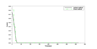
Figure 1: Optimal control with direct and indirect approaches.

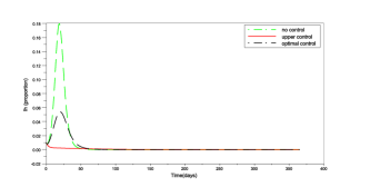
Figure 2: Infected humans using different levels of control.

Method	optimal control	no control ($u\equiv 0$)	upper control ($u\equiv 1$)
Direct (DOTcvpSB)	0.146675	0.674555	364.940488
Indirect (backward-forward)	0.113137	0.357285	365.00046

Table 1: Values of the cost functional (2)

Table 1 shows the costs obtained by the two methods, in three situations: optimal control, no control ($u(t)\equiv 0$) and upper control ($u(t)\equiv 1$). Figure 2 shows the number of infected humans when different controls are considered. It is possible to see that the upper control, which means that everyone is vaccinated, implies that just a few individuals were infected, allowing eradication of the disease. Although the optimal control, in the sense of objective (2), allows the occurrence of an outbreak, the number of infected individuals is much lower when compared with a situation where no one is vaccinated. Also, the costs are very low when compared with the upper control case.

4 Conclusions

Dengue is an infectious tropical disease difficult to prevent and manage. Researchers agree that the development of a vaccine for dengue is a question of high priority. In the present study we show how a vaccine results in saving lives and at the same time in a reduction of the budget related with the disease. As future work we intend to study the interaction of a dengue vaccine with other kinds of control already investigated in the literature, such as insecticide and educational campaigns [8, 9].

References

- [1] P. Cattand, P. Desjeux, M. G. Guzmán, J. Jannin, A. Kroeger, A. Medici, P. Musgrove, M. B. Nathan, A. Shaw, and C. J. Schofield, Tropical Diseases Lacking Adequate Control Measures: Dengue, Leishmaniasis, and African Trypanosomiasis, Disease Control Priorities in Developing Countries, 2nd edition, DCPP Publications, Washington (DC), 451–466 (2006).
- [2] S. Murrel, S.-C. Wu, and M. Butler, Biotechnology Advances 29, 239–247 (2011).
- [3] L. S. Pontryagin, V. G. Boltyanskii, R. V. Gamkrelidze, and E. F. Mishchenko, The mathematical theory of optimal processes, A Pergamon Press Book. The Macmillan Co., New York, 1964.
- [4] J. T. Betts, Practical methods for optimal control and estimation using nonlinear programming, vol. 19 of Advances in Design and Control, Society for Industrial and Applied Mathematics (SIAM), Philadelphia, PA, 2010, second edn.
- [5] E. Trélat, Contrôle optimal, Mathématiques Concrètes. [Concrete Mathematics], Vuibert, Paris, 2005.
- [6] T. Hirmajer, E. Balsa-Canto, and J. R. Banga, BMC Bioinformatics 10, 199–213 (2009).
- [7] S. Lenhart, and J. T. Workman, Optimal control applied to biological models, Chapman & Hall/CRC, 2007.
- [8] H. S. Rodrigues, M. T. T. Monteiro, and D. F. M. Torres, “Insecticide control in a Dengue epidemics model”, in Numerical Analysis and Applied Mathematics, edited by T. Simos, AIP Conf. Proc. 1281, 979–982 (2010). arXiv:1007.5159
-
[9]
H. S. Rodrigues, M. T. T. Monteiro, D. F. M. Torres, and A. Zinober,
Dengue disease, basic reproduction number and control,
Int. J. Comput. Math. (2011), in press.
DOI: 10.1080/00207160.2011.554540 arXiv:1103.1923