Two-photon Indirect Optical Injection and Two-color Coherent Control in Bulk Silicon

Abstract

Using an empirical pseudopotential description of electron states and an adiabatic bond charge model for phonon states in bulk silicon, we theoretically investigate two-photon indirect optical injection of carriers and spins and two-color coherent control of the motion of the injected carriers and spins. For two-photon indirect carrier and spin injection, we identify the selection rules of band edge transitions, the injection in each conduction band valley, and the injection from each phonon branch at 4 K and 300 K. At 4 K, the TA phonon-assisted transitions dominate the injection at low photon energies, and the TO phonon-assisted at high photon energies. At 300 K, the former dominates at all photon energies of interest. The carrier injection shows anisotropy and linear-circular dichroism with respect to light propagation direction. For light propagating along the $\langle 001\rangle$ direction, the carrier injection exhibits valley anisotropy, and the injection into the $Z$ conduction band valley is larger than that into the $X/Y$ valleys. For $\sigma^{-}$ light propagating along the $\langle 001\rangle$ ($\langle 111\rangle$) direction, the degree of spin polarization gives a maximum value about $20\%$ ($6\%$) at 4 K and $-10\%$ ($20\%$) at 300 K, and at both temperature shows abundant structure near the injection edges due to contributions from different phonon branches. For the two-color coherent current injection with an incident optical field composed of a fundamental frequency and its second harmonic, the response tensors of the electron (hole) charge and spin currents are calculated at 4 K and 300 K. We show the current control for three different polarization scenarios: For co-circularly polarized beams, the direction of the charge current and the polarization direction of the spin current can be controlled by a relative-phase parameter; for the co-linearly and cross-linearly polarized beams, the current amplitude can be controlled by that parameter. The spectral dependence of the maximum swarm velocity shows that the direction of charge current reverses under increase in photon energy.

I Introduction

Silicon is a dominant material in the microelectronics industry. It has also attracted much attention in optoelectronicsSiliconPhotonics_Lockwood_Pavesi ; IEEE_12_1678_2006_Soref ; J.LightwaveTech._23_4222_2005_Lipson , due to its low absorption at telecommunication wavelengths near $1.55~{}\mu$m, and in spintronicsRev.Mod.Phys._76_323_2004_Zutic ; ActaPhys.Slovaca_57_565_2007_Fabian ; Phys.Rep._493_61_2010_Wu , due to its long spin transport length and spin relaxation timeNature_447_295_2007_Appelbaum ; Phys.Rev.Lett._99_177209_2007_Huang ; NaturePhys._3_542_2007_Jonker ; Phys.Rev.B_2_2429_1970_Lepine ; Phys.Rev.B_78_054446_2008_Mavropoulos ; Phys.Rev.B_79_075303_2009_Zhang ; Phys.Rev.Lett._105_037204_2010_Li . In both fields, a full understanding of the optical properties in bulk silicon is very important for further applications. Optical methods can provide an effective way to generate carriers and spins in semiconductors, to controlPhys.StatusSolidiB_243_2278_2006_vanDriel ; CoherentControlOfPhotocurrentsinSemiconductors_Driel ; CoherentControl_Driel their motions by the phase coherence of different components of incident laser beams, and to detect the properties of carriers and spinsoptical_orientation . Recently, the direct detection of spin currents using second-order nonlinear optical effects has been proposedPhys.Rev.Lett._104_256601_2010_Wang and realized experimentallyNat.Phys._6_875_2010_Werake .

Because silicon is an indirect gap semiconductor, with an indirect gap $E_{ig}=1.17$ eV and a direct gap $E_{g}=3.4$ eV landolt_Si , there is a degenerate indirect “$\ell$”-photon optical transition assisted by phonon emission or absorption at $\ell\hbar\omega<E_{g}$. This optical response is about two orders of magnitude weaker than that in direct gap semiconductors. While the weak response results in low loss, which is important in realizing optoelectronics devices, it can make optical coherent control less effective.

By using circularly polarized light, spin polarized carriers can be injectedoptical_orientation . Generally, one- and two-photon injection are the most widely used schemes. For coherent current control, the minimum requirements depend on the semiconductor crystal structures: For low symmetry semiconductor structures with nonvanishing second order nonlinearity, such as the wurtzite structureAppl.Phys.Lett._75_2581_1999_Laman , current can be injected by even a single frequency laser beam; for high symmetry semiconductor structures with vanishing second order nonlinearity but non-vanishing third-order nonlinearity, such as the diamond structures, current injection requires at least a two-color laser pulse with one fundamental frequency and its $\ell^{th}$ harmonic (“$1+\ell$” effects). The control parameters are taken as a relative-phase parameter between Cartesian components or between the frequency components of the two-color laser beams. However, most coherent control studies to date have focused on absorption across the direct gapAppl.Phys.Lett._95_092107_2009_Loren ; Phys.Rev.Lett._85_5432_2000_Bhat ; Phys.Rev.B_68_165348_2003_Najmaie , even when considering the indirect gap semiconductorsPhys.Rev.B_81_155215_2010_Rioux ; seldom has coherent control by absorption across an indirect gap been consideredAppl.Phys.Lett._97_212106_2010_Zhao ; NaturePhys._3_632_2007_Costa ; Phys.Rev.B_77_085201_2008_Spasenovic , due to the weak optical response. For silicon, which has diamond structure and vanishing second-order nonlinearity, it is only the second of the coherent control schemes mentioned above that is applicable.

For two-photon indirect optical carrier injection in bulk silicon, most experimental studies have focused on the two-photon absorption coefficientPhys.Rev.Lett._30_901_1973_Reintjes ; Appl.Phys.Lett._80_416_2002_Tsang ; Appl.Phys.Lett._82_2954_2003_Dinu ; Appl.Phys.Lett._90_191104_2007_Bristow ; Appl.Phys.Lett._91_071113_2007_Zhang ; Appl.Phys.Lett._91_021111_2007_Lin and its anisotropyAppl.Phys.Lett._91_071113_2007_Zhang , which is important in optoelectronics devices; theoretical studiesIEEEJ.QuantumElectron._39_1398_2003_Dinu ; J.Phys.B_39_2737_2006_Garcia ; Phys.Stat.Solidi(b)_184_519_1994_Hassan ; Phys.Stat.Solidi(b)_186_303_1994_Hassan are mostly based on the parabolic band approximation and on a phenomenological electron-phonon interaction. For the current injection by coherent control, Costa et al.NaturePhys._3_632_2007_Costa and Spasenović et al. Phys.Rev.B_77_085201_2008_Spasenovic used THz radiation to detect “1+2” injected current in bulk silicon, and confirmed that the current can be controlled by the phase parameter of the laser beams. Zhao and Smirl Appl.Phys.Lett._97_212106_2010_Zhao measured the time- and space-evolution of the indirect optical injected electrons and holes by phase-dependent differential transmission techniques. Yet a full band structure investigations of the two-photon indirect optical injection of spins and spin current are still lacking.

Previously we studied the one-photon indirect optical injection of carriers and spinsPhys.Rev.B_83_165211_2011_Cheng , and the spectral dependence of the two-photon indirect absorption coefficients and their phonon-resolved injection rates at 4 K and 300 KAppl.Phys.Lett._98_131101_2011_Cheng . In this paper, we continue the study of the two-photon indirect optical injection of carriers and spins, and consider as well the coherent control of the injected charge and spin currents by “1+2” effects. We present the detailed results of two-photon indirect carrier and spin injection under $\sigma^{-}$ light propagating along $\langle 001\rangle$ and $\langle 111\rangle$ directions; due to the symmetries of bulk silicon, the injection with $\sigma^{+}$ light has the same carrier and spin injection as with $\sigma^{-}$ light, but with the opposite spin polarization. The injection in each conduction band valley, the anisotropy and the linear-circular dichroism with respect to light propagation direction, the corresponding phonon-resolved spectra, and the degree of spin polarization (DSP) are discussed. We also consider the coherent control of the motion of optically injected electrons and holes under particular two-color optical fields: co-circularly polarized beams, co-linearly polarized beams, and cross-linearly polarized beams.

In optical absorption, the electron-hole interaction plays an important role especially in determining the correct absorption edges. First principle studiesPhys.Rev.B_62_4927_2000_Rohlfing of the direct gap optical absorption shows that the excitonic effect can strongly change the lineshape even for high photon energies in silicon. For indirect one-Phys.Rev._108_1384_1957_Elliott and two-photon injectionPhys.Stat.Solidi(b)_184_519_1994_Hassan ; Phys.Stat.Solidi(b)_186_303_1994_Hassan , investigations within the parabolic band approximation show that this neglect does not change the absorption lineshapes at energies more than a few binding energies above the band gap; however, a full band structure investigation is still lacking due to difficulty in numerical calculation of the wave functions of the electron-hole pair. In this paper, as a preliminary calculation, we neglect the excitonic effect.

We organize the paper as follows. Two-photon indirect carrier and spin injection are presented in Sec. II. In this section, we first describe a perturbation model for two-photon indirect optical injection, and then give the numerical results under an empirical pseudopotential model for electronic states and an adiabatic bond charge model for phonon states. In Sec. III, we study the interference current injection under a two-color laser beam and the coherent control. We conclude in Sec. IV.

II Two-photon indirect Carrier and spin injection

II.1 Model for two-photon indirect injection

For an incident laser beam with electric field ${\bm{E}}(t)={\bm{E}}_{\omega}e^{-i\omega t}+c.c$, the two-photon optical injection rates of electrons and their spins are generally written as

$$\dot{n} = \xi^{abcd}E_{\omega}^{a}E_{\omega}^{b}(E_{\omega}^{c}E_{\omega}^{d})^{\ast}\ ,$$

$$\dot{S}^{f} = \zeta^{fabcd}E_{\omega}^{a}E_{\omega}^{b}(E_{\omega}^{c}E_{\omega}^{d})^{\ast}\ ,$$ (1)

From these rates, the actual injected carrier density and spin density can be calculated once the pulse duration is specified. In this paper, superscripts indicate Cartesian coordinates, and repeated superscripts are to be summed over. For bulk silicon, the lowest conduction band has six equivalent valleys, which are usually denoted as $X,\bar{X},Y,\bar{Y},Z,\bar{Z}$. The two-photon indirect transitions have the same initial and final states as that of one-photon indirect transitionsPhys.Rev.B_83_165211_2011_Cheng . The injection coefficients can be written as the form ${\cal A}^{abcd}=\sum_{I}{\cal A}^{abcd}_{I}$ with ${\cal A}^{abcd}_{I}$ identifying the injection into the $I^{th}$ valley. Fermi’s golden rule gives ${\cal A}^{abcd}_{I}=\sum_{cv\lambda\pm}{\cal A}^{abcd}_{I;cv\lambda\pm}$ with

$${\cal A}^{abcd}_{I;cv\lambda\pm} = \frac{2\pi}{\hbar}\sum_{\bm{k}_{c}\in I,\bm{k}_{v}}\delta(\varepsilon_{c\bm{k}_{c}}-\varepsilon_{v\bm{k}_{v}}\pm\hbar\Omega_{(\bm{k}_{c}-\bm{k}_{v})\lambda}-2\hbar\omega)$$ (2)

$$\times N_{(\bm{k}_{c}-\bm{k}_{v})\lambda\pm}{\cal A}^{abcd}_{c\bm{k}_{c}v\bm{k}_{v}\lambda}\ ,$$

$${\cal A}^{abcd}_{c\bm{k}_{c}v\bm{k}_{v}\lambda}=\sum_{\sigma_{c}\sigma_{c}^{\prime}\sigma_{v}}\langle\bar{c}^{\prime}\bm{k}_{c}|\hat{\cal A}|\bar{c}\bm{k}_{c}\rangle W^{ab}_{\bar{c}\bm{k}_{c}\bar{v}\bm{k}_{v}\lambda}[W^{cd}_{\bar{c}^{\prime}\bm{k}_{c}\bar{v}\bm{k}_{v}\lambda}]^{\ast}\ .$$ (3)

The coefficient ${\cal A}^{abcd}_{I;cv\lambda\pm}$ gives the contribution to the injection by indirect optical transition between conduction band $c$ and valence band $v$, with the assistance of an emitted ($+$) or absorbed ($-$) phonon in the $\lambda^{th}$-mode; there are two modes each for the transverse acoustic (TA) and optical (TO) branches, and one mode each for the longitudinal acoustic (LA) and optical (LO) branches. The operator $\hat{A}$ in Eq. (3) stands for the identity operator in carrier injection, and the $f^{th}$ component of spin operator in spin injection. The optical transition matrix elements are given as

$$W^{ab}_{\bar{c}\bm{k}_{c}\bar{v}\bm{k}_{v}\lambda} = \frac{1}{2}\left(\frac{e}{\hbar\omega}\right)^{2}\sum_{\bar{n}\bar{m}}\bigg{[}\frac{M_{\bar{c}\bm{k}_{c}\bar{n}\bm{k}_{v};\lambda}v^{a}_{\bar{n}\bar{m}\bm{k}_{v}}v^{b}_{\bar{m}\bar{v}\mathbf{k}_{v}}}{(\omega_{nv\bm{k}_{v}}-2\omega)(\omega_{mv\mathbf{k}_{v}}-\omega)}$$ (4)

$$- \frac{v^{a}_{\bar{c}\bar{n}\bm{k}_{c}}M_{\bar{n}\bm{k}_{c}\bar{m}\bm{k}_{v};\lambda}v^{b}_{\bar{m}\bar{v}\bm{k}_{v}}}{(\omega_{cn\bm{k}_{c}}-\omega)(\omega_{mv\bm{k}_{v}}-\omega)}$$

$$+ \frac{v^{a}_{\bar{c}\bar{n}\bm{k}_{c}}v^{b}_{\bar{n}\bar{m}\bm{k}_{c}}M_{\bar{m}\bm{k}_{c}\bar{v}\bm{k}_{v};\lambda}}{(\omega_{cn\bm{k}_{c}}-\omega)(\omega_{cm\bm{k}_{c}}-2\omega)}\bigg{]}+\{a\leftrightarrow b\}$$

where $e=|e|$. Here $\bm{k}_{c}$ and $\bm{k}_{v}$ are the electron and hole wave vectors respectively; $\bar{c}=\{c,\sigma_{c}\}$, $\bar{c}^{\prime}=\{c,\sigma_{c}^{\prime}\}$, and $\bar{v}=\{v,\sigma_{v}\}$ are full band indexes with $\sigma_{c}$, $\sigma_{c}^{\prime}$ and $\sigma_{v}$ being the spin indexes; $\bar{n}$ and $\bar{m}$ are band indices for intermediate states; $|\bar{c}\bm{k}_{c}\rangle$ and $\varepsilon_{c\bm{k}_{c}}$ are the electron states and its energy respectively; and $\omega_{nm}(\bm{k})$ is defined as $\hbar\omega_{nm}(\bm{k})=\varepsilon_{n\bm{k}}-\varepsilon_{m\bm{k}}$. The phonon energy is given by $\hbar\Omega_{\bm{q}\lambda}$ for wavevector $\bm{q}$ and mode $\lambda$, the equilibrium phonon number is $N_{\bm{q}\lambda}$, and $N_{\bm{q}\lambda\pm}=N_{\bm{q}\lambda}+\frac{1}{2}\pm\frac{1}{2}$. The velocity matrix elements are $\bm{v}_{\bar{n}\bar{m}}(\bm{k})=\langle\bar{n}\bm{k}|\hat{\bm{v}}|\bar{m}\bm{k}\rangle$ with the velocity operator $\hat{\bm{v}}=\partial H_{e}/\partial\bm{p}$, and $H_{e}$ is the unperturbed electron Hamiltonian. The electron-phonon interaction is written as $H^{ep}=\sum_{\bm{q}\lambda}H_{\lambda}^{ep}(\bm{q})(a_{\bm{q}\lambda}+a_{-\bm{q}\lambda}^{{\dagger}})$ with $a_{\bm{q}\lambda}$ standing for the phonon annihilation operator. Its matrix elements are $M_{\bar{n}\bm{k}_{c}\bar{m}\bm{k}_{v}\lambda}=\langle\bar{n}\bm{k}_{c}|H^{ep}_{\lambda}(\bm{k}_{c}-\bm{k}_{v})|\bar{m}\bm{k}_{v}\rangle$.

The injection coefficient $\xi^{abcd}_{I}$ is a fourth-order tensor and $\zeta^{fabcd}_{I}$ is a fifth-order pseudotensor. Both of them are symmetric on exchange of indices $a$ and $b$, and on exchange of indices $c$ and $d$. They have the properties $\left(\xi^{abcd}_{I}\right)^{\ast}=\xi_{I}^{cdab}$ and $\left(\zeta^{fabcd}_{I}\right)^{\ast}=\zeta_{I}^{fcdab}$. Furthermore, time-reversal symmetry gives $\xi_{I}^{abcd}=\left(\xi_{\bar{I}}^{abcd}\right)^{\ast}$ and $\zeta_{I}^{fabcd}=-\left(\zeta_{\bar{I}}^{fabcd}\right)^{\ast}$. In bulk silicon, each conduction band valley has $C_{4v}$ symmetry. Under this symmetry, $\xi_{Z}^{abcd}$ has six nonzero independent components,

$$\xi^{xxxx}_{Z} = \xi^{yyyy}_{Z}\ ,$$

$$\xi^{xxyy}_{Z} = \xi^{yyxx}_{Z}\ ,$$

$$\xi^{zzxx}_{Z} = \xi^{zzyy}_{Z}\ ,$$

$$\xi^{xyxy}_{Z} \ ,$$

$$\xi^{xzxz}_{Z} = \xi^{yzyz}\ ,$$

$$\xi^{zzzz}_{Z} \ ;$$ (5)

$\zeta_{Z}^{fabcd}$ also has six nonzero independent components,

$$\zeta_{Z}^{zxyxx} = -\zeta_{Z}^{zxyyy}\ ,$$

$$\zeta_{Z}^{zyzxz} = -\zeta_{Z}^{zxzyz}\ ,$$

$$\zeta_{Z}^{xyzyy} = -\zeta_{Z}^{yxzxx}\ ,$$

$$\zeta_{Z}^{xyzxx} = -\zeta_{Z}^{yxzyy}\ ,$$

$$\zeta_{Z}^{xxzxy} = -\zeta_{Z}^{yyzxy}\ ,$$

$$\zeta_{Z}^{xzzyz} = -\zeta_{Z}^{yzzxz}\ .$$ (6)

The injection coefficients ${\cal A}^{abcd}_{I}$ can be obtained by a proper rotation operation that transforms the $Z$ valley to the $I^{th}$ valley. Using inversion and time-reversal symmetries, all $\xi^{abcd}$ are identified as real numbers, and all $\zeta^{fabcd}$ are pure imaginary numbers; ${\cal A}^{abcd}_{I;cv\lambda\pm}$ shares the same symmetry properties as ${\cal A}^{abcd}_{I}$, while ${\cal A}^{abcd}$ belongs to the higher symmetry group $O_{h}$, and has fewer nonzero independent components

$$\xi^{xxxx}=\xi^{yyyy}=\xi^{zzzz}\ ,$$

$$\xi^{xxyy}=\xi^{xxzz}=\xi^{yyzz}=\xi^{yyxx}=\xi^{zzxx}=\xi^{zzyy}\ ,$$

$$\xi^{xyxy}=\xi^{xzxz}=\xi^{yzyz}\ ,$$ (7)

and

$$\zeta^{zxyxx}=-\zeta^{zyxyy}=\zeta^{yzxzz}$$

$$\quad\quad\quad=-\zeta^{yxzxx}=\zeta^{xyzyy}=-\zeta^{xzyzz}\ ,$$

$$\zeta^{xxzxy}=-\zeta^{xyxxz}=\zeta^{yxyyz}$$

$$\quad\quad\quad=-\zeta^{yzyyx}=\zeta^{zyzxz}=-\zeta^{zzxyz}\ .$$ (8)

All these components are related to the nonzero injection coefficients in the $Z$ valley by

$$\xi^{xxxx} = 4\xi_{Z}^{xxxx}+2\xi_{Z}^{zzzz}\ ,$$

$$\xi^{xxyy} = 4\xi_{Z}^{zzxx}+2\xi_{Z}^{xxyy}\ ,$$

$$\xi^{xyxy} = 4\xi_{Z}^{xzxz}+2\xi_{Z}^{xyxy}\ ,$$

$$\zeta^{xxzxy} = 4\zeta_{Z}^{xxzxy}+2\zeta_{Z}^{zyzxz}\ ,$$

$$\zeta^{zxyxx} = 2\zeta_{Z}^{zxyxx}+2\zeta_{Z}^{xzzyz}+2\zeta_{Z}^{xyzyy}\ .$$ (9)

With all these coefficients, the injection rates for laser pulse with any polarization and propagating directions can be evaluated. In Appendix A, we give in detail the carrier and spin injection rates for circularly-polarized light with any propagating direction, and the carrier injection rates for linearly-polarized light with any polarization and propagating directions. In the following, we focus on light propagating along $\langle 001\rangle$ and $\langle 111\rangle$ directions.

II.2 Results

For quantitative calculations of the two-photon indirect injection rates, a full band-structure description of the electron and phonon states is necessary. Here we use an empirical pseudopotential modelPhys.Rev.B_10_5095_1974_Chelikowsky ; Phys.Rev.B_14_556_1976_Chelikowsky ; Phys.Rev._149_504_1966_Weisz for electron states and an adiabatic bond charge modelPhys.Rev.B_15_4789_1977_Weber for phonon states. All the parameters used in the empirical pseudopotential model and the adiabatic bond charge model are the same as those in the calculation of one-photon optical spin injectionPhys.Rev.B_83_165211_2011_Cheng . From the empirical pseudopotential model, the calculated direct band gap is $E_{g}=3.43$ eV, the indirect band gap is $E_{ig}=1.17$ eV; the band edge for the conduction band is located at $\bm{k}_{c}^{0}=0.85~{}\overrightarrow{\Gamma X}$, and for the valence bands at the $\Gamma$ point, $\bm{k}_{v}^{0}=0$. From the adiabatic bond charge model, the energies for phonons with wavevector $\bm{k}_{c}^{0}$ are $19$ (TA), $43$ (LA), $53$ (LO), and $57$ (TO) meV. Within the pseudopotential scheme we determine the electron-phonon interaction, and then evaluate the matrix elements $H_{\lambda}^{ep}(\bm{q})$ using the calculated electron and phonon wavefunctions. With all these quantities calculated, the two-photon indirect gap transition matrix elements in Eq. (4) are calculated using the lowest $30$ electron bands as intermediate states to ensure convergence. The injection coefficients given in Eq. (3) are evaluated using an improved linear analytic tetrahedral methodPhys.Rev.B_83_165211_2011_Cheng .

In our calculation, the valence bands include heavy hole (HH), light hole (LH), and spin split-off (SO) bands; the conduction bands include the lowest two conduction bands. Our results are shown in Fig. 1 for the spectra of nonzero components of $\xi^{abcd}_{Z}$ and in Fig. 2 for the spectra of nonzero components of $\zeta^{fabcd}_{Z}$ at 4 K and 300 K, respectively. The full two-photon indirect gap injection rates in Eq. (1) can be identified for any polarization of the electric field using Eq. (9). Comparing the injection rates given in Eqs. (2) and (3) with the one-photon indirect optical injection ratesPhys.Rev.B_83_165211_2011_Cheng , we find that these two formulas differ only in the transition matrix elements given in Eq. (3). Therefore they show similar temperature dependence, which is mainly determined by the phonon number, and similar contributions from each valence band, which is mainly determined by the joint density of states.

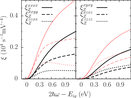
Figure 1: (Color online) Spectra of $\xi_{Z}^{abcd}$ at 4 K (thick black curves) and 300 K (thin red curves).

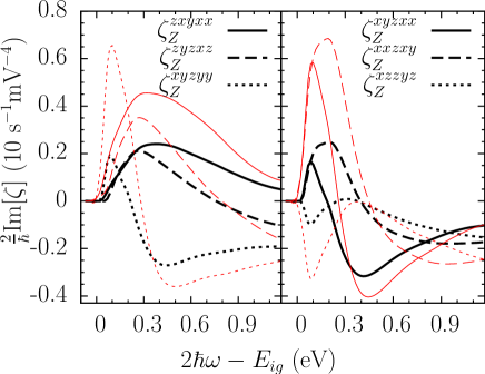
Figure 2: (Color online) Spectra of $\frac{2}{\hbar}\text{Im}[\zeta_{Z}^{fabcd}]$ at 4 K (thick black curves) and 300 K (thin red curves).

In a previous paperAppl.Phys.Lett._98_131101_2011_Cheng , we discussed in detail the photon energy, temperature, and phonon branch dependence of the total carrier injection coefficients $\xi^{xxxx}$, $\xi^{xxyy}$, and $\xi^{xyxy}$. Here the $\xi^{abcd}_{Z}$ in Fig. 1 show similar properties: For excess photon energies $2\hbar\omega-E_{ig}$ of interest, $\xi_{Z}^{zzxx}$ first increases with increasing photon energy, and then slightly decreases; all the other components increase monotonically. In contrast, all the components of $\zeta^{fabcd}_{Z}$, given in Fig. 2, show a complicated photon energy dependence. All injection rates at 300 K are larger than those at 4 K due to the larger phonon populations.

To better understand these results, we first consider the properties of transitions around the band edges. Then we turn to the injection rates of carriers and spins, and the DSP under $\sigma^{-}$ light propagating along two different directions.

II.2.1 Transitions near band edges

One can try to simplify the description of the indirect two-photon injection around the band edges using the high symmetry at the band edge. We symmetrize the indirect two-photon injection rates as

$${\cal A}^{abcd}_{I;cv\tau\pm} = \frac{2\pi}{\hbar}\sum_{\bm{k}_{c}\in I\atop\bm{k}_{v},\lambda\in\tau}\frac{1}{{\cal N}_{v}}\sum_{P_{v}}\delta(\varepsilon_{c\bm{k}_{c}}-\varepsilon_{v\bm{k}_{v}}\pm\hbar\Omega_{(\bm{k}_{c}-P_{v}\bm{k}_{v})\lambda}$$ (10)

$$- \hbar\omega)N_{(\bm{k}_{c}-P_{v}\bm{k}_{v})\lambda\pm}\tilde{\cal A}^{abcd}_{I;c\bm{k}_{c}v(P_{v}\bm{k}_{v})\lambda}\ .$$

Here $\tilde{\cal A}^{abcd}_{I;c\bm{k}_{c}v\bm{k}_{v}\lambda}=\sum_{P_{c,I}}{\cal A}^{abcd}_{c(P_{c,I}\bm{k}_{c})v(P_{c,I}\bm{k}_{v})\lambda}/{\cal N}_{c,I}$; $P_{c,I}$ are the ${\cal N}_{c,I}$ symmetry operations in $C_{4v}$ that keep the $I^{th}$ valley unchanged, while $P_{v}$ are the ${\cal N}_{v}$ symmetry operations in $O_{h}$; and $\sum_{\lambda\in\tau}$ indicates summation over all modes in the $\tau^{th}$ branch. Around the band edge, it is a good approximation to take the mediated phonon energy $\hbar\Omega_{(\bm{k}_{c}-\bm{k}_{v})\lambda}$ and the phonon number $N_{(\bm{k}_{c}-\bm{k}_{v})\lambda}$ to be constant and equal to their band edge values $\hbar\Omega_{\bm{k}_{c}^{0}\lambda}=\hbar\Omega^{0}_{\tau}$ and $N_{\bm{k}_{c}^{0};\lambda}=N_{\tau}^{0}$ , respectively. Then the injection rates are approximately

$${\cal A}^{abcd}_{I;cv\tau\pm}=\frac{2\pi}{\hbar}\sum_{\bm{k}_{c}\in I\atop\bm{k}_{v}}\delta(\varepsilon_{c\bm{k}_{c}}-\varepsilon_{v\bm{k}_{v}}\pm\hbar\Omega^{0}_{\tau}-\hbar\omega)N^{0}_{\tau\pm}\bar{\cal A}^{abcd}_{I;c\bm{k}_{c}v\bm{k}_{v}\tau}\ ,$$ (11)

with

$$\bar{\cal A}^{abcd}_{I;c\bm{k}_{c}v\bm{k}_{v}\tau} = \frac{1}{{\cal N}_{v}}\sum_{P_{v},\lambda\in\tau}\tilde{\cal A}^{abcd}_{I;c\bm{k}_{c}v(P_{v}\bm{k}_{v})\lambda}\ .$$ (12)

Here the symmetrized expression $\bar{\cal A}^{abcd}_{I;c\bm{k}_{c}v\bm{k}_{v}\tau}$ in Eq. (11) avoids the ambiguity in calculating the band edge values of ${\cal A}_{c\bm{k}_{c}v\bm{k}_{v}\lambda}^{abcd}$, which is induced by the degeneracy of the heavy and light hole bands at the $\Gamma$ points. This can be clearly shown by rewriting $W^{ab}_{\bar{c}\bm{k}_{c}\bar{v}\bm{k}_{v}\lambda}=\langle\bar{c}\bm{k}_{c}|\hat{W}^{ab}_{c\bm{k}_{c}v\bm{k}_{v}\lambda}+\hat{W}^{ba}_{c\bm{k}_{c}v\bm{k}_{v}\lambda}|\bar{v}\bm{k}_{v}\rangle$ with the operator

$$\hat{W}^{ab}_{c\bm{k}_{c}v\bm{k}_{v}\lambda} \equiv \frac{1}{2}(\frac{e}{\omega})^{2}\bigg{[}H_{\lambda}^{ep}(\bm{k}_{c}-\bm{k}_{v})\frac{1}{H_{e}-\varepsilon_{v\bm{k}_{v}}-2\hbar\omega}$$

$$\times\hat{v}^{a}\frac{1}{H_{e}-\varepsilon_{v\bm{k}_{v}}-\bar{\omega}}\hat{v}^{b}-\hat{v}^{a}\frac{1}{\varepsilon_{c\bm{k}_{c}}-H_{e}-\hbar\omega}$$

$$\times H_{\lambda}^{ep}(\bm{k}_{c}-\bm{k}_{v})\frac{1}{H_{e}-\varepsilon_{v\bm{k}_{v}}-\hbar\omega}\hat{v}^{b}+\hat{v}^{a}$$

$$\times\frac{1}{\varepsilon_{c\bm{k}_{c}}-H_{e}-\hbar\omega}\hat{v}^{b}\frac{1}{\varepsilon_{c\bm{k}_{c}}-H_{e}-2\hbar\omega}H_{\lambda}^{ep}(\bm{k}_{c}-\bm{k}_{v})\bigg{]}\ ,$$

keeping the intermediate states appearing in Eq. (4) implicit. Then similar to the corresponding results for one-photon indirect optical transitionPhys.Rev.B_83_165211_2011_Cheng , we have

$$\bar{\cal A}^{abcd}_{I;c\bm{k}_{c}^{0}\text{HH}\bm{k}_{v}^{0}\tau}=\bar{\cal A}^{abcd}_{I;c\bm{k}_{c}^{0}\text{LH}\bm{k}_{v}^{0}\tau}=\frac{1}{2}\sum_{v^{\prime}=\text{LH},\text{HH}}\bar{\cal A}^{abcd}_{I;c\bm{k}_{c}^{0}v^{\prime}\bm{k}_{v}^{0}\tau}\ ,$$ (13)

which is unambiguous for any choice of heavy and light hole state at the valence band edge. We analyze the nonzero matrix elements of $\bar{\cal A}^{abcd}_{I;c\bm{k}_{c}^{0}v\bm{k}_{v}^{0}\tau}$ using the symmetries of the crystal.

For a given symmetry operation, the transformation of $\hat{W}^{ab}$ is determined by $H^{ep}_{\lambda}$, $\hat{v}^{a}$, and $\hat{v}^{b}$; a direct symmetry analysis for $W^{ab}_{\bar{c}\bm{k}_{c}^{0}\bar{v}\bm{k}_{v}^{0}\lambda}$ is possible with the electron state $|\bar{c}\bm{k}_{c}^{0}\rangle$ and the hole state $|\bar{v}\bm{k}_{v}^{0}\rangle$. However, because of very weak spin orbit coupling in silicon, this process can be greatly simplified by dropping spin orbit coupling terms in $H^{ep}_{\lambda}$, $\hat{v}^{a}$, and $\hat{v}^{b}$, and thus in $\hat{W}^{ab}_{c\bm{k}_{c}v\bm{k}_{v}\lambda}$. Without spin-orbit coupling, the valence states at $\Gamma$ are chosen with the symmetry properties of $\{{\cal X}=yz,{\cal Y}=zx,{\cal Z}=xy\}$; the phonon states are chosen with the symmetry $\{x,y\}$ for TA/TO branch, $\{z\}$ for LA branch, and $\{x^{2}-y^{2}\}$ for LO branch; without losing generality, the conduction band edge states are taken to lie in the $Z$ valley, which has the symmetry of $\{z\}$. All matrix elements are listed in Table 1. In total there are fifteen nonzero quantities for the band edge values. From the table, selection rules depend strongly on phonon states.

With spin orbit coupling, the valence bands are split into HH ($|\frac{3}{2},\pm\frac{3}{2}\rangle$), LH ($|\frac{3}{2},\pm\frac{1}{2}\rangle$) and SO ($|\frac{1}{2},\pm\frac{1}{2}\rangle$) bands, and the conduction bands are two-fold spin degenerate bands $|z\uparrow\rangle$ and $|z\downarrow\rangle$. The indirect optical matrix elements in these states can be easily obtained by linear combination of the terms in Table 1, and the band edge transition probabilities can be identified by $\bar{\cal A}^{abcd}_{Z;cv\tau}=\bar{\cal A}^{abcd}_{c\bm{k}_{c}^{0}v\bm{k}_{v}^{0}\lambda}$, with $\bm{k}_{c}^{0}$ being the band edge wave vector in the $Z$ valley. Similar to the corresponding term for one-photon absorptionPhys.Rev.B_83_165211_2011_Cheng , $\bar{\cal A}^{abcd}_{Z;cv\tau}$ has the following properties: i) $\bar{\xi}^{abcd}_{Z;cv\tau}$ are the same for $v=$ HH, LH, and SO; ii) $\sum_{v}\bar{\zeta}^{fabcd}_{Z;cv\tau}=0$ and $\bar{\zeta}^{fabcd}_{Z;c\text{HH}\tau}=\bar{\zeta}^{fabcd}_{Z;c\text{LH}\tau}$.

	TA/TO		LA	LO
$W^{ab}_{c\bm{k}_{c}^{0}v\bm{k}_{v}^{0}\tau}$	$x$	$y$	$z$	$x^{2}-y^{2}$
$|{\cal X}\rangle$	$W_{1}^{(\prime)}M^{12}$	$W_{2}^{(\prime)}M^{11}+W_{3}^{(\prime)}M^{22}+W_{4}^{(\prime)}M^{33}$	$W_{6}M^{23}$	$W_{8}M^{13}$
$|{\cal Y}\rangle$	$W_{2}^{(\prime)}M^{22}+W_{3}^{(\prime)}M^{11}+W_{4}^{(\prime)}M^{33}$	$W_{1}^{(\prime)}M^{12}$	$W_{6}M^{13}$	$W_{8}M^{23}$
$|{\cal Z}\rangle$	$W_{5}^{(\prime)}M^{23}$	$W_{5}^{(\prime)}M^{13}$	$W_{7}M^{12}$	$W_{9}(M^{11}+M^{22})+W_{10}M^{33}$

Table 1: Band edge value of $W^{ab}_{c\bm{k}_{c}^{0}v\bm{k}_{v}^{0}\lambda}$. Here $M^{ij}$ is a matrix with matrix elements $[M^{ij}]_{kl}=(1-\delta_{ij})(\delta_{ik}\delta_{jl}+\delta_{il}\delta_{jk})+\delta_{ij}\delta_{ik}\delta_{il}$. There are totally fifteen parameters $\{W_{i},i=1,\cdots,10\}$ for TA, LA, LO phonon branches and $\{W_{i}^{\prime},i=1,\cdots,5\}$ for the TO phonon branch.

	$\tau$
$\bar{\xi}_{Z;c\text{HH}\tau}^{abcd}$	TA/TO	LA	LO
$\bar{\xi}_{Z}^{xxxx}$	$\frac{2}{3}(|W_{3}^{(\prime)}|^{2}+|W_{2}^{(\prime)}|^{2})$	0	$\frac{2}{3}|W_{9}|^{2}$
$\bar{\xi}_{Z}^{xxyy}$	$\frac{4}{3}\text{Re}[W_{3}^{(\prime)}(W_{2}^{(\prime)})^{\ast}]$	0	$\frac{2}{3}|W_{9}|^{2}$
$\bar{\xi}_{Z}^{zzxx}$	$\frac{2}{3}W_{4}^{(\prime)}(W_{3}^{(\prime)}+W_{2}^{(\prime)})^{\ast}$	0	$\frac{2}{3}W_{10}W_{9}^{\ast}$
$\bar{\xi}_{Z}^{xyxy}$	$\frac{4}{3}|W_{1}^{(\prime)}|^{2}$	$\frac{2}{3}|W_{7}|^{2}$	0
$\bar{\xi}_{Z}^{xzxz}$	$\frac{2}{3}|W_{5}^{(\prime)}|^{2}$	$\frac{2}{3}|W_{6}|^{2}$	$\frac{2}{3}|W_{8}|^{2}$
$\bar{\xi}_{Z}^{zzzz}$	$\frac{4}{3}|W_{4}^{(\prime)}|^{2}$	0	$\frac{2}{3}|W_{10}|^{2}$

Table 2: Independent nonzero components of $\bar{\xi}_{Z;c\text{HH}\tau}^{abcd}$.

	$\tau$
$\bar{\zeta}_{Z;c\text{HH}\tau}^{fabcd}$	TA/TO	LA	LO
$\bar{\zeta}_{Z}^{zxyxx}$	$-\frac{i}{3}W_{1}^{(\prime)}(W_{3}^{(\prime)}-W_{2}^{(\prime)})^{\ast}$	0	0
$\bar{\zeta}_{Z}^{zyzxz}$	0	$-\frac{i}{3}|W_{6}|^{2}$	$\frac{i}{3}|W_{8}|^{2}$
$\bar{\zeta}_{Z}^{xyzyy}$	$\frac{i}{3}W_{5}^{(\prime)}(W_{2}^{(\prime)})^{\ast}$	0	$-\frac{i}{3}W_{8}W_{9}^{\ast}$
$\bar{\zeta}_{Z}^{xyzxx}$	$\frac{i}{3}W_{5}^{(\prime)}(W_{3}^{(\prime)})^{\ast}$	0	$-\frac{i}{3}W_{8}W_{9}^{\ast}$
$\bar{\zeta}_{Z}^{xxzxy}$	$\frac{i}{3}W_{5}^{(\prime)}(W_{1}^{(\prime)})^{\ast}$	$-\frac{i}{3}W_{6}W_{7}^{\ast}$	0
$\bar{\zeta}_{Z}^{xzzyz}$	$-\frac{i}{3}W_{4}^{(\prime)}(W_{5}^{(\prime)})^{\ast}$	0	$\frac{i}{3}W_{10}W_{8}^{\ast}$

Table 3: Independent nonzero components of $\bar{\zeta}_{Z;c\text{HH}\tau}^{fabcd}$.

We list $\bar{\cal A}^{abcd}_{Z;c\text{HH}\tau}$ in Table 2 for carrier injection and Table 3 for spin injection. Generally, these nonzero transition probabilities can be used in Eq. (11) to approximate the $\bar{\cal A}^{abcd}_{I;c\bm{k}_{c}v\bm{k}_{v}\tau}$ around the band edge values, which results in a simple formula

$${\cal A}^{abcd}_{I;cv\tau\pm}\approx\frac{2\pi}{\hbar}J_{cv}(\hbar\omega)N^{0}_{\tau\pm}\bar{\cal A}^{abcd}_{I;cv\tau}\ ,$$ (14)

the analog of which is widely used in the qualitative analysis of one-photon direct and indirect injection even for injection away from the band edge. Here $J_{cv}(\hbar\omega)$ is the joint density of states, $J_{cv}(\hbar\omega)=\sum_{\bm{k}_{c}\in I;\bm{k}_{v}}\delta(\varepsilon_{c\bm{k}_{c}}-\varepsilon_{v\bm{k}_{v}}\pm\hbar\Omega^{0}_{\tau}-\hbar\omega)$. In Fig. 3(a), we give the local properties of $\bar{\xi}_{Z;c\bm{k}_{c}(\text{HH})\bm{k}_{v}\tau}^{xxxx}$ around band edges $(\bm{k}_{c}^{0},\bm{k}_{v}^{0})$; its rapid variation away from the band edge shows that the simple formula (14) may fail.

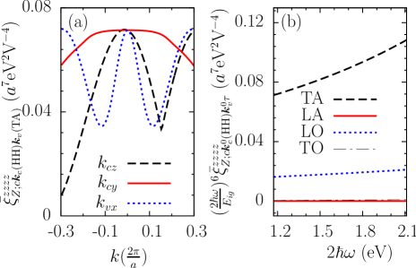
Figure 3: (color online). (a) Values of $\bar{\xi}_{Z;c\bm{k}_{c}(\text{HH})\bm{k}_{v}(\text{TA})}^{zzzz}$ at $2\hbar\omega=E_{ig}$ along different directions: (Dashed black curve) $(\bm{k}_{c}^{0}+k\hat{\bm{z}},\bm{k}_{v}^{0})$, (Solid red curve) $(\bm{k}_{c}^{0}+k\hat{\bm{y}},\bm{k}_{v}^{0})$, and (Dotted blue curve) $(\bm{k}_{c}^{0},\bm{k}_{v}^{0}+k\hat{\bm{x}})$. (b) photon energy dependence of $(2\hbar\omega)^{6}\bar{\xi}_{Z;c\bm{k}_{c}^{0}(\text{HH})\bm{k}_{v}^{0}\tau}^{zzzz}$ for different phonon branches. Here $a=5.431$Å is the lattice constant.

Garcia and KalyanaramanJ.Phys.B_39_2737_2006_Garcia found that the corresponding formula for two photon absorption should be replaced by

$$\beta=\sum_{n\lambda\pm}C_{n\lambda\pm}F_{n}\left(\frac{2\hbar\omega}{E_{ig}},\frac{\pm\hbar\Omega_{\lambda}^{0}}{E_{ig}}\right)\ .$$ (15)

Here the two-photon absorption coefficient $\beta$ is related to our calculated quantity $\xi^{xxxx}$ by $\beta=2\hbar\omega\xi^{xxxx}/(2n_{R}c\epsilon_{0})^{2}$, $n_{R}$ is the refractive index, $c$ is the speed of light, $\epsilon_{0}$ is the vacuum permittivity, $F_{n}(x,y)=(x-y-1)^{2+n}/x^{5}$, and $\Omega_{\lambda}^{0}=\Omega_{\bm{k}_{c}^{0}\lambda}$ is the frequency of phonons mediated in the band edge transitions. According to the parity difference between the band edge hole and electron states, the transitions are divided into allowed-allowed ($a-a$), allowed-forbidden ($a-f$), and forbidden-forbidden ($f-f$) processes, which correspond to the $n=0$, 1, and 2 terms in Eq. (15), respectively; such a classification is based on whether the band edge values of the matrix elements of $v^{a}$ and $v^{b}$ in Eq. (4) are zero (forbidden) or nonzero (allowed) for different parity of the intermediate states. In deriving Eq. (15), the dependence $\xi^{zzzz}_{c\bm{k}_{c}v\bm{k}_{v}\lambda}\propto(\hbar\omega)^{-6}$ must be used. DinuIEEEJ.QuantumElectron._39_1398_2003_Dinu argued instead that $\xi^{zzzz}_{c\bm{k}_{c}v\bm{k}_{v}\lambda}\propto(\hbar\omega)^{-5}$ for some processes. Here we can numerically study this dependence, and the result is plotted in Fig. 3(b); it shows that $\omega^{-5}$ and $\omega^{-6}$ dependences are both important, at least for the TA phonon branch.

The simple formula (14) only corresponds to the $a-a$ process. In obtaining results for the other two processes, the first and second derivatives with respect to $\bm{k}_{c}$ and $\bm{k}_{v}$ of $W^{ab}_{I;c\bm{k}_{c}v\bm{k}_{v}\lambda}$ are necessary. This results in a more complicated symmetry analysis that we do not consider here.

II.2.2 Injection for $\sigma^{-}$ light propagating along $\langle 001\rangle$ and $\langle 111\rangle$

For $\sigma^{-}$ light propagating along the directions $\langle 001\rangle$ and $\langle 111\rangle$, the electric field $\bm{E}^{\langle\hat{\bm{k}}\rangle}$ can be written respectively as

$$\bm{E}^{\langle 001\rangle}_{\omega} = \frac{\hat{\bm{x}}-i\hat{\bm{y}}}{\sqrt{2}}E_{0}\ ,$$

$$\bm{E}^{\langle 111\rangle}_{\omega} = \frac{2i\hat{\bm{x}}+(\sqrt{3}-i)\hat{\bm{y}}-(\sqrt{3}+i)\hat{\bm{z}}}{2\sqrt{3}}E_{0}\ ,$$ (16)

where $\langle\hat{\bm{k}}\rangle$ denotes $\langle 001\rangle$ or $\langle 111\rangle$. The injection rates of carriers and spins then are

$$\dot{n}_{I;cv\lambda\pm} = \xi^{\langle\hat{\bm{k}}\rangle}_{I;cv\lambda\pm}|E_{0}|^{4}\ ,$$

$$\dot{S}^{f}_{I;cv\lambda\pm} = \zeta^{f;\langle\hat{\bm{k}}\rangle}_{I;cv\lambda\pm}|E_{0}|^{4}\ .$$ (17)

Here $\xi_{I}^{\langle\hat{\bm{k}}\rangle}$ and $\zeta_{I}^{f;\langle\hat{\bm{k}}\rangle}$ are the injection coefficients of carriers and spins, respectively, in the $I^{th}$ valley. They can be expressed by the nonzero components of $\xi^{abcd}_{Z;cv\lambda\pm}$ and $\zeta^{fabcd}_{Z;cv\lambda\pm}$ defined in Eqs. (5) and (6). The resulting expressions are listed in Table 4. The DSP is defined as $\mathtt{DSP}^{f}=\dot{S}^{f}/(\hbar\dot{n}/2)$. For $\langle 001\rangle$ light, the injected spin in each valley and the total spin are all parallel to the light propagation direction, i.e., the $\langle 001\rangle$ direction. The carrier and spin injection rates show valley anisotropy between the $Z$ valley and the $X/Y$ valleys. For $\langle 111\rangle$ light, the injected carriers are the same for every valley, and the total spin polarization is still along the direction of the electric field, i.e., the $\langle 111\rangle$ direction. But the injected spins in each valley have different spin polarization: The two transverse directions in each valley have the same injection rates, which are different from the longitudinal direction of the valley.

$\langle\hat{\bm{k}}\rangle$	$I$	$\xi_{I}^{\langle\hat{\bm{k}}\rangle}$	$\zeta_{I}^{x;\langle\hat{\bm{k}}\rangle}$	$\zeta_{I}^{y;\langle\hat{\bm{k}}\rangle}$	$\zeta_{I}^{z;\langle\hat{\bm{k}}\rangle}$
	$X$	$\frac{1}{4}(\xi^{zzzz}_{Z}+\xi^{xxxx}_{Z})-\frac{1}{2}\xi^{zzxx}_{Z}+\xi^{zxzx}_{Z}$	0	0	$\text{Im}[\zeta^{xzzyz}_{Z}+\zeta^{xyzyy}_{Z}]$
	Y	$\xi^{\langle 001\rangle}_{X}$	0	0	$\zeta^{z;\langle 001\rangle}_{Z}$
$\langle 001\rangle$	$Z$	$\frac{1}{2}\xi^{xxxx}_{Z}-\frac{1}{2}\xi^{xxyy}_{Z}+\xi^{xyxy}_{Z}$	0	0	$2\text{Im}[\zeta^{zxyxx}_{Z}]$
	Total	$\frac{1}{2}\xi^{xxxx}-\frac{1}{2}\xi^{xxyy}+\xi^{xyxy}$	0	0	$2\text{Im}[\zeta^{zxyxx}]$
	$X$	$\xi_{Z}^{\langle 111\rangle}$	$\zeta_{Z}^{z;\langle 111\rangle}$	$\zeta_{Z}^{x;\langle 111\rangle}$	$\zeta_{Z}^{x;\langle 111\rangle}$
$\langle 111\rangle$	Y	$\xi_{Z}^{\langle 111\rangle}$	$\zeta_{Z}^{x;\langle 111\rangle}$	$\zeta_{Z}^{z;\langle 111\rangle}$	$\zeta_{Z}^{x;\langle 111\rangle}$
	$Z$	$\frac{1}{9}\left[2\xi^{xxxx}_{Z}+\xi^{zzzz}_{Z}-\xi^{xxyy}_{Z}-2\xi^{xxzz}_{Z}\atop+4\left(\xi^{xyxy}_{Z}+2\xi^{xzxz}_{Z}\right)\right]$	$\frac{2}{3\sqrt{3}}\text{Im}[\zeta^{xyzyy}_{Z}+2\zeta^{xxzxy}_{Z}+\zeta^{xzzyz}_{Z}]$	$\zeta_{Z}^{x;\langle 111\rangle}$	$\frac{4}{3\sqrt{3}}\text{Im}[\zeta^{zxyxx}_{Z}+\zeta^{zyzxz}_{Z}]$
	Total	$\frac{1}{3}\left(\xi^{xxxx}-\xi^{xxyy}+4\xi^{xyxy}\right)$	$\frac{4}{3\sqrt{3}}\text{Im}[\zeta^{zxyxx}+\zeta^{xxzxy}]$	$\zeta^{x;\langle 111\rangle}$	$\zeta^{x;\langle 111\rangle}$

Table 4: The carrier indirect two-photon injection coefficients $\xi_{I}^{\langle\hat{\bm{k}}\rangle}$ and the spin indirect two-photon injection coefficients $\zeta^{a;\langle\hat{\bm{k}}\rangle}_{I}$ in the $I^{th}$ valley for $\sigma^{-}$ light propagating along directions $\langle\hat{\bm{k}}\rangle=\langle 001\rangle$ and $\langle 111\rangle$.

II.2.3 Carrier injection under $\sigma^{-}$ light propagating along $\langle 001\rangle$ and $\langle 111\rangle$

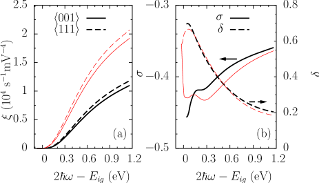
Figure 4: (Color online) (a) Spectra of total carrier injection rates $\xi$ at 4 K and 300 K for $\sigma^{-}$ light propagating along the $\langle 001\rangle$ and $\langle 111\rangle$ directions. (b) Anisotropy $\sigma$ and linear-circular dichroism $\delta$ at 4 K (thick black curves) and 300 K (thin red curves).

We plot photon energy dependence of the total carrier injection coefficients for $\langle 001\rangle$ and $\langle 111\rangle$ light at 4 K and 300 K in Fig. 4 (a). As we found earlier in a preliminary studyAppl.Phys.Lett._98_131101_2011_Cheng , the injection coefficients increase rapidly with increasing temperature. The injection for $\langle 111\rangle$ light is larger than that for $\langle 001\rangle$ light, demonstrating the anisotropy of the injection on light propagating direction. In agreement with Hutchings and Wherrett’s notationPhys.Rev.B_49_2418_1994_Hutchings for direct gap two-photon injection, this anisotropy can be characterized by two parameters, the anisotropy $\sigma$ and the linear-circular dichroism $\delta$, which are given as

$$\sigma = \frac{\xi^{xxxx}-2\xi^{xyxy}-\xi^{xxyy}}{\xi^{xxxx}}\ ,$$

$$\delta = \frac{\xi^{xxxx}-2\xi^{xyxy}+\xi^{xxyy}}{2\xi^{xxxx}}\ .$$ (18)

In the isotropic limit, $\sigma=0$ and $\delta=\xi^{xxyy}/\xi^{xxxx}$Opt.Mater._3_53_1994_Hutchings . We plot $\sigma$ and $\delta$ in Fig. 4 (b). Note that the anisotropy shows a much stronger temperature dependence than the linear-circular dichroism. In contrast to $\sigma$ in direct gap two-photon injection, which clearly shows the onset of the transition from the spin split-off band to the conduction band by the presence of a cusp, it is hard to identity the contribution from spin split-off band in indirect gap injection. This is because the energy dependence at the onset of indirect absorption is $\propto(\hbar\omega-E_{ig})^{2}$, given by the $a-a$ process, instead of $\propto(\hbar\omega-E_{g})^{1/2}$ for direct absorption.

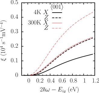
Figure 5: (Color online) Spectra of carrier injection rates $\xi_{I}^{\langle 001\rangle}$ in the $I=Z$ and $X$ valley at 4 (thick black curves) and 300 K (thin red curves).

Now we turn to the carrier injection into each valley. For $\langle 111\rangle$ light, all valleys are equivalent, and the injection coefficient in each valley is $1/6$ of the total. There is no valley anisotropy in this case. For $\langle 001\rangle$ light, the valleys can be divided into two sets: $\{Z,\bar{Z}\}$ and $\{X,\bar{X},Y,\bar{Y}\}$, and the injection is the same for all valleys within each set. We plot the spectra of injection rates $\xi_{I}^{\langle 001\rangle}$ in the $I=Z$ and $X$ valleys at 4 K and 300 K in Fig. 5. The spectrum in each valley has a shape similar to the total, and the injection in the $Z$ valley is larger than that in the $X$ valley. The valley anisotropy arises because of the anisotropic effective electron mass in the conduction bands, which leads to different matrix elements appearing in (4) for the different Cartesian components of velocity. For the $Z$ valley, the effective mass along the $z$ direction is heavier than that along the $x/y$ directionslandolt_Si , which results in a smaller $z$ component of the interband velocity matrix elementseffectivemass . From Table 4, we find that the $z$-components of the electron and hole velocity only appears in the injection rates in the $X/Y$ valleys, and results in their smaller injection rates.

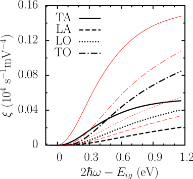
Figure 6: (Color online) Phonon resolved spectra of carrier injection rates $\xi_{X;\tau}^{\langle 111\rangle}$ at 4 K (thick black curves) and 300 K (thin red curves).

Figure 6 gives the phonon-resolved spectra in the $X$ valley for $\langle 111\rangle$ light. Similar to our previous resultsAppl.Phys.Lett._98_131101_2011_Cheng , we find here that the LA phonon-assisted process gives the smallest contribution, while the TA and TO phonon-assisted processes dominate: At low temperature, the TA phonon-assisted process dominates at low photon energy, and the TO phonon-assisted process dominates at high photon energy; with temperature increasing, the TA phonon-assisted process becomes more and more important due to the small TA phonon energy, and dominates for photon energy less than $E_{ig}$ at 300 K. The phonon-resolved injection rates in each valley for $\langle 001\rangle$ light show similar behavior.

II.2.4 Spin injection under $\sigma^{-}$ light propagating along $\langle 001\rangle$ and $\langle 111\rangle$

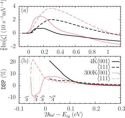
Figure 7: (Color online) Spectra of (a) spin injection rates $\zeta^{\langle\hat{\bm{k}}\rangle}$ and (b) $\text{DSP}^{\langle\hat{\bm{k}}\rangle}$ at 4 K (black curves) and 300 K (red curves). (Solid curves) $\bm{E}\parallel\langle 001\rangle$, (dashed curves) $\bm{E}\parallel\langle 111\rangle$. The spin polarization direction is parallel to $\bm{E}$. The labeled energies are $2\hbar\omega_{1-3}-E_{ig}=-\Omega_{\text{TO}}^{0}$, $-\Omega_{\text{LA}}$, $-\Omega_{\text{TA}}$, and $2\hbar\omega_{3}^{\prime}-E_{ig}=\Omega_{\text{TA}}$.

In Fig. 7 we show the spectra of the spin injection rates $\zeta^{\langle\hat{\bm{k}}\rangle}$ and the $\text{DSP}^{f}$ for $\sigma^{-}$ light propagating along $\langle 001\rangle$ and $\langle 111\rangle$ directions at 4 K and 300 K. The total spin polarizations are all parallel to light propagation direction. When photon energy is higher than the injection edge, which is $E_{ig}+\hbar\Omega_{\text{TA}}^{0}$ at 4 K or $E_{ig}-\hbar\Omega_{\text{TO}}^{0}$ at 300 K, the spin injection rates first increase with photon energy from zero to maximum values, then decrease, and then change direction at high photon energies. This is different than the behavior of indirect one-photon spin injection, in which the spin injection rates always increase with photon energy. The difference can be attributed to the complicated transition amplitude $W$ in Eq. (4). The fine structure of the injection rates around the band edge are clearly shown by the DSP spectra in Fig. 7(b). The DSP depends strongly on the laser propagation direction and the temperature. For $\langle 001\rangle$ light, the maximum DSP can reach about $20\%$ at 4 K and $-10\%$ at 300 K; for $\langle 111\rangle$ light, the maximum DSP is only $6\%$ at 4 K but $20\%$ at 300 K. Around the injection edges, the DSP show more detailed structures at 300 K than 4 K. In Fig. 7(b), we label the injection edge for phonon branches by dotted vertical lines: $\hbar\omega_{1}$, $\hbar\omega_{2}$, and $\hbar\omega_{3}$ for the TO, LO, and TA phonon absorption process, respectively; $\hbar\omega_{3}^{\prime}$ identifies the TA phonon emission process. As in the corresponding results for indirect one-photon spin injection, the fine structures arising here come from the contributions of different phonon branches.

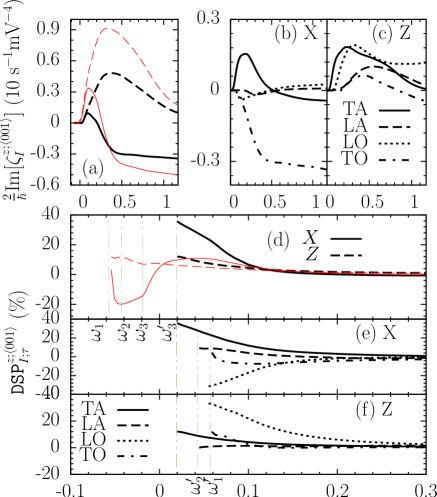
Figure 8: (Color online) Spectra of (a) spin injection rates $\zeta_{I}^{\langle 001\rangle}$ in the $I=X$ valley (solid curves) and the $I=Z$ valley (dashed curve) at 4 K (thick black curves) and 300 K (thin red curves), (b)-(c) phonon branch resolved spin injection rates in the $X$ and $Z$ valleys at 4 K, and (d-f) The corresponding DSP of (a-c).The labeled energies are $2\hbar\omega_{1-2}^{\prime}=\Omega_{\text{TO}}^{0}$ and $\Omega_{\text{LA}}^{0}$, respectively.

To better understand these fine structures, we plot the spin injection in each valley and the contribution from each phonon branches for $\langle 001\rangle$ light in Fig. 8. Figure 8(a) gives the spin injection rates in the $X$ and $Z$ valleys at 4 K and 300 K, in which the valley anisotropy is prominent. Again, due to the anisotropy in electron velocity, the injection rate in the $Z$ valley is much larger than that in the $X$ valley. Figure 8 (d) gives the detailed structure of DSP around the band edge. The maximum DSP is about $36\%$ at 4 K and $-20\%$ at 300 K in the $X$ valley, and about $10\%$ in the $Z$ valley for both temperatures. However, the spin injection rates are very close in these two valleys near the injection edge in Fig. 7(a), so the difference between these maximum values can only come from the difference of the carrier injection rates, which are much smaller in the $X$ valley than that in the $Z$ valley (see Fig. 5).

The phonon-resolved spin injection rates in the $X$ and $Z$ valleys are plotted in Figs. 8 (b-c) at 4 K . In the $X$ valley, the TA phonon branch dominates at low photon energy, and the TO phonon branch dominates at high photon energy. In the $Z$ valley, the TA and LO phonon branches have similar contributions and dominate at low photon energy. Near the band edge, the spins injected from the TO and TA phonon-assisted processes have opposite spin polarization direction in the $X$ valley, but same in the $Z$ valley. Figures 8 (e-f) give the corresponding DSP. Almost all processes contribute nonzero DSP. In the $Z$ valley, the spin injection rates are given by $\text{Im}[\zeta_{Z;\tau}^{zxyxx}]$ as shown in Table 4. At the band edges, the carrier and spin injection amplitude of the LA and LO phonon-assisted processes are all zero, which means these $a-a$ processes inject no carriers. As one moves away from the band edges, carriers and spins can be injected by $a-f$ and $f-f$ processes, which results in a nonzero DSP. In the $X$ valley, the spin injection rates are given by $\text{Im}[\zeta_{Z;\tau}^{xzzyz}+\zeta_{Z;\tau}^{xyzyy}]$. From the results in Table 3, we see that the LA phonon-assisted process gives zero spin injection amplitude at band edge, but its DSP is not zero because the $a-f$ and $f-f$ processes dominate over the $a-a$ process. Similar results also exist in two-photon direct injectionPhys.Rev.B_71_035209_2005_Bhat .

In Figs. 8 (e-f), we plot only the DSP for the phonon emission processes, the corresponding injection edges are given by $\hbar\omega_{i}^{\prime}$. From the calculation of the indirect one-photon injection, we know that the DSP induced by the phonon absorption process and the phonon emission process have a similar shape, but the injection edge shifts from $\hbar\omega_{i}^{\prime}$ to $\hbar\omega_{i}$. At 4 K, the injection edge is dominated by the TA phonon emission process (which begins at $\hbar\omega_{3}^{\prime}$), and it is dominated by the TO/LO phonon absorption process (begins at $\hbar\omega_{1}$) at 300 K, then follows by the LA phonon absorption process at $\hbar\omega_{2}$ and the TA phonon at $\hbar\omega_{3}$. Therefore, the co-action of the TO and LO phonon absorption processes gives the negative DSP, and results in the sharp increase between the photon energies $\hbar\omega_{1}$ and $\hbar\omega_{2}$ in Fig. 8 (c), then the LA/TA phonon absorption processes give positive DSP, so the total DSP decreases sharply after $\hbar\omega_{2}$.

Figure 9 gives the details of the spin injection for the $\sigma^{-}$ light propagating along $\langle 111\rangle$ direction. The analysis is similar to the $\langle 001\rangle$ case.

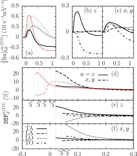
Figure 9: (Color online) Spectra of (a) spin injection rates $\zeta_{Z}^{a;\langle 111\rangle}$ and (d) $\text{DSP}_{Z}^{a;\langle 111\rangle}$ for the $a=z$ (solid curves) and $x,y$ (the dashed curves) spin components at 4 K (thick black curves) and 300 K (thin red curves). Phonon resolved (b-c) spin injection rates $\zeta_{Z;\tau}^{a;\langle 111\rangle}$ and (e-f) $\text{DSP}_{Z;\tau}^{a;\langle 111\rangle}$ for the $z$ (black thick curves) and $x,y$ (blue thin curves) spin components at 4 K.

III Two-color charge and spin current injection

Now we study the motions of optically injected carriers and spins. While a single color light source can inject net current into a particular valleyJETPLett._81_231_2005_Tarasenko ; Phys.Rev.B_83_121312_2011_Karch , due to the $O_{h}$ symmetry there is no net charge or spin current injection from either either one-photon or two-photon absorption of a single color light source. We calculate $1+2$ injection effects here, and only consider the total charge and spin current induced. For a two-color optical field ${\bm{E}}(t)={\bm{E}}_{\omega}e^{-i\omega t}+{\bm{E}}_{2\omega}e^{-i2\omega t}+c.c$, the carrier density injection rate is

$$\dot{n} = \xi^{ab}E_{2\omega}^{a}(E_{2\omega}^{b})^{\ast}+\xi^{abcd}E_{\omega}^{a}E_{\omega}^{b}(E_{\omega}^{c}E_{\omega}^{d})^{\ast}\ ,$$ (19)

where $\xi_{i}^{ab}$ are one-photon indirect injection coefficientsPhys.Rev.B_83_165211_2011_Cheng and $\xi^{abcd}$ are the two-photon injection coefficients studied in the previous sections. The interference between $\omega$ and $2\omega$ beams injects charge and spin currents with injection rates

$$\dot{J}^{d}_{e(h)} = \eta_{e(h)}^{dabc}E^{a}_{2\omega}(E^{b}_{\omega}E^{c}_{\omega})^{\ast}+c.c.\ ,$$

$$\dot{K}^{fd}_{e(h)} = \mu_{e(h)}^{dfabc}E^{a}_{2\omega}(E^{b}_{\omega}E^{c}_{\omega})^{\ast}+c.c.\ .$$ (20)

The injection coefficients $\eta_{e(h)}^{dabc}$ and $\mu^{dfabc}_{e(h)}$ are written in the form ${\cal B}^{abc}=\sum_{\lambda\pm}{\cal B}^{abc}_{\lambda\pm}$ with

$${\cal B}^{abc}_{\lambda\pm} = \frac{2\pi}{\hbar}\sum_{c\bm{k}_{c},v\bm{k}_{v}}\delta(\varepsilon_{c\bm{k}_{c}}-\varepsilon_{v\bm{k}_{v}}\pm\hbar\Omega_{(\bm{k}_{c}-\bm{k}_{v})\lambda}-2\hbar\omega)$$ (21)

$$\times N_{(\bm{k}_{c}-\bm{k}_{v})\lambda\pm}{\cal B}^{abc}_{c\bm{k}_{c}v\bm{k}_{v}\lambda}\ ,$$

$${\cal B}^{abc}_{c\bm{k}_{c}v\bm{k}_{v}\lambda} = i\sum_{\sigma_{c}\sigma_{c}^{\prime};\sigma_{v}\sigma_{v}^{\prime}}\langle\bar{c}^{\prime}\bm{k}_{c}|\langle\bar{v}^{\prime}\bm{k}_{v}|\hat{\cal B}|\bar{v}\bm{k}_{v}\rangle|\bar{c}\bm{k}_{c}\rangle$$ (22)

$$\times T^{a}_{\bar{c}\bm{k}_{c}\bar{v}\bm{k}_{v}\lambda}(2\omega)[W^{bc}_{\bar{c}^{\prime}\bm{k}_{c}\bar{v}^{\prime}\bm{k}_{v}\lambda}(\omega)]^{\ast}\ .$$

Here $T^{a}_{\bar{c}\bm{k}_{c}\bar{v}\bm{k}_{v}\lambda}$ is the one-photon indirect optical transition amplitude Phys.Rev.B_83_165211_2011_Cheng . By taking $\hat{\cal B}$ as $\hat{J}_{e}^{d}=-e\hat{v}_{e}^{d}$, $\hat{J}_{h}^{d}=e\hat{v}_{h}^{d}$, $\hat{K}_{e}^{fd}=-\frac{e}{\hbar}(\hat{v_{e}}^{d}\hat{S}_{e}^{f}+\hat{S}_{e}^{f}\hat{v}_{e}^{d})$, and $\hat{K}_{h}^{fd}=\frac{e}{\hbar}(\hat{v_{h}}^{d}\hat{S}_{h}^{f}+\hat{S}_{h}^{f}\hat{v}_{h}^{d})$, we obtain the injection rates for electron and hole charge and spin currents, with $\eta^{dabc}=\eta^{dacb}$ and $\mu^{dfabc}=\mu^{dfacb}$. For diamond structure crystals, the nonzero components are

$$\eta^{xxxx} \ ,$$

$$\eta^{xxyy} = \eta^{xxzz}\ ,$$

$$\eta^{xyxy} = \eta^{xzxz}\ .$$ (23)

and

$$\mu^{zxxxy} = -\mu^{zyyyx}\ ,$$

$$\mu^{zxyxx} = -\mu^{zyxyy}\ ,$$

$$\mu^{zxyyy} = -\mu^{zyxxx}\ ,$$

$$\mu^{zxyzz} = -\mu^{zyxzz}\ ,$$

$$\mu^{zxzyz} = -\mu^{zyzxz}\ ,$$

$$\mu^{zzxyz} = -\mu^{zzyxz}\ .$$ (24)

All other nonzero components can be obtained by cyclic permutations of the Cartesian indices. The phonon-resolved tensors $\eta^{dabc}_{e(h);\lambda\pm}$ and $\mu^{dfabc}_{e(h);\lambda\pm}$ share the same symmetry properties as the total injection tensor $\eta^{dabc}_{e(h)}$ and $\mu^{dfabc}_{e(h)}$, respectively. Using time-reversal symmetry, in the independent particle approximation we adopt here all $\eta^{dabc}$ are pure imaginary numbers, and all $\mu^{dfabc}$ are real numbers. We show the calculated spectra of each component of the charge current in Fig. 10, and of the spin current in Fig. 11. The current injection coefficients $\eta_{e(h)}^{dabc}$ and $\mu_{e(h)}^{dfabc}$ have the same symmetry properties as that of the two-color direct current injection across the direct gap of germanium Phys.Rev.B_81_155215_2010_Rioux .

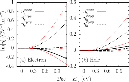
Figure 10: (Color online) Spectra of $\text{Im}[\eta^{fabc}]$ for electron (a) and hole (b) at 4 K (thick black curves) and 300 K (thin red curves).

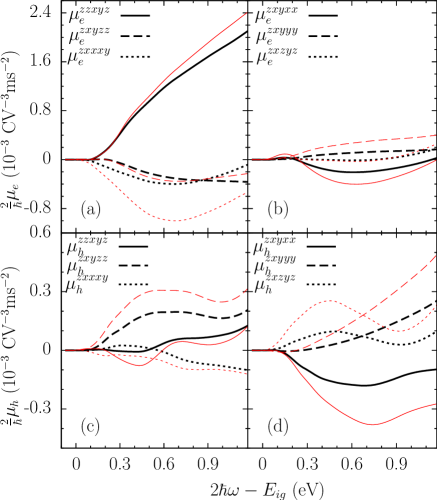
Figure 11: (Color online) Spectra of $\mu_{e}^{dfabc}$ for electron (a) and hole (b) at 4 K (thick black curves) and 300 K (thin red curves)

From the calculation, both the charge and the spin currents for injected electrons are larger than that for injected holes. One contributing factor is that the electron moves faster than the hole due to the smaller effective mass. But for the spin current, another factor is that the average spin expectation value over the HH and LH band is smaller than that in the conduction bands.

We consider the indirect current injection coefficients under the two-color laser beams propagating along the $z$ direction with the electric field components taken as $\bm{E}_{\omega}=E_{\omega}e^{i\phi_{\omega}}\hat{\bm{e}}_{\omega}$ and $\bm{E}_{2\omega}=E_{2\omega}e^{i\phi_{2\omega}}\hat{\bm{e}}_{2\omega}$. Here $E_{\omega}$ and $E_{2\omega}$ are real and positive field amplitudes, $\hat{\bm{e}}_{\omega}$ and $\hat{\bm{e}}_{2\omega}$ are polarization vectors, and $\phi_{\omega}$ and $\phi_{2\omega}$ are their phases, and $\Delta\phi\equiv 2\phi_{\omega}-\phi_{2\omega}$ is the relative-phase parameter that is used to control the current. In the following, we give the current injection for different configurations of the laser beams.

III.1 Co-circularly polarized beams

For two circularly polarized beams propagating along the $z$ direction, the electric fields are $\hat{\bm{e}}_{2\omega}=\hat{\bm{\sigma}}^{s_{2}}$ and $\hat{\bm{e}}_{\omega}=\hat{\bm{\sigma}}^{s_{1}}$ with $s_{i}=\pm$ identifying for the handedness and ${\bm{\sigma}}^{s}=(\hat{\bm{x}}+is\hat{\bm{y}})/\sqrt{2}$. The indirect gap current injection coefficients are

$$\dot{\bm{J}}_{e(h)} = s_{1}\text{Im}[\eta_{e(h)}^{xxxx}-\eta_{e(h)}^{xyyx}+2s_{1}s_{2}\eta_{e(h)}^{xxyy}]\frac{E^{2}_{\omega}E_{2\omega}}{\sqrt{2}}\hat{\bm{m}}_{s_{1}}\ ,$$

$$\dot{K}_{e(h)}^{ab} = [\mu_{e(h)}^{zxyyy}-\mu_{e(h)}^{zxyzz}+s_{1}s_{2}\mu_{e(h)}^{zxzyz}]\frac{E^{2}_{\omega}E_{2\omega}}{\sqrt{2}}\hat{\bm{m}}_{s_{1}}^{a}\hat{\bm{z}}^{b}$$ (25)

$$-[\mu_{e(h)}^{zxyyy}-\mu_{e(h)}^{zxyxx}+s_{1}s_{2}\mu_{e(h)}^{zxxxy}]\frac{E^{2}_{\omega}E_{2\omega}}{\sqrt{2}}\hat{\bm{z}}^{a}\hat{\bm{m}}_{s_{1}}^{b}$$

with $\bm{m}_{s_{1}}=s_{1}\hat{\bm{x}}\sin\Delta\phi+\hat{\bm{y}}\cos\Delta\phi$. Both the direction of the charge and spin currents and the polarization of the spin current can be controlled by the relative-phase parameter $\Delta\phi$ and the light polarization $s_{i}$. The charge current flows only in the $x-y$ plane, and the calculated $\eta_{e(h)}^{xxyy}$ is negligible. For the opposite circularly-polarized beams, the $x$ component of the charge current is kept unchanged, but the $y$ component reverses. The spin current flows in the $x-y$ plane with spin polarization along $x$-axis, or flows along $z$-direction with spin polarization along $x/y$ direction.

III.2 Cross-linearly polarized beams

For two $z$ propagating cross-linearly polarized beams, $\bm{E}_{\omega}$ along the $\hat{\bm{x}}$ direction and $\bm{E}_{2\omega}$ along the $\hat{\bm{y}}$ direction, the injection current rates are given as

$$\dot{\bm{J}}_{e(h)} = 2\text{Im}[\eta_{e(h)}^{xxyy}]E^{2}_{\omega}E_{2\omega}\hat{\bm{y}}\sin\Delta\phi\ ,$$ (26)

$$\dot{K}_{e(h)}^{ab} = 2(\mu_{e(h)}^{zxyxx}\hat{\bm{z}}^{a}\hat{\bm{x}}^{b}-\mu_{e(h)}^{zxyzz}\hat{\bm{x}}^{a}\hat{\bm{z}}^{b})E^{2}_{\omega}E_{2\omega}\cos\Delta\phi\ .$$

In this scenario, the charge current and the spin current are injected with $\pi/2$ phase difference. Therefore, by tuning the relative-phase parameter $\Delta\phi$, a pure charge current or pure spin current can be injected. The charge current flows along the second harmonic polarization axis, and its amplitude is determined by $\eta^{xxyy}$, which is zero under the parabolic band approximation. In our full band structure calculation, it is nonzero due to the band warping, but very small compared to other tensor components. The spin current has two components, one involving flow along the $x$ direction with the $z$ spin polarization, and the other involving flow along the $z$ direction with the $x$ spin polarization.

III.3 Co-linearly polarized beams

For two $z$ propagating beams, both polarized along the $x$ direction, the injection current rates are given as

$$\dot{\bm{J}}_{e(h)} = 2\text{Im}[\eta_{e(h)}^{xxxx}]E^{2}_{\omega}E_{2\omega}\hat{\bm{x}}\sin\Delta\phi\ ,$$

$$\dot{K}_{e(h)}^{ab} = 2\mu_{e(h)}^{zxyyy}(\hat{\bm{y}}^{a}\hat{\bm{z}}^{b}-\hat{\bm{z}}^{a}\hat{\bm{y}}^{b})E^{2}_{\omega}E_{2\omega}\cos\Delta\phi\ .$$ (27)

This scenario also gives the phase difference between the charge current and the spin current as $\pi/2$, so as for cross-linearly polarized beams pure charge current injection or the pure spin current injection can also be realized by choosing a suitable relative-phase parameter $\Delta\phi$. Our results give the relative-phase parameter dependence of the injected current as $\sin\Delta\phi$, which is in good agreement with the experimental resultsNaturePhys._3_632_2007_Costa around zero probe delay. To understand the indirect current injection better, we compare the indirect current injection with the direct one. Because of the lack of the direct gap injection in silicon in the literature, our results are compared with the direct current injection in bulk germaniumPhys.Rev.B_81_155215_2010_Rioux . For the charge currents injected across the indirect gap in silicon, the electron and hole currents have opposite directions at high photon energies, but they can be the same at low energies; for charge currents injected across the direct gap in germanium, they always have the same directions. For the spin current, the injected spin current is not so small compared to other components, especially at 300 K, while they are ignorable small in the direct gap current injection in germanium because of the complete lack of the helicity of the incident light.

In this configuration, a good characterization of the charge current is the swarm velocity, which is defined as the average velocity per injected carriers forming this current, $v_{s}^{x}=\dot{J}^{x}/e_{s}\dot{n}$, with $\dot{n}$ taken from Eq. (19). Here $e_{s}=-e$ is used for electrons and $e_{s}=e$ for holes. When $\Delta\phi$ is a multiple of $\pi/2$ and the indirect one-photon charge injection rate equals the indirect two-photon charge injection rate, the maximum swarm velocity is

$$v_{s,\text{max}}^{x}(\omega)=\frac{\text{Im}[\eta_{s}^{xxxx}(\omega)]}{e_{s}\sqrt{\xi_{s}^{xx}(2\omega)\xi_{s}^{xxxx}(\omega)}}\ .$$ (28)

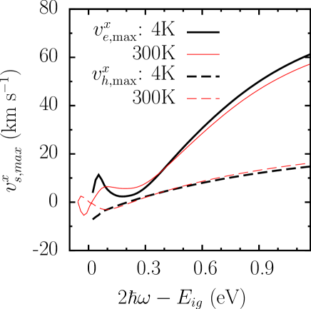
Figure 12: (Color online) Maximal swarm velocity $v^{x}_{s,max}$ for the injected electrons (solid curves) and holes (dashed curves) at 4 K (thick black curves) and 300 K (thin red curves).

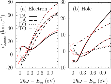
Figure 13: (Color online) Phonon-resolved Maximal swarm velocity for the injected (a) electrons and (b) holes at 4 K (thick black curves) and 300 K (thin red curves).

We show the maximum swarm velocity in Fig. 12 for the injected electrons and holes at 4 K and 300 K. The behavior of the swarm velocity can be divided into two regions: (i) for photon energies in $2\hbar\omega-E_{ig}\gtrapprox 0.25$ eV, the maximum swarm velocities are along the $x$ direction for injected electrons and holes, and both magnitudes increase with increasing photon energy. Compared to the maximum swarm velocities in bulk germanium, which is in the order of $10^{3}$ km/s, the velocity here is about one order of magnitude smaller due to the larger conduction band effective mass in silicon. (ii) for photon energies in $2\hbar\omega-E_{ig}<0.2$ eV, the swarm velocities show fine structures. In particular, all currents experience directional changes except the electron swarm velocity at 4 K. Analogous to indirect one- and two-photon charge and spin injection, these fine structures are induced by the different phonon branches, which are clearly shown in the phonon-resolved maximal swarm velocity in Fig. 13. At 300 K, the injection edge is given by the TO/LO phonon absorption processes, both of which give negative velocities for injected electrons and positive velocities for holes around the injection edge. At 4 K, the injection edge is given by the TA phonon emission process, which direction is opposite to the band edge current at 300 K. Therefore, the sign change of the injected current is induced by the contributions from different phonon branches. At high photon energies, the injected velocities are almost independent of the temperature. This is similar to the temperature dependence of the DSP of the one-photon indirect injectionPhys.Rev.B_83_165211_2011_Cheng : The only temperature dependence in the injection rates lies in the phonon number, which is the same for the denominator and numerator in Eq. (28) for a given phonon branch. For high photon energies, an average phonon number can be used as a good approximation, and the swarm velocities, given by the ratio in Eq. (28), are almost temperature independent.

IV Conclusion

In conclusion, we have performed a full band structure calculation of two-photon indirect carrier and spin injection, and two-color indirect current injection, in bulk silicon. We presented the spectral dependence for all components of the response tensors at 4 K and 300 K, with which the injection under any laser beams can be extracted. All injection rates increase with increasing temperature due to strong electron phonon interaction at high temperature. We discussed in detail the injection under different polarized light beams.

For two-photon indirect optical carrier and spin injections, we considered the injection under $\sigma^{-}$ light propagating along $\langle 001\rangle$ and $\langle 111\rangle$ directions. For $\langle 001\rangle$ light, the injection rates in the $X$ and $Y$ valleys are the same, but different from that in the $Z$ valley; for the $\langle 111\rangle$ light, the injections into all valleys are equivalent. For carrier injection, injections for these two light propagation axes differ slightly. The calculated injection anisotropy and the linear-circular dichroism characterize the nonparabolic band effect in the full band structure calculation. For the $\langle 001\rangle$ light, the injection in the $Z$ valley are much larger than that in the $X$/$Y$ valleys, and give the valley anisotropy, which is induced by the velocity anisotropy in the conduction band. At 4 K, the TA phonon-assisted process dominates at low photon energies, and the TO phonon-assisted process dominates at high photon energies. At 300 K, the TA phonon-assisted process dominates for all photon energies.

For two-photon indirect gap spin injection, the total injected spins orient parallel to the light propagation direction for the two directions considered. The spin injection rates increase from the injection edge to a maximum value with the photon energy increasing, and then decrease. The DSP strongly depends on the temperature around the injection edge. For the $\langle 001\rangle$ light, the injected spins in each valley are still along the $z$ direction, but the spin injection rates in the $X$ and $Z$ valleys are different. The maximum DSP of total spins is $20\%$ at 4 K and $-10\%$ at 300 K; the DSP can reach about $40\%$ at 4 K and $-20\%$ at 300 K in the $X$ valley, and both become $10\%$ in the $Z$ valleys. For $\langle 111\rangle$ light, the spins in each valley orient to a direction different from the light propagating direction. In the $Z$ valley, the $x$ and $y$ (transverse) components have the same injection rates, which are different from the $z$ (longitudinal) component. The maximum DSPs of the total spins are $6\%$ at 4 K and $20\%$ at 300 K, while the one of the $z$ component spin in the $Z$ valley is about $5\%$ at 4 K and $20\%$ at 300 K, and becomes $25\%$ and $-8\%$ for the $x$ or $y$ components. All these features are induced by the interplay of different phonon branch-assisted processes.

For light propagating along the $\langle 001\rangle$ direction, the injected carriers or spins break the symmetry between the $X$ and $Z$ valleys. Such a valley anisotropy of injected carriers could be probed experimentally, for example, in a pump-probe scenario where the probe beam propagates either parallel or perpendicular to the pump beam.

For the coherent control, we calculated two-color indirect charge and spin current injection under three different polarization configuration of the two-color beams propagating along the $z$ direction. For the co-circularly polarized beams, the direction of the injected charge current is in the $x-y$ plane; the spin current flows in the $x-y$ plane with a $z$ oriented spin polarization, or flows along the $z$ direction with the spin orientation in the $x-y$ plane; the current direction or the spin polarization in the $x-y$ plane can be controlled by a relative-phase parameter. For the co-linearly polarized beams and the cross-linearly polarized beams, the directions of the charge current, the spin current, and the spin polarization are orthogonal to each other. In these two cases, a pure spin current or a pure charge current can be obtained by choosing a suitable relative-phase parameter. We calculated the maximum swarm velocity for charge current as a function of photon energy, and found that the maximum swarm velocities undergo a sign change near the band edge, which is induced by the contributions from different phonon branches.

Appendix A Dependence of the injection rates on the light propagating direction

For a circularly polarized laser pulse propagating along direction $\hat{\bm{n}}_{1}$, the electric field can be expressed as

$$\bm{E}_{\omega}=\frac{E_{0}}{\sqrt{2}}(\hat{\bm{n}}_{2}+is\hat{\bm{n}}_{3})$$ (29)

with

$$\hat{\bm{n}}_{1}=\begin{pmatrix}\sin\theta\cos\phi\\ \sin\theta\sin\phi\\ \cos\theta\end{pmatrix}\,,\quad\hat{\bm{n}}_{2}=\begin{pmatrix}\sin\phi\\ -\cos\phi\\ 0\end{pmatrix}\,,\quad\hat{\bm{n}}_{3}=\hat{\bm{n}}_{1}\times\hat{\bm{n}}_{2}\,,$$ (30)

here $s=\pm 1$ identifies the helicity. In the $Z$ valley the carrier injection rates can be written as

$$\dot{n}_{Z} = E_{0}^{4}\Big{[}\frac{1}{8}(1+\cos^{2}\theta)^{2}(\xi_{Z}^{xxxx}-\xi_{Z}^{xxyy}+2\xi_{Z}^{xyxy})$$ (31)

$$+ \frac{1}{8}(\sin^{2}\theta\cos 2\phi)^{2}(\xi_{Z}^{xxxx}-\xi_{Z}^{xxyy}-2\xi_{Z}^{xyxy})$$

$$+ \frac{1}{4}\sin^{4}\theta(\xi_{Z}^{zzzz}+\xi_{Z}^{xxyy}-2\xi_{Z}^{zzxx})$$

$$+ \sin^{2}\theta(1+\cos^{2}\theta)\xi_{Z}^{xzxz}\Big{]}\,,$$

and the spin injection rates as

$$\dot{\bm{S}}_{Z} = E_{0}^{4}s\Big{\{}-(\cos^{2}\theta+1)\cos\theta\text{Im}[\zeta_{Z}^{zxyxx}]\hat{\bm{z}}$$ (32)

$$- 2\sin^{2}\theta\cos\theta\text{Im}[\zeta_{Z}^{zyzxz}]\hat{\bm{z}}-\sin^{3}\theta\text{Im}[\zeta_{Z}^{xzzyz}]\hat{\bm{n}}_{3}^{\prime}$$

$$+ \frac{1}{4}\bm{g}_{1}(\theta,\phi)\sin\theta\text{Im}[-\zeta_{Z}^{xyzyy}+\zeta_{Z}^{xyzxx}+2\zeta_{Z}^{xxzxy}]$$

$$- \sin^{2}\theta\sin\theta\text{Im}[\zeta_{Z}^{xyzxx}]\hat{\bm{n}}_{3}^{\prime}$$

$$- (3+\cos 2\theta)\sin\theta\text{Im}[\zeta_{Z}^{xxzxy}]\hat{\bm{n}}_{3}^{\prime}\Big{\}}$$

with $\hat{\bm{n}}_{3}^{\prime}=\hat{\bm{z}}\times\hat{\bm{n}}_{2}$ and

$$\bm{g}_{1}(\theta,\phi)=(\sin^{2}\theta\sin 4\phi)\hat{\bm{n}}_{2}+[4+\sin^{2}\theta(\cos 4\phi-1)]\hat{\bm{n}}_{3}^{\prime}\,.$$ (33)

For an arbitary propagating direction $(\theta,\phi)$, the direction of the spin polarization is not always along $\hat{\bm{n}}_{1}$. In this case, we define DSP as the ratio of the magnitude of the spin injection rate and the carrier injection rate $P_{Z}=|\dot{\bm{S}}_{Z}|/(\dot{n}_{Z}\hbar/2)$. We plot in Fig. 14 the $(\theta,\phi)$-dependence of the $P_{z}$ at the edge of the each phonon emission process in the $Z$ valley, which shows strong anisotropy of the light propagating direction. The maximum $P_{z}$ can reach 45% at $(\theta,\phi)\approx(\pi/2,0.2\pi)$ for the TA phonon emission process, 20% at $\approx(\pi/2,0.1\pi)$ for LA phonon, 45% at $\theta\approx\pi/4$ for LO phonon, and 13% at $\theta\approx 0.2\pi$ for TO phonon.

Figure 14: (Color online) Light propagating dependence of the $P_{z}$ at the edge of the each phonon emission process in the $Z$ valley. (a) TA phonon, (b) LA phonon, (c) LO phonon, (d) TO phonon.

The total carrier injection rates are

$$\dot{n} = E_{0}^{4}\xi^{xxxx}\Big{[}1-\delta-\frac{\sigma}{2}\sin^{2}\theta(\sin^{2}\phi\cos^{2}\phi\sin^{2}\theta+\cos^{2}\theta)\Big{]}\,,$$

with $\delta$ and $\sigma$ defined in Eqs. (18). The total spin injection rates are

$$\dot{\bm{S}} = E_{0}^{4}s\Big{\{}-2\text{Im}[\zeta^{zxyxx}]\hat{\bm{n}}_{1}$$ (35)

$$+\frac{1}{4}\sin\theta\bm{g}_{2}(\theta,\phi)\text{Im}[\zeta^{zxyxx}-2\zeta^{xxzxy}]\Big{\}}\,,$$

with

$$\bm{g}_{2}(\theta,\phi) = \sin\theta(1+7\cos^{2}\theta-\sin^{2}\theta\cos 4\phi)\hat{\bm{n}}_{1}$$ (36)

$$- (\sin^{2}\theta\sin 4\phi)\hat{\bm{n}}_{2}$$

$$- \cos\theta(3-7\cos^{2}\theta+\sin^{2}\theta\cos 4\phi)\hat{\bm{n}}_{3}\,.$$

From above expressions, the two-photon carrier and spin injection rates show strong anisotropy for the light propagating direction. For the spin injection, the direction of the injected spin polarization usually differs from the light propagating direction, but it reverses as the light helicity changes.

For the linear polarized laser pulse, we also found that the total carrier injection rates strongly depend on the polarization direction. For the electric field

$$\bm{E}_{\omega}=E_{0}(\hat{\bm{n}}_{2}\sin\alpha+\hat{\bm{n}}_{3}\cos\alpha)\,,$$ (37)

with $\alpha$ for the polarization direction, the total carrier injection rates are given by

$$\dot{n} = E_{0}^{4}\xi^{xxxx}\{1-[1-f(\theta,\phi,\beta)]\sigma\}\,,$$ (38)

with

$$f(\theta,\phi,\beta) = (\cos\phi\sin\alpha-\cos\theta\sin\phi\cos\alpha)^{4}$$ (39)

$$+ (\sin\phi\sin\alpha+\cos\theta\cos\phi\cos\alpha)^{4}$$

$$+ \sin^{4}\theta\cos^{4}\alpha\,.$$