Bifurcations in Boolean Networks

Abstract

This paper characterizes the attractor structure of synchronous and asynchronous Boolean networks induced by bi-threshold functions. Bi-threshold functions are generalizations of standard threshold functions and have separate threshold values for the transitions $0\to 1$ (up-threshold) and $1\to 0$ (down-threshold). We show that synchronous bi-threshold systems may, just like standard threshold systems, only have fixed points and $2$-cycles as attractors. Asynchronous bi-threshold systems (fixed permutation update sequence), on the other hand, undergo a bifurcation. When the difference $\Delta$ of the down- and up-threshold is less than $2$ they only have fixed points as limit sets. However, for $\Delta\geq 2$ they may have long periodic orbits. The limiting case of $\Delta=2$ is identified using a potential function argument. Finally, we present a series of results on the dynamics of bi-threshold systems for families of graphs.

1 Introduction

A standard Boolean threshold function $\text{\emph{t}}_{k,m}\colon\{0,1\}^{m}\longrightarrow\{0,1\}$ is defined by

$$\text{\emph{t}}_{k,m}(x_{1},\ldots,x_{m})=\begin{cases}1,&\text{if }\sigma(x_{1},\ldots,x_{m})\geq k\text{\quad and}\\ 0,&\text{otherwise,}\end{cases}$$ (1.1)

where $\sigma(x_{1},\ldots,x_{m})=\bigl{|}\{1\leq i\leq m\mid x_{i}=1\}\bigr{|}$. This class of functions is a common choice in modeling biological systems [Kauffman (1969); Karaoz et al. (2004)], and social behaviors (e.g., joining a strike or revolt, adopting a new technology or contraceptives, spread of rumors and stress, and collective action), see, e.g., [Granovetter (1978); Bulger et al. (1989); Macy (1991); Centola and Macy (2007); Watts (2002); Kempe et al. (2003)].

A bi-threshold function is a function $\text{\emph{t}}_{i,k^{\uparrow},k^{\downarrow},m}\colon\{0,1\}^{m}\longrightarrow\{0,1\}$ defined by

$$\text{\emph{t}}_{i,k^{\uparrow},k^{\downarrow},m}(x_{1},\ldots,x_{m})=\begin{cases}\text{\emph{t}}_{k^{\uparrow},m},&\text{if }x_{i}=0,\\ \text{\emph{t}}_{k^{\downarrow},m},&\text{if }x_{i}=1\;.\end{cases}$$ (1.2)

Here $i$ denotes a designated argument – later it will be the vertex or cell index. We call $k^{\uparrow}$ the up-threshold and $k^{\downarrow}$ the down-threshold. When $k^{\uparrow}=k^{\downarrow}$ the bi-threshold function coincides with a standard threshold function. Note that unlike the standard threshold function in (1.1) which is symmetric, the bi-threshold function is quasi-symmetric (or outer-symmetric) – with the exception of index $i$, it only depends on its arguments through their sum.

In this paper we consider synchronous and asynchronous graph dynamical systems (GDSs), see [Mortveit and Reidys (2007); Macauley and Mortveit (2009)], of the form $\mathbf{F}\colon\{0,1\}^{n}\longrightarrow\{0,1\}^{n}$ induced by bi-threshold functions. These are natural extensions of threshold GDSs and capture threshold phenomena exhibiting hysteresis properties. Bi-threshold systems are also prevalent in social systems where each individual can change back-and-forth between two states; Schelling states: “Numerous social phenomena display cyclic behavior …”, see (Schelling, 1978, p. 86). Among his examples is whether pick-up volleyball games will continue through an academic semester or die (e.g., individuals regularly choosing to play or not play). One can also look at public health concerns such as obesity, where an individual’s back-and-forth decisions to diet or not—which are peer influenced, [Christakis and Fowler (2007)], and therefore can be at least partially described by thresholds—are so commonplace that it has a name: “yo-yo dieting” [Atkinson et al. (1994)]. When $k^{\uparrow}>k^{\downarrow}$, a vertex that transitions from state $0$ to state $1$ is more likely to remain in state $1$ than what would be the case in a standard threshold GDS. For the state transitions from $1$ to $0$ the situation is analogous. This suggests that the cost to change back to state $0$ is great or that a change to state $0$ will occur only if the conditions that gave rise to the $0\rightarrow 1$ transition significantly diminish. A company that acquires and later divests itself of a competitor is such an example. Examples where $k^{\downarrow}\geq k^{\uparrow}$ are commonplace. For example, [Schelling (1978)] states that he often witnesses people who start to cross the street against traffic lights, but will return to the curb if they observe an insufficient number of others following behind. Overshooting, whereby a group of individuals take some action, and within a short time period, a subset of these pull back from it, is also of interest to the sociology community [Bischi and Merlone (2009)] and is characterized by $k^{\downarrow}\geq k^{\uparrow}$.

It is convenient to introduce the quantity $\Delta=k^{\downarrow}-k^{\uparrow}$. The first of our main results (Theorem 3.1) characterizes limit cycle structure of synchronous bi-threshold GDS (also known as as Boolean networks). Building on the proof for threshold functions in Goles and Olivos (1981), we prove that only fixed points and periodic orbits of length 2 can occur for each possible combination of $k^{\uparrow}$ and $k^{\downarrow}$. Since we re-use parts of their proof, and also since their proof only appears in French, a condensed English translation is included in the appendix on page A. The situation is very different for asynchronous bi-threshold GDSs where a vertex permutation is used for the update sequence. Our second main result states that when $\Delta<2$, only fixed points can occur as limit cycles. However, for $\Delta\geq 2$ there are graphs for which arbitrary length periodic orbits can be generated. The case $\Delta=2$ is identified using a potential function argument and represents a (2-parameter) bifurcation in a discrete system, a phenomenon that to our knowledge is novel. We also include a series of results for bi-threshold dynamics on special graph classes. These offer examples of asynchronous bi-threshold GDSs with long periodic orbits, and may also serve as building blocks in construction and modeling of bi-threshold systems with given cycle structures.

Paper organization. We introduce necessary definitions and terminology for graph dynamical systems in Section 2. The two main theorems are presented in Sections 3.1 and 3.2. Our collection of results on dynamics for graph classes like trees and cycle graphs follow in Section 4 before we conclude in Section 5.

2 Background and Terminology

In the following we let $X$ denote an undirected graph with vertex set $\mathrm{v}[X]=\{1,2,\ldots,n\}$ and edge set $\mathrm{e}[X]$. To each vertex $v$ we assign a state $x_{v}\in K=\{0,1\}$ and refer to this as the vertex state. Next, we let $n[v]$ denote the sequence of vertices in the $1$-neighborhood of $v$ sorted in increasing order and write

$$x[v]=(x_{n[v](1)},x_{n[v](2)},\ldots,x_{n[v](d(v)+1)})$$

for the corresponding sequence of vertex states. Here $d(v)$ denotes the degree of $v$. We call $x=(x_{1},x_{2},\ldots,x_{n})$ the system state and $x[v]$ the restricted state. The dynamics of vertex states is governed by a list of vertex functions $(f_{v})_{v}$ where each $f_{v}\colon K^{d(v)+1}\longrightarrow K$ maps as

$$x_{v}(t+1)=f_{v}\bigl{(}x(t)[v]\bigr{)}\;.$$

In other words, the state of vertex $v$ at time $t+1$ is given by $f_{v}$ evaluated at the restricted state $x[v]$ at time $t$. An update mechanism governs how the list of vertex functions assemble to a graph dynamical system map (see e.g. Mortveit and Reidys (2007); Macauley and Mortveit (2009))

$$\mathbf{F}\colon K^{n}\longrightarrow K^{n}$$

sending the system state at time $t$ to that at time $t+1$.

For the update mechanism we will here use synchronous and asynchronous schemes. In the former case we obtain Boolean networks where

$$\mathbf{F}(x_{1},\ldots,x_{n})=(f_{1}(x[1]),\ldots,f_{n}(x[n]))\;.$$

This sub-class of graph dynamical systems is sometimes referred to as generalized cellular automata. In the latter case we will consider permutation update sequences. For this we first introduce the notion of $X$-local functions. Here the $X$-local function $F_{v}\colon K^{n}\longrightarrow K^{n}$ is given by

$$F_{v}(x_{1},\ldots,x_{n})=(x_{1},x_{2},\ldots,f_{v}(x[v]),\ldots,x_{n})\;.$$

Using $\pi=(\pi_{1},\ldots,\pi_{n})\in S_{X}$ (the set of all permutations of $\mathrm{v}[X]$) as an update sequence, the corresponding asynchronous (or sequential) graph dynamical system map $\mathbf{F}_{\pi}\colon K^{n}\longrightarrow K^{n}$ is given by

$$\mathbf{F}_{\pi}=F_{\pi(n)}\circ F_{\pi(n-1)}\circ\cdots\circ F_{\pi(1)}\;.$$ (2.1)

We also refer to this class of asynchronous systems as (permutation) sequential dynamical systems (SDSs). The $X$-local functions are convenient when working with the asynchronous case. In this paper we will consider graph dynamical systems induced by bi-threshold functions, that is, systems where each vertex function is given as

$$f_{v}=f_{v,k^{\uparrow}_{v},k^{\downarrow}_{v}}:=\text{\emph{t}}_{v,k^{\uparrow}_{v},k^{\downarrow}_{v},d(v)+1}\;.$$

The phase space of the GDS map $\mathbf{F}\colon K^{n}\longrightarrow K^{n}$ is the directed graph with vertex set $K^{n}$ and edge set $\{\bigl{(}x,\mathbf{F}(x)\bigr{)}\mid x\in K^{n}\}$. A state $x$ for which there exists a positive integer $p$ such that $\mathbf{F}^{p}(x)=x$ is a periodic point, and the smallest such integer $p$ is the period of $x$. If $p=1$ we call $x$ a fixed point for $\mathbf{F}$. A state that is not periodic is a transient state. Classically, the omega-limit set of $x$, denoted by $\omega(x)$, is the accumulation points of the sequence $\{\mathbf{F}^{k}(x)\}_{k\geq 0}$. In the finite case, the omega-limit set is the unique periodic orbit reached from $x$ under $\mathbf{F}$.

Example 2.1

To illustrate the above concepts, take $X=\mathrm{Circ}_{4}$ as graph (shown in Figure 1), and choose thresholds $k^{\uparrow}=1$ and $k^{\downarrow}=3$. For the synchronous case we have we have for example $\mathbf{F}(1,0,0,1)=(0,1,1,0)$. Using the update sequence $\pi=(1,2,3,4)$ we obtain $\mathbf{F}_{\pi}(1,0,0,1)=(0,0,1,0)$. The phase spaces of $\mathbf{F}_{\pi}$ and $\mathbf{F}$ are shown in Figure 1. Notice that $\mathbf{F}_{\pi}$ has cycles of length $3$, while the maximal cycle length of $\mathbf{F}$ is $2$.

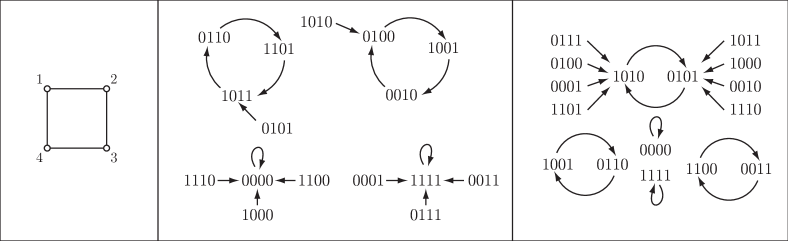
Figure 1: The graph $X=\mathrm{Circ}_{4}$ (left), and the phase spaces of $\mathbf{F}_{\pi}$ (middle) and $\mathbf{F}$ (right) for Example 2.1.

We remark that graph dynamical systems generalize concepts such as cellular automata and Boolean networks, and can describe a wide range of distributed, nonlinear phenomena.

3 $\omega$-Limit Set Structure of Bi-Threshold GDS

This section contains the two main results on dynamics of synchronous and asynchronous bi-threshold GDSs.

3.1 Synchronous Bi-Threshold GDSs

Let $K=\{0,1\}$ as before, let $A=(a_{ij})$ be a real-valued symmetric matrix, let $(k^{\uparrow}_{i})_{i=1}^{n}$ and $(k^{\downarrow}_{i})_{i=1}^{n}$ be vertex-indexed sequences of up- and down-thresholds, and define the function $\mathbf{F}=(f_{1},\dots,f_{n})\colon K^{n}\longrightarrow K^{n}$ by

$$f_{i}(x_{1},\dots,x_{n})=\begin{cases}1&\text{ if }x_{i}=0\text{ and }\sum\limits^{n}_{j=1}a_{ij}x_{j}\geq k^{\uparrow}_{i}\\ 0&\text{ if }x_{i}=1\text{ and }\sum\limits^{n}_{j=1}a_{ij}x_{j}<k^{\downarrow}_{i}\\ x_{i}&\text{ otherwise.}\end{cases}$$ (3.1)

The following theorem is a generalization of Theorem A.1 (see appendix) to the case of bi-threshold functions.

Theorem 3.1

If $\mathbf{F}$ is the synchronous GDS map over the complete graph of order $n$ with vertex functions as in Equation (3.1), then for all $x\in K^{n}$, there exists $s\in\mathbb{N}$ such that $\mathbf{F}^{s+2}(x)=\mathbf{F}^{s}(x)$.

The proof builds on the arguments of the proof from Goles and Olivos (1981) for standard threshold functions (see page A of the appendix). Note that we can use Lemma A.2 in its original form, but for Lemma A.4 changes are needed to adapt for bi-threshold functions. The position is marked [Cross-reference for bi-threshold systems] in the the proof of Lemma A.4 on page A.4. Before starting the proof of the theorem above, we first introduce the notion of bands and give a result on their structural properties. This is essential in the extension of the original result.

Let $z_{i}\in S$ and assume that $\gamma_{i}\geq 3$. As in the proof of Goles and Olivos (1981), we set

$$\operatorname{supp}(z_{i})=\bigl{\{}l\in\{0,1,2,\ldots,T-1\}:z_{l}=1\bigr{\}};\,$$

and use their partition $\mathcal{C}=\{C_{0},C_{1},C_{2},\ldots,C_{p}\}$. By the assumption $\gamma_{i}\geq 3$, we are guaranteed that $p\geq 1$. The bi-threshold functions require a more careful structural analysis of the elements of $\mathcal{C}$ than in the case of standard threshold functions. We say that $C\in\mathcal{C}$ is of type $ab$ if $z_{j}=a$ and $z_{j^{\prime}}=b$ where $j$ and $j^{\prime}$ are the indices immediately to the left and right of $C$, respectively (viewed modulo $T$). Here we write $m_{ab}=m_{ab}(\mathcal{C})$ for the number of elements of $\mathcal{C}$ of type $ab$.

We claim that $m_{01}=m_{10}$. Before we prove this, observe first that the sequence $\bigl{(}z_{i}(0),z_{i}(1),\ldots,z_{i}(T-1)\bigr{)}$ can be split into contiguous sub-sequences (bands) whose states contain only isolated 0s, where the end points have state 1, and where bands are separated by sub-sequences of lengths $\geq 2$ whose state consist entirely of 0s. By the construction of $\mathcal{C}$, each element $C\in\mathcal{C}$ must be fully contained in a single band. Our claim above is now a direct consequence of the following lemma:

Lemma 3.2

A band either ($i$) contains no element $C$ of type $01$ or $10$, or ($ii$) contains precisely one element $C$ of type $01$ and precisely one element $C^{\prime}$ of type $10$.

Proof 3.3.

Fix a band $B$ and let $C\in\mathcal{C}$ be the partition containing the initial element of B. There are now two possibilities. In the first case, $C$ also contains the final element of $B$. Then $C$ has type $00$, and any other partition element contained in $B$ is necessarily of type $11$. In the second case, $C$ terminates before the end of $B$. The configuration at the end of $C$ must then be as

and $C$ is of type $01$. The element $C^{\prime}$ containing the index after the last element of $C$ either goes all the way to the end of $B$, in which case it is of type $10$, or it terminates before that in which case the situation is as in the diagram above and $C^{\prime}$ is of type $11$. By repeated application of this argument, the band $B$ is eventually exhausted with an element $C^{\prime\prime}$ of type $10$. All other elements of $\mathcal{C}$ within $B$ not included in the sequence of partitions $C$, $C^{\prime}$ and so on, must be of type $11$, and the proof is complete.

Corollary 3.4.

$m_{01}(\mathcal{C})=m_{10}(\mathcal{C})$

Proof 3.5 ((Theorem 3.1)).

Claim: If $\gamma_{i}\geq 3$ for $z_{i}\in S$ then $\sum_{j=1}^{n}L(z_{i},z_{j})<0$.

We can write

$$\sum_{i=1}^{n}L(z_{i},z_{j})=\sum_{k=0}^{p}\Bigl{(}\sum_{j=1}^{n}a_{ij}\sum_{l\in C_{k}}\bigl{(}z_{j}(l+1)-z_{j}(l-1)\bigr{)}\Bigr{)}=\sum_{k=0}^{p}\Psi_{ik}\;,$$

where

$$\Psi_{ik}=\sum_{j=1}^{n}a_{ij}\sum_{l\in C_{k}}\bigl{(}z_{j}(l+1)-z_{j}(l-1)\bigr{)}=\sum_{j=1}^{n}a_{ij}z_{j}(l_{k}+2q_{k}+1)-\sum_{j=1}^{n}a_{ij}z_{j}(l_{k}-1)\;.$$

We need to consider $\Psi_{ik}$ for the four types of partition elements. As in the original proof, note that $\Psi_{i0}=0$.

$C_{k}$ is of type $00$: in this case $z_{i}(l_{k}-1)=0$, $z_{i}(l_{k})=1$, $z_{i}(l_{k}+2q_{k}+1)=0$ and $z_{i}(l_{k}+2q_{k}+2)=0$, which is only possible if

$$\sum_{j=1}^{n}a_{ij}z_{j}(l_{k}-1)\geq k^{\uparrow}_{i}\quad\text{and}\quad\sum_{j=1}^{n}a_{ij}z_{j}(l_{k}+2q_{k}+1)<k^{\uparrow}_{i}\;,$$

which implies that $\Psi_{ik}<0$.

$C_{k}$ is of type $11$: this case is completely analogous to the $00$ case, and again we conclude that $\Psi_{ik}<0$.

$C_{k}$ is of type $10$: here $z_{i}(l_{k}-1)=1$, $z_{i}(l_{k})=1$, $z_{i}(l_{k}+2q_{k}+1)=0$ and $z_{i}(l_{k}+2q_{k}+2)=0$. This implies that

$$\sum_{j=1}a_{ij}z_{j}(l_{k}-1)\geq k^{\downarrow}_{i}\quad\text{and}\quad\sum_{j=1}a_{ij}z_{j}(l_{k}+2q_{k}+1)<k^{\uparrow}_{i}\;,$$

leading to $\Psi_{ik}<k^{\uparrow}_{i}-k^{\downarrow}_{i}$.

$C_{k}$ is of type $01$: this case is essentially the same as the $10$ case, but here $\Psi_{ik}<k^{\downarrow}_{i}-k^{\uparrow}_{i}$.

Using the above four cases, we now have

$$\sum_{j=0}^{n}L(z_{i},z_{j})=\sum_{k=0}^{p}\Psi_{ik}<0+m_{00}\cdot 0+m_{11}\cdot 0+m_{10}(k^{\uparrow}_{i}-k^{\downarrow}_{i})+m_{01}(k^{\downarrow}_{i}-k^{\uparrow}_{i})=0\;,$$

where the last equality follows by Corollary 3.4. Clearly, this leads to the same contradiction as in the proof of Theorem A.1.

An immediate consequence of Theorem 3.1 is the following:

Corollary 3.6.

A synchronous bi-threshold GDS may only have fixed points and 2-cycles as limit sets.

3.2 Asynchronous Bi-Threshold GDSs

Theorem 3.7.

Let $X$ be a graph, let $\pi\in S_{x}$ and let $(f_{v})_{v}$ be bi-threshold functions all satisfying $\Delta(v)=k^{\downarrow}_{v}-k^{\uparrow}_{v}\leq 1$. The sequential dynamical system map $\mathbf{F}_{\pi}$ only has fixed points as limit sets.

As before, the graph $X$ is finite. Note also that the per-vertex thresholds $k^{\uparrow}$ and $k^{\downarrow}$ need not be uniform for the graph.

Proof 3.8.

The proof uses a potential function based on a construction in Barrett et al. (2006), but see also Goles-Chacc et al. (1985). For a given state $x\in K^{n}$ we assign to each vertex the potential

$$P(v,x)=\begin{cases}k^{\downarrow}_{v},&x_{v}=1\\ d(v)+2-k^{\uparrow}_{v},&x_{v}=0\;.\end{cases}$$

Note that the quantity $d(v)+2-k^{\uparrow}_{v}$ is the smallest number of vertex states in the local state $x[v]$ that must be zero to ensure that $x_{v}$ remains in state zero. Similarly, an edge $e=\{v,v^{\prime}\}$ is assigned the potential

$$P(e=\{v,v^{\prime}\},x)=\begin{cases}1,&x_{v}\neq x_{v^{\prime}}\\ 0,&x_{v}=x_{v^{\prime}}\;.\end{cases}$$

For book-keeping, we let $n_{i}=n_{i}(v;x)$ denote the number of vertices adjacent to $v$ in state $i$ for $i=0,1$ and note that $n_{0}+n_{1}=d$. The system potential $P(x)$ at the state $x$ is the sum of all the vertex and all the edge potentials. For the theorem statement it is clearly sufficient to show that each application of a vertex function that leads to a change in a vertex state causes the system potential to drop.

Consider first the case where $x_{v}$ is mapped from $0$ to $1$ which implies that $n_{1}\geq k^{\uparrow}_{v}$. Since a change in system potential only occurs for vertex $v$ and edges incident with $v$, we may disregard the other potentials when determining this change. Denoting the system potential before and after the update by $P$ and $P^{\prime}$, we have $P=d+2-k^{\uparrow}_{v}+n_{1}$ and $P^{\prime}=k^{\downarrow}_{v}+n_{0}$ which implies that

$$P^{\prime}-P =k^{\downarrow}_{v}+n_{0}-d-2+k^{\uparrow}_{v}-n_{1}=k^{\downarrow}_{v}+k^{\uparrow}_{v}-2n_{1}-2$$

$$\leq-(k^{\uparrow}_{v}-k^{\downarrow}_{v})-2=\Delta(v)-2\;,$$

and this is strictly negative whenever $\Delta=k^{\downarrow}-k^{\uparrow}\leq 1$. Similarly, for the transition where $x_{v}$ maps from $1$ to $0$ one must have $n_{1}+1\leq k^{\downarrow}_{v}-1$ or $n_{1}\leq k^{\downarrow}_{v}-2$. In this case we have

$$P^{\prime}-P =[d+2-k^{\uparrow}_{v}+n_{1}]-[k^{\downarrow}_{v}+n_{0}]=2n_{1}+2-k^{\downarrow}_{v}-k^{\uparrow}_{v}$$

$$\leq 2k^{\downarrow}_{v}-4+2-k^{\uparrow}_{v}-k^{\downarrow}_{v}=\Delta(v)-2$$

as before, concluding the proof.

3.3 Bifurcations in Asynchronous GDS

A natural question now is what happens in the case where $\Delta=k^{\downarrow}-k^{\uparrow}=2$ since periodic orbits are no longer excluded by the arguments in the proof above. The following proposition shows that there are graphs and choices of $k^{\uparrow}$ and $k^{\downarrow}$, such that $\Delta=2$, for which there are periodic orbits of arbitrary length.

Proposition 3.9.

The bi-threshold GDS map over $X=\mathrm{Circ}_{n}$ with update sequence $\pi=(1,2,3,\ldots,n)$, thresholds $k^{\uparrow}=1$ and $k^{\downarrow}=3$, has cycles of length $n-1$.

Proof 3.10.

We claim that the state $x=(0,0,\ldots,0,1,0)$ is on an $(n-1)$-cycle. Straightforward computations give that the single $1$-state is shifted one position to the left upon each application of $\mathbf{F}_{\pi}$ until the state $y=(0,1,0,\ldots,0)$ is reached. The image of this state is $z=(1,0,0,\ldots,0,0,1)$ which is easily seen to map to $x$. The smallest number of iterations required to return to the original state $x$ is $n-1$, producing a cycle as claimed.

In other words, by taking $\Delta$ as a parameter, we see that the bi-threshold sequential dynamical system undergoes a bifurcation at $\Delta=2$.

4 Dynamics of Bi-Threshold GDSs

4.1 Graph Unions

From Proposition 3.9, we see that for $X=\mathrm{Circ}_{n}$ with threshold $k^{\uparrow}=1$ and $k^{\downarrow}=3$ at each vertex, we obtain an $(n-1)$-cycle for the update sequence $\pi=(1,2,\dots,n)$. The following proposition demonstrates how we can combine graphs to obtain larger cycle sizes for bi-threshold SDSs with arbitrarily nonuniform $k^{\uparrow},k^{\downarrow}$. In particular, the result applies to the case where we combine $\mathrm{Circ}_{n}$ graphs where $p=n-1$ is prime.

Proposition 4.1.

For $i=1,2$ let $X_{i}$ be a graph for which the bi-threshold GDS with update sequence $\pi_{i}$ has a cycle in phase space of length $c_{i}$. Let $u_{i}\in\mathrm{v}[X_{i}]$, and let $X$ be the graph obtained as the disjoint union of $X_{1}$ and $X_{2}$ plus additionally the vertex $w\not\in\mathrm{v}[X_{1}],\mathrm{v}[X_{2}]$ with the edges $\{u_{1},w\}$ and $\{u_{2},w\}$. Moreover, let all thresholds of vertices in $X_{1}$ and $X_{2}$ be as before, and assign threshold $k^{\uparrow}=3$ to $w$. The bi-threshold SDS map over $X$ with update sequence $\pi=(\pi_{1}|\pi_{2}|w)$ [juxtaposition] has a cycle of length $\operatorname{lcm}(c_{1},c_{2})$.

Proof 4.2.

Let vertex $w$ have $k^{\uparrow}=3$, so that $w$ will never transition to state $1$ from state $0$. Let $x=(x_{1}|x_{2}|x_{w})$ be the state over $X$ constructed from states $x_{1}$ and $x_{2}$ on the respective $c_{i}$-cycle over $X_{1}$ and $X_{2}$ with $x_{w}=0$. The only vertices whose connectivity, and therefore induced vertex function, are affected by the addition of $w$ are $u_{1}$ and $u_{2}$. But the state transitions for $u_{1}$ and $u_{2}$ are unaffected because each is predicated on $\sigma(x[u_{1}])$ and $\sigma(x[u_{2}])$, respectively, and these latter two quantities are not altered by the state of $w$ because that state is fixed at $0$ by construction. Hence, the phase space of $X$ contains a cycle of length $\operatorname{lcm}(c_{1},c_{2})$ as claimed.

Thus, for $k^{\uparrow}=1$ and $k^{\downarrow}=3$, there exists a circle graph and permutation $\pi$ that will produce a cycle in phase space of length three or greater, and multiple circle graphs can be combined to produce graphs with large orbit cycles without modifying the thresholds of vertices in $X_{1}$ and $X_{2}$.

4.2 Trees

Propositions 3.9 and 4.1 show how periodic orbits of length $>2$ arise over graphs that contain cycles. This section investigates bi-threshold SDS maps where $X$ is a tree.

To start, we first recall the notion of $\kappa$-equivalence of permutations from Macauley and Mortveit (2009, 2008). Two permutations $\pi,{\pi^{\prime}}\in S_{X}$ are $\kappa$-equivalent if the corresponding induced acyclic orientations $O_{\pi}$ and $O_{\pi^{\prime}}$ of $X$ are related by a sequence of source-to-sink conversions. Here, the orientation $O_{\pi}$ is obtained from $\pi$ by orienting each edge $\{v,v^{\prime}\}\in\mathrm{e}[X]$ as $(v,v^{\prime})$ if $v$ precedes $v^{\prime}$ in $\pi$ and as $(v^{\prime},v)$ otherwise. This is an equivalence relation, and it is shown in Macauley and Mortveit (2009) that ($i$) for a tree the number of $\kappa$-equivalence classes is $\kappa(X)=1$, and ($ii$) that $\mathbf{F}_{\pi}$ and $\mathbf{F}_{\pi^{\prime}}$ have the same periodic orbit structure (up to digraph isomorphism/topological conjugation) whenever $\pi$ and ${\pi^{\prime}}$ are $\kappa$-equivalent. As a result, we only need to consider a single permutation update sequence to study the possible periodic orbit structures of permutation SDS maps over a tree $X$.

The following result shows that there can be cycles of length $3$ or greater for permutation SDS over a tree.

Proposition 4.3.

For any integer $c\geq 3$ there is a tree $X$ on $n=4c-6$ vertices such that bi-threshold permutation SDS maps over $X$ with thresholds $k^{\uparrow}=1$ and $k^{\downarrow}=3$ have periodic orbits of length $c$.

Proof 4.4.

An $H$-tree on $n=4\beta+2$ vertices, denoted by $H_{n}$, has vertex set $\{1,2,\ldots,n\}$ and edge set

$$\{\eta,n-\eta+1\}\cup\bigl{\{}\{i,i+1\},n/2+\{i,i+1\}\mid 1\leq i\leq n/2-1\bigr{\}}\;,$$

where $\eta=\beta+1$ and $\beta\geq 1$. The graph $H_{n}$ is illustrated in Figure 2.

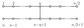
Figure 2: The tree $H_{n}$ used in the proof of Proposition 4.3.

Set $\beta=c-2$ so that $n=4\beta+2$ and $\eta=\beta+1$. We take $X=H_{n}$ as the graph and assign thresholds $(k^{\uparrow},k^{\downarrow})=(1,3)$ to all vertices. By the comment preceding Proposition 4.1, we may simply use $\pi=(1,2,3,\ldots,n)$ as update sequence since all permutations give cycle equivalent maps $\mathbf{F}_{\pi}$.

For the initial configuration, set the state of each vertex $v$ in the range $(n/2)+1\leq v\leq n-\eta+1$ (bottom right branch) to $1$ and set all other vertex states to $0$ so that

$$x(0)=(0,0,\dots,0,\underbrace{1,1,\dots,1,}_{{\text{start at vertex $(n/2)+1$}}}0,0,\dots 0)$$

The number of vertices in a contiguous vertex range with state 1 will always be $\eta$; there may be one or two such groups in a system state. The image of $x(0)$ is

$$x(1)=(0,0,\dots,0,\underbrace{1,1,\dots,1,}_{\text{start at vertex $\eta$}}0,0,\dots 0)\;,$$

where now the first $\eta-1$ vertices are in state 0, the next $\eta$ vertices are in state 1, and the remaining vertices—all those along the bottom arm—are in state 0, as follows. Along the top arm, vertices $1$ through $\eta-1$ will remain in state $0$ because all nodes and their neighbors are in state $0$. Vertex $\eta$, the state of the vertex incident to the crossbar on the top arm, will change to $1$ because its neighbor along the crossbar is in state $1$. For the given permutation, then, each subsequent vertex $v_{i}$ in the range $\eta+1$ through $n/2$ will change to state $1$ because $x_{v_{i-1}}=1$ and $k^{\uparrow}=1$. For the bottom arm, vertex $(n/2)+1$ will change from state 1 to state 0 because $\sigma(x[v_{(n/2)+1}])=2<k^{\downarrow}$. For the same reason, each vertex $v_{i}$ in the range $(n/2)+2$ to $n-\eta+1$ will transition to state 0. Vertices from $n-\eta+2$ through $n$ will remain in state 0.

The next state is

$$x(2)=(0,0,\dots,0,\underbrace{1,1,\dots,1}_{\text{start at vertex }\eta-1},0,0,\ldots 0,\underbrace{1,1,\dots,1}_{\text{start at vertex }n-\eta+1})\;,$$

where, for the top arm, the first $\eta-2$ vertices are in state 0, the next $\eta$ vertices are in state 1, and the last vertex on the top arm is in state 0. That is, the set of 1’s along the top arm has shifted one vertex left, as follows. Let the set of vertices in the top arm in state 1 (in $x(1)$) be denoted $v_{i}$ through $v_{i+\eta}$. Vertex $v_{i-1}$ will transition $0\rightarrow 1$ because $x_{v_{i}}=1$. Vertex $v_{i}$ will remain in state 1 because $\sigma(x[v_{i}])=3=k^{\downarrow}$. Likewise $v_{i+1}$ through $v_{i+\eta-1}$ will remain in state 1. However, $v_{i+\eta}$ will transition to state 0 because $\sigma(x[v_{i+\eta}])=2<k^{\downarrow}$. We refer to this behavior as a left-shift (the analogous shift to the right is a right-shift). For the bottom arm, the $\eta$ vertices (labels $(n/2)+1$ through $n-\eta$) remain in state 0. Vertex $n-\eta+1$ transitions to state 1 because the neighbor along the crossbar is in state 1. Subsequently, vertices $n-\eta+2$ through $n$ transition to state 1, in turn, according to $\pi$.

The next state is

$$x(3)=(0,0,\ldots,0,\underbrace{1,1,\dots,1}_{\text{start at vertex }\eta-2},0,0,\ldots 0,\underbrace{1,1,\dots,1}_{\text{start at vertex }n-\eta})\;,$$

where the set of $\eta$ vertices in state 1 in the top arm has shifted left, and the set of $\eta$ vertices in state 1 in the bottom arm has shifted left. The shifting process embodied in the transition from state $x(2)$ to $x(3)$—where there is a group of vertices in state 1 in each of the top and bottom arms—can happen a total of $(\eta-2)$ times. The state after these $(\eta-2)$ transitions is

$$x(\eta)=(\underbrace{1,1,\dots,1}_{\text{start at vertex 1}},0,0,\ldots 0,\underbrace{1,1,\dots,1,}_{\text{start at vertex }n-2\eta+3}0,0,\ldots,0)\;.$$

The image of $x(\eta)$ is $x(0)$, the initial state. There are $2+(\eta-2)+1$ state transitions, and we have a limit cycle of length $c=\eta+1$.

Of course, the proof does not guarantee that $c$ is the minimal periodic orbit size, nor that $H_{n}$ is the minimal order tree with a periodic orbit of this length. Additionally, there may be multiple periodic orbits of length $c$. The following proposition expands on this in the case where $c\geq 5$: there exists a tree of smaller order than $H_{n}$ that also admits a $c$-cycle, namely the $Y$-trees.

Proposition 4.5.

For any integer $c\geq 3$ there is a tree on $n=3c-2$ vertices such that bi-threshold permutation SDS maps over this tree with thresholds $k^{\uparrow}=1$ and $k^{\downarrow}=3$ have periodic orbits of length $c$.

Proof 4.6.

The proof is analogous to the case of the $H$-tree. We take as the graph the $Y$-tree on $n=3\beta+1$ vertices (see Figure 3) with $\beta\geq 1$, which has vertex set $\{1,2,\ldots,n\}$ and, setting $\eta=\beta+1$, edge set

$$\bigl{\{}\{i,i+1\}\mid 1\leq i\leq 2\eta-2\bigr{\}}\cup\bigl{\{}\{i,i+1\}\mid 2\eta\leq i\leq(n-1)\bigr{\}}\cup\{\eta,n\}\;.$$

Figure 3: The tree $Y_{n}$ used in the proof of Proposition 4.5.

Let $c\geq 3$ with $n=3c-2$ so that $X=Y_{n}$ (and $c=\beta+1$). We assign thresholds $(k^{\uparrow},k^{\downarrow})=(1,3)$ to all vertices and use update sequence $\pi=(1,2,3,\ldots,n)$ as before. As the initial configuration, set the states of the $\beta$ vertices $v$ in the range $\eta\leq v\leq 2\eta-2$ (all vertices in the upper right branch except $2\eta-1$) to $1$, and set all other vertex states to $0$ to form

$$x(0)=(0,0,\ldots,0,\underbrace{1,1,\dots,1,}_{\text{start at vertex $\eta$}}0,0,\dots 0)\;.$$

The image of $x(0)$ is

$$x(1)=(0,0,\dots,0,\underbrace{1,1,\dots,1,}_{\text{start at vertex $(\eta-1)$}}0,0,\dots 0,1)\;,$$

where now the first $\eta-2$ vertices are in state $0$, the next $\beta$ vertices are in state 1, and the remaining vertices—except for vertex $n$—are in state $0$. In the upper two branches, the initial set of $\beta$ nodes in state $1$ shifts left for the same reasons described in the proof of Proposition 4.3. The last vertex, $n$, will change to $1$ because it is adjacent to vertex $\eta$, which has state $1$.

The image of $x(1)$ is

$$x(2)=(0,0,\ldots,0,\underbrace{1,1,\dots,1,}_{\text{start at vertex $(\eta-2)$}}0,0,\ldots 0,1,1)\;,$$

where the $\beta$ nodes in state $1$ beginning at vertex $\eta-2$ have shifted left and vertex $n-1$ transitions to $1$ because vertex $n$ is in state $1$. Vertex $n$ remains in state 1 because $\sigma(x[v_{n}])=3$.

The mechanics of the last state transition (the left shift of $\beta$ vertices and nodes transitioning to state $1$ in the lower branch) repeats itself a total of $\beta-2$ times, at which point the state is

$$x(\beta-1)=(0,1,\dots,1,\underbrace{0,0,\dots,0,}_{\text{start at vertex $(\eta+1)$}}\underbrace{1,1,\dots,1}_{\text{start at vertex $(n-\beta+2)$}})\;,$$

where the only vertex in the lower vertical branch in state $0$ is $2\eta$, the leaf node.

Noting that vertex $\eta$ remains in state $1$ on the next transition because $\sigma(x[v_{\eta}])=3$, all vertices in the upper right branch transition to $1$. Vertex $2\eta$ also transitions to $1$, giving

$$x(\beta)=(1,1,\ldots,1)\;.$$

The next state can be verified to be $x(0)$, thus completing the cycle. The cycle length is therefore $c=\beta+1$ as stated.

Interestingly, there is no $H$-tree nor $Y$-tree that generates a maximum orbit of size 2 for thresholds $(k^{\uparrow},k^{\downarrow})=(1,3)$. However, so-called $X$-trees (defined below) admit cycles of any size $c\geq 1$.

Proposition 4.7.

For any integer $c\geq 2$ there is a tree $X$ on $n=4c-3$ vertices such that bi-threshold permutation GDS maps over $X$ with thresholds $k^{\uparrow}=1$ and $k^{\downarrow}=3$ have periodic orbits of length $c$. For $c=1$, there is a tree $X$ on $n=5$ vertices that has periodic orbits of length 1 (fixed points).

Proof 4.8.

An $X$-tree on $n=4\beta+1$ vertices with $\beta\geq 1$ has vertex set $\{1,2,\ldots,n\}$ and edge set as illustrated in Figure 4. Here $\eta=\beta+1$ is the unique vertex of degree 4.

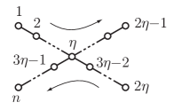
Figure 4: The tree $X_{n}$ used in the proof of Proposition 4.7 (arrows indicate vertex labeling order).

Note first that for any $n$ the all-zero state over $X_{n}$ is a fixed point.

We treat the case $c=2$ separately; use $X=X_{5}$, $\pi=(1,2,3,4,5)$, and $(k^{\uparrow},k^{\downarrow})=(1,3)$. It can easily be verified that $x(0)=(0,1,1,0,0)$ is mapped to $x(1)=(1,1,0,1,1)$ which in turn is mapped to $x(0)$, constituting a $2$-cycle.

Fix $c\geq 3$, set $n=4c-3$ and then $c=\beta+1$, take as the graph $X=X_{n}$ with thresholds $(k^{\uparrow},k^{\downarrow})=(1,3)$ for all vertices, and let $\pi=(1,2,3,\ldots,n)$.

Define the initial configuration $x(0)$ by assigning the $\beta$ vertices $v$ with $\eta\leq v\leq 2\eta-2$ (all vertices in the upper right branch except $2\eta-1$) to $1$ and set all other vertex states to $0$, that is,

$$x(0)=(0,0,\dots,0,\underbrace{1,1,\dots,1,}_{\text{start at vertex $\eta$}}0,0,\dots 0)\;.$$

The image of $x(0)$ is

$$x(1)=(0,0,\dots,0,\underbrace{1,1,\dots,1,}_{\text{start at vertex $(\eta-1)$}}0,0,\dots 0,\underbrace{1,1,\dots,1}_{\text{start at vertex $3\eta-2$}})\;,$$

where now the first $\eta-2$ vertices are in state 0, the next $\beta$ vertices are in state 1, and the remaining vertices in branch 2 are in state $0$. In branch 3, only the vertex neighboring vertex $\eta$ transitions to state $1$, while all vertices in branch 4 transition to state $1$ because $\eta$ is in state $1$.

State $x(2)$ is generated by a left-shift of the $\beta$ contiguous states that are 1 in branches 1 and 2, and by a left-shift of the $\beta+1$ contiguous state-1 vertices in branches 3 and 4, that is,

$$x(2)=(0,0,\ldots,0,\underbrace{1,1,\dots,1,}_{\text{start at vertex $(\eta-2)$}}0,0,\ldots 0,\underbrace{1,1,\dots,1,}_{\text{start at vertex $3\eta-3$}}0)\;.$$

From $x(1)$ there are $\beta-2$ such transitions that result in the state

$$x(\beta-1)=(0,\underbrace{1,1,\dots,1,}_{\text{start at vertex $2$}}0,0,\dots 0,\underbrace{1,1,\dots,1,}_{\text{start at vertex $3\eta-\beta$}}0,0,\dots,0)\;.$$

The next transition results in all vertices in branches 1 and 2 in state $1$ since $\eta$ remains in state 1. The contiguous set of $\beta+1$ vertices in branches 3 and 4 shift left, giving

$$x(\beta)=(1,1,\dots,1,\underbrace{0,0,\dots,0}_{\text{start at vertex $3\eta$}})\;.$$

The image of $x(\beta)$ is $x(0)$, and, since $\beta$ is the smallest positive time step with this property, we have established the presence of a periodic orbit of length $c=\beta+1$.

Finally, we consider a special class of bi-threshold SDSs on trees with $k^{\uparrow}=1$ and $k^{\downarrow}=k^{\downarrow}(v)=d(v)+1$ for each vertex $v$. Note that the down-threshold for each vertex depends on its degree as indicated by the index $v$ in $k^{\downarrow}(v)$. We show that such bi-threshold SDS maps always have fixed points. In such systems, the state of a vertex $v$ switches from 0 to 1 if it has at least one neighbor in state 1, and from 1 to 0 if it has at least one neighbor in state 0. This is an interesting contrast to the classes of bi-threshold SDSs on trees discussed above which have large limit cycles.

Let $X$ be a tree. We choose some arbitrary vertex $r\in v[X]$ as its root, and partition $X$ into levels $X_{0},X_{1},\ldots,X_{D}$ with respect to $r$ such that $X_{0}=\{r\}$, and for any $i\geq 0$, we let $X_{i+1}$ be the set of vertices adjacent to vertices in set $X_{i}$, but not in the set $\cup_{j<i}X_{j}$. We sometimes refer to $X_{i}$ as level-$i$ set. Let $D$ be the number of levels. We can also define a parent-child relationship relative to this rooted tree, and denote $p(v)$ as the parent of vertex $v\neq r$. In our arguments below, we use any permutation $\pi$ of $v[X]$, which consists of all the vertices in $X_{i}$ before those in $X_{i-1}$ for each $i$. Our result is based on the following property.

Lemma 4.9.

Consider a bi-threshold SDS $\mathbf{F}_{\pi}$ on a tree $X$ with an arbitrary root $r$ and permutation $\pi$ as defined above where $k^{\uparrow}=1$ and $k^{\downarrow}(v)=d(v)+1$ for each vertex $v$. Let $x$ be any state vector and $x^{\prime}=\mathbf{F}_{\pi}(x)$. For each vertex $v$ other than the root, we have $x^{\prime}_{v}=x_{p(v)}$.

Proof 4.10.

Our proof is by induction on the levels, starting from the highest, i.e., $X_{D}$. For the base case, consider a leaf $v\in X_{D}$. We have four cases: $x_{v}=x_{p(v)}=1$, $x_{v}=0,x_{p(v)}=1$, $x_{v}=1,x_{p(v)}=0$ and $x_{v}=x_{p(v)}=0$. It is easy to verify that in the first two cases, we have $x^{\prime}_{v}=1$ and in the latter two cases, we have $x^{\prime}_{v}=0$, since vertex $v$ is updated before $p(v)$ in $\pi$. Therefore, the statement of the lemma holds in the base case for all vertices $v\in X_{D}$.

Next, consider a vertex $v$ in some level $X_{j}$, $j<D$. If $v$ is a leaf in $X_{j}$, the lemma follows by exactly the same argument as in the base case. Therefore, consider the case $v$ is not a leaf. Let $w_{1},\ldots,w_{c}$ denote its children. Since level $j+1$ vertices are updated before those in level $j$ in $\pi$, by induction, we have $x^{\prime}_{w_{i}}=x_{v}$ for each $w_{i}$. Again, we have a case similar to the base case: when vertex $v$ is updated, it has the same values as its children, and therefore, takes on the state of $p(v)$. Thus, the lemma follows.

This property immediately gives us the following:

Corollary 4.11.

Let $X$ be a tree. Let $\pi\in S_{x}$ and let $(f_{v})_{v}$ be bi-threshold functions satisfying $k^{\uparrow}=1$ and $k^{\downarrow}(v)=d(v)+1$ for each vertex $v$. Any SDS map $\mathbf{F}_{\pi}$ only has fixed points as limit sets.

Proof 4.12.

Without loss of generality, we take $\pi$ to be the permutation in Lemma 4.9. By applying Lemma 4.9, it is easy to verify that for any state vector $x$, all the vertices in levels 0 and 1 have the same state value in $F(x)$, namely $x_{r}$. By induction on $i$, it is easy to verify that for any $i\geq 1$, all vertices in levels $0,\ldots,i$ have the same state value (of $x_{r}$) in $F^{i}(x)$. The statement follows since all permutations for a tree give cycle equivalent SDS maps.

5 Summary and Conclusion

This paper has analyzed the structure of $\omega$-limit sets of bi-threshold GDS. Unlike the synchronous case, bi-threshold SDS maps can have long periodic orbits, and this is characterized in terms of the difference of the up- and down-thresholds. We also analyzed certain classes of trees. The following is a list of questions and conjectures for possible further research.

5.1 Embedding and Inheritance of Dynamics

A fundamental question in the study of GDSs is the following: if a graph $X$ has a graph $X^{\prime}$ as an induced subgraph, what are the relations between the dynamics over the two graphs? Here one has to assume that the vertex function, and update sequences if applicable, are appropriately related. For example, is there a projection from the phase space of the GDS over $X$ to the one over $X^{\prime}$?

In initial computational experiments we studied the dynamics for bi-threshold GDS over trees obtained from, e.g. $H$-trees by adding a collection of edges - results indicate that there are several classes of outcomes. While this is hardly a surprise, there are clear patterns in how edges are added and the dynamics that result. For example, some classes of edge additions give trees that have long periodic orbits just as in the case of $H$-trees. For other classes of edge additions, however, the addition of even a single edge causes all periodic orbits of size $\geq 2$ to disappear. Further insight into the mechanisms involved could shed light on the the fundamental question above.

5.2 Minimality of Trees with Given Periodic Orbit Sizes

Our results above on the existence of trees admitting bi-threshold SDS with given periodic orbit sizes are not necessarily minimal. For a given $c\geq 1$ there is an $X$-tree with a periodic orbit of length $c$, but there may be a smaller tree (or graph in general) which admits periodic orbits of size $c$ as well. While we have obtained some insight on this via sampling, no firm results have been established.

Note. For all computational experiments involving dynamics of SDS maps over graphs in this paper we used a variant of InterSim (Kuhlman et al., 2011).

Appendix A Limit Cycle Structure for Standard Threshold Cellular Automata

This appendix section contains a condensed version of the proof from Goles and Olivos (1981) for standard threshold functions. We have incorporated their proof for two reasons. First, only a portion of the original proof needs to be adapted to cover bi-threshold systems, and in this way the paper becomes self-contained. Second, the original proof only appears in French, and we here provide an English version.

Let $K=\{0,1\}$, let $A=(a_{ij})_{i,j=1}^{n}$ be a real symmetric matrix, let $\theta=(\theta_{1},\dots,\theta_{n})\in\mathbb{R}^{n}$, and let $\mathbf{F}=(f_{1},\ldots,f_{n})\colon K^{n}\longrightarrow K^{n}$ be the function defined coordinate-wise by

$$f_{i}(x_{1},\ldots,x_{n})=\begin{cases}0,&\text{if }\sum\limits^{n}_{j=1}a_{ij}x_{j}<\theta_{i}\\ 1,&\text{otherwise}\;.\end{cases}$$ (A.1)

Theorem A.1.

For all $x\in K^{n}$, there exists $s\in\mathbb{N}$ such that $\mathbf{F}^{s+2}(x)=\mathbf{F}^{s}(x)$.

The proof of this theorem is based on two lemmas which are given below. Note first that since $K^{n}$ is finite, for each $x\in K^{n}$ there exist $s,T\in\mathbb{N}$ (they will generally depend on $x$) with $T>0$ such that

$$\mathbf{F}^{s+T}(x)=\mathbf{F}^{s}(x)\quad\text{and}\quad\mathbf{F}^{s+r}(x)\neq\mathbf{F}^{s}(x)$$

for all $0<r<T$. Here $s$ is the transient length of the state $x$. Next define the $n\times T$ matrix $X(x,T)=(\mathbf{F}^{s}(x),l\dots,\mathbf{F}^{s+T-1}(x))$ by

$$X(x,T)=\left(\begin{array}[]{ccc}z_{1}(0)&\dots&z_{1}(T-1)\\ \vdots&\cdots&\vdots\\ z_{n}(0)&\dots&z_{n}(T-1)\end{array}\right)\;,$$

where $\mathbf{F}^{s}(x)=z=(z_{1}(0),\dots,z_{n}(0))$ and $\mathbf{F}^{s+T-1}(x)=(z_{1}(T-1),\dots,z_{n}(T-1))$. In other words, $z$ denotes the first periodic point reached from $x$ (after $s$ steps) and its period is $T$. The columns of $X(x,T)$ are the $T$ successive periodic points of the cycle containing $z$.

In general we have

$$\mathbf{F}^{s+l}(x)=(z_{1}(l),\dots,z_{n}(l))\text{ for }0\leq l\leq T-1\;.$$

Since

$$\mathbf{F}^{s}(x)=\mathbf{F}^{s+T}(x)=\mathbf{F}(z_{1}(T-1),\ldots,z_{n}(T-1))$$

we have $z_{i}(0)=f_{i}(z_{1}(T-1),\ldots,z_{n}(T-1))$, and from $\mathbf{F}^{s+l+1}(x)=\mathbf{F}(\mathbf{F}^{s+l}(x))$ we have

$$z_{i}(l+1)=f_{i}(z_{1}(l),\dots,z_{n}(l))\text{ for }l=0,\ldots,T-2.$$

We will call $z_{i}$ the $i{}^{\text{th}}$ row of the matrix $X(x,T)$ and let $\gamma_{i}$ denote the smallest divisor of $T$ such that $z_{i}(l+\gamma_{i})=z_{i}(l)$ for $l\in\{0,\dots,T-1\}$, and will say that $\gamma_{i}$ is the period of the component $z_{i}$. Clearly, we have $z_{i}(l+T)=z_{i}(l)$ for $i\in\{1,2,\ldots,n\}$ and all $l\in\{0,\dots,T-1\}$. Let $S=\{z_{1},\dots,z_{n}\}$ be the set of rows of $X(x,T)$. We define the operator $L\colon S\times S\rightarrow\mathbb{R}$ by

$$L(z_{i},z_{j})=a_{ij}\sum^{T-1}_{l=0}(z_{j}(l+1)-z_{j}(l-1))z_{i}(l)\;,$$

with indices taken modulo $T$.

Lemma A.2.

The operator $L$ has the following properties:

• $L(z_{i},z_{j})+L(z_{j},z_{i})=0$ for $i,j\in\{1,\ldots,n\}$ (anti-symmetry).

• If $\gamma_{i}\leq 2$ then $L(z_{i},z_{j})=0$ for $j\in\{1,\ldots,n\}$.

Proof A.3.

For ($i$), since $a_{ij}=a_{ji}$, we have

$$L(z_{i},z_{j})+L(z_{j},z_{i})=a_{ij}\sum^{T-1}_{l=0}\bigl{(} [z_{i}(l)z_{j}(l+1)-z_{i}(l-1)z_{j}(l)]$$

$$+ [z_{i}(l+1)z_{j}(l)-z_{i}(l)z_{j}(l-1)]\bigr{)}\;,$$

which clearly evaluates to zero due to periodicity. For part ($ii$), if $\gamma_{i}=1$ then the row $z_{i}$ is constant and $L(z_{i},z_{j})=0$. If $\gamma_{i}=2$ then the value of $z_{i}$ alternates as

$$z_{i}(0),z_{i}(1),z_{i}(0),z_{i}(1),\ldots,z_{i}(0),z_{i}(1)$$

across the $i^{\text{th}}$ row, and the terms in $L(z_{i},z_{j})$ cancel in pairs.

Let $z_{i}\in S$ and suppose in the following that $\gamma_{i}\geq 3$. We set

$$\operatorname{supp}(z_{i})=\{l\in\{0,\ldots,T-1\}:z_{i}(l)=1\}\;,$$

and write $\mathcal{I}(l)=\{l,l+2,l+4,\ldots,l-4,l-2\}$. Next, set

$$C_{0}=\begin{cases}\varnothing,&\text{ if there is no }l_{0}\in\{0,\dots,T-1\}\text{ such that }\mathcal{I}(l_{0})\subset\operatorname{supp}(z_{i})\\ \mathcal{I}(l_{0}),&\text{otherwise}.\end{cases}$$

We define $C_{1}$ as the set

$$C_{1}=\{l_{1}+2s\in\operatorname{supp}(z_{i}):s=0,1,\ldots,q_{1}\}\;,$$

where $l_{1}$ is the smallest index not in $C_{0}$ satisfying $z_{i}(l_{1}-2)=0$ and $q_{1}$ satisfies $z_{i}(l_{1}+2q_{1}+2)=0$. For $k\geq 2$ we define the sets $C_{k}$ by

$$C_{k}=\{l_{k}+2s\in\operatorname{supp}(z_{i}):s=0,1,\dots,q_{k}\}\;,$$

where $l_{k}=l_{k-1}+r\pmod{T}\notin\{l_{1},\ldots,l_{k-1}\}$ is the smallest index for which $z_{i}(l_{k}-2)=0$ and $q_{k}$ satisfies $z_{i}(l_{k}+2q_{k}+2)=0$.

Since $\gamma_{i}\geq 3$ (assumption), there always exists $l_{1}\in\operatorname{supp}(z_{i})$ for which $z_{i}(l_{1}-2)=0$. This allows us to build the collection of sets $\mathcal{C}=\{C_{0},\dots,C_{p}\}$. By construction, $\mathcal{C}$ is a partition of $\operatorname{supp}(z_{i})$. The following lemma provides the final piece needed in the proof of the main result.

Lemma A.4.

For $z_{i}\in S$ and with $\gamma_{i}\geq 3$ we have

$$\sum^{n}_{j=1}L(z_{i},z_{j})<0\;.$$

Proof A.5.

Using the partition $\mathcal{C}$ of $\operatorname{supp}(z_{i})$, we have

$$\sum^{n}_{j=1}L(z_{i},z_{j}) =\sum^{n}_{j=1}a_{ij}\sum_{l\in\operatorname{supp}(z_{i})}(z_{j}(l+1)-z_{j}(l-1))\cdot 1$$

$$=\sum^{n}_{j=1}a_{ij}\sum^{p}_{k=0}\sum_{l\in C_{k}}(z_{j}(l+1)-z_{j}(l-1))=\sum^{p}_{k=0}\sum^{n}_{j=1}a_{ij}\sum_{l\in C_{k}}(z_{j}(l+1)-z_{j}(l-1))$$

$$=\sum^{p}_{k=0}\Psi_{ik}\;,$$

where we have introduced

$$\Psi_{ik}=\sum^{n}_{j=1}a_{ij}\sum_{l\in C_{k}}(z_{j}(l+1)-z_{j}(l-1))\;.$$ (A.2)

If $C_{0}=\varnothing$ then $\Psi_{i0}=0$, and if $C_{0}=\{l_{0},l_{0}+2,\ldots,l_{0}-2\}$ we have

$$\sum_{l\in C_{0}}(z_{j}(l+1)-z_{j}(l-1))=0\;.$$

In other words, we always have $\Psi_{i0}=0$, so we assume $k>0$ in the following. From the assumption that $\gamma_{i}\geq 3$, there exists $C_{k}\neq\varnothing$ such that $C_{k}=\{l_{k},l_{k}+2,\ldots,l_{k}+2q_{k}\}$, so we can re-write $\Psi_{ik}$ as

$$\Psi_{ik} =\sum^{n}_{j=1}a_{ij}\sum_{s=0}^{q_{k}}(z_{j}(l_{k}+2s+1)-z_{j}(l_{k}+2s-1))$$

$$=\sum^{n}_{j=1}a_{ij}z_{j}(l_{k}+2q_{k}+1)-\sum^{n}_{j=1}a_{ij}z_{j}(l_{k}-1)\;.$$

[Cross-reference for bi-threshold systems] By the construction of $C_{k}$, we have $z_{i}(l_{k}+2q_{k}+2)=0$ and $z_{i}(l_{k})=1$ which, by the definition of $f$ in (A.1), is only possible if

$$\sum^{n}_{j=1}a_{ij}z_{j}(l_{k}+2q_{k}+1)<\theta_{i},\quad\text{and}\quad\sum^{n}_{j=1}a_{ij}z_{j}(l_{k}-1)\geq\theta_{i}\;.$$ (A.3)

This implies that $\Psi_{ik}<0$ and we conclude that

$$\sum^{n}_{j=1}L(z_{i},z_{j})=\sum^{p}_{k=1}\Psi_{ik}<0\;$$

as required.

Proof A.6 (of Theorem A.1).

From Lemma A.2 we have that $L$ is anti-symmetric so

$$\sum^{n}_{i=1}\sum^{n}_{j=1}L(z_{i},z_{j})=0\;.$$

However, if we assume that $T\geq 3$, then there is $z_{i}$ with $\gamma_{i}\geq 3$ and Corollary 3.4 produces the desired contradiction. We conclude that $T\leq 2$.

References

- Atkinson et al. (1994) R. Atkinson, W. Dietz, J. Foreyt, N. Goodwin, J. Hill, J. Hirsch, F. Pi-Sunyer, R. Weinsier, R. Wing, J. Hoofnagle, J. Everhart, V. Hubbard, and S. Yanovski. Weight Cycling. Journal of the American Medical Association, 272(15):1196–1202, 1994.
- Barrett et al. (2006) C. L. Barrett, H. B. Hunt III, M. V. Marathe, S. S. Ravi, D. J. Rosenkrantz, and R. E. Stearns. Complexity of reachability problems for finite discrete sequential dynamical systems. Journal of Computer and System Sciences, 72:1317–1345, 2006.
- Bischi and Merlone (2009) G. Bischi and U. Merlone. Global Dynamics in Binary Choice Models with Social Influence. J. Math. Sociology, 33:277–302, 2009.
- Bulger et al. (1989) N. Bulger, A. DeLongis, R. Kessler, and E. Wethington. The Contagion of Stress Across Multiple Roles. Journal of Marriage and the Family, 51:175–183, 1989.
- Centola and Macy (2007) D. Centola and M. Macy. Complex Contagions and the Weakness of Long Ties. American J. Sociology, 113(3):702–734, 2007.
- Christakis and Fowler (2007) N. Christakis and J. Fowler. The Spread of Obesity in a Large Social Network Over 32 Years. N. Engl. J. Med., pages 370–379, 2007.
- Goles and Olivos (1981) E. Goles and J. Olivos. Comportement periodique des fonctions a seuil binaires et applications. Discrete Applied Mathematics, 3:93–105, 1981.
- Goles-Chacc et al. (1985) E. Goles-Chacc, F. Fogelman-Soulie, and D. Pellegrin. Decreasing energy functions as a tool for studying threshold networks. Discrete Applied Mathematics, 12:261–277, 1985.
- Granovetter (1978) M. Granovetter. Threshold Models of Collective Behavior. American J. Sociology, 83(6):1420–1443, 1978.
- Karaoz et al. (2004) U. Karaoz, T. Murali, S. Letovsky, Y. Zheng, C. Ding, C. R. Cantor, and S. Kasif. Whole-genome annotation by using evidence integration in functional-linkage networks. Proceedings of the National Academy of Sciences, 101(9):2888–2893, 2004.
- Kauffman (1969) S. A. Kauffman. Metabolic stability and epigenesis in randomly constructed genetic nets. Journal of Theoretical Biology, 22:437–467, 1969.
- Kempe et al. (2003) D. Kempe, J. Kleinberg, and E. Tardos. Maximizing the Spread of Influence Through a Social Network. In Proc. ACM KDD, pages 137–146, 2003.
- Kuhlman et al. (2011) C. Kuhlman, V. Kumar, M. Marathe, H. Mortveit, S. Swarup, G. Tuli, S. Ravi, and D. Rosenkrantz. A General-Purpose Graph Dynamical System Modeling Framework. In Proceedings of the 2011 Winter Simulation Conference (WSC 2011), 2011.
- Macauley and Mortveit (2008) M. Macauley and H. S. Mortveit. On enumeration of conjugacy classes of Coxeter elements. Proceedings of the American Mathematical Society, 136(12):4157–4165, 2008. 10.1090/S0002-9939-09-09884-0. math.CO/0711.1140.
- Macauley and Mortveit (2009) M. Macauley and H. S. Mortveit. Cycle equivalence of graph dynamical systems. Nonlinearity, 22(2):421–436, 2009. 10.1088/0951-7715/22/2/010. math.DS/0709.0291.
- Macy (1991) M. Macy. Threshold Effects in Collective Action. American Sociological Review, 56:730–747, 1991.
- Mortveit and Reidys (2007) H. S. Mortveit and C. M. Reidys. An Introduction to Sequential Dynamical Systems. Universitext. Springer Verlag, 2007. ISBN 978-0-387-30654-4. 10.1007/978-0-387-49879-9.
- Schelling (1978) T. Schelling. Micromotives and Macrobehavior. W. W. Norton and Company, 1978.
- Watts (2002) D. Watts. A Simple Model of Global Cascades on Random Networks. PNAS, 99(9):5766–5771, 2002.