The Nonlinear Schrödinger Equation with a random potential: Results and Puzzles

Abstract

The Nonlinear Schrödinger Equation (NLSE) with a random potential is motivated by experiments in optics and in atom optics and is a paradigm for the competition between the randomness and nonlinearity. The analysis of the NLSE with a random (Anderson like) potential has been done at various levels of control: numerical, analytical and rigorous. Yet, this model equation presents us with a highly inconclusive and often contradictory picture. We will describe the main recent results obtained in this field and propose a list of specific problems to focus on, that we hope will enable to resolve these outstanding questions.

1 Introduction

The Nonlinear Schrödinger Equation (NLSE) with a random potential is a fundamental problem. In spite of extensive mathematically rigorous, analytical and numerical explorations, the elementary properties of its dynamics are not known. The problem is relevant for experiments and its resolution will shed light on many problems in chaos and nonlinear physics. It may also stimulate novel experiments. On a one-dimensional lattice, the NLSE with a random potential (that will be the subject of the present review) is given by,

$$i\partial_{t}\psi\left(x,t\right)=H_{0}\psi\left(x,t\right)+\beta\left|\psi\left(x,t\right)\right|^{2}\psi\left(x,t\right),$$ (1)

where

$$H_{0}\psi\left(x,t\right)=-J\left[\psi\left(x+1,t\right)+\psi\left(x-1,t\right)\right]+\varepsilon_{x}\psi\left(x,t\right),$$ (2)

while, $x\in\mathbb{Z};$ and $\left\{\varepsilon_{x}\right\}$ is a collection of i.i.d. random variables uniformly distributed in the interval $\left[-\frac{w}{2},\frac{w}{2}\right]$. The Hamiltonian $H_{0}$ is the Anderson model in one-dimension [1, 2, 3, 4, 5]. It is important to note that for the dynamics generated by (1) the $\ell^{2}$ norm, $\mathcal{N}=\sum_{x}\left|\psi\left(x,t\right)\right|^{2}$, and the energy given by the Hamiltonian (1) are conserved [6].

In the present review we will focus on the question about the dynamics; will an initial wave function $\psi\left(x,t=0\right)$, which is localized in space, spread indefinitely for large times, and in particular in the asymptotic limit, $t\to\infty$. Surprisingly, the answer to this elementary question is not known in spite of extensive research in the last two decades [7, 8, 9, 10, 11, 12, 13, 14]. We believe that the NLSE (1) is a representative of many nonlinear problems, such as the famous Fermi-Pasta-Ulam (FPU) problem [15]. Therefore, its understanding may shed light on dynamics generated by other nonlinear equations, e.g, nonlinear Klein-Gordon and FPU equations. Many properties of (1) will be shared by the continuous counterpart, where $x$ is a continuous variable. Since most of the results that were derived so far are for the discrete problem, in the present review we will confine ourselves to this case. The dynamics is completely understood in the two limiting cases. In the absence of the random potential ($\varepsilon_{x}=0$, for all $x$) an initially localized wavepacket will spread indefinitely, for all values of $\beta$, unless solitons are formed. In the discrete case, unlike the continuous case, the formation of the solitons cannot be established rigorously [16]. The continuous version of this model is in fact an integrable problem [6]. For attractive nonlinearity, $\beta<0$, solitons are found while for repulsive nonlinearity, $\beta>0$, complete spreading takes place. In the presence of randomness $\left(w>0\right)$, but for $\beta=0$ Eq. (1) reduces to the Anderson model (2) where it is rigorously established that all the eigenstates are exponentially localized in one-dimension with probability one [1, 2, 4, 5]. At long scales the eigenfunctions behave as

$$u_{n}\left(x\right)\sim e^{-\left|x-x_{n}\right|/\xi},$$ (3)

where $x_{n}$ is the localization center and $\xi$ is the localization length. Consequently, diffusion is suppressed and in particular a wavepacket that is initially localized will not spread to infinity. This is the phenomenon of Anderson localization. In two-dimensions it is known heuristically from the scaling theory of localization, that all the states are localized, while in higher dimensions there is a mobility edge that separates localized and extended states [3, 4].

The behavior of the dynamics generated by (1) is very different in the two extreme limits $\left(w=0,\,\beta\neq 0\right)$ and $\left(w\neq 0,\,\beta=0\right)$. Therefore, it is a paradigm for the exploration of the competition between randomness and nonlinearity. Let us comment on the choice of the nonlinearity.

The nonlinear term of the form $\beta\left|\psi\right|^{2}\psi$ used in (1) is just one possibility, which is used in this review for the sake of clarity. In several theoretical studies it is replaced by [8, 17, 10, 18]

$$H_{\sigma}=\beta\left|\psi\right|^{2\sigma}\psi,$$ (4)

where $\sigma>0$ is arbitrary. In some mathematical studies it is also replaced by $H_{\beta\left(x\right)}=\beta\left(x\right)\left|\psi\right|^{2}\psi$, where $\beta\left(x\right)$ is a decaying function of $x$ [7]. Other types types of nonlinear terms appear in experimental realizations.

The NLSE was derived for a variety of physical systems under some approximations. It was derived in classical optics, where $\psi$ is the electric field, by expanding the index of refraction in powers of the electric field, keeping only the leading nonlinear term [19]. Let the index of refraction depend on the intensity of the electric field $\left|\psi\right|^{2}$, then for weak fields it takes the form,

$$n\left(\left|\psi\right|^{2}\right)=n_{0}+n_{1}\left|\psi\right|^{2}+O\left(\left|\psi\right|^{4}\right).$$ (5)

The nonlinear term in (1) corresponds to a weak field so that the quartic correction is negligible. In several important cases $n\left(\left|\psi\right|^{2}\right)$ saturates, namely, $\lim_{\left|\psi\right|^{2}\to\infty}n\left(\left|\psi\right|^{2}\right)=\text{const}$. For example in the induction technique [20, 21] the index of refraction takes the form,

$$n\left(\left|\psi\right|^{2}\right)=\frac{n_{0}}{1+\left|\psi\right|^{2}}.$$ (6)

In optics, Eq. (1) corresponds to the paraxial approximation where the propagation direction plays the role of time. In this approximation the variation in the index of refraction in space is weak, and therefore there is only a small change in the propagation direction, and back-scattering is negligible.

For Bose-Einstein Condensates (BEC), the NLSE is a mean field approximation, where the term proportional to the density $\beta|\psi|^{2}$ approximates the interaction between the atoms. In this field the NLSE is known as the Gross-Pitaevskii Equation (GPE) [22, 23, 24, 25, 26, 27]. It was rigorously established, for a large variety of interactions and of physical conditions, that the NLSE (or the GPE) is exact in the thermodynamic limit [28, 29]. Experiments on spreading of wavepackets of cold atoms in a random optical potential were recently performed [30, 31, 32, 33]. In those experiments as in experiments in optics, the random potential exhibits correlations and therefore deviates from the model presented in (1).

Another possible form of the nonlinear term is

$$H_{H}=\psi\left(x\right)\int V\left(x-x^{\prime}\right)\left|\psi\left(x^{\prime}\right)\right|^{2},$$ (7)

which results in the Hartree approximation extensively used in solid-state physics. The Gross-Pitaevskii equation (or NLSE) is obtained from (7) in the limit where $\left|\psi\left(x^{\prime}\right)\right|^{2}$ is slowly varying.

The theory of Anderson localization was very recently extended to the many-body particle systems [34, 35, 36]. It was found that indeed for sufficiently low energies localization takes place for fermions [35, 36] as well as for bosons [37]. It should be emphasized that in these works localization is analyzed for the case where the density is non-vanishing in the thermodynamic limit. The problem of spreading with a vanishing average density, corresponding to the problem that is the subject of the present review, is different in principle in the thermodynamic limit. For the $N$ body problem, a wavepacket that is initially localized will remain localized, as established rigorously in [38, 39] (see Subsection 3.1).

The model (1) was motivated by experimental realizations we have discussed above, but this review will treat the problem of spreading, and in particular the asymptotic one, as a fundamental theoretical problem.

For linear problems, all aspects of dynamics are determined by the spectral properties, namely the eigenvalues and the eigenfunctions. This is not correct for nonlinear problems. For example, for small $\beta$ in (1) there are stationary and quasi-periodic states which are exponentially localized [40, 41, 42]. This however does not imply that an initially localized wavepacket will not spread, contrary to the case of a linear system with a bounded localization length. Transmission through a chain (1) was extensively studied [43, 44, 45, 46], but since it is not directly related to the spreading problem (unlike the situation for linear systems), it will be left out of the scope of the present review.

The natural question we will survey is whether a wavepacket, that is initially localized in space, will indefinitely spread for dynamics controlled by (1). A simple heuristic argument indicates that spreading will be suppressed by randomness. If unlimited spreading takes place, the amplitude of the wave function will decay since the $\ell^{2}$ norm, $\mathcal{N}$, is conserved. Consequently, the nonlinear term will eventually become negligible, and Anderson localization will take place as a result of the randomness, as was conjectured by Fröhlich et al [47]. However, in numerical calculations performed by Shepelyansky [48] for the kicked rotor with a cubic nonlinear term, Anderson localization (that takes place in the absence of the nonlinear term) was destroyed and sub-diffusion takes place. Similar spreading was found numerically also by Shepelyansky and Pikovsky [8] and by Flach and coworkers [12, 10]. Therefore, the naive argument for localization of (1) has to be reconsidered and a proper theory should be developed. A natural question is what can we conclude from the numerical simulations ? The main problem is that dynamics of (1) are chaotic. The dynamics are generated by the Hamitonian,

$$H_{\text{NLS}}\left(\psi\left(x,t\right)\right) = \sum_{x}\left[J\left(\psi\left(x+1\right)\psi^{*}\left(x\right)+\psi^{*}\left(x+1\right)\psi\left(x\right)\right)\right.$$

$$+ \left.\varepsilon_{x}\left|\psi\left(x\right)\right|^{2}+\frac{\beta}{2}\left|\psi\left(x\right)\right|^{4}\right]$$

Where the NLSE (1) is the corresponding Hamilton’s equation with the conjugate variables $\psi\left(x\right)$ and $\psi^{*}\left(x\right)$. Due to the nonlinearity, the motion in the $\psi\left(x\right)$,$\psi^{*}\left(x\right)$ phase-space will be typically chaotic. Therefore, the numerical solutions of (1) are not the actual solutions. In order to draw conclusions it is assumed that they are statistically similar to the correct solutions. Since it is a system of an infinite number of degrees of freedom there is no real theoretical support for this assumption. If we use the fact that only a finite number of the $\psi\left(x\right)$ variables are involved, there is a competition between two effects. Chaos is enhanced by increase in effective number of degrees of freedom, and suppressed by the decreasing amplitude of the spreading wavepacket. This competition is outlined in Subsection 2.2. There may be also technical problems with the numerical algorithm, this will be discussed in Section 4.

Another model similar to (1), that was extensively studied, is the quartic Klein-Gordon equation [12, 10],

$$H_{\text{KG}}=\sum_{x}\frac{1}{2}p_{x}^{2}+\frac{1}{2}\varepsilon_{x}q_{x}^{2}+\frac{1}{4}q_{x}^{4}+\frac{1}{w}\left(q_{x+1}-q_{x}\right)^{4}.$$ (9)

This model differs from the NLSE with a random potential, where the modes of the linear problem are effectively localized on a few lattice sites. The perturbation theory is well controlled and Nekhoroshev type estimates were established [49].

A central problem in the field is the Fermi-Pasta-Ulam (FPU) problem [15]. It is interesting to point out that for this problem the spreading starts after a long time, although it is very different from the NLSE and the nonlinear Klein-Gordon problems. For the NLSE and the quartic Klein-Gordon equations, only neighboring modes in space, of the corresponding linear problem are coupled, while for the FPU problem, all the modes are coupled.

2 Theoretical analysis

In this section various non rigorous theories for the spreading mechanism will be presented. The purpose is to analyze the various regimes starting from the short time regime and up to the asymptotic time regime. Various authors use an expansion of the wavefunction in terms of the eigenstates, $u_{m}\left(x\right)$, and eigenvalues, $E_{m}$, of $H_{0}$ as,

$$\psi\left(x,t\right)=\sum_{m}c_{m}\left(t\right)e^{-iE_{m}t}u_{m}\left(x\right).$$ (10)

For the nonlinear equation the dependence of the expansion coefficients, $c_{n}\left(t\right),$ is found by inserting this expansion into (1), resulting in

$$i\partial_{t}c_{n}=\beta\sum_{m_{1},m_{2},m_{3}}V_{n}^{m_{1}m_{2}m_{3}}c_{m_{1}}^{\ast}c_{m_{2}}c_{m_{3}}e^{i\left(E_{n}+E_{m_{1}}-E_{m_{2}}-E_{m_{3}}\right)t}$$ (11)

where $V_{n}^{m_{1}m_{2}m_{3}}$ is an overlap sum

$$V_{n}^{m_{1}m_{2}m_{3}}=\sum_{x}u_{n}\left(x\right)u_{m_{1}}\left(x\right)u_{m_{2}}\left(x\right)u_{m_{3}}\left(x\right).$$ (12)

This sum is negligibly small if the various eigenfunctions are not localized in the same region of the order of the localization length, $\xi$.

The eigenvalues $E_{n},$ the eigenfunctions¸$u_{n}\left(x\right),$ the expansion coefficients, $c_{n}\left(t\right)$ and the overlap sums depend on the random potentials, $\left\{\varepsilon_{x}\right\}$ and therefore they are random varibales. Consequently, $E_{n}$, $u_{n}\left(x\right)$ and $V_{n}^{m_{1}m_{2}m_{3}}$ take different values for the various realizations of the potentials, $\left\{\varepsilon_{x}\right\}$. In Subsections 2.1 and 2.2 phenomenological theories are discussed, and in Subsection 2.3 a relation to phase-space structures is briefly presented, while in Subsection 2.4 a systematic perturbation theory is developed.

2.1 Effective noise theories

In this subsection we present the phenomenological theory [12, 10] for the spreading that is found numerically and will be described in detail in Section 4. It is clear that not all the content of the initial wavepacket spreads [50]. It was rigorously shown, that for sufficiently large $\beta$, the initial wavepacket cannot spread so that its amplitude everywhere vanishes at infinite time [50]. It does not contradict spreading of a fraction of the wavepacket. For a wavepacket initially localized on one lattice site or started at one linear eigenstate of $H_{0}$, sub-diffusion was found in numerical experiments [48, 51, 50, 10, 12]. The purpose of the theory presented in what follows, is to explain the spreading that takes place after some time. It was found numerically that after some initial time the shape of the wavepacket is similar to the one found in Fig 1.

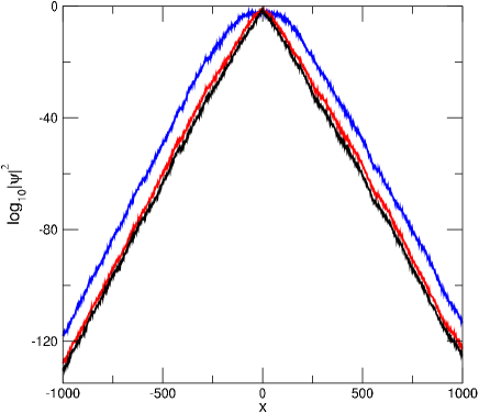
Figure 1: (color online) Probability distribution $\left|\psi\right|^{2}$ over lattice sites $x$ for $J=1$, $w=4$ and for $\beta=1$, $t=10^{8}$ (top blue/solid curve); $t=10^{5}$ (middle red/grey curve); $\beta=0$, $t=10^{5}$ (bottom black curve). (Fig. 2 of [8]).

It consists of a relatively flat region at the center and exponentially decaying tails. The theory of [12, 10] assumes spreading from the relatively flat region of the wavepacket to the region where the amplitude of the wavepacket is small. Let $m_{1},m_{2}$ and $m_{3}$ designate eigenstates of $H_{0}$ with the centers of localization found within the flat region, and let $n$ designate a state with a center of localization found in the tail of the wavepacket, but in the vicinity of the flat region. Therefore, spreading will take place to the region where the $n$-th state is localized,

$$|c_{m_{1}}|^{2}\approx|c_{m_{2}}|^{2}\approx|c_{m_{3}}|^{2}\approx\rho$$ (13)

while

$$|c_{n}|^{2}\ll\rho.$$ (14)

It is further assumed that the RHS of (11) is a random function denoted by $F_{n}\left(t\right)$, of the form [12],

$$F_{n}=C_{1}P\beta\rho^{3/2}f_{n}(t)$$ (15)

where

$$P=C_{2}\beta\rho.$$ (16)

Equation (16) is the probability of a “resonance” between four modes, $C_{1}$ and $C_{2}$ are constants, while $f_{n}\left(t\right)$ is a random function with a rapidly decaying correlation function, $C\left(t\right)$. Introduction of $P$ and the assumption that it satisfies (16), in particular its linearity in $\beta$, are the strongest assumptions of the theory, which still require justification. In [12] it is claimed that numerical calculations support this assumption. Under these assumptions (11) reduces to

$$i\partial_{t}c_{n}(t)=F_{n}(t).$$ (17)

Assuming that $F_{n}(t)$ can be considered random, with rapidly decaying correlations in time, integration results in

$$c_{n}(t)=-iC_{1}P\beta\rho^{3/2}\int^{t}dt^{\prime}f_{n}(t^{\prime}).$$ (18)

Averaging over realizations one finds

$$\left\langle\left|c_{n}\right|^{2}\right\rangle=C_{3}\beta^{4}\rho^{5}t,$$ (19)

where

$$C_{3}=C_{1}C_{2}\int_{0}^{\infty}C\left(t^{\prime}\right)\,\mathrm{d}t^{\prime}.$$ (20)

The equilibration time, $T$, is the time when $\left\langle\left|c_{n}\right|^{2}\right\rangle\approx\rho$ ,

$$T\propto\frac{1}{\beta^{4}\rho^{4}}.$$ (21)

During the time, $T$, the flat region spreads so that it covers the site where the state $n$ was localized. The resulting diffusion coefficient satisfies,

$$D\propto\frac{1}{T}\propto\beta^{4}\rho^{4}.$$ (22)

At time scales $t\gg T$, diffusion takes place and

$$\frac{1}{\rho^{2}}\propto M_{2}\propto Dt\propto\beta^{4}\rho^{4}t$$ (23)

Where $M_{1}=\sum x\left|\psi\left(x,t\right)\right|^{2}$ is the first moment and

$$M_{2}=\sum_{x}\left(x-M_{1}\right)^{2}\left|\psi\left(x,t\right)\right|^{2}$$ (24)

is the second moment. Therefore,

$$\frac{1}{\rho^{2}}\propto\left(\beta^{4}t\right)^{1/3},$$ (25)

and the second moment satisfies,

$$M_{2}\propto\beta^{4/3}t^{1/3}.$$ (26)

In agreement with the numerical results presented in Fig. 2.

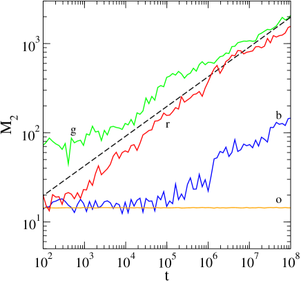
Figure 2: (color online) $M_{2}$ versus time in log-log plots. For $J=1$, $w=4$ and $\beta=0,0.1,1,4.5$ ((o)range, (b)lue, (g)reen, (r)ed). The disorder realization is kept unchanged. The dashed straight line guides the eye for exponent 1/3 (Fig. 2 of [12]).

The equilibration time satisfies,

$$T\propto\beta^{-4/3}t^{2/3}.$$ (27)

Therefore the theory is consistent, as $T\ll t$ for large $t$.

The crucial assumption of the theory presented in this section is that $F_{n}\left(t\right)$ behaves as noise with a rapidly decaying correlation function so that the integral (20) converges. This assumption was explicitly tested [52]. The reasons for $F_{n}\left(t\right)$ to behave as a random variable is that the sum (11) consists of many terms with random phases, and the dynamics of the $c_{n}\left(t\right)$ are chaotic, since these are generated by the nonlinear Hamitonian, $H_{NLS}$.

A crossover to the regime (26) from the regime where a different power law is found is presented in [53].

2.2 Scaling

The theory presented in the previous subsection assumes that $F_{n}\left(t\right)$ is effectively random inside the relatively flat region of the wavepacket. Chaotic behavior of the $\psi\left(x\right)$ would generate such an $F_{n}$. As time evolves, the width of this region increases, and the density, $\rho$, decreases. The first is expected to enhance chaos, and the second to suppress it. The calculation of the present subsection [54] was performed in order to check which effect wins. Since one is limited in the length of the system one can study numerically, the calculation is performed for a system that is finite but its behavior was found not to change as the size of the system is increased. Therefore, it can be extrapolated to arbitrarily large system sizes. In particular, the probability for a system to be regular as a function of its length, $L$, density, $\rho$ and the distribution of the random potential, $w$, was studied. A system is considered regular, if all its Lyapunov exponents vanish, and it is considered chaotic, if at least one Lyapunov exponent is positive. In the present subsection a theory for the flat region of Fig. 1 is presented. For this purpose a dynamics generated by (1) for a finite system of size $L$ is examined. The linear system is invariant under the rescaling,

$$J\to J^{\prime}=cJ,\qquad w\to w^{\prime}=cw$$ (28)

if time and energy are correspondingly rescaled. In particular, the localization length is unaffected. For the nonlinear systems also the rescaling of the norm or the nonlinearity coefficient,

$$\beta\to\beta^{\prime}=c\beta,$$ (29)

is required. In the present work the choice

$$c=\frac{1}{J\left(1+W\right)}$$ (30)

was made resulting in,

$$J^{\prime}=\frac{1}{1+W}\qquad w^{\prime}=\frac{w}{J\left(1+W\right)}\qquad\beta^{\prime}=\frac{\beta}{J\left(1+W\right)}.$$ (31)

In particular we may choose $J=1$, and $W=w/2$ and study the model (1) with $J$ replaced by $J^{\prime}=1/\left(1+W\right)$ the random potential satisfies,

$$-\frac{W}{1+W}\leq\varepsilon_{x}\leq\frac{W}{1+W}$$ (32)

and $\beta$ replaced by $\beta^{\prime}=\beta/\left(1+W\right)$. For convenience this factor can be absorbed in the definition of the norm of the wavefunction,

$$\mathcal{N}^{\prime}=\frac{\beta\mathcal{N}}{1+W}.$$ (33)

The density is,

$$\rho=\frac{\mathcal{N}^{\prime}}{L}.$$ (34)

It was found that for the fixed $W$ and $\rho$, the probability to observe regularity decreases with the length $L$. This behavior can be understood as follows. Suppose we fix $W,\rho$ and consider a lattice of large length $L$. One divides this lattice into (still large) subsystems of lengths $L_{0}$. How the probability to observe regularity on the large lattice $P(\rho,W,L)$ is related to the corresponding probabilities for smaller lattices $P(\rho,W,L_{0})$? It is reasonable to assume that to observe regularity in the whole lattice all the subsystems have to be regular, because any chaotic subsystem will destroy regularity. This immediately leads the relation

$$P(\rho,W,L)=[P(\rho,W,L_{0})]^{L/L_{0}}\;.$$ (35)

Equation (35) implicitly assumes that chaos appears not due to an interaction between the subsystems, but in each subsystem (of length $L_{0}$) separately. This appears reasonable if the interaction between the subsystems is small, i.e. if their lengths are large compared to the length scale associated with localization in the linear problem: $L_{0}\gg\xi$ ($\xi$ is the localization length). On these scales the various subsystems are statistically independent. This is the content of (35). It motivates the definition of the $L$- independent quantity,

$$R(\rho,W)=[P(\rho,W,L)]^{1/L}\;.$$ (36)

This scaling relation was verified numerically, starting with a uniform distribution and using periodic boundary conditions. It was found that for lattices of sizes $16<L<128$, $R$ is independent of $L$. Therefore, to calculate $P$ it is sufficient to evaluate,

$$P_{0}\left(\rho,W\right)\equiv P(\rho,W,L_{0}),$$ (37)

for a system of some size $L_{0}$. It is assumed that the scaling found, will hold for systems of arbitrarily large size, which allows to increase also the localization length. It is convenient to perform a transformation to a new quantity $Q(\rho,W)$ as $Q=P_{0}/\left(1-P_{0}\right)$, which yields,

$$P_{0}=\frac{1}{1+Q^{-1}(\rho,W)}.$$ (38)

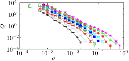
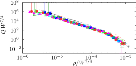
Figure 3: (Color online) The function $Q(\rho,W)$ (top) and the same function in scaled coordinates (bottom). The black dashed and red dotted lines, are showing asymptotics for small and large arguments of $q$, have slopes $\zeta=9/4$ and $\eta=5.2$. (Fig. 4 and 5 of [54])

The limits $\rho\to 0$ (linear problem) and $W\to 0$ (non-random system) are singular, therefore it is expected and indeed observed that the function $Q(\rho,W)$ is not an arbitrary function of $\rho$ and $W$, but it can be written in a scaling form

$$Q=\frac{1}{W^{\alpha}}q\left(\frac{\rho}{W^{\alpha_{1}}}\right),$$ (39)

where $q(x)$ is a singular function at its limits, $q(x)\sim c_{1}x^{-\zeta}$ for small $x$, while $q(x)\sim c_{2}x^{-\eta}$ for large $x$. The top of Fig. 3 collapses to one curve as shown in the bottom of Fig. 3. This is the numerical justification for (39). It also provides the values of the exponents $\alpha=\alpha_{1}\approx 1.75$, $\zeta\approx 9/4=2.25$, $\eta\approx 5.2$, $c_{1}\approx 2.5\cdot 10^{-7}$ and $c_{2}\approx 1.8\cdot 10^{-18}$.

In particular, for a fixed density, $P_{ch}\sim\rho^{9/4}$, since the probability of chaos is fixed and non-zero, spreading is expected. In this aspect model (1) differs from the corresponding $N-$body problem, where for a fixed density and in the thermodynamic limit, localization was found [35, 36]. Now let us assume that we consider the states with the same fixed norm $\mathcal{N}$ on lattices of different length $L$. Then, $\rho=\mathcal{N}/L$, and one finds

$$P_{ch}\approx\frac{L^{1-\zeta}\mathcal{N}^{\zeta}W^{\alpha(1-\zeta)}}{c_{1}L_{0}}=\frac{L^{-5/4}\mathcal{N}^{9/4}}{c_{1}L_{0}W^{35/16}}.$$ (40)

This quantity, as expected, grows with the norm $\mathcal{N}$ and decreases with the disorder $W$. We see that because $\zeta>1$, the probability to observe chaos in large lattices at fixed norm tends to zero. This result may have implications for the problem of spreading of an initially localized wave packet in large lattices. In this setup the norm of the field is conserved, and the effective density decreases in the course of the spreading. This means that as a function of time $L$ increases and $P_{ch}$ decreases, therefore, spreading takes place for less and less realizations of the disorder.

2.3 Study of the relation to phase-space structures

It is expected that in the course of spreading, as the nonlinearity decreases, the trajectories in the $\psi\left(x\right)$, $\psi^{*}\left(x\right)$ phase-space will become more and more regular. In particular, trajectories that look chaotic on some scale may eventually look regular. For this purpose the technique of the time-dependent Lyapunov exponents was introduced [55]. It suggests that an initially chaotic wavepacket may stick to KAM like trajectories resulting in a slow-down of the spreading. A mechanism for spreading that involved a resonance of three oscillators resulting in a mechanism for Arnold diffusion was recently proposed [56]. It is a spot in phase-space where the local Lyapunov exponents are positive and there is wandering in phase-space, presumably, in the regions where tori are destroyed.

A recent qualitative argument for a finite probability for spreading, combined with numerical results was presented [57]. It is instructive to compare it with rigorous statements on the same model [49].

2.4 The renormalized perturbation theory

Since there is no spectral theory for nonlinear equations analysis in the framework of the time dependent perturbation theory was performed [58, 13, 14]. The objective is to develop a perturbation expansion of the $c_{m}\left(t\right)$ of (11) in powers of $\beta$ and to calculate them order by order in $\beta.$ The required expansion is

$$c_{n}\left(t\right)=c_{n}^{\left(0\right)}+\beta c_{n}^{\left(1\right)}+\beta^{2}c_{n}^{\left(2\right)}+\cdots+\beta^{N}c_{n}^{\left(N\right)}+Q_{n},$$ (41)

where the expansion is till order $N$ and $Q_{n}$ is the remainder term (clearly, $c_{n}^{\left(l\right)}$ and $Q_{n}$ are random variables). The initial condition

$$c_{n}\left(t=0\right)=\delta_{n0},$$ (42)

was assumed. The equations for the two leading orders are presented in what follows. The leading order is

$$c_{n}^{\left(0\right)}=\delta_{n0}.$$ (43)

And the first order is

$$c_{n}^{\left(1\right)}=V_{n}^{000}\left(\frac{1-e^{i\left(E_{n}-E_{0}\right)t}}{E_{n}-E_{0}}\right).$$ (44)

The divergence of this expansion for any value of $\beta$ may result from three major problems: the secular terms problem, the entropy problem (i.e., factorial proliferation of terms), and the small denominators problem. To eliminate the secular terms the ansatz (10) is replaced by [13]

$$\psi\left(x,t\right)={\displaystyle\sum\limits_{n}}c_{n}\left(t\right)e^{-iE_{n}^{\prime}t}u_{n}\left(x\right),$$ (45)

where

$$E_{n}^{\prime}\equiv E_{n}^{\left(0\right)}+\beta E_{n}^{\left(1\right)}+\beta^{2}E_{n}^{\left(2\right)}+\cdots$$ (46)

and $E_{n}^{\left(0\right)}$ are the eigenvalues of $H_{0}$ (clearly, $E_{n}^{\left(l\right)}$, are random variables), and $E_{n}^{\prime}$ are the renormalized energies. The new equation for the $c_{n}$ is given by

$$i\partial_{t}c_{n} = \left(E_{n}^{\left(0\right)}-E_{n}^{\prime}\right)c_{n}$$

$$+ \beta\sum_{m_{1}m_{2}m_{3}}V_{n}^{m_{1}m_{2}m_{3}}c_{m_{1}}^{\ast}c_{m_{2}}c_{m_{3}}e^{i\left(E_{n}^{\prime}+E_{m_{1}}^{\prime}-E_{m_{2}}^{\prime}-E_{m_{3}}^{\prime}\right)t}.$$

Inserting expansions (41) and (46) into (2.4) and comparing the powers of $\beta$ without expanding the exponent in $\beta$, produces the following equation for the $k-th$ order

$$i\partial_{t}c_{n}^{\left(k\right)} = -\sum_{s=0}^{k-1}E_{n}^{\left(k-s\right)}c_{n}^{\left(s\right)}+$$

$$+ \sum_{m_{1}m_{2}m_{3}}V_{n}^{m_{1}m_{2}m_{3}}\left[\sum_{r=0}^{k-1}\sum_{s=0}^{k-1-r}\sum_{l=0}^{k-1-r-s}c_{m_{1}}^{\left(r\right)\ast}c_{m_{2}}^{\left(s\right)}c_{m_{3}}^{\left(l\right)}\right]e^{i\left(E_{n}^{\prime}+E_{m_{1}}^{\prime}-E_{m_{2}}^{\prime}-E_{m_{3}}^{\prime}\right)t}.$$

The relation to the order by order expansion in powers of $\beta$ was presented in [14].

The perturbative approach gives an explicit value of the wavepacket for long times, with a rigorous control of the error (Fig. 4). In particular, it rules out spreading for the NLSE with $J=1$, $w=4$, $\beta=0.1$ for time of order $t=10^{5}$ [59].

2.4.1 The remainder of the expansion

In order to control the solution one has to control, $Q_{n}$, the remainder of the expansion (41) that can be written in the form

$$c_{n}\left(t\right)=\tilde{c}_{n}+Q_{n},$$ (49)

with

$$\tilde{c}_{n} = \sum_{l=0}^{N}\beta^{l}c_{n}^{\left(l\right)}.$$ (50)

The linear part of the full equation for the remainder is given by

$$i\partial_{t}\tilde{Q}_{n}^{lin}=W_{n}\left(t\right)+\sum_{m}M_{nm}\left(t\right)\tilde{Q}_{m}^{lin}+\sum_{m}\bar{M}_{nm}\left(t\right)\left(\tilde{Q}_{m}^{lin}\right)^{*}.$$ (51)

The contribution of the remainder term is

$$\left|Q_{n}\right|\leq\mathrm{const}\cdot e^{6cN^{2}+N\ln\beta+\ln t}e^{-\gamma\left|x_{n}\right|},$$ (52)

where $\gamma=1/\xi$ is the inverse localization length, $x_{n}$ is the localization center of the $n-$th state. Note that for a given $t$ and $\beta$ there is an optimum $N$ for which the remainder is minimal. Additionally, for any fixed time and order $N$, $\lim_{\beta\rightarrow 0}\left|Q_{n}\right|/\beta^{N-1}=0$ (see definition at [13]), which shows that the series is in fact an asymptotic one [60]. Using a bootstrap argument, one can show [13] that until some time $t_{*}$ , the dynamics is governed by the linear part and the remainder is bounded by,

$$\left|Q_{n}\left(t\right)\right| \leq A\beta^{N}t\cdot e^{-\gamma\left|x_{n}\right|},$$ (53)

where $\gamma$ is the inverse localization length and $A$ is a constant. Therefore to estimate the remainder one can integrate (51) at least up to $t_{*}$. It is useful to integrate up to some large time, $t\ll t_{*},$ and then to extrapolate using the linear bound (53) up to $t_{*}$. In the next subsection it will be proposed how to determine $t_{*}$ in practice.

For time shorter than $t_{*}$ there is a front $\bar{x}\left(t\right)\propto\ln t$ such that for $x_{n}>\bar{x}\left(t\right)$ both the remainder, $Q_{n}\left(t\right)$ and $c_{n}\left(t\right)$ are exponentially small.

2.4.2 Practical estimate of the remainder

In this section it will be demonstrated, how the numerical scheme for calculations in the framework of the perturbation theory, is implemented in practice for a specific realization of the random potentials $\left\{\varepsilon_{x}\right\}$. It was found that there are some modes that result in the largest contributions to the remainder. These modes are located near the initial mode and therefore can be easily identified and subtracted. For numerical evaluations one defines a norm

$$\left\|Q\right\|_{2}\equiv\left(\sum_{m}\left|Q_{m}\right|^{2}\right)^{1/2},$$ (54)

the definition of $\left\|Q_{lin}\right\|_{2}$ is similar. It was found that for $\left\|Q_{lin}\right\|_{2}\leq 0.1$, $\left\|Q_{lin}\right\|_{2}$ is close to $\left\|Q\right\|_{2}$ , which leads to the definition of $t_{*}$,

$$\left\|Q_{lin}\left(t_{*}\right)\right\|_{2}=0.1.$$ (55)

For small nonlinearity strength, $\beta$, $t_{*}$ is very large and therefore the integration of (51) to $t_{*}$ is very time consuming. Equation (55) can be used to extrapolate linearly from the time interval where (51) is solved to $t_{*}$. Practically, one can find $t_{*}$ from (55) by extrapolation. In Fig. 4 a plot of $\log_{10}t_{*}$ as a function of $\beta^{-1}$ for different orders is presented.

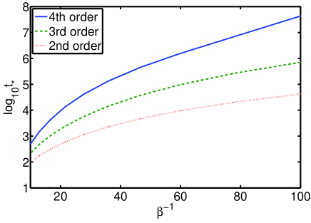
Figure 4: $\log_{10}t_{*}$ as a function of $\beta^{-1}$ for different orders. 4th order (solid blue), 3rd order (dashed green) and 2nd order (dotted red). The parameters are: $w=4$, $J=1$.

A systematic improvement with the order of the perturbation theory is found. Note, that even with moderate nonlinearity strengths, namely, $\beta<0.08$, one can achieve a good approximation of the solution up to very large times. In this way the perturbation theory combined with the solution of the linear equation (51) and the criterion (55) may be used to obtain the solution of the original equation (1) up to $t<t_{*}$. For small $\beta$ the time $t_{*}$ is very long, as is clear from Fig. 4. Removing the dominant modes, which were mentioned in the beginning of this subsection, allows to obtain reliable results for times larger by more than one order of magnitude from the times presented at Fig. 4 (see, Fig. 10 in [14]). When one considers the smallness of $\beta$ one should consider actually the smallness of $\beta e^{2}$ due to the exponential proliferation of the number of terms (see Eq. (4.6) of [13]).

3 Rigorous results

The rigorous analysis of the NLSE equation with a random potential turned out to be very difficult as well. The results so far are very limited in scope, yet of sufficient interest to point out the nature of the problem at hand. Most notably we have the following conclusive results.

3.1 Many body localization

Consider the system of $N$ interacting particles via finite range interactions, on a finite $d-$ dimensional lattice, $\mathbb{Z}^{d}$, with the Hamiltonian

$$H^{\left(N\right)}\left(\omega\right)=\sum_{j=1}^{N}\left[-\Delta_{j}+\lambda V\left(x_{j};\omega\right)\right]+\sum_{i<j}V_{ij}\left(x_{i}-x_{j}\right)$$ (56)

acting on the Hilbert space $\mathcal{H}^{\left(N\right)}=\ell^{2}\left(\mathbb{Z}^{d}\right)^{N}.$ It is assumed, for simplicity, that the $V_{ij}$ are all uniformly bounded by a constant, $0<\alpha<\infty$, and the random potential $V\left(x_{j};\omega\right)$ is given in terms of a collection of i.i.d random variables, $\left\{V\left(x,\omega\right)\right\}_{x\in\mathbb{Z}^{d}}$, with bounded probability distribution and finite moment generating function

$$\mathbb{E}\left(\exp\left(tV\left(0\right)\right)\right)<\infty\qquad\forall t.$$ (57)

Under the above assumptions on the potentials, it was proved that for a large disorder, the spectrum of $H^{\left(N\right)}$is a dense point spectrum with probability 1, and the eigenfunctions are exponentially localized, after an appropriate distance function is defined on the lattice, between clusters of particles [38, 39]. This important result shows that the inter-particle interactions between, say, electrons in a solid, cannot destroy Anderson localization, at least under some favorable situations. However, this result requires the size of the disorder to be dependent on $N$, the number of particles! Therefore, it cannot be applied to systems with non-zero density of particles, as systems studied in [35, 36].

3.2 Quasi-periodic perturbations

We now turn to the fully nonlinear problem. The first important result in this case is [47], where the time-independent problem was explored. The nonlinear term of the NLSE is considered as a small perturbation of the linear dynamical system corresponding to the linear Anderson problem on the lattice. One is then led to consider the KAM theory in infinite dimensional phase–space, as a way to construct periodic and quasi-periodic solutions (in time) for such models. This has been shown to apply to models with good Diophantine properties (linear combination with integer coefficients, bounded away from zero) of the eigenvalues of the linear part. The possibility that the solutions are localized in space and quasi-periodic in time, notably leads to the question of whether linearizing the NLSE around such a solution, will result in a linear system with localized states only. The idea behind the use of quasi-periodic in time models is that it comes from a formal iterative scheme for solving the NLSE with localized solutions. If a localized solution of the equation is assumed, it can be expanded in terms of the normal modes (eigenfunctions) of the linear problem, so that

$$\psi_{N}\left(x\right)=\sum_{j=1}^{b\left(N\right)}c_{j}u_{j}\left(x\right)e^{-iE_{j}t},$$ (58)

where $N$ is the iteration number, and $b\left(N\right)$ is the number of modes generated by $N$ iterations. In this approximation the nonlinearity is given by,

$$\lambda\left|\psi_{N}\right|^{2}=\lambda\left|\sum_{j=1}^{b\left(N\right)}c_{j}u_{j}\left(x\right)e^{-iE_{j}t}\right|^{2}.$$ (59)

Therefore, the approximate dynamics is governed, to this order by,

$$i\partial_{t}\psi=\left(-\Delta+V\right)\psi+\lambda\left|\psi_{N}\right|^{2}\psi.$$ (60)

A uniform (in $N)$ proof of complete dynamical localization, for the linear equation presented above, would imply localization for the NLSE problem. However, in this iteration scheme $b\left(N\right)$ grows very fast in $N$, and furthermore, the frequencies in $\lambda\left|\psi_{N}\right|^{2}$ may be of an arbitrarily small value, which is hard to control [61]. This is just another manifestation of the small denominator problem one encounters in other perturbative methods.

This approach was followed in a series of papers, beginning with [62], where the Anderson model on a lattice is perturbed by an exponentially localized time-periodic potential. It was shown that the corresponding Floquet operator has purely dense point spectrum, with exponentially localized eigenfunctions. This implies, by general spectral theory that the original equation has dynamical localization, namely, the initial solution does not spread. This was further generalized to the much harder case of exponentially localized, quasi-periodic in time potential perturbations of the Anderson model on the lattice with a similar result - complete localization for small potential perturbations [61]. The key estimates can be formulated as localization for the Floquet operator of the type (for two non-commensurate frequencies)

$$K\equiv-i\omega_{1}\frac{\partial}{\partial\theta_{1}}-i\omega_{2}\frac{\partial}{\partial\theta_{2}}+\epsilon\Delta+V+W_{1}\left(j\right)\cos 2\pi\theta_{1}+W_{2}\left(j\right)\cos 2\pi\theta_{2},$$ (61)

acting on the Hilbert space $H_{K}\equiv\ell^{2}\left(\mathbb{Z}^{d}\right)\otimes L^{2}\left(\mathrm{T}^{2}\right)$ (here, $\mathrm{T}^{2}$ stands for a two-dimensional torus). Then localization was proved with large probability, and for a corresponding set of Diophantine conditions needed in the quasi-periodic case [62, 61]. In particular, it was shown that with large probability, $K$ has a dense point spectrum, with exponentially decaying eigenfunctions. However, the estimates deteriorate as the quasi-periodic frequencies approach zero, which makes them hard to use for the solution of the full NLSE problem.

Further results on models approximating in various ways the NLSE problem, include [42], where it is shown that quasi-periodic solutions in time exist, and that they bifurcate from the corresponding quasi-periodic solutions of the linear equation. Another result is that if the nonlinearity coupling constant vanishes at space infinity (at some polynomial rate), then the NLSE with Anderson potential on the lattice has only localized solutions for large disorder [7].

3.3 NLSE with a random potential

Turning our attention to the full NLSE with a random potential problem, very little is known. The most important result, which indicates localization for large times with large disorder and small nonlinearity is in the work of [9]. The main result can be formulated as follows. The small parameter in the problem is $\epsilon=J+\beta$, and $w=1$. Therefore, small $\epsilon$ implies strong disorder $\left(J\ll 1\right)$ and weak nonlinearity $\left(\beta\ll 1\right)$. For an initial data in $\ell^{2},$ localized at the origin, in the sense that,

$$\sum_{\left|j\right|>R}\left|\psi\left(j,t=0\right)\right|^{2}\leq\delta\ll 1,$$ (62)

it was proven[9], that for all $A$ and $\delta>0$ there exists a constant $C\left(A\right)>0,$ $\epsilon\left(A\right)>0$ and $K\left(A\right)>A^{2}$ such that for all $t\leq\left(\delta/C\right)\epsilon^{-A}$ ,

$$\sum_{\left|j\right|>R+K}\left|\psi\left(j,t\right)\right|^{2}\leq 2\delta,$$ (63)

with probability

$$1-\exp\left(-\frac{R}{K}e^{-2K_{\epsilon}^{1/CA}}\right),$$ (64)

for all $0<\epsilon<\epsilon\left(A\right)$. In this context, it should be noted that the methods used to prove such results, follow the infinite dimensional generalization of dynamical systems theory. It includes a construction of normal form transformations to approximately “diagonalize” the system. Such methods were used already in [49] to prove a similar result for the nonlinearly coupled random masses. This result implies that the $\ell^{2}-$norm grows at most logarithmically in time [9]. However, it is hard to compare these estimates to other results, since the constants are not controlled in this analysis. Note, that the corresponding results (52) and (53) of the perturbation theory are for arbitrary strength of disorder, and improve when it increases.

Another class of results, which give explicit estimates on the solution of NLSE with a random potential was developed in [58, 13, 14]. One can construct renormalized time-dependent perturbation theory for the solutions, starting from the eigenfunctions of the linear problem as a basis. It is then shown, that after eliminating the secular terms, we get an explicit expansion, which is computable. Each term depends explicitly on the potential of the linear problem and the eigenvalues. Therefore, by using the known and some new results on the linear spectral problem it is possible to estimate the various terms in the expansion on average. In particular, in [63] it is shown that for the linear problem in one dimension, if the potentials are uniformly bounded by some finite constant, then for all potentials the minimal distance between the eigenvalues is nonzero, bounded below by $e^{-cN}$, where $N$ is the size of the lattice. This is then used to control rigorously the first order term in the above expansion (41),(44), and to conclude that to this order the exponential localization persists in the nonlinear case. It should be noted that the lower bound on the distance between the eigenvalues, though exponentially small, is sufficient to the purpose of controlling the various terms in the renormalized expansion. It also allows to obtain bounds without the usual Diophantine conditions. Moreover, it implies a bound on the expectation of the derivative of the eigenfunctions with respect to the potential,

$$\sum_{i=1}^{N}\mathbb{E}\left|\frac{\partial\psi_{i}\left(x\right)}{\partial\varepsilon_{j}}\right|\leq CN.$$ (65)

However, to control the higher order terms in the expansion, a control of linear combinations of more than two eigenvalues is needed. In the work of [34] there are Diophantine estimates on the eigenvalues of the linear problem that can similarly control many other terms in the expansion of [58, 13, 14]. However, this is not sufficient for complete control in the probabilistic sense of the linear combinations of the eigenvalues of the linear problem, to bound all the terms in the expansion.

4 Numerical results

The main problem one encounters with the numerical calculation for chaotic systems is the exponential sensitivity to numerical errors. For this reason one cannot perform the calculation for substantially long time scale with a control on the errors of a specific solution. The validity of the results is traditionally tested by changing the size of the steps verifying that the results are not affected. The correct result is assumed to be the one that is found in the limit of a vanishing step size. The main problem with such assumptions is that the limit of zero time step may be singular. Moreover, there is no theoretical understanding that the numerical solutions are some types of sampling of the phase-space as is the situation for chaotic systems. Typically, one finds that after some time, spreading starts, as shown in Fig. 2. Eventually, it turns into a sub-diffusion and the second moment grows according to (26) with the exponent $\nicefrac{{1}}{{3}}$ [10, 11, 12, 64, 65]. The wavepacket is typically of the shape presented in Fig. 1. A theory similar to the one presented in Subsection 2.1 but with the nonlinear term (4) was developed and was found to agree with the numerical results [8, 12, 10, 18, 66]. The longest time for which numerical calculations were performed is $t=10^{8}$ (in units where $J=1$ in (1)).

In order to follow the dynamics of a wavepacket, typically the SABA algorithm is used. This algorithm belongs to the family of split step algorithms and evaluates the wave packet in small steps, changing from coordinate space to momentum space. The disorder and nonlinear interaction are applied in the coordinate space, the wave is then transformed to the momentum space, where the kinetic energy term is applied. The solution in real space is recovered by transforming it back to the coordinate space, and the procedure is repeated. Nearly all numerical calculations for this problem use such methods. Additional details on the SABA algorithm, can be found in [12]. Like any numerical algorithm, the SABA algorithm accumulates errors during the calculation which grow with the time of the integration. There is no reliable estimate of these errors.

Double humped states were studied numerically in the presence of nonlinearity that is not too strong. It was found that the spreading of a wave packet prepared initially near some site $O$ is substantially stronger if there is a double humped state with one of its humps near $O$, than if the states peaked near $O$ are single humped. It was found [67] that there is a regime of parameters where $\beta$ is sufficiently small so that the double humped structure is preserved but the packet is not only oscillating between the humps but also leaks to other states, leading to spreading. Additionally, if $\beta$ is small enough so that the oscillations between the two states are not suppressed in the double-well model, then the double humped states will contribute to the spreading for the NLSE. But since double humped states are suppressed and do not contribute to the spreading for high nonlinearities, it cannot be claimed that they dominate the spreading for the NLSE.

5 Discussion and open problems

All numerical calculations exhibit spreading of an initially localized wavepacket (although some part of it may not spread). The spreading results in sub-diffusion with the exponent $\nicefrac{{1}}{{3}}$. All rigorous and analytical theories predict that asymptotically the spreading cannot be faster than logarithmic in time. The main difficulty is, that there is no regime of parameters, where analytical and numerical results agree for a long time. For short times $\left(t\leq 10^{4}\right)$, perturbation theory was found to agree with the numerical results (and for $t\leq 10^{5}$ in [59]).

5.1 List of open problems

We list the questions that may be explored by the various communities:

1. What is the asymptotic time scale? Namely, what is the time scale where the theories predicting suppression of sub-diffusion become effective.

2. When does spreading start and how this time depends on parameters?

3. Is it possible to analytically derive the scaling theory presented in Subsection 2.2?

4. Can one prove the bound of the terms of the perturbation theory presented in Subsection 2.4? In this theory it is difficult to control denominators of the form $f_{l}=\sum_{i=1}^{l}c_{i}E_{i}$ where $E_{i}$ are the eigenvalues of the Anderson Hamiltonian, $H_{0}$, and $c_{i}$ are integer constants. Numerical calculations show that these satisfy a central limit theorem. In particular, one would like to prove that,

   $$\left\langle\frac{1}{\left|f_{l}\right|^{s}}\right\rangle<\infty\qquad\text{for }0<s<1.$$ (66)

5. Is the system chaotic? Namely, is there an exponential instability of the motion in the $\psi\left(x\right)$, $\psi^{*}\left(x\right)$ phase-space? This is a fundamental question since this phase-space is of infinite dimension.

6. Are there KAM tori? Is there sticking to these tori and is it stable to the numerical errors?

7. Can one design experiments that can be extended to the asymptotic long time regime?

8. May the control of the numerical scheme be improved?

9. Another possible mechanism for spreading is tunneling to exponentially large distances with exponentially small probability in space and time. This cannot be decided using numerical calculations, since only relatively small systems are accessible. Another method should be developed to resolve this issue.

References

References

- [1] P. W. Anderson. Absence of diffusion in certain random lattices. Phys. Rev., 109(5):1492, 1958.
- [2] K. Ishii. Localization of eigenstates and transport phenomena in one-dimensional disordered system. Suppl. Prog, Theor. Phys., 53(53):77–138, 1973.
- [3] E. Abrahams, P. W. Anderson, D. C. Licciardello, and T. V. Ramakrishnan. Scaling theory of localization - absence of quantum diffusion in 2 dimensions. Phys. Rev. Lett., 42(10):673–676, 1979.
- [4] P. A. Lee and T. V. Ramakrishnan. Disordered electronic systems. Rev. Mod. Phys., 57(2):287–337, 1985.
- [5] I. M. Lifshits, L. A. Pastur, and S. A. Gredeskul. Introduction to the theory of disordered systems. Wiley, New York, 1988.
- [6] C. Sulem and P. L. Sulem. The nonlinear Schrödinger equation self-focusing and wave collapse. Springer, 1999.
- [7] J. Bourgain and W. -M. Wang. Diffusion bound for a Schrödinger equation. In Mathematical aspects of nonlinear dispersive equations. Princeton University Press, 2007.
- [8] A. S. Pikovsky and D. L. Shepelyansky. Destruction of Anderson localization by a weak nonlinearity. Phys. Rev. Lett., 100(9):094101, 2008.
- [9] W.-M. Wang and Z. Zhang. Long time Anderson localization for nonlinear random Schrödinger equation. J. Stat. Phys., 134:953, 2009.
- [10] S. Flach, D. Krimer, and Ch. Skokos. Universal spreading of wavepackets in disordered nonlinear systems. Phys. Rev. Lett., 102:024101, 2009.
- [11] S. Flach, D. O. Krimer, and Ch. Skokos. Erratum: Universal spreading of wave packets in disordered nonlinear systems [Phys. Rev. Lett. 102, 024101 (2009)]. Phys. Rev. Lett., 102(20):209903, May 2009.
- [12] C. Skokos, D.O. Krimer, Komineas, and S. S. Flach. Delocalization of wave packets in disordered nonlinear chains. Phys. Rev. E, 79:056211, 2009.
- [13] S. Fishman, Y. Krivolapov, and A. Soffer. Perturbation theory for the nonlinear Schrödinger equation with a random potential. Nonlinearity, 22:2861–2887, 2009.
- [14] Y. Krivolapov, S. Fishman, and A. Soffer. A numerical and symbolical approximation of the nonlinear Anderson model. New J. Phy., 12(6):063035, 2010.
- [15] G. P. Berman and F. M. Izrailev. The Fermi-Pasta-Ulam problem: Fifty years of progress. Chaos, 15(1):015104, 2005.
- [16] JC Bronski. Nonlinear wave propagation in a disordered medium. J. Stat. Phys., 92:995–1015, 1998.
- [17] H. Veksler, Y. Krivolapov, and S. Fishman. Spreading for tbe generalized nonlinear Schrödinger equation with disorder. Phys. Rev. E, 80:037201, 2009.
- [18] M. Mulansky. Localization properties of nonlinear disordered lattices. Universität Potsdam, Diploma thesis, 2009. http://nbn-resolving.de/urn:nbn:de:kobv:517-opus-31469.
- [19] G. P. Agrawal. Nonlinear fiber optics, volume 4th. Academic Press, Burlington, MA ; London, 2007.
- [20] N. K. Efremidis, S. Sears, D. N. Christodoulides, J. W. Fleischer, and M. Segev. Discrete solitons in photorefractive optically induced photonic lattices. Phys. Rev. E, 66(4):046602, 2002.
- [21] J. W. Fleischer, T. Carmon, M. Segev, N. K. Efremidis, and D. N. Christodoulides. Observation of discrete solitons in optically induced real time waveguide arrays. Phys. Rev. Lett., 90(2):023902, 2003.
- [22] L.P. Pitaevskii. Zh. Eksp. Theor. Phys., 40:646, 1961.
- [23] E.P. Gross. Structure of a quantized vortex in boson systems. Nuovo Cimento, 20(3):454–477, 1961.
- [24] E. P. Gross. J. Math. Phys., 4:195, 1963.
- [25] F. Dalfovo, S. Giorgini, L. P. Pitaevskii, and S. Stringari. Theory of Bose-Einstein condensation in trapped gases. Rev. Mod. Phys., 71(3):463–512, 1999.
- [26] A. J. Leggett. Bose-Einstein condensation in the alkali gases: Some fundamental concepts. Rev. Mod. Phys., 73(2):307–356, 2001.
- [27] L. P. Pitaevskii and S. Stringari. Bose-Einstein condensation. Clarendon Press, Oxford ; New York, 2003.
- [28] L. Erdös, B. Schlein, and H. T. Yau. Rigorous derivation of the Gross-Pitaevskii equation. Phys. Rev. Lett., 98(4):040404, 2007.
- [29] E. H. Lieb and R. Seiringer. Proof of Bose-Einstein condensation for dilute trapped gases. Phys. Rev. Lett., 88(17):170409, 2002.
- [30] D. Clement, A. F. Varon, M. Hugbart, J. A. Retter, P. Bouyer, L. Sanchez-Palencia, D. M. Gangardt, G. V. Shlyapnikov, and A. Aspect. Suppression of transport of an interacting elongated Bose-Einstein condensate in a random potential. Phys. Rev. Lett., 95(17):170409, 2005.
- [31] J. E. Lye, L. Fallani, M. Modugno, D. S. Wiersma, C. Fort, and M. Inguscio. Bose-Einstein condensate in a random potential. Phys. Rev. Lett., 95(7):070401, 2005.
- [32] D. Clement, A. F. Varon, J. A. Retter, L. Sanchez-Palencia, A. Aspect, and P. Bouyer. Experimental study of the transport of coherent interacting matter-waves in a 1D random potential induced by laser speckle. New J. Phys., 8:165, 2006.
- [33] L. Sanchez-Palencia, D. Clement, P. Lugan, P. Bouyer, G. V. Shlyapnikov, and A. Aspect. Anderson localization of expanding Bose-Einstein condensates in random potentials. Phys. Rev. Lett., 98(21):210401, May 2007.
- [34] M. Aizenman and S. Warzel. On the joint distribution of energy levels of random Schrödinger operators. J. Phys. A, 42:045201, 2009.
- [35] D.M. Basko, I.L. Aleiner, and B.L. Altshuler. Metal-insulator transition in a weakly interacting many-electron system with localized single-particle states. Ann. Phys., 321:1126, 2006.
- [36] D.M. Basko, I.L. Aleiner, and B.L. Altshuler. Possible experimental manifestations of the many-body localization. Phys. Rev. B, 76:052203, 2007.
- [37] I. L. Aleiner, B. L. Altshuler, and G. V. Shlyapnikov. A finite-temperature phase transition for disordered weakly interacting bosons in one dimension. Nature Phys., 6(11):900–904, 2010.
- [38] M. Aizenman and S. Warzel. Localization bounds for multiparticle systems. Commun. Math. Phys., 290(3):903–934, 2009.
- [39] V. Chulaevsky and Y. Suhov. Multi-particle Anderson localisation: Induction on the number of particles. Math. Phys. Anal. Geom., 12(2):117–139, 2009.
- [40] C. Albanese and J. Fröhlich. Periodic-solutions of some infinite-dimensional hamiltonian-systems associated with non-linear partial difference-equations .1. Commun. Math. Phys., 116(3):475–502, 1988.
- [41] C. Albanese and J. Fröhlich. Perturbation-theory for periodic-orbits in a class of infinite dimensional hamiltonian-systems. Commun. Math. Phys., 138(1):193–205, 1991.
- [42] J. Bourgain and W.-M. Wang. Quasi-periodic solutions of nonlinear random Schrödinger equations. J. Eur. Math. Soc., 10(1):1–45, 2008.
- [43] B. Doucot and R. Rammal. Invariant-imbedding approach to localization .2. nonlinear random-media. J. Phys., 48(4):527–545, 1987.
- [44] B. Doucot and R. Rammal. On anderson localization in nonlinear random-media. Europhys. Lett., 3(9):969–974, 1987.
- [45] D. Hennig and GP Tsironis. Wave transmission in nonlinear lattices. Phys. Rep., 307:334–432, 1999.
- [46] T. Paul, P. Schlagheck, P. Leboeuf, and N. Pavloff. Superfluidity versus Anderson localization in a dilute Bose gas. Phys. Rev. Lett., 98(21):210602, 2007.
- [47] J. Fröhlich, T. Spencer, and C. E. Wayne. Localization in disordered, nonlinear dynamic-systems. J. Stat. Phys., 42(3-4):247–274, 1986.
- [48] D. L. Shepelyansky. Delocalization of quantum chaos by weak nonlinearity. Phys. Rev. Lett., 70(12):1787–1790, 1993.
- [49] G. Benettin, J. Fröhlich, and A. Giorgilli. A Nekhoroshev-type theorem for Hamiltonian-systems with infinitely many degrees of freedom. Commun. Math. Phys., 119(1):95–108, 1988.
- [50] G. Kopidakis, S. Komineas, S. Flach, and S. Aubry. Absence of wave packet diffusion in disordered nonlinear systems. Phys. Rev. Lett., 100(8):084103, 2008.
- [51] M. I. Molina. Transport of localized and extended excitations in a nonlinear Anderson model. Phys. Rev. B, 58(19):12547–12550, 1998.
- [52] E. Michaely and S. Fishman. Effective noise theories for the nolinear schrödinger equation. in preparation, 2011.
- [53] S. Flach. Spreading of waves in nonlinear disordered media. Chem. Phys., 375(2-3):548–556, 2010.
- [54] A. Pikovsky and S. Fishman. Scaling properties of weak chaos in nonlinear disordered lattices. Phys. Rev. E, 83(2):025201, 2011.
- [55] M. Johansson, G. Kopidakis, and S. Aubry. KAM tori in 1D random discrete nonlinear Schrödinger model? Europhys. Lett., 91(5):50001, 2010.
- [56] D. M. Basko. Weak chaos in the disordered nonlinear Schrödinger chain: Destruction of Anderson localization by Arnold diffusion. Annal. Phys., 326(7):1577–1655, 2011.
- [57] M. V Ivanchenko, T. V Laptyeva, and S. Flach. Anderson localization or nonlinear waves? a matter of probability. arXiv:1108.0899v1, 2011.
- [58] S. Fishman, Y. Krivolapov, and A. Soffer. On the problem of dynamical localization in the nonlinear Schrödinger equation with a random potential. J. Stat. Phys., 131(5):843–865, 2008.
- [59] G. Fleishon, Y. Krivolapov, S. Fishman, and A. Soffer. Absense of diffusion for long times at the Nonliear Schrödinger Equation with a random potential. in preparation, 2011.
- [60] A. Erdélyi. Asymptotic expansions. Dover, New-York, 1956.
- [61] J. Bourgain and W. M. Wang. Anderson localization for time quasi-periodic random Schrödinger and wave equations. Commun. Math. Phys., 248(3):429–466, 2004.
- [62] A. Soffer and W.-M. Wang. Anderson localization for time periodic random Schrödinger operators. Commun. Partial Differ. Equ., 28(1-2):333–347, 2003.
- [63] A. Rivkind, Y. Krivolapov, S. Fishman, and A. Soffer. Eigenvalue repulsion estimates and some applications for the one-dimensional Anderson model. J. Phys. A: Math. Theor., 44(30):305206, 2011.
- [64] T. V. Laptyeva, J. D. Bodyfelt, D. O. Krimer, Ch. Skokos, and S. Flach. The crossover from strong to weak chaos for nonlinear waves in disordered systems. Europhys. Lett., 91(3):30001, 2010.
- [65] J. D. Bodyfelt, T. V. Laptyeva, Ch. Skokos, D. O. Krimer, and S. Flach. Nonlinear waves in disordered chains: Probing the limits of chaos and spreading. Physi. Rev. E, 84(1):016205, 2011.
- [66] Ch. Skokos and S. Flach. Spreading of wave packets in disordered systems with tunable nonlinearity. Phys. Rev. E, 82(1):016208, 2010.
- [67] H. Veksler, Y. Krivolapov, and S. Fishman. Double humped states in the nonlinear Schrödinger equation with a random potential. Phys. Rev. E, 81:017201, 2010.