Isomorphs in model molecular liquids

Abstract

Isomorphs are curves in the phase diagram along which a number of static and dynamic quantities are invariant in reduced units. A liquid has good isomorphs if and only if it is strongly correlating, i.e., the equilibrium virial/potential energy fluctuations are more than 90% correlated in the NVT ensemble. This paper generalizes isomorphs to liquids composed of rigid molecules and study the isomorphs of two systems of small rigid molecules, the asymmetric dumbbell model and the Lewis$-$Wahnström OTP model. In particular, for both systems we find that the isochoric heat capacity, the excess entropy, the reduced molecular center-of-mass self part of the intermediate scattering function, the reduced molecular center-of-mass radial distribution function to a good approximation are invariant along an isomorph. In agreement with theory, we also find that an instantaneous change of temperature and density from an equilibrated state point to another isomorphic state point leads to no relaxation. The isomorphs of the Lewis$-$Wahnström OTP model were found to be more approximative than those of the asymmetric dumbbell model, which is consistent with the OTP model being less strongly correlating. For both models we find ”master isomorphs”, i.e., isomorphs have identical shape in the virial/potential energy phase diagram.

I Introduction

For supercooled liquids near the glass transition changing slightly the density $\rho$ or temperature $T$ the structural relaxation time $\tau_{\alpha}$ may change several orders of magnitude. In the study of these liquids^{1; 2; 3} it is found that $\tau_{\alpha}$ does not change when $\rho^{\gamma}/T$ is kept constant, where $\gamma$ is a fixed material-specific exponent. This phenomenon is called density scaling and has been established for many liquids, excluding associative liquids such as water³. A related observation is isochronal superposition^{4; 5; 3}, i.e., that supercooled state points with identical $\tau_{\alpha}$ have the same dielectric spectrum. A different and at first sight unrelated concept is Rosenfeld’s excess entropy scaling^{6; 7}. In this procedure a relation is established between hard-to-predict dynamic properties and easier-to-predict thermodynamic quantities, here the excess entropy via a scaling of the dynamics to so-called reduced units. Initially this was observed for model atomic liquids^{6; 7}, but later it was extended to model molecular liquids^{8; 9; 10} and experimental liquids¹¹.

In a recent series of papers^{12; 13; 14; 15; 16} a new class of liquids was identified. These liquids are characterized by having strong correlation in the NVT ensemble between the equilibrium fluctuations of the instantaneous potential energy $U$ and the virial $W$. Recall that the instantaneous energy $E$ and pressure $p$ can be written as a sum of a kinetic part and a configurational part: $E=K+U$ and $pV=Nk_{B}T+W$, respectively. The correlation between $U$ and $W$ is quantified via the linear correlation coefficient $R$ defined as

$$R=\frac{\langle\Delta W\Delta U\rangle}{\sqrt{\langle(\Delta W)^{2}\rangle}\sqrt{\langle(\Delta U)^{2}\rangle}}.$$ (1)

The class of strongly correlating liquids is defined by $R\geq 0.90$¹². An inverse power-law (IPL) system $r^{-n}$ has correlation coefficient R = 1, since $\Delta W=(n/3)\Delta U$, and only IPL systems are perfectly correlating. In the study of strongly correlating liquids it was discovered that they obey Rosenfeld’s excess entropy scaling, isochronal superposition, as well as density scaling. These types of scalings can be explained in the framework of so-called isomorphs (definition follows later).

Model systems that have been identified^{17; 12; 13; 18; 19; 20} to belong to this class of liquids include the standard single-component Lennard-Jones liquid (SCLJ), the Kob-Andersen binary LJ mixture ^{21; 22} (KABLJ), the asymmetric dumbbell model ²⁰, the Lewis-Wahnström $o$-$terphenyl$ model^{23; 24} (OTP), and several others. Strong $WU$ correlation has been experimentally verified for a molecular van der Waals liquid ²⁵ and for supercritical argon¹⁷. The class of strongly correlating liquids is believed to include most or all van der Waals and metallic liquids, whereas covalently, hydrogen-bonding or ionic liquids are not strongly correlating¹². The latter reflects the fact that competing interactions tend to destroy the strong correlation.

An example of strong $WU$-correlation is given in Fig. 1 for the asymmetric dumbbell model²⁰ (details of this model are provided in Sec. III). Figure 1(a) shows the time evolution of the equilibrium fluctuations of $U$ and $W$ normalized to zero mean and unity standard deviation, Fig. 1(b) shows a scatter plot of the corresponding instantaneous values of $U$ and $W$. $U$ and $W$ are clearly strongly correlated in their equilibrium fluctuations.

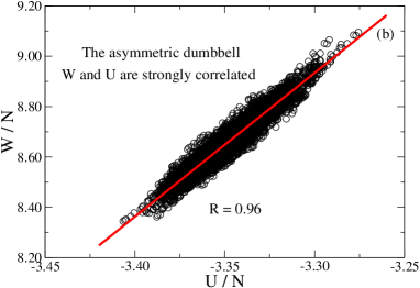
Figure 1: Two different ways of visualizing the strong virial/potential energy correlation for the asymmetric dumbbell model at $\rho$ = $1.863$ and $T$ = $0.465$ (see Sec. III for details of the model and the units used). (a) The time evolution of $U$ (black) and $W$ (red) per particle normalized to zero mean and unity standard deviation. (b) A scatter plot of the instantaneous values of $W$ and $U$ per particle. The correlation coefficient $R$ is $0.96$.

References ¹² and ¹³ identified the cause of strong $WU$-correlation in the SCLJ liquid. The LJ pair potential can be well approximated from about $r=0.95\sigma$ to $r=1.5\sigma$ (see Pedersen et al.²⁶) by a sum of an IPL, a linear term, and a constant via the so-called ”extended IPL potential”¹³: $v_{LJ}(r)\approx Ar^{-n}+B+Cr$. At moderate pressures this covers the entire first peak of the radial distribution function, i.e., the first coordination shell. The constraint of constant volume in the NVT ensemble has the effect that when one nearest neighbor distance increases another one decreases; upon summation the contribution from the linear term to $U$ and $W$ is almost constant. The latter observation has the consequence that some of the scaling properties of pure IPL systems are inherited in the LJ system in the form of isomorphs.

Reference ¹⁵ introduced a new concept referring to a strongly correlating liquid’s phase diagram, namely isomorphic curves or more briefly: isomorphs. Two state points with density and temperature ($\rho_{1}$, $T_{1}$) and ($\rho_{2}$, $T_{2}$) are defined to be isomorphic²⁷ if the following holds: Whenever a configuration of state point ($1$) and one of state point ($2$) have the same reduced coordinates ($\rho_{1}^{1/3}\textbf{r}^{(1)}_{i}=\rho_{2}^{1/3}\textbf{r}^{(2)}_{i}$ for all particles $i$), these two configurations have proportional Boltzmann factors, i.e.,

$$e^{-U(\textbf{r}_{1}^{(1)},...,\textbf{r}_{N}^{(1)})/k_{B}T_{1}}=C_{12}e^{-U(\textbf{r}_{1}^{(2)},...,\textbf{r}_{N}^{(2)})/k_{B}T_{2}}.$$ (2)

Here $C_{12}$ is a constant that depends only on the state points ($1$) and ($2$). An isomorph is defined as a continuous curve of state points that are all pairwise isomorphic. In other words, Eq. (2) defines an equivalence relation with the equivalence classes being the isomorphs. Only IPL systems have exact isomorphs; these are characterized by having $\rho^{\gamma}/T=const$ where $\gamma=n/3$. Reference ¹⁵ argued and demonstrated by simulations that strongly correlating liquids have isomorphs to a good approximation.

From the defining property of an isomorph [Eq. (2)] it follows that the structure in reduced units ($\tilde{\textbf{r}}_{i}\equiv\rho^{1/3}\textbf{r}_{i}$) is invariant along an isomorph, since the proportionality constant $C_{12}$ disappears when normalizing the configurational canonical probabilities¹⁵. Thus the reduced unit radial distribution function and the excess entropy $S_{ex}=S-S_{id}$ are isomorph invariants, where $S_{id}$ is the ideal gas contribution to the entropy at the same temperature and density. Isomorph invariance is, however, not limited to static quantites, also the mean-square displacement, time auto-correlation functions, and higher-order correlation functions are invariant in reduced units along an isomorph. The reader is referred to Ref. ¹⁵ for a detailed description of isomorph invariants, and the proof that a liquid is strongly correlating if and only if it has good isomorphs. A brief overview of strongly correlating liquids and their isomorphs can be found in Pedersen et al²⁶.

Reference ¹⁶ studied isomorphs of atomic single- and multicomponent LJ liquids with generalized exponents $m$ and $n$. It was found that for given exponents ($m$, $n$) all isomorphs have the same shape in the $WU$-phase diagram, i.e., a so-called master isomorph exists from which all isomorphs can be generated via a simple scaling of the $WU$-coordinates. For instance, the shape of isomorphs in the $WU$-phase diagram of the SCLJ liquid and the KABLJ liquid are the same.

References ¹²-¹⁶ focused on understanding strong $WU$-correlation and its implication for atomic systems. Schrøder et al.²⁰ in $2008$ studied two rigid molecular liquids that are strongly correlating: the asymmetric dumbbell model and the Lewis-Wahnström OTP model (see Sec. III). At that time the isomorph concept had not yet been developed and state points with the same $\rho^{\gamma}/T$, as inspired from the IPL system, were tested for collapse of, for instance, the reduced unit radial distribution function (note that in Refs. ¹², ¹³, and ²⁰ $\gamma$ is defined slightly different from subsequent papers). The dynamics in reduced units was also found to be a function of $\rho^{\gamma}/T$, to a good approximation, as is the case for IPL systems¹⁴. Chopra et al. ¹⁰ found that the $S_{ex}$ can be written (approximately) as a function of $\rho^{\gamma}/T$ for rigid symmetric LJ dumbbells with different bond lengths. They also found that the reduced diffusion constant and relaxation time are functions of $S_{ex}$. These results suggest that the isomorph concept is relevant also for rigid molecular systems. In this paper we expand on earlier results by studying in detail the same systems as Schrøder et al.²⁰.

The isomorph definition Eq. (2) must be modified for rigid molecules, since the bond lengths are fixed and cannot follow the overall scaling. A simple modification of Eq. (2), which is consistent with the atomic definition, is to define the mapping amongst configurations in terms of the molecular center of masses, instead of the atomic positions. We thus define two state points in the phase diagram of a liquid composed of rigid molecules to be isomorphic if the following holds: Whenever two configurations of the state points have identical reduced center-of-mass coordinates for all molecules,

$$\rho_{1}^{1/3}\textbf{r}^{(1)}_{CM,i}=\rho_{2}^{1/3}\textbf{r}^{(2)}_{CM,i},$$ (3)

as well as identical Eulerian angles²⁸

$$\theta_{i}^{(1)}=\theta_{i}^{(2)},\ \phi_{i}^{(1)}=\phi_{i}^{(2)},\ \psi_{i}^{(1)}=\psi_{i}^{(2)},$$ (4)

these two configurations have proportional Boltzmann factors, i.e., [where R $\equiv$ ($\textbf{r}_{CM,1}$, $\theta_{1}$, $\phi_{1}$, $\psi_{1}$, …, $\textbf{r}_{CM,N}$, $\theta_{N}$, $\phi_{N}$, $\psi_{N}$)]

$$e^{-U(\textbf{R}^{(1)})/k_{B}T_{1}}=C_{12}e^{-U(\textbf{R}^{(2)})/k_{B}T_{2}}.$$ (5)

Again, $C_{12}$ is a constant that depends only on the state points ($1$) and ($2$). An isomorph is defined as a set of state points that are pairwise isomorphic. It should be noted that, in contrast to what is the case for atomic systems, since the bonds do not follow the overall scaling of the system this definition does not imply the existence of exact isomorphs for rigid molecules with intermolecular IPL interactions,.

Taking the logarithm of Eq. (5) implies

$$U(\textbf{R}^{(2)})=T_{2}/T_{1}\cdot U(\textbf{R}^{(1)})+k_{B}T_{2}\ln\,C_{12}.$$ (6)

Equation (6) provides a convenient way of testing to which extent Eq. (5) is obeyed for a given system. A simulation is performed at one state point ($1$) and the obtained configurations are scaled to a different density $\rho_{2}$, where the potential energy is evaluated. The respective potential energies of the two state points are then plotted against each other. In the resulting plot a near straight-line indicates that there exists an isomorphic state point with density $\rho_{2}$. The temperature $T_{2}$ of the isomorphic state point can be found from the slope of a linear regression fit. This procedure is termed the ”direct isomorph check”¹⁵. If this test is performed for an atomic IPL system a correlation coefficient of $R$ = $1$ is obtained, consistent with these systems having exact isomorphs.

As an example we perform a direct isomorph check for the asymmetric dumbbell model in Fig. 2. A correlation coefficient of $R=0.97$ is observed for a 15% density increase. Calculating the temperature of the isomorphic state point from the linear regression slope the result differs only 1% from the prediction by requiring constant excess entropy (see Sec. IV).

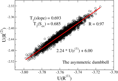
Figure 2: The ”direct isomorph check”¹⁵ for the asymmetric dumbbell model. During a simulation at state point ($\rho_{1}$, $T_{1}$) = (1.737, 0.309) the center of mass of each dumbbell is scaled to density $\rho_{2}$ = 1.998, keeping the Eulerian angles fixed. The potential energy is then evaluated from the scaled configurations and plotted against the potential energy of the unscaled configurations. The temperature $T_{2}$(slope) of the isomorphic state point at density $\rho_{2}$ is calculated by multiplying the linear regression slope with $T_{1}$ [Eq. (6)].

In the present paper we show that liquids composed of simple rigid molecules have good isomorphs in their phase diagram as defined in Eqs. (3) - (5). Section II derives several isomorph invariants in molecular systems composed of rigid molecules. Section III describes the simulation setup and the investigated model systems. Section IV investigates the existence of isomorphs for the asymmetric dumbbell and the Lewis-Wahnström OTP models^{23; 24}. Section V investigates the existence of a master isomorph¹⁶ for these model systems. Section VI summarizes the results and presents an outlook.

II Isomorph invariants in liquids composed of rigid molecules

From the single assumption of curves of isomorphic state points in an atomic liquid’s phase diagram, Ref. ¹⁵ derived several invariants along an isomorph. Since we have extended this definition in Eqs. (3) - (5) to molecular systems composed of rigid molecules, it is natural to wonder which of these invariants can be extended to molecular systems. The molecular isomorph concept is different from the atomic case in that there is no ”ideal” reference system (the IPL system). The following sections and simulations, however, show that isomorphs can nevertheless be a useful tool for understanding such liquids.

In the following we derive several invariants from exact isomorphs. We start by noting that the generalization of isomorphs to molecular systems define a bijective map amongst configurations of state points ($1$) and ($2$). The NVT configurational probability density for a system of $N$ rigid molecules is given by²⁹ (where $d\textbf{R}\equiv d\textbf{r}_{CM}^{N}d\tau^{N}$ with $\tau$ $\equiv$ ($\theta$, $\phi$, $\psi$) and $d\tau=sin\ \theta\ d\theta\,d\phi\,d\psi$)

$$\hat{P}(\textbf{R}) =\frac{e^{-U(\textbf{R})/k_{B}T}}{\int e^{-U(\textbf{R})/k_{B}T}d\textbf{R}}.$$ (7)

In combination with Eq. (5) it follows that all mapped configurations of state points ($1$) and ($2$) have identical Boltzmann probabilities, i.e.,

$$\hat{P}(\textbf{R}^{(1)})d\textbf{R}^{(1)}=\hat{P}(\textbf{R}^{(2)})d\textbf{R}^{(2)}.$$ (8)

For convenience we introduce two configurational distribution functions^{15; 29}

$$P(\textbf{R}) =(V\Omega)^{N}\hat{P}(\textbf{R}),$$ (9)

$$\tilde{P}(\tilde{\textbf{r}}_{CM}^{N},\tau^{N}) =\frac{e^{-U(\rho^{-1/3}\tilde{\textbf{r}}_{CM}^{N},\tau^{N})/k_{B}T}}{\int e^{-U(\rho^{-1/3}\tilde{\textbf{r}}_{CM}^{N},\tau^{N})/k_{B}T}d\tilde{\textbf{r}}_{CM}^{N}d\tau^{N}},$$ (10)

where $\Omega$ is the integral over the Eulerian angles for one molecule ($\Omega=8\pi^{2}$ for a non-linear molecule). $P$ has been introduced to make $\hat{P}$ dimensionless. $\tilde{P}(\tilde{\textbf{r}}_{CM}^{N},\tau^{N})d\tilde{\textbf{r}}_{CM}^{N}d\tau^{N}$ is the probability to observe the system represented by a point in the volume-element $d\tilde{\textbf{r}}_{CM}^{N}d\tau^{N}$ located at $\{\tilde{\textbf{r}}_{CM}^{N},\tau^{N}\}$. $\tilde{P}$ is invariant along an isomorph and is related to $P$ via $\tilde{P}(\tilde{\textbf{r}}_{CM}^{N},\tau^{N})=(N\Omega)^{-N}P(\textbf{R})$ = $\rho^{-N}\hat{P}(\textbf{R})$. We note that the excess entropy $S_{ex}=-(\partial F_{ex}/\partial T)_{N,V}$, where $F_{ex}$ is the excess free energy, can be written as¹⁵

$$S_{ex} =-k_{B}\int(V\Omega)^{-N}P(\textbf{R})\ln P(\textbf{R})d\textbf{R},$$ (11)

$$=-k_{B}\int\tilde{P}\ln\tilde{P}\ d\tilde{\textbf{r}}_{CM}^{N}d\tau^{N}-k_{B}N\ln(N\Omega).$$ (12)

From the above observations we can now derive a number of isomorph invariants in liquids composed of rigid molecules.

1. The molecular center-of-mass structure in reduced units. For a given configuration of the molecular center-of-mass structure in reduced units, all orientations of the molecules of state points ($1$) and ($2$) by Eq. (8) have identical probabilities. The reduced center-of-mass structure is thus invariant along an isomorph.

2. Any normalized distribution function describing the (relative) orientations of molecules with respect to their center-of-mass. All orientations of the molecules with respect to a given molecular center-of-mass configuration of state point ($1$) are mapped to configurations of state point ($2$) with identical probabilities. It thus follows that the normalized distribution function is invariant along an isomorph.

3. The isochoric heat capacity $C_{V}$. The excess heat capacity in the NVT ensemble is given by $C_{V}^{ex}=\langle(\Delta U)^{2}\rangle/k_{B}T^{2}$. Defining $X$ = $U/k_{B}T$ we may write $C_{V}^{ex}=k_{B}\langle(\Delta X)^{2}\rangle$. By Eqs. (6) and (8) it follows that $C_{V}^{ex}$ is invariant along an isomorph, since the constant $k_{B}T_{2}\ln\,C_{12}$ disappears when subtracting the mean. The ideal gas contribution to $C_{V}$ is independent of state point ($C_{V}^{id}=6Nk_{B}/2$ for non-linear molecule).

4. The translational two-body entropy^{30; 31; 10} $S_{t}/N$ = $-\rho k_{B}/2\int[g_{CM}(r)\ln g_{CM}(r)-g_{CM}(r)+1]d\textbf{r}$, where $g_{CM}(r)$ is the radial distribution function for the center of mass of the molecules. The density dependence disappears when switching to reduced units and by Statement 1. the molecular center-of-mass structure in reduced units is invariant along an isomorph, and thus also the radial distribution function (in reduced units).

5. The orientational two-body entropy^{30; 31; 10} $S_{o}/N$ = $-\rho k_{B}/(2\Omega^{2})\int g_{CM}(r)g(\omega^{2}|r)\ln g(\omega^{2}|r)d\omega^{2}d\textbf{r}$, where $\omega^{2}$ denotes a set of angles used to describe the relative orientation of two molecules, and $g(\omega^{2}|r)$ is the conditional distribution function for the relative orientation of two molecules separated by a distance $r$. Applying reduced units this invariant follows from Statements 1. and 2.

6. All $N$-body entropy terms^{30; 31}. The excess entropy can be expanded as $S_{ex}$ = $\sum_{i=1}^{\infty}S_{i}$. The two-body expression $S_{2}=S_{t}+S_{o}$ is given above, where as the higher-order terms are more involved.

7. The excess entropy $S_{ex}$. The excess entropy is given by Eq. (12), and since $\tilde{P}$ is invariant along isomorph, so is the excess entropy. The latter also follows from Statement 6., since each term is invariant.

8. The molecular center-of-mass NVE and Nos$\acute{e}$-Hoover NVT dynamics in reduced units. The reduced dynamics of the atomic positions on account of the constraints is not invariant along an isomorph. Considering instead the molecular center-of-mass motion the constraint force disappears and these equations of motion are invariant along an isomorph in reduced units. The proof is given in Appendix B (a brief summary of constrained dynamics is given in Appendix A).

9. Any average molecular center-of-mass dynamic quantity in reduced units. This follows immediately from Statement 8., since the molecular center-of-mass equations of motion in reduced units are invariant along an isomorph. In particular, this would include a reduced relaxation time $\tilde{\tau}_{\alpha}$.

As detailed above it is necessary to consider the (reduced) center of mass motion and the motion relative to the center of mass separately. Nevertheless, during the investigation of isomorphs we will also consider the reduced atomic quantities to examine their ”invariance”.

An additional consequence of isomorphs is that, since by Eq. (8) two isomorphic state points have identical canonical probabilities, an instantaneous change of temperature and density from an equilibrated state point to another isomorphic state point does not lead to any relaxation. This is called an isomorphic jump¹⁵.

III Simulation details

We studied two model systems of rigid molecules (Fig. 3): the asymmetric dumbbell model ($N$ = 500) and the Lewis-Wahnström OTP model ($N$ = 320).

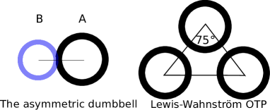
Figure 3: A sketch of the two model systems studied: The asymmetric dumbbell and Lewis-Wahnström OTP models. The asymmetric dumbbell is a simplistic model of toluene with the methyl side-group tightly bonded to the benzene molecule. The Lewis-Wahnström OTP model is an isosceles triangle with an angle of $75^{\circ}$, different from the $60^{\circ}$ of the real 1,2-diphenylbenzene molecule³².

For both models the potential energy $U$ and the virial $W$ are given by

$$U =U_{LJ}$$ (13)

$$W =W_{LJ}+W_{CON}.$$ (14)

The first term in the virial is the LJ virial $W_{LJ}$, the second term is the contribution to the virial due to the constraints (fixed bond lengths), $W_{CON}$. $U_{LJ}$ is a sum over intermolecular pair interactions given by the ($12$, $6$)-LJ potential

$$u(r_{ij})=4\epsilon_{\alpha\beta}\Big{[}\Big{(}\frac{\sigma_{\alpha\beta}}{r_{ij}}\Big{)}^{12}-\Big{(}\frac{\sigma_{\alpha\beta}}{r_{ij}}\Big{)}^{6}\Big{]}.$$ (15)

The potential energy has no contribution from the fixed bonds. A force smoothing procedure³³ was applied from $r_{s}=2.45\sigma_{\alpha\beta}$ to $r_{c}=2.50\sigma_{\alpha\beta}$.

The bond lengths were held fixed using the Time Symmetrical Central Difference (TSCD) algorithm ^{34; 35}, which is a central difference time-discretization of the constrained equations of motion preserving time-reversibility. The simulations were performed in the NVT ensemble applying the Nos$\acute{e}$-Hoover (NH) algorithm^{36; 37; 38} using RUMD³⁹, a molecular dynamics package optimized for state of the art GPU-computing.

The NVT simulations were performed without adjusting the time-constant of the NH algorithm (see Appendix B). This choice is not expected to influence the results over the observed density and temperature range, since the dynamics is not particular sensitive to the absolute value of the NH time-constant⁴⁰.

Appendix A gives a brief summary of constrained dynamics and the effect on the virial (see also Refs. ³⁴, ⁴¹, and ⁴²). The specific details of the investigated two models follow below.

III.1 The asymmetric dumbbell

The asymmetric dumbbell model consists of a big ($A$) and small ($B$) LJ particle, rigidly bonded with bond distance of $r_{ij}=0.584$ (here and henceforth units are given in LJ units referring to the $A$ particle, $\sigma_{AA}$ = 1, $\epsilon_{AA}$ = 1, and $m_{A}$ = 1). The parameters were chosen to roughly mimic Toluene ²⁰. The asymmetric dumbbell model can be cooled to a highly viscous state without crystallizing, making it feasible to study slow dynamics. The asymmetric dumbbell model has $\sigma_{AB}$ = 0.894, $\sigma_{BB}$ = 0.788, $\epsilon_{AB}$ = 0.342, and $\epsilon_{BB}$ = 0.117 with $m_{B}$ = 0.195.

III.2 Lewis-Wahnström OTP

The Lewis-Wahnström OTP model^{23; 24} consists of three identical LJ particles rigidly bonded together in an isosceles triangle with sides of $r_{ij}=1.000$ and top-angle of $75^{\circ}$, i.e., different from the $60^{\circ}$ of the real 1,2-diphenylbenzene molecule³². All parameters (including the masses) are unity for the OTP model.

IV Numerical study of isomorphs for the two model systems

In order to investigate whether the two model systems have good isomorphs, we first describe how to generate an isomorph in a simulation. The excess entropy $S_{ex}$ is invariant along an isomorph, and a method for generating an isomorph is to generate a curve of constant $S_{ex}$ (see Sec. II and also Refs. ¹⁵ and ¹⁶). A curve of constant excess entropy can be found by using the exact NVT ensemble relation¹⁵

$$\frac{\langle\Delta U\Delta W\rangle}{\langle(\Delta U)^{2}\rangle}=\Big{(}\frac{\partial\ln T}{\partial\ln\rho}\Big{)}_{S_{ex}}\equiv\gamma.$$ (16)

In simulations an isomorph is generated as follows: 1) The left-hand side is calculated from the fluctuations at a given state point; 2) A new state point is identified by a dicretization of Eq. (16) by changing the density by 1%, where the new temperature is calculated from $\Delta\ln T=\gamma\Delta\ln\rho$; 3) The procedure is repeated and in this way an isomorph is generated in the phase diagram.

IV.1 Isomorphs of the asymmetric dumbbell model

This section investigates the asymmetric dumbbell model. Isomorphs were mapped out following the procedure described above. Figure 4 shows the $AA$ radial distribution functions along an isomorph with 19% density increase before ($a$) and after ($b$) scaling the distance $r$ into reduced units

$$\tilde{r}=\rho^{1/3}r.$$ (17)

Also shown for reference in Fig. 4(c) is the $AA$ radial distribution functions along an isotherm with 12% density increase. Although the reduced structure of the atomic positions is not predicted to be invariant along an isomorph, Fig. 4 shows that it nevertheless is a resonable approximation. The reduced structure of the atomic positions is less invariant along the isotherm.

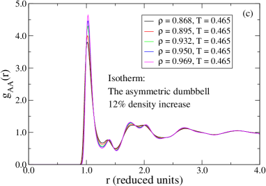
Figure 4: Radial distribution functions for the asymmetric dumbbell model. (a) $AA$ pair-correlation function along an isomorph with 19% density increase before scaling the distance $r$ into reduced units $\tilde{r}=\rho^{1/3}r$. (b) $AA$ pair-correlation function along the same isomorph after scaling the distance $r$ into reduced units. (c) $AA$ pair-correlation function along an isotherm with $12\%$ density increase function after scaling of the distance.

Figure 5 considers the $AB$ radial distribution functions, where the constrained bond distance shows up as a sharp peak. The analogous conclusion as with the $AA$ distribution functions is reached, and likewise for the $BB$ distribution functions (not shown).

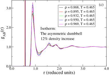
Figure 5: Radial distribution functions for the asymmetric dumbbell model. (a) $AB$ pair-correlation function along the isomorph of Fig. 4 before scaling the distance $r$ into reduced units $\tilde{r}=\rho^{1/3}r$. (b) $AB$ pair-correlation function along the same isomorph after scaling the distance $r$ into reduced units. (c) $AB$ pair-correlation function along the isotherm of Fig. 4 after scaling of the distance.

Next, we consider in Fig. 6 the molecular center-of-mass radial distribution functions along the isomorph and isotherm of Figs. 4-5. This quantity is predicted to be invariant along an isomorph (see Sec. II). The molecular center-of-mass structure is to a good approximation invariant in reduced units along the isomorph, while this is less so along the isotherm as can be seen from the first peak.

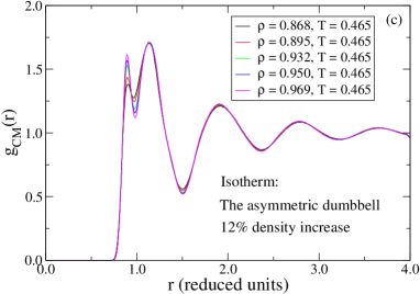
Figure 6: Molecular center-of-mass radial distribution functions for the asymmetric dumbbell model. (a) Pair-correlation function along the isomorph of Figs. 4-5 before scaling the distance $r$ into reduced units $\tilde{r}=\rho^{1/3}r$. (b) Pair-correlation function along the same isomorph after scaling the distance $r$ into reduced units. (c) Pair-correlation function along the isotherm of Figs. 4-5 after scaling of the distance.

We consider in Fig. 7 the dynamics in terms of the reduced $A$-particle incoherent intermediate scattering function. The reduced dynamics of the atoms is not predicted to be invariant along an isomorph (see Appendix B), however, the figure shows that it is a good approximation. The same conclusion is reached for the $B$-particle (not shown).

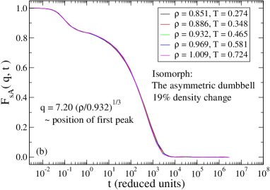
Figure 7: The reduced $A$-particle incoherent intermediate scattering function for the asymmetric dumbbell model keeping the reduced wavevector $q$ constant. (a) Along the isotherm of Figs. 4-6 with 12% density increase. (b) Along the isomorph of Figs. 4-6 with 19% density increase.

In Figure 8 we consider the reduced molecular center-of-mass self part of the intermediate scattering function. This quantity is predicted to be invariant along an isomorph (see Appendix B), and Fig. 8 clearly shows this. The dynamics is not invariant along the isotherm.

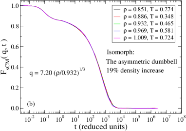
Figure 8: The reduced molecular center-of-mass incoherent intermediate scattering function for the asymmetric dumbbell model keeping the reduced wavevector $q$ constant. (a) Along the isotherm of Figs. 4-7 with 12% density increase. (b) Along the isomorph of Figs. 4-7 with 19% density increase.

We show the variation of $\gamma$, calculated from the NVT fluctuations via Eq. (16), in Fig. 9 along an isochore and along the isomorph of Figs. 4-8 in two different versions. The crosses show $\gamma$ calculated from the total virial $W$ while the asterisks show $\gamma$ calculated after subtracting the constraint contribution to virial, i.e., replacing $W$ with $W_{LJ}=W-W_{CON}$. The insets show the corresponding correlation coefficients $R$. Reference ¹⁵ predicts that $\gamma$ should be a function of density only $\gamma$ = $\gamma(\rho)$. This is seen in Fig. 9 to be a good approximation for both versions of $\gamma$, where the crosses are the $\gamma$ used to keep the excess entropy constant.

As mentioned in the introduction, density scaling^{1; 2; 3} is the empirical observation that the relaxation time $\tau_{\alpha}$ for many viscous liquids can be written as some function $\tau_{\alpha}=f(\rho^{\gamma_{scale}}/T)$ where $\gamma_{scale}$ in experiments is a fitting exponent. In performing these fits reduced units are often not used; however, the importance of using reduced units in experimental data has only recently been pointed out⁴³. If we assume that $\gamma$ is constant along an isomorph, Eq. (16) implies that $\rho^{\gamma}/T=const$ describes the isomorph. In this case density scaling will thus hold to a good approximation since the reduced relaxation time is an isomorph invariant²⁰; for the dumbbell system $\gamma$ changes only moderately along an isomorph and thus density scaling is a good approximation for this system. That $\gamma$ for systems with isomorphs can be identified with the density scaling exponent $\gamma_{scale}$ has very recently been verified expementially for a silicone oil²⁵.

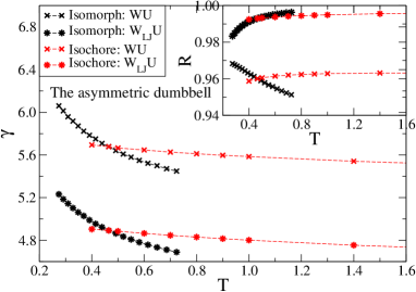
Figure 9: The variation of $\gamma$ [Eq. (16)] and the correlation coefficient $R$ [Eq. (1)] for the asymmetric dumbbell model in two different versions along an isochore (red, $\rho$ = 0.932) and along the isomorph (black) of Figs. 4-8. The crosses show $\gamma$ calculated from the total virial $W$ while the asterisks show $\gamma$ calculated after subtracting the constraint contribution to virial, i.e., $W_{LJ}=W-W_{CON}$. The corresponding $R$’s are shown in the insets. $\gamma$ is predicted in Ref. ¹⁵ to be a function only of density which is seen to apply to a good approximation for both versions.

Starting from an equilibrated sample at some state point, changing either temperature or density alters the equilibrium Boltzmann distribution of states. Two isomorphic state points have identical Boltzmann canonical probabilities (Eq. (8)). A sudden change of state from one state point to another isomorphic state point should thus not lead to any relaxation. This is called an isomorphic jump, and the prediction of no relaxation was shown in Ref. ¹⁵ to work well for the KABLJ liquid.

A similar numerical experiment is carried out for the asymmetric dumbbell model in Fig. 10. Considering three equilibrated, isochoric state points ($1$), ($2)$, and ($3$), the density and temperature are instantaneously changed to a state point ($4$). State point ($4$) is isomorphic to state point ($2$). The isomorph prediction is that jumps from state points ($1$) and ($3$) show relaxation, but not jumps from state point ($2$). This is indeed the case (Fig. 10(a)). State point ($1$) ages from below since the aging scheme ($1$) $\to$ ($4$) can be described as first an instantaneous isomorphic jump to the correct density, but a lower temperature, and subsequently relaxation from this state point along the isochore of state point ($4$).

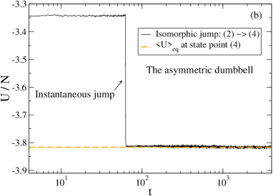
Figure 10: Four state points ($1$), ($2$), ($3$), and ($4$) corresponding to, respectively, ($\rho$, $T$) = ($0.932$, $0.400$), ($0.932$, $0.465$), ($0.932$, $2.000$), and ($0.851$, $0.274$) are given where the first three state points are on the same isochore. State points ($2$) and ($4$) are isomorphic, while ($1$) and ($3$) are not isomorphic to ($4$). After equilibrating at state points ($1$), ($2$), and ($3$), respectively, the temperature and density are instantaneously changed to that of state point ($4$) via a scaling of the coordinates keeping bond distances and Eulerian angles of the molecules fixed. An average has been performed over 100 samples. (a) The relaxational behaviour of all state points quantified by the potential energy $U$. The jump ($2$) $\to$ ($4$) shows no relaxation while the other state points do. (b) Close up of the potential energy of state point ($2$) before and after the jump, where the jump takes place at $t\approx 60$.

We finally consider the excess heat capacity per particle $C_{V}^{ex}/N$ in Fig. 11 along the isomorph and isotherm of Figs. 4-8. The excess heat capacity increases less than 2% along the isomorph, while the $12\%$ density increase on the isotherm results in a 25% increase in the excess heat capacity. This is consistent with the prediction in Sec. II that $C_{V}^{ex}/N$ is an isomorph invariant.

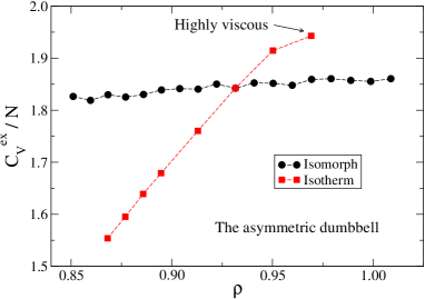
Figure 11: The excess heat capacity per particle $C_{V}^{ex}/N$ for the asymmetric dumbbell model as a function of density along the isomorph (black) and isotherm (red, $T$ = $0.465$) of Figs. 4-8. The density increase is 19% and 12%, respectively. The excess heat capacity increases less than 2% along the isomorph, while the isotherm shows a 25% increase. For the isotherm the dynamics becomes very slow for densities higher than $\rho=0.950$ and the system becomes difficult to equilibrate properly.

The previous figures show that isomorphs exists to a good approximation for the asymmetric dumbbell model. An important question is whether the specific molecular geometry determines whether or not a particular LJ model has good isomorphs. In Fig. 12 the correlation coefficient $R$ is given as a function of the bond length. The correlation coefficient decreases to $R\approx 0.65$ at unity bond length, and thus one might be tempted to conclude that LJ models with large bonds lengths in general do not have good isomorphs. In Sec. IV.3 we investigate the Lewis-Wahnström OTP model which have unity bond lengths and show that this model actually has good isomorphs. A theory connecting the variation of $R$ to the molecular geometry and/or bond lengths remains to be developed.

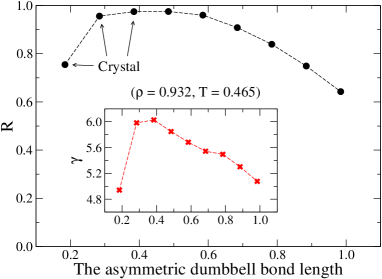
Figure 12: The correlation coefficient $R$ as a function of the bond length in the asymmetric dumbbell model at ($\rho$, $T$) = (0.932, 0.465). The investigated model has bond length $0.584$ with a correlation coefficient $R\approx 0.97$; however, as the bond length increases, the correlation coefficient decreases to $R\approx 0.65$ at unity bond length. The insets shows the corresponding values of $\gamma$ as defined in Eq. (16). As the bond length increase the system becomes very viscous and the statistics is poor at high bond lengths.

IV.2 Isomorphs of a symmetric IPL dumbbell model

In this section we briefly consider the isomorphs of a symmetric inverse power-law (IPL) dumbbell with exponent $n=18$ and bond length $0.584$. In Figs. 14(a) and (b) we show the particle radial distribution functions along an isomorph before and after scaling the distance $r$ into reduced units. Also shown is the reduced particle incoherent intermediate scattering function in Fig. 14(c).

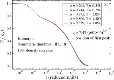
Figure 13: Structure and dynamics along an isomorph with 19% density increase for the symmetric IPL dumbbell model ($n=18$). (a) Particle pair-correlation function before scaling the distance $r$ into reduced units. (b) Particle pair-correlation function after scaling the distance $r$ into reduced units. (c) The reduced particle incoherent intermediate scattering function at constant reduced wavevector $q$.

The corresponding molecular center-of-mass quantities are shown in Fig. 14. Interestingly, the atomic dynamics appears more invariant than for the reduced molecular dynamics. The latter is predicted to be invariant along an isomorph while the former is not; however, we have not tried to quantify this observation any further.

Atomic systems with IPL interactions have exact isomorphs. This reflects the scale invariance of the IPL potential, i.e., that it preserves its shape under a scaling of the argument. Since molecules by their fixed geometry define a length scale in the system, isomorphs will always be approximate. However, the previous figures show that rigid molecules with IPL intermolecular interactions can also have good isomorphs.

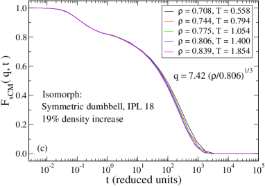
Figure 14: Structure and dynamics along the isomorph of Fig. 13 for the symmetric IPL dumbbell model ($n=18$). (a) Molecular center-of-mass pair-correlation function before scaling the distance $r$ into reduced units $\tilde{r}=\rho^{1/3}r$. (b) Molecular center-of-mass pair-correlation function after scaling the distance $r$ into reduced units. (c) The reduced molecular center-of-mass incoherent intermediate scattering function at constant reduced wavevector $q$.

In Fig. 15 we consider the variation of $\gamma$ and $R$ along the isomorph, which shows that $R$ decreases slightly with increasing temperature and density. The variation of $\gamma$ along the isomorph is less than for the asymmetric dumbbell, and is to a good approximation constant. As for the asymmetric dumbbell model (Fig. 9) the effect of the constraints is to increase $\gamma$ and decrease $R$ (these are respectively 6 and 1 for the IPL potential used).

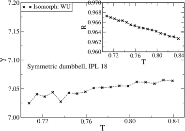
Figure 15: The variation of $\gamma$ and $R$ (insets) along the isomorph of Figs. 13-14 with 19% density increase for a symmetric dumbbell model ($n$ = $18$). $\gamma$ increases slightly along the isomorph. Excluding the constraints in the virial the correlation coefficient and $\gamma$ are respectively $R$ = $1$ and $\gamma$ = $6$.

IV.3 Isomorphs of the Lewis$-$Wahnström OTP model

We proceed to investigate the Lewis$-$Wahnström OTP model^{23; 24}. Figure 16 shows the particle radial distribution functions along an isomorph with 21% density increase before and after scaling the distance $r$ into reduced units. We treat the particles as identical in the quantities probed in simulations (i.e., the radial distribution function, etc.) even though the OTP model is an isosceles triangle. Also shown for reference is an isotherm with 11% density increase in Fig. 16(c).

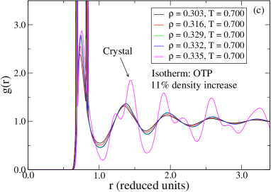
Figure 16: Particle radial distribution functions for the OTP model. (a) Along an isomorph with 21% density increase, shown prior to scaling the distance $r$ into reduced unit $\tilde{r}=\rho^{1/3}r$. (b) Along the same isomorph after scaling the distance $r$ into reduced unit. (c) Along an isotherm with 11% density increase. At the highest density probed the OTP model crystallizes³² (magenta).

Figure 17 shows the corresponding reduced molecular center-of-mass radial distribution functions. The reduced molecular center-of-mass structure seems less invariant along the isomorph than for the asymmetric dumbbell (Fig. 6), consistent with the OTP model being less strongly correlating ($R\approx 0.90$). However, comparing with the isotherm in Fig. 17(c) the OTP model crystallizes at the highest density probed³², even though the density increase is just 11% compared with the 21% density increase along the isomorph. Comparing now with the particle quantities of Fig. 16 the latter seems more invariant, even though the reduced molecular center-of-mass structure is predicted to be invariant. We currently have no explanation for this observation.

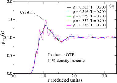
Figure 17: Molecular center-of-mass radial distribution functions for the OTP model. (a) Along the isomorph of Fig. 16 with 21% density increase, shown prior to scaling the distance $r$ into reduced units $\tilde{r}=\rho^{1/3}r$. (b) Along the same isomorph after scaling the distance $r$ into reduced units. (c) Along the isotherm of Fig. 16 with 11% density increase. At the highest density probed the OTP model here crystallizes (magenta).

Figure 18 shows the reduced particle incoherent intermediate scattering functions along the isotherm and isomorph of Figs. 16-17 while Fig. 19 shows the reduced molecular center-of-mass incoherent intermediate scattering functions.

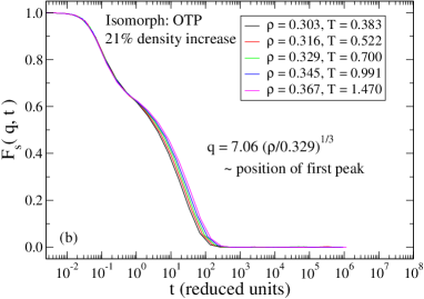
Figure 18: The reduced particle incoherent intermediate scattering functions for the OTP model keeping the reduced wavevector q constant. (a) Along the isotherm of Figs. 16-17 with 11% density increase. (b) Along the isomorph of Figs. 16-17 with 21% density increase and almost a factor of four increase in temperature. The dynamics is roughly invariant along the isomorph, but not along the isotherm.

For the molecular quantities, the dynamics is roughly invariant along the isomorph but not on the isotherm, even though the density increase is 21% for the isomorph and only 11% for the isotherm. In contrast to the reduced molecular center-of-mass structure; the molecular dynamics does not seem less invariant than the particle dynamics, consistent with the prediction of Appendix B.

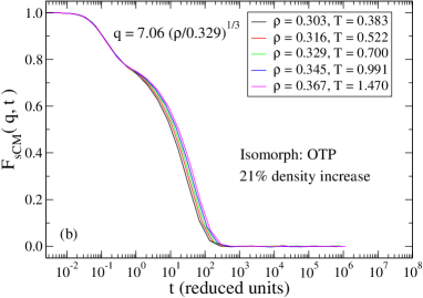
Figure 19: The reduced molecular center-of-mass incoherent intermediate scattering functions for the OTP model keeping the reduced wavevector q constant. (a) Along the isotherm of Figs. 16-18 with 11% density increase. (b) Along the isomorph of Figs. 16-18 with 21% density increase and almost a factor of four increase in temperature. The dynamics is roughly invariant along the isomorph, but not along the isotherm.

We consider in Fig. 20 the variation of $\gamma$ as defined by Eq. (16). The large variation in $\gamma$ indicates that density scaling, with a fixed exponent, is of more approximate nature for the OTP model²⁰ than for the asymmetric dumbbell, even though isomorphs exists to a good approximation. The isomorphs of the OTP model are, however, more approximative than for the asymmetric dumbbell, which is consistent with OTP model being less strongly correlating.

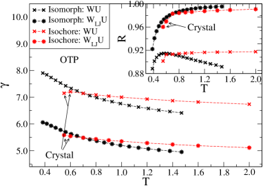
Figure 20: The variation of $\gamma$ (Eq. (16)) and the correlation coefficient $R$ (inset, Eq. (1)) for the OTP model in two different versions along an isochore (red, $\rho$ = $0.329$) and the isomorph (black) of Figs. 16-19. The crosses show $\gamma$ calculated from the total virial $W$, the asterisks show $\gamma$ calculated after subtracting the constraint contribution to virial, i.e., replacing $W$ by $W_{LJ}=W-W_{CON}$. $\gamma$ is predicted in Ref. ¹⁵ to be a function only of density as is seen to be the case for both versions, although the variation is larger than for the asymmetric dumbbell.

Next we consider isomorph jumps for the OTP model. The setup is analogous to that of the asymmetric dumbbell model described in Sec. IV.1. It is seen from Fig. 21 that an isomorph jump shows no relaxation.

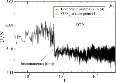
Figure 21: Four state points ($1$), ($2$), ($3$), and ($4$) corresponding to, respectively, ($\rho$, $T$) = ($0.329$, $0.650$), ($0.329$, $0.700$), ($0.329$, $1.000$), and ($0.303$, $0.383$) are given where the first three state points are on the same isochore. State points ($2$) and ($4$) are isomorphic while ($1$) and ($3$) are not isomorphic to ($4$). After equilibrating at state points ($1$), ($2$), and ($3$), respectively, the temperature and density are instantaneously changed to that of state point ($4$) via a scaling of the coordinates keeping bond distances and Eulerian angles of the molecules fixed. An average has been performed over 100 samples. (a) The relaxational behaviour of all state points quantified by the potential energy $U$. The jump ($2$) $\to$ ($4$) shows no relaxation while the other jumps do. (b) Close up of the potential energy of state point ($2$) before and after the jump, where the jump takes place at $t\approx 60$.

We close the investigation of the OTP model by considering in Fig. 22 the excess heat capacity per particle $C_{V}^{ex}/N$. This quantity increases 7% over the $21\%$ density increase along the isomorph, while the $11\%$ density increase on the isotherm results in a 34% increase before crystallizing. These results are consistent with the prediction that $C_{V}^{ex}$ is an isomorph invariant (see Sec. II), although less so than for the asymmetric dumbbell model.

Figure 22: The excess heat capacity per particle $C_{V}^{ex}/N$ for the OTP model as a function of density along the isomorph (black) and isotherm (red) of Figs. 16-19. The density increase is 21% and 11%, respectively. At high densities for the isotherm the OTP model crystallizes. The excess heat capacity is to a good approximation invariant along the isomorph, while this is not the case for the isotherm.

V Master isomorphs

The previous section detailed the existence of isomorphs in the phase diagram of liquids of small rigid molecules. We now investigate whether the generated isomorphs have the same shape in the $WU$ phase diagram, i.e., whether a so-called master isomorph exists¹⁶. It is also interesting to compare the isomorphs of the dumbbell and the OTP models, since both systems have intermolecular ($12$, $6$)-LJ interactions, but different constraint contributions to the virial (one versus three constrained distances per molecule).

Figure 23(a) shows three different isomorphs in the $WU$ phase diagram for the asymmetric dumbbell model, in two different versions: one for the total virial $W$ and one for the ”LJ” virial, i.e., replacing $W$ with $W_{LJ}=W-W_{CON}$. In order to investigate whether a master isomorph exists Fig. 23(b) shows the same isomorphs after scaling of the potential energy and the virial with the same factor (depending on the isomorph). The best scaling factor was identified by trial and error.

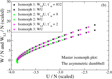
Figure 23: (a) Three different isomorphs for the asymmetric dumbbell model in two different versions with 19%, 21% and 22% density increase, respectively (black, magenta and green). The crosses give the total virial $W$, the asterisks give $W_{LJ}=W-W_{CON}$. $\tilde{\tau}_{\alpha}$ is reduced relaxation time extracted from the self part of the intermediate scattering function. (b) The same isomorphs as in (a) where $WU$ and $W_{LJ}U$ are scaled to superpose with a factor identified by trial and error. The black points have unity scaling factor.

Corresponding figures for the OTP system are given in Fig. 24. The figures show that for both models a master isomorph exists to a good approximation both with and without the constraint contribution to the virial.

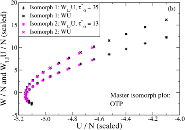
Figure 24: (a) Two different isomorphs for the OTP model in two different versions with 21% and 14% density increase (black and magenta). The crosses give the total virial $W$, the asterisks give $W_{LJ}=W-W_{CON}$. $\tilde{\tau}_{\alpha}$ is reduced relaxation time extracted from the self part of the intermediate scattering function. (b) The same isomorphs as in (a) where $WU$ and $W_{LJ}U$ are scaled to superpose with a factor identified by trial and error. The black points have unity scaling factor.

As mentioned in the introduction, Ref. ¹⁶ derived predictions concerning the shape of isomorphs for atomic systems with pair potential given by a sum of two IPLs (the generalized LJ potential). The question arises whether $W_{LJ}U$ follows that shape? This is studied in Fig. 25(a) where the $W_{LJ}U$ isomorphs for the asymmetric dumbbell and OTP models are shown scaled using the previously mentioned procedure. The two dashed curves are the isomorph prediction for an atomic ($12$, $6$)-LJ system ¹⁶ (where $\tilde{\rho}=\rho/\rho^{*}$ and $\rho^{*}$ is the density of a chosen reference state point)

$$U =U_{m}^{*}\tilde{\rho}^{4}+U_{n}^{*}\tilde{\rho}^{2},$$ (18)

$$W_{LJ} =4U_{m}^{*}\tilde{\rho}^{4}+2U_{n}^{*}\tilde{\rho}^{2},$$ (19)

where the reference coefficients ($U_{m}^{*}$, $U_{n}^{*}$) have been calculated from two different reference state points along ”Isomorph 1” of the asymmetric dumbbell (see Ref. ¹⁶ for details on calculating these coefficients). The only assumption used in Ref. ¹⁶ to derive these formulas is the invariance of the reduced atomic structure along an isomorph, however, this is not predicted to be the case for molecular systems with isomorphs.

It is clear that the atomic isomorph shape is not followed exactly. Nevertheless, there seems to exist not only a master isomorph in the LJ and total virial for the individual systems, but also for the LJ virial between these two different model systems. The same does not hold for the total virial as can been seen in Fig. 25(b) since the constraint contributions are different.

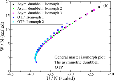
Figure 25: (a) Scaled $W_{LJ}U$ isomorphs for the asymmetric dumbbell and OTP models. The black points have unity scaling factor. Both systems have intermolecular ($12$, $6$)-LJ interactions, and the dashed curves are the isomorph prediction from Ref. ¹⁶ for an atomic system, where the LJ reference coefficients have respectively been calculated from the dumbbell state points ($\rho$, $T$) = ($0.932$, $0.465$) and ($0.851$, $0.274$). (b) Scaled $WU$ isomorphs for the systems in (a). The total virial does not show exact scaling between the asymmetric dumbbell and OTP models.

To examine the extent of ”deviation” from Eqs. (18) and (19) we show in Fig. 26 for the asymmetric dumbbell $U$ and $W_{LJ}$ as a function of the reduced density $\tilde{\rho}^{2}$ ($\rho^{*}=1$). The reference coefficients can be calculated from a linear regression fit of the potential energy and the estimated coefficients can be used to plot a straight line in the LJ virial plot. This is performed in Fig. 26 where it is clear that even though both plots follow a near straight-line, the coefficients are not given by Eqs. (18) and (19). It is worth mentioning again that the prediction of Ref. ¹⁶ is for an atomic system, and is as such not excepted to hold for rigid molecular systems.

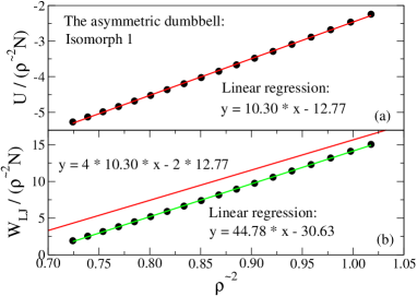
Figure 26: The potential energy and LJ virial as a function of $\tilde{\rho}^{2}$ for ”Isomorph 1” of the asymmetric dumbbell. (a) A linear regression fit of the potential energy has been performed to calculate the reference coefficients ($U_{m}^{*}$, $U_{n}^{*}$). (b) These coefficients are then used to plot the red straight line, which according to the atomic prediction [Eqs. (18) and (19)] should coincide with the black data points. The green line is a linear regression fit to the same data points.

Finally we consider in Fig. 27 for the asymmetric dumbbell how the instantaneous fluctuations of $W_{CON}$ correlate with $W_{LJ}$ and $W$ respectively. The constraint contribution to the virial at this state point does not correlate well with the contribution to the virial coming from the LJ interactions ($R$ = $0.31$). Obviously, the correlation is higher when the total virial is considered ($R$ = $0.61$). The main contribution to the virial, for the asymmetric dumbbell model, comes from the LJ interactions, however, the LJ virial does not correlate well with the constraint virial. The latter observation may indicate a break-down of master isomorph scaling (for the total virial) at high pressures, however, this remains to be confirmed.

Figure 27: (a) The correlation of the instantaneous fluctuations of $W_{LJ}$ and $W_{CON}$. The correlation coefficient $R$ is 0.31. (b) The correlation of the instantaneous fluctuations of $W$ and $W_{CON}$. The correlation coefficient $R$ is 0.61.

VI Summary and outlook

Isomorphs are curves in the phase diagram of a strongly correlating liquid along which a number of static and dynamic quantities are invariant in reduced units. References ¹⁵ and ¹⁶ focused on understanding isomorphs in atomic systems. In this paper we generalized the isomorph concept to deal with systems of rigid molecules [Eq. (5)] and investigated several isomorph invariants for the asymmetric dumbbell model and the Lewis-Wahnström OTP model. We find that these rigid molecular systems also have isomorphs to a good approximation; however, the isomorphs of the OTP model were more approximative than those of the asymmetric dumbbell, consistent with the OTP model being less strongly correlating. Moreover, it was found that these systems to a good approximation have master isomorphs, i.e., that all isomorphs have the same shape in the virial/potential energy phase diagram. This applies for the total virial, but also after subtracting the constraint contribution. A general master isomorph was identified between the investigated model systems after this subtraction. We do not at the present have an explanation for this observation.

A full theoretical understanding of the implications of rigid bonds remains to be arrived at. For instance, the shape of molecular isomorphs is different from the shape of Ref. ¹⁶ for atomic isomorphs. The rigid bonds seem in general to increase $\gamma$ and decrease the correlation coefficient $R$ with respect to the unconstrained system. More specific; $R$ decreases significantly with increasing asymmetric dumbbell bond length ($R\approx 0.65$ around unity bond length, see Sec. IV.1). This is consistent with the results of Chopra et al.¹⁰, who note a worse scaling of the reduced relaxation time and diffusion constant with (excess) entropy based quantities when increasing the bond length of a rigid symmetric LJ dumbbell model. On the other hand, it is noteworthy that strong correlation is observed for the OTP model even though it has unity bond lengths. The molecular center-of-mass structure in reduced units is predicted to be invariant along an isomorph, however, for the OTP model the reduced particle structure seems more invariant along an isomorph than the reduced molecular center-of-mass structure. The former is not predicted to be invariant along an isomorph, and thus the observed difference should be investigated in more detail to clarify this issue.

Appendix A Constrained dynamics and the virial

Constrained dynamics is discussed in many different places, see for instance Refs. ³⁴, ⁴¹, and ⁴². We give here a brief introduction to constrained dynamics and the connection to the virial expression used in this article.

Gauss’ principle of least constraint⁴⁴ states that a classical mechanical system of $N$ particles with constraints deviates instantaneously in a least possible sense from Newton’s 2nd law, i.e., that

$$\sum_{i=1}^{N}m_{i}\Big{[}\ddot{\textbf{r}}_{i}-\frac{\textbf{F}_{i}}{m_{i}}\Big{]}^{2},$$ (20)

is a minimum. Here $\textbf{r}_{i}$ and $\textbf{F}_{i}$ are the position and interaction force of particle $i$. In the case of no constraints, setting the partial derivative $\partial/\partial\ddot{\textbf{r}}_{i}$ to zero implies $\ddot{\textbf{r}}_{i}-\textbf{F}_{i}/m_{i}=0$, i.e., Newtons’s 2nd law.

In the case of holonomic constraints $\psi^{\alpha}(\textbf{r}^{N})=0$ where $\alpha=1,...,G$, the variation can be carried out by introducing Lagrangian multipliers, i.e.,

$$\sum_{i=1}^{N}m_{i}\Big{[}\ddot{\textbf{r}}_{i}-\frac{\textbf{F}_{i}}{m_{i}}\Big{]}^{2}-\sum_{\alpha=1}^{G}\lambda^{\alpha}\ddot{\psi}^{\alpha},$$ (21)

should be a minimum. Setting the partial derivative $\partial/\partial\ddot{\textbf{r}}_{i}$ to zero implies (where the factor of one half has been absorbed in the Lagrangian multiplier)

$$m_{i}\cdot\ddot{\textbf{r}}_{i}=\textbf{F}_{i}+\sum_{\alpha=1}^{G}\lambda^{\alpha}\nabla_{\textbf{r}_{i}}\psi^{\alpha}=\textbf{F}_{i}+\textbf{G}_{i}.$$ (22)

Newton’s 2nd law thus remains valid if an additional force is added (called the constraint force $\textbf{G}_{i}$). At this point $\lambda^{\alpha}$ is undetermined; however, an explicit expression⁴¹ for $\lambda^{\alpha}$ can be determined from the condition $\textbf{r}_{ij}\cdot\ddot{\textbf{r}}_{ij}+\dot{\textbf{r}}_{ij}^{2}=0$. In molecular dynamics simulations it is imperative to calculate $\lambda^{\alpha}$ correctly to achieve a stable numerical algorithm. The reader is referred to Refs. ³⁴ and ³⁵ for details concerning this aspect.

The virial $W$ is defined by $W$ = $1/3\sum_{i=1}^{N}\textbf{r}_{i}\cdot\textbf{F}_{i}$. In an atomic system with LJ pair potential interactions the virial is given by $W=W_{LJ}=-1/3\sum_{i<j}^{N}r_{ij}u^{\prime}(r_{ij})$. If the system has bond constraints $\psi^{\alpha}$ = $(\textbf{r}_{\alpha,i}-\textbf{r}_{\alpha,j})^{2}/2$ = $\textbf{r}^{2}_{\alpha,ij}$/2 = $c_{\alpha,ij}^{2}/2$ it follows from Eq. (22) that the constraint force contributes to the virial as $W_{CON}=1/3\sum_{i=1}^{N}\textbf{r}_{i}\cdot\textbf{G}_{i}=1/3\sum_{\alpha=1}^{G}\lambda^{\alpha}\textbf{r}_{\alpha,ij}^{2}$.

Appendix B Constrained NVE and Nos$\acute{e}$-Hoover NVT dynamics in reduced units along an isomorph

We start our considerations of this section from the constrained equations of motion derived in Appendix A, Eq. (22):

$$m_{i}\cdot\ddot{\textbf{r}}_{i}=\textbf{F}_{i}+\sum_{\alpha=1}^{G}\lambda^{\alpha}\nabla_{\textbf{r}_{i}}\psi^{\alpha}=\textbf{F}_{i}+\textbf{G}_{i}.$$ (23)

Here $\textbf{r}_{i}$ and $\textbf{F}_{i}$ are, respectively, the position and interaction force of particle $i$, and $\lambda^{\alpha}$ a Lagrangian multiplier for the $\alpha$’te constraint $\psi^{\alpha}$. For simulating rigid molecules⁴⁵ the constraints would in general be a combination of constrained bond lengths $\psi^{\alpha}$ = $(\textbf{r}_{\alpha,i}-\textbf{r}_{\alpha,j})^{2}/2$ = $\textbf{r}^{2}_{\alpha,ij}$/2 = $c_{\alpha,ij}^{2}/2$ and linear constraints $\psi^{\beta}=\sum_{i=1}^{n_{b}}C_{\beta i}\textbf{r}_{i}-\textbf{r}_{\beta}=0$, where $C_{\beta i}$ is a factor that depends on the geometry of the molecule (see Ref. ⁴⁵ for more details). For simplicity we consider only bond constraints in the following.

A general expression for the Lagrange multiplier $\lambda^{\alpha}$ can be derived and is given by^{41; 46}

$$\lambda^{\alpha} =-\sum_{\beta=1}^{G}\big{(}\textbf{Z}^{-1}\big{)}_{\alpha\beta}\Big{[}\sum_{i,j=1}^{N}\nabla_{\textbf{r}_{i}}\nabla_{\textbf{r}_{j}}\psi^{\beta}\dot{\textbf{r}}_{j}\dot{\textbf{r}}_{i}+\sum_{i=1}^{N}\frac{\nabla_{\textbf{r}_{i}}\psi^{\beta}\cdot\textbf{F}_{i}}{m_{i}}\Big{]},$$ (24)

$$Z_{\alpha\beta} =\sum_{i=1}^{N}\frac{\nabla_{\textbf{r}_{i}}\psi^{\alpha}\cdot\nabla_{\textbf{r}_{i}}\psi^{\beta}}{m_{i}}.$$ (25)

Defining reduced units for length, energy, and mass as follows

$$\tilde{\textbf{r}}_{i} =\rho^{1/3}\textbf{r}_{i},$$ (26)

$$\tilde{U} =U/k_{B}T,$$ (27)

$$\tilde{m}_{i} =m_{i}/\langle m\rangle,$$ (28)

reduced units for time and force follow as

$$\tilde{t} =t/\big{(}\rho^{-1/3}\sqrt{\langle m\rangle/k_{B}T}\big{)},$$ (29)

$$\tilde{\textbf{F}}_{i} =\rho^{-1/3}\textbf{F}_{i}/k_{B}T=-\nabla_{\tilde{\textbf{r}}_{i}}U/k_{B}T.$$ (30)

Inserting the above definitions in Eqs. (23) - (25) and using that $\nabla_{\textbf{r}_{i}}\psi^{\alpha}=\textbf{r}_{\alpha,ij}$, we arrive at the constrained NVE equations of motion in reduced units

$$\tilde{m}_{i}\cdot\ddot{\tilde{\textbf{r}}}_{i}=\tilde{\textbf{F}}_{i}+\sum_{\alpha=1}^{G}\tilde{\lambda}^{\alpha}\tilde{\textbf{r}}_{\alpha,ij}=\tilde{\textbf{F}}_{i}+\tilde{\textbf{G}}_{i},$$ (31)

where

$$\tilde{\lambda}^{\alpha} =-\sum_{\beta=1}^{G}\big{(}\tilde{\textbf{Z}}^{-1}\big{)}_{\alpha\beta}\Big{[}\sum_{i,j=1}^{N}\dot{\tilde{\textbf{r}}}_{j}\dot{\tilde{\textbf{r}}}_{i}+\sum_{i=1}^{N}\frac{\tilde{\textbf{r}}_{\beta,ij}\cdot\tilde{\textbf{F}}_{i}}{\tilde{m}_{i}}\Big{]},$$ (32)

$$\tilde{Z}_{\alpha\beta} =\sum_{i=1}^{N}\frac{\tilde{\textbf{r}}_{\alpha,ij}\tilde{\textbf{r}}_{\beta,ij}}{\tilde{m}_{i}}.$$ (33)

Since in general $\tilde{\textbf{r}}_{\alpha,ij}^{2}=\rho^{2/3}c_{\alpha,ij}^{2}$ the reduced constrained equations of motion are not invariant along an isomorph.

Considering instead the molecular center-of-mass motion in reduced units

$$\tilde{M}_{i}\cdot\ddot{\tilde{\textbf{r}}}_{CM,i}=\tilde{\textbf{F}}_{CM,i},$$ (34)

where $\tilde{\textbf{F}}_{CM,i}$ and $\tilde{M}_{i}$ are, respectively, the reduced force and mass of molecule $i$. Since the reduced force $\tilde{\textbf{F}}_{CM,i}$ is invariant along an isomorph, it follows that the molecular NVE equations of motion are invariant along an isomorph. The invariance of $\tilde{\textbf{F}}_{CM,i}$ can be seen as follows. The isomorph definition Eq. (5) implies for a fixed state point ($1$) and arbitrary state point ($x$), both along the same isomorph [where $\tilde{\textbf{R}}$ $\equiv$ ($\rho^{-1/3}\tilde{\textbf{r}}_{CM,1}$, $\theta_{1}$, $\phi_{1}$, $\psi_{1}$, …, $\rho^{-1/3}\tilde{\textbf{r}}_{CM,N}$, $\theta_{N}$, $\phi_{N}$, $\psi_{N}$)]

$$-U(\tilde{\textbf{R}}^{(x)})/k_{B}T_{x}=-U(\tilde{\textbf{R}}^{(1)})/k_{B}T_{1}-\ln\,C_{1x}.$$ (35)

Taking the gradient $\nabla_{\tilde{\textbf{r}}_{CM,i}}$ it follows that

$$\tilde{\textbf{F}}_{CM,i}^{(x)}=\tilde{\textbf{F}}_{CM,i}^{(1)}.$$ (36)

This concludes the proof of the isomorph invariance of the reduced molecular center-of-mass equations of motion. A similar situation is given for the constrained NVT equations of motion, however; considering the molecular motion, the constraint force disappears, and the proof in analogous to the above and shown for atomic systems in Ref. ¹⁵. In this case the time-constant of the Nos$\acute{e}$-Hoover algorithm needs to be adjusted along the isomorph, otherwise the dynamics is not invariant.

References

- Alba-Simionesco et al. (2004) Alba-Simionesco, C.; Cailliaux, A.; Alegría, A.; Tarjus, G. Europhys. Lett. 2004, 68, 58.
- Dreyfus et al. (2004) Dreyfus, C.; Grand, A. L.; Gapinski, J.; Steffen, W.; Patkowski, A. Eur. Phys. J. B 2004, 42, 309.
- Roland (2010) Roland, C. M. Macromolecules 2010, 43, 7875.
- Roland et al. (2003) Roland, C. M.; Casalini, R.; Paluch, M. Chem. Phys. Lett. 2003, 367, 259.
- Ngai et al. (2005) Ngai, K. L.; Casalini, R.; Capaccioli, S.; Paluch, M.; Roland, C. M. J. Phys. Chem. B 2005, 109, 17356.
- Rosenfeld (1977) Rosenfeld, Y. Phys. Rev. A 1977, 15, 2545.
- Rosenfeld (1999) Rosenfeld, Y. J. Phys.: Condens. Matter 1999, 11, 5415.
- Chopra et al. (2010) Chopra, R.; Truskett, T. M.; Errington, J. R. J. Phys. Chem. B 2010, 114, 10558.
- Chopra et al. (2010) Chopra, R.; Truskett, T. M.; Errington, J. R. J. Phys. Chem. B 2010, 114, 16487.
- Chopra et al. (2010) Chopra, R.; Truskett, T. M.; Errington, J. R. J. Chem. Phys. 2010, 133, 104506.
- Galliero et al. (2011) Galliero, G.; Boned, C.; Fernndez, J. J. Phys. Chem. 2011, 134, 064505.
- Bailey et al. (2008) Bailey, N. P.; Pedersen, U. R.; Gnan, N.; Schrøder, T. B.; Dyre, J. C. J. Chem. Phys. 2008, 128, 184507.
- Bailey et al. (2008) Bailey, N. P.; Pedersen, U. R.; Gnan, N.; Schrøder, T. B.; Dyre, J. C. J. Chem. Phys. 2008, 129, 184508.
- Schrøder et al. (2009) Schrøder, T. B.; Bailey, N. P.; Pedersen, U. R.; Gnan, N.; Dyre, J. C. J. Chem. Phys. 2009, 131, 234503.
- Gnan et al. (2009) Gnan, N.; Schrøder, T. . B.; Pedersen, U. R.; Bailey, N. P.; Dyre, J. C. J. Chem. Phys. 2009, 131, 234504.
- Schrøder et al. (2011) Schrøder, T. B.; Gnan, N.; Pedersen, U. R.; Bailey, N. P.; Dyre, J. C. J. Chem. Phys. 2011, 134, 164505.
- Pedersen et al. (2008) Pedersen, U. R.; Bailey, N. P.; Schrøder, T. B.; Dyre, J. C. Phys. Rev. Lett. 2008, 100, 015701.
- Coslovich and Roland (2009) Coslovich, D.; Roland, C. M. J. Chem. Phys. 2009, 130, 014508.
- Coslovich and Roland (2008) Coslovich, D.; Roland, C. M. J. Phys. Chem. B 2008, 112, 1329.
- Schrøder et al. (2009) Schrøder, T. B.; Pedersen, U. R.; Bailey, N. P.; Toxvaerd, S.; Dyre, J. C. Phys. Rev. E 2009, 80, 041502.
- Kob and Andersen (1995) Kob, W.; Andersen, H. C. Phys. Rev. E 1995, 51, 4626.
- Kob and Andersen (1995) Kob, W.; Andersen, H. C. Phys. Rev. E 1995, 52, 4134.
- Wahnström and Lewis (1993) Wahnström, G.; Lewis, L. J. Physica A 1993, 201, 150.
- Lewis and Wahnström (1994) Lewis, L. J.; Wahnström, G. Phys. Rev. E 1994, 50, 3865.
- Gundermann et al. (2011) Gundermann, D.; Pedersen, U. R.; Hecksher, T.; Bailey, N. P.; Jakobsen, B.; Christensen, T.; Olsen, N. B.; Schrøder, T. B.; Fragiadakis, D.; Casalini, R.; Roland, C. M.; Dyre, J. C.; Niss, K. Nature Physics 2011, DOI: 10.1038.
- Pedersen et al. (2011) Pedersen, U. R.; Schrøder, T. B.; Bailey, N. P.; Toxvaerd, S.; Dyre, J. C. J. of Non-Crystalline Solids 2011, 357, 320.
- (27) In practice it’s only required that the physically relevant configurations obey this scaling, i.e., at least those that contribute significantly to the partition function.
- Goldstein et al. (2002) Goldstein, H.; Poole, C.; Safko, J. Classical Mechanics, 3rd ed.; Addison Wesley, 2002.
- Gray and Gubbins (1984) Gray, C. G.; Gubbins, K. E. Theory of Molecular Fluids; Oxford University Press, 1984.
- Lazaridis and Paulaitis (1992) Lazaridis, T.; Paulaitis, M. E. J. Phys. Chem. 1992, 96, 3847.
- Lazaridis and Karplus (1996) Lazaridis, T.; Karplus, M. J. Chem. Phys. 1996, 105, 4294.
- Pedersen et al. (2011) Pedersen, U. R.; Hudson, T. S.; Harrowell, P. J. Chem. Phys. 2011, 134, 114501.
- Hess et al. (2008) Hess, B.; Kutzner, C.; van der Spoel, D.; Lindahl, E. J. Chem. Theory Comput. 2008, 4, 435.
- Toxvaerd et al. (2009) Toxvaerd, S.; Heilmann, O. J.; Ingebrigtsen, T.; Schrøder, T. B.; Dyre, J. C. J. Chem. Phys. 2009, 131, 064102.
- Ingebrigtsen et al. (2010) Ingebrigtsen, T.; Heilmann, O. J.; Toxvaerd, S.; Dyre, J. C. J. Chem. Phys 2010, 132, 154106.
- Nos (1984) Nos, S. J. Chem. Phys. 1984, 81, 511.
- Hoover (1985) Hoover, W. G. Phys. Rev. A 1985, 31, 1695.
- Toxvaerd (1991) Toxvaerd, S. Mol. Phys. 1991, 72, 159.
- (39) All simulations were performed using a molecular dynamics code optimized for NVIDIA graphics cards, which is available as open source code at www.rumd.org.
- Frenkel and Smit (2002) Frenkel, D.; Smit, B. Understanding Molecular Simulation; Academic Press, 2002.
- Edberg et al. (1986) Edberg, R.; Evans, D. J.; Morriss, G. P. J. Chem. Phys. 1986, 84, 6933.
- Ryckaert et al. (1977) Ryckaert, J. P.; Ciccotti, G.; Berendsen, H. J. C. J. Comput. Phys. 1977, 23, 327.
- Fragiadakis and Roland (2011) Fragiadakis, D.; Roland, C. M. J. Chem. Phys. 2011, 134, 044504.
- Gauss (1829) Gauss, K. F. J. Reine Angew. Math. 1829, 4, 232.
- Ciccotti et al. (1982) Ciccotti, G.; Ferrario, M.; Ryckaert, J. P. Mol. Phys. 1982, 47, 1253.
- Melchionna (2000) Melchionna, S. Phys. Rev. E 2000, 61, 6165.