The DiskMass Survey. IV. The Dark-Matter-Dominated Galaxy UGC 463

Abstract

We present a detailed and unique mass budget for the high-surface-brightness galaxy UGC 463, showing it is dominated by dark matter (DM) at radii beyond one scale length ($h_{R}$) and has a baryonic-to-DM mass ratio of approximately 1:3 within 4.2$h_{R}$. Assuming a constant scale height ($h_{z}$, calculated via an empirical oblateness relation), we calculate dynamical disk mass surface densities from stellar kinematics, which provide vertical velocity dispersions after correcting for the shape of the stellar velocity ellipsoid (measured to have $\sigma_{\theta}/\sigma_{R}=1.04\pm 0.22$ and $\sigma_{z}/\sigma_{R}=0.48\pm 0.09$). We isolate the stellar mass surface density by accounting for all gas mass components and find an average $K$-band mass-to-light ratio of $0.22\pm 0.09(ran)~{}^{+0.16}_{-0.15}(sys)~{}\mathcal{M}_{\odot}/\mathcal{L}_{\odot}^{K}$; Zibetti et al. and Bell et al. predict, respectively, 0.56 and 3.6 times our dynamical value based on stellar-population-synthesis modeling. The baryonic matter is submaximal by a factor of $\sim 3$ in mass and the baryonic-to-total circular-speed ratio is $0.61^{+0.07}_{-0.09}(ran)~{}^{+0.12}_{-0.18}(sys)$ at 2.2$h_{R}$; however, the disk is globally stable with a multi-component stability that decreases asymptotically with radius to $Q\sim 2$. We directly calculate the circular speed of the DM halo by subtracting the baryonic contribution to the total circular speed; the result is equally well described by either a Navarro-Frenk-White halo or a pseudo-isothermal sphere. The volume density is dominated by DM at heights of $|z|\gtrsim 1.6h_{z}$ for radii of $R\gtrsim h_{R}$. As is shown in follow-up papers, UGC 463 is just one example among nearly all galaxies we have observed that contradict the hypothesis that high-surface-brightness spiral galaxies have maximal disks.

1. Introduction

A primary goal of modern extragalactic astronomy is to reduce the complex, stochastic process of galaxy formation into a few fundamental physical parameters. Such a goal appears tractable given the tight scaling relations exhibited by galaxies over a large dynamic range in observed properties, which to first order may be tied to a single physical characteristic (Disney et al., 2008). For example, measures of galaxy size, luminosity, and a virialized dynamical quantity (such as the circular velocity in rotationally supported systems and velocity dispersion in pressure-dominated systems) demonstrate strong covariance. Correlations among galaxy properties are found in two-dimensional scatter plots (e.g., Courteau et al., 2007; Nair et al., 2010; Saintonge & Spekkens, 2011), lines through multi-dimensional space (e.g., Tollerud et al., 2011), and more complex, multi-dimensional manifolds (e.g., Zaritsky et al., 2008). Empirical and theoretical understanding of these relations over cosmic time (as in, e.g., Dutton et al., 2011a) are critical.

Two long-standing scaling relations are the Tully–Fisher relation (Tully & Fisher, 1977, hereafter the TF relation) — the correlation between the rotation velocity of spiral galaxies and their total luminosity — and the Fundamental Plane (FP; Dressler et al., 1987; Djorgovski & Davis, 1987) — the plane relating the size, surface brightness, and velocity dispersion of elliptical galaxies. These fundamental relations are strongly linked to mass: The baryonic TF (BTF) relation (McGaugh et al., 2000; McGaugh, 2005), created by replacing total luminosity with total baryonic mass, exhibits less scatter than the nominal TF relation over a wide range of luminosity and spiral type. The mass-based FP (Bolton et al., 2007), incorporating the total (baryonic$+$dark-matter[DM]) mass surface density instead of surface brightness, also exhibits lower scatter than its luminosity-based counterpart. It is interesting that the residuals are reduced for both the BTF and mass-based FP relation despite the exclusion of DM from the former. The tightness of the BTF implies that either DM is a rather negligible mass component or there exists a strict proportionality, in both relative amplitude and distribution, between DM and baryonic mass in spiral galaxies. The former is incompatible with our current understanding of gravity and the current paradigm of hierarchical disk-galaxy formation (see, e.g., Fall & Efstathiou, 1980; Dalcanton et al., 1997; Mo et al., 1998; Agertz et al., 2011), and the latter is tantamount to the discomforting disk-halo conspiracy (van Albada & Sancisi, 1986, hereafter vAS86). One can begin to address this contentious issue by placing direct constraints on the detail mass composition of galaxies.

Although there are multiple methods of measuring the total mass enclosed within a given radius (e.g., dynamics, lensing), a robust decomposition of total mass into fractional contributions from DM, stars, and the interstellar medium (ISM) is non-trivial. Measurements of the atomic-gas mass can be made directly using 21cm H i emission, and molecular-gas mass can be estimated using CO emission. However, stellar mass estimates depend on the calibration of stellar mass-to-light ratios, $\Upsilon_{\ast}$, via resolved stellar populations in the most nearby (dwarf) galaxies or stellar-population-synthesis (SPS) modeling of integrated light. The latter remains substantially uncertain (Conroy et al., 2009, 2010; Conroy & Gunn, 2010).

Rotation-curve mass decompositions provide upper limits on $\Upsilon_{\ast}$ when one adopts the “maximum-disk” hypothesis, the assumption that the rotation velocity at the center is dominated by the luminous matter (vAS86). For example, Bell & de Jong (2001) used the “maximum-disk” rotation curve decompositions made by Verheijen (2001, hereafter V01) to place limits on the allowed $\Upsilon_{\ast}$. However, rotation curves cannot provide unique measurements of $\Upsilon_{\ast}$ as we have recently illustrated (Bershady et al., 2010a, hereafter Paper I); inference of $\Upsilon_{\ast}$ based on rotation-curve mass decompositions are unconstrained due to the disk-halo degeneracy (van Albada et al., 1985).

Given the uncertainty in SPS model zero-points and the disk-halo degeneracy, a direct measurement of $\Upsilon_{\ast}$ is needed. Following the work of Bahcall & Casertano (1984), van der Kruit & Freeman (1984, 1986), and Bottema (1993), the DiskMass Survey (DMS; Paper I, ) aims to tackle this problem via dynamical measurements of the mass surface density, $\Sigma_{\rm dyn}$, of $\gtrsim$40 low-inclination, late-type galaxies. Our measurements uniquely describe the baryonic mass distributions and DM-halo density profiles, $\rho_{\rm DM}$, of each galaxy within $\sim$3 disk scale lengths ($h_{R}$), thereby breaking the disk-halo degeneracy and allowing for detailed calculations of disk-galaxy mass budgets. In this paper, we focus on providing a detailed, initial example of these calculations using UGC 463, located at equatorial (J2000.0) coordinates (RA,DEC) = (00^h43^m32$\fs$5,+14^d20^m34^s). We continue our series by summarizing the baryonic mass fractions in 29 additional galaxies in Bershady et al. (2011; hereafter Paper V), submitted.

Here we summarize some salient properties of UGC 463: It is a well isolated galaxy with a moderately-high extrapolated central disk surface brightness (Paper I), which is a factor of $\sim 2$ above the mean derived by Freeman (1970). It is of late type (SABc; Paper I, ) and demonstrates an interesting three-arm spiral structure. The SDSS $g$-band surface photometry demonstrates a clear Type II surface-brightness profile, as defined by Freeman (1970), with a profile “break” at a radius of $\sim 15\arcsec$, well within the field-of-view (FOV) of our kinematic data; the break becomes less pronounced toward longer wavelengths. The disk is also bright in the mid- and far-infrared Spitzer bands, suggestive of significant star-formation activity and molecular gas mass. In general, UGC 463 is unexceptional in its optical and near-infrared (NIR) color, size, and luminosity; however, it is slightly redder and more luminous (in $M_{K}$) than typical of galaxies in the DMS Phase-B sample (as defined in Paper I, ).

Our study of UGC 463 is a detailed example in the use of our full suite of data to produce quantities of fundamental relevance to the science goals of the DMS (Paper I), following much of the formalism developed in Bershady et al. (2010b, hereafter Paper II). Given the large number of observational ingredients, we have relocated some detailed information to future papers, which we refer to throughout our discussion. An outline of our paper is as follows: Section 2 presents all the data products. We derive the on-sky geometric projection of the disk using our two-dimensional kinematic data in Section 3, including an extensive discussion of the inclination, $i$. Based on this projection geometry, we produce azimuthally averaged kinematic profiles and beam-smearing corrections and discuss the axial symmetry of the galaxy in Section 4. In Section 5, we derive salient properties of the disk including the shape of the disk stellar velocity ellipsoid (SVE), the disk stability, mass surface densities of all baryonic components, and dynamical mass-to-light ratios. In Section 6, we produce a detailed mass budget for UGC 463 out to 15 kpc ($\sim 4.2$ scale lengths); this analysis relies on a traditional rotation-curve mass decomposition but uses our direct measurements of $\Upsilon_{\ast}$. Having established the mass distribution of all the baryonic components, Section 6 also presents the DM-halo density and enclosed-mass distribution. Therefore, Sections 2 – 4 are largely concerned with data handling, whereas Sections 5 – 6 produce the scientifically motivated calculations that result from these data. We summarize our study in Section 7.

We note here the nomenclature $\epsilon(x)$ signifies the measurement error in $x$, $\overline{x}$ is the azimuthal average of $x$, and $\langle x\rangle$ is the combined radial and azimuthal average of $x$. When quoting two sets of errors in any quantity (as done in the Abstract), the first and second set provide the random and systematic uncertainties, respectively.

2. Observational Data

The DMS has collected an extensive suite of data to reach our science goals, as described in Paper I. We draw upon a large fraction of those observations specific to UGC 463 for use in this paper. Table 1 provides a list of all the data products used herein, their observational source, the year of the relevant observations, a reference to the section containing a description of each dataset, and (when available) a reference to papers containing more detailed information. On-sky maps of much of the relevant data products are provided in Figure 1; see Section 3.3 and Appendix A for a full description of how these maps were generated.

Table 1Observational Data

Product	Source	Year	Section	Ref
H$\alpha$ kinematics	SparsePak	2002	2.3.1, 2.3.3	1,2
[O iii] kinematics	SparsePak	2006	2.3.2, 2.3.3	3
	PPak	2004	2.3.2, 2.3.3	4
stellar kinematics	SparsePak	2006	2.4.1, 2.4.3	3
	PPak	2004	2.4.2, 2.4.3	4
$g$, $r$, $i$ photometry	SDSS	2003	2.2	$\cdots$
$K$, $J\!H\!K$photometry	2MASS	2000	2.2	$\cdots$
H i aperture-synthesis	VLA	2005	2.5	4
24-$\mu$m photometry	Spitzer	2007	2.6.1	$\cdots$

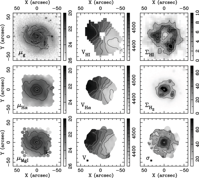
Figure 1.— Two-dimensional data used in our study of UGC 463. From top-to-bottom and left-to-right, we provide the surface brightness in AB mag arcsec^-2 for SDSS $g$-band ($\mu_{g}$), SparsePak H$\alpha$-region ($\mu_{\mbox{H$\alpha$}}$), and SparsePak$+$PPak Mg i-region ($\mu_{\mbox{\scriptsize Mg{$~{}\!$i}}}$); LOS velocity in km s^-1 for H i ($V_{\mbox{\rm\footnotesize H{i}}}$), H$\alpha$ ($V_{{\rm H}\alpha}$), and stars ($V_{\ast}$); mass surface density in $\mathcal{M}_{\odot}~{}\!$pc^-2 for H i ($\Sigma_{\mbox{\rm\footnotesize H{i}}}$) and H₂ ($\Sigma_{\rm H_{2}}$); and stellar velocity dispersion ($\sigma_{\ast}$) in km s^-1. The galaxy center, as provided by NED, is marked by either a black or white plus sign. All images have the same spatial scale and have a sky-right orientation. Contour levels are: $\mu_{{\rm H}\alpha}$ — 22, 21, 20 mag arcsec^-2; $\mu_{\mbox{\scriptsize Mg{$~{}\!$i}}}$ — 22.7, 21.7, 20.7 mag arcsec^-2; $V_{\mbox{\rm\footnotesize H{i}}}$, $V_{{\rm H}\alpha}$, $V_{\ast}$ — 4360, 4390, 4420, 4450, 4480, 4520, 4540 km s^-1; $\Sigma_{\mbox{\rm\footnotesize H{i}}}$ — 3, 6, 9 $\mathcal{M}_{\odot}~{}\!$pc^-2; $\Sigma_{\rm H_{2}}$ — 15, 30, 60 $\mathcal{M}_{\odot}~{}\!$pc^-2; and $\sigma_{\ast}$ — 30, 45, 60 km s^-1. Gray contours are used to ease visibility with respect to the background grayscale image. The contours of $\mu_{{\rm H}\alpha}$ (gray) and $\mu_{\mbox{\scriptsize Mg{$~{}\!$i}}}$ (black) are overplotted on the $\mu_{g}$ image for comparison.

2.1. Distance

The distance to UGC 463 is used to calculate: (1) the total absolute $K$-band magnitude, $M_{K}$, providing an inclination measurement via inversion of the TF relation (Section 3.1.2); and (2) the disk scale height based on a measured scale length in kpc (see equation 1 from Paper II, ). In Section 3.1.1, we find $V_{\rm sys}=4460\pm 1$ km s^-1, consistent with $V_{\rm sys}=4452\pm 9$ km s^-1 (Huchra et al., 1999) provided by NED. Applying the 104 km s^-1 flow correction (Mould et al., 2000), we calculate a flow-corrected velocity of $V_{\rm flow}=4356\pm 52$ km s^-1, where we have taken half the flow correction as its error (Paper II). Using $H_{0}=73\pm 5$ km s^-1 Mpc^-1 for Hubble’s constant (provided by NED, cf. Riess et al., 2009; Larson et al., 2011), we calculate a flow-corrected distance of $D=V_{\rm flow}/H_{0}=59.67\pm 0.01\pm 4.15$ Mpc; the systematic error is dominated by the uncertainty in $H_{0}$.

2.2. Optical and Near-Infrared Emission

We use archival $g$-, $r$-, and $i$-band data obtained from the Sloan Digital Sky Survey (SDSS; York et al., 2000) and $J$-, $H$-, and $K$-band data obtained from the Two-Micron All-Sky Survey (2MASS; Skrutskie et al., 2006) to produce surface-brightness profiles and large-aperture total magnitudes. Photometric measurements are in AB magnitudes for SDSS data and Vega-based magnitudes for 2MASS data. SDSS and 2MASS images are, respectively, $10\farcm 2\times 13\farcm 8$ and $8\farcm 3\times 17\farcm 1$ with UGC 463 well separated from the frame edges.

2.2.1 Surface Photometry

Given the basic image reduction and photometric calibration provided by SDSS and 2MASS, our surface photometry is primarily concerned with sky-background subtraction and masking sources other than UGC 463.

Source catalogs have been created for each band using Source Extractor. Each catalog has been visually inspected and pruned of erroneous source identifications, such as along meteor streaks or diffraction spikes; these features are masked from our final results by including pseudo-sources in our catalog. We have created a master catalog for the region surrounding UGC 463 by merging the catalogs from all bands, identifying sources detected in multiple bands.

Using the IRAF task imsurfit, we determine the sky background of each image by fitting a Legendre polynomial surface (with cross terms) to each image where all sources and artifacts are replaced, initially, by a ($\pm 3$) sigma-clipped mean of the image. After the lowest-order surface fit (2-$\times$2-order), masked regions are replaced by the fitted surface values as the fit order is increased. By inspection, we find there is little improvement in the sky flatness when using surfaces of more than 9-$\times$9-order (terms up to $x^{8}$), and higher order fits begin to introduce artificial structure. The backgrounds of SDSS images are generally well-behaved, whereas the 2MASS $H$- and $K$-band data exhibit significant background structure.

Surface photometry has been performed on each image after subtracting the sky background and masking all artifacts and sources, except for UGC 463. Source masking is forced to be identical in every band. From these masked images, we perform elliptical aperture photometry over a range of radii, each with an aspect ratio and orientation coinciding with the derived geometry of the disk discussed in Section 3.1. Given the shallow depth of the 2MASS data, we have also produced a $J\!H\!K$ surface-brightness profile using the unweighted sum of the $J$, $H$, and $K$ surface-brightness profiles. This extends the NIR surface-brightness profile to larger radii. The “$J\!H\!K$ bandpass” has an effective band-width of $\delta\lambda/\lambda=0.62$ and a Vega zero-point of 1062 Jy.

Table 2Exponential Disk Scale Lengths and Scale Heights

	$R_{\rm max}$	$\mu_{0}$	$h_{R}$	$h_{R}$	$q$	$h_{z}$
Band	(arcsec)	(mag arcsec-2)	(arcsec)	(kpc)	($h_{R}/h_{z}$)	(kpc)
$g$	70	$20.16\pm 0.07$	$12.0\pm 0.5$	$3.5\pm 0.1\pm 0.2$	$8.1\pm 0.3^{+2.0}_{-1.7}$	$0.43\pm 0.03^{+0.11}_{-0.08}$
$r$	70	$19.58\pm 0.06$	$12.2\pm 0.4$	$3.5\pm 0.1\pm 0.2$	$8.1\pm 0.2^{+2.0}_{-1.7}$	$0.44\pm 0.02^{+0.11}_{-0.09}$
$i$	70	$19.29\pm 0.05$	$12.6\pm 0.3$	$3.6\pm 0.1\pm 0.3$	$8.2\pm 0.2^{+2.1}_{-1.7}$	$0.44\pm 0.02^{+0.11}_{-0.09}$
$K$	55	$16.66\pm 0.09$	$11.9\pm 0.3$	$3.4\pm 0.1\pm 0.2$	$8.0\pm 0.2^{+2.0}_{-1.6}$	$0.43\pm 0.02^{+0.10}_{-0.08}$
$J\!H\!K$	80	$17.18\pm 0.05$	$12.3\pm 0.3$	$3.6\pm 0.1\pm 0.2$	$8.1\pm 0.2^{+2.0}_{-1.7}$	$0.44\pm 0.02^{+0.11}_{-0.09}$

Figure 2 provides all the surface photometry used in our present study of UGC 463. We apply Galactic extinction corrections of $A_{g}=0.357$, $A_{r}=0.242$, $A_{i}=0.173$, and $A_{K}=0.034$; no extinction correction is applied to $\mu_{J\!H\!K}$ (see Section 2.2.2). We also plot the UGC 463 $K$-band photometry from de Jong & van der Kruit (1994), which is in very good agreement with our 2MASS photometry at $R<40\arcsec$. Table 2 provides the result of fitting an exponential disk to all bands, including the $J\!H\!K$ data, demonstrating marginal change in the best-fitting scale length and no evident trend with wavelength. The Table provides the radii over which the exponential disk is fit; the minimum radius is always $15\arcsec$ in order to avoid non-exponential features seen near the galaxy center.

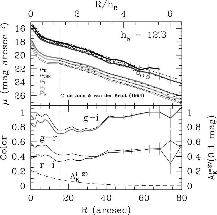
Figure 2.— Optical and NIR photometry of UGC 463, corrected for Galactic extinction; SDSS measurements are in AB magnitudes and 2MASS measurements are in Vega magnitudes. Top — From top-to-bottom, the 2MASS $K$-, combined 2MASS $J\!H\!K$-, SDSS $i$-, SDSS $r$-, and SDSS $g$-band surface-brightness profiles are plotted as solid lines; the bands are differentiated by grayscale as given by the key. Exponential-disk fits with a fixed scale length of $h_{R}=12\farcs 3$ are shown as dashed lines (compare to the results in Table 2 when $h_{R}$ is allowed to be free for each band); the vertical dotted lines marks the innermost radius included in the fit. The $K$-band data from de Jong & van der Kruit (1994) are plotted as open circles. Bottom — SDSS $g-r$, $r-i$, and $g-i$ colors; the thick gray line is the $g-i$ color after correcting for internal extinction. The estimate of the internal $K$-band extinction, $A^{i=27}_{K}$, calculated in Section 2.2.4 is also provided as a dashed line.

2.2.2 $K$-Band Surface Brightness Profile

We apply two corrections to $\mu_{J\!H\!K}$ and use it as the primary NIR surface-brightness measurement for our study of UGC 463: (1) a color correction to produce a more accurate $K$-band surface-brightness profile at large radius and (2) an instrumental-smoothing correction. The color correction compares $\mu_{K}$ and $\mu_{J\!H\!K}$ from Figure 2, such that it includes the Galactic extinction correction to $\mu_{J\!H\!K}$. We find $\mu_{K}-\mu_{J\!H\!K}=-0.47\pm 0.03$ at $R<40\arcsec$ with a maximum deviation from the mean of 0.05 magnitudes, which is at most $\sim\epsilon(\mu_{K})$. The NIR color gradients are small over this radius, with $\Delta(J-H)\lesssim 0.2$ and $\Delta(J-K)\lesssim 0.1$, and roughly consistent with no color gradient to within the photometric error.

Our instrumental-smoothing correction effectively performs a one-dimensional bulge-disk decomposition of $\mu_{J\!H\!K}$. We assume the central light concentration intrinsically follows a Sérsic (1963) profile. After first subtracting an exponential surface-brightness profile fitted to $\mu_{J\!H\!K}$ data between $10\arcsec<R<33\arcsec$, we model the central light concentration within $R<8\arcsec$ by a Sérsic profile convolved with a Gaussian kernel, assuming the latter is a good approximation for all instrumental effects. We find a best-fitting Sérsic index of $n=1.5$ and an effective (half-light) radius of $R_{e}=1\farcs 7$. Random errors in this modeling are approximated by the root-mean-square (RMS) difference between the measured and modeled central light profile. We assume that the “intrinsic disk surface brightness” is the remainder of the profile after subtracting the model of the central-light concentration, the “intrinsic central light concentration” is the Sérsic component of the model, and the “intrinsic $\mu_{J\!H\!K}$ profile” is the sum of these two components; our instrumental-smoothing correction then consists of the difference between the measured and “intrinsic” $\mu_{J\!H\!K}$ profile. We adopt a conservative 50% systematic error in this correction due to the inherent uncertainties in the true parameterization of the central light concentration and instrumental-smoothing kernel. Although relevant to our assessment of any central mass concentration in our calculations of $\Sigma_{\rm dyn}$ (Section 5.3), $\Upsilon_{\ast,K}^{\rm disk}$ (Section 5.6), and the mass budget (Section 6), our instrumental-smoothing correction is immaterial to the fundamental conclusions of our paper.

Hereafter, we refer to the corrected $J\!H\!K$ measurement as $\mu^{\prime}_{K}$; $h_{R}$ always refers to the measurement based on this profile unless otherwise stated. The fully corrected $\mu^{\prime}_{K}$ profile is shown in, e.g., Figure 4.

2.2.3 Total Apparent $K$-Band Magnitude

In Section 3.1.2, we use $M_{K}$ to calculate the inverse-TF inclination of UGC 463 based on the TF relations derived by V01. Therefore, we calculate the total apparent magnitude, $m_{K}$, using the 2MASS $K$-band data according to the procedure used by V01: We measure a roughly isophotal magnitude at $\mu_{K}=21.5$ mag arcsec^-2 (the rough surface-brightness limit occurring at $R\lesssim 55\arcsec$) and extrapolate to infinity based on the fitted exponential disk ($h_{R}=12\farcs 3\pm 0\farcs 3$). We find $m_{K}(R\leq 55\arcsec)=9.45\pm 0.01$ and a correction of -0.09 mag for the extrapolation of the disk. Accounting for Galactic-extinction ($A_{K}=0.034$), we find $m_{K}=9.32\pm 0.02$.

2.2.4 Internal Dust Extinction

Left uncorrected, $\mu^{\prime}_{K}$ may overestimate our dynamical mass-to-light ratios (Section 5.6) due to internal dust extinction in $K$-band, $A^{i}_{K}$. Using the dust-slab model from Tully & Fouque (1985) and $i=27\arcdeg\pm 2\arcdeg$ (Section 3.1), we calculate the function $A^{i=27}_{K}(R)$ as shown in Figure 2, which has a maximum of $A^{i=27}_{K}(R=0)=0.02\pm 0.01$ at the galaxy center. Assuming $A_{V}/E(B-V)=3.1$ (Cardelli et al., 1989), we calculate $A_{K}/E(g-i)=0.18\pm 0.02$, which we use to apply an internal reddening correction to our $g-i$ color when comparing our dynamical $\Upsilon_{\ast}$ measurements to those predicted by SPS modeling. Figure 2 plots the uncorrected $g-r$, $r-i$, and $g-i$ colors, as well as our internal-reddening-corrected $(g-i)_{0}$ color. Compared to more realistic radiative-transfer modeling including a clumpy ISM and spiral structure, these simple dust-slab model predictions tend to overestimate both the level of dust extinction and reddening toward high inclination; the predictions are more reasonable at the low inclination appropriate for UGC 463 (Schechtman-Rook et al., in prep). Given the marginal extinction in $K$-band and reddening of $g-i$, the simpler model is sufficient for our purposes.

2.2.5 Dust Emission

We note here that the $K$-band also contains emission from hot dust and polycyclic aromatic hydrocarbons; however, based on a preliminary modeling of the spectral energy distribution of our full suite of NIR and Spitzer imaging, we expect this to be no more than a 3% contribution, which is immaterial to the conclusions of this paper.

2.3. Ionized-Gas Kinematics

We primarily use ionized-gas kinematics obtained by the SparsePak (Bershady et al., 2004, 2005) and PPak (Verheijen et al., 2004; Roth et al., 2005; Kelz et al., 2006) integral-field units (IFUs), augmented by our H i observations, to produce the total rotation curve of UGC 463. These ionized-gas data also provide measurements of the gas velocity dispersion, which we use to correct the gas rotation speed to the circular speed (Section 4.3.1). Below, we briefly describe the IFU data available for UGC 463 and our extraction of the ionized-gas kinematics.

2.3.1 H$\alpha$, N ii, & S ii Spectroscopy

SparsePak integral-field spectroscopy (IFS) of UGC 463 was obtained on the nights of UT 02 January 2002 and UT 20 October 2002, following the setup provided for the H$\alpha$ region as listed in Table 1 of Paper I. We obtained four pointings during the January run and an additional three pointings during the October run. The pointings nominally followed the 3-pointing dither pattern designed to fully sample the $72\arcsec\times 71\arcsec$ FOV of SparsePak (Bershady et al., 2004); the fourth pointing during the January 2002 run was a repeat of the center pointing. We obtained 2$\times$15-minute exposures for each pointing. Each exposure pair is combined, before extraction of the spectra, while simultaneously removing cosmic rays. Spatially overlapping fibers among the seven pointings are not combined but treated individually throughout our analysis. Further details of the reduction of these data (basic image reduction, spectral extraction, wavelength calibration, and sky and continuum subtraction) are provided by Swaters et al., in prep, largely following methods described in Andersen et al. (2006) with continuum-subtraction techniques described in Bershady et al. (2005). The RMS difference between the catalogued and measured line centroids for the ThAr lines used in our wavelength calibration, i.e. the “wavelength calibration error,” is typically $\lesssim 0.1$ km s^-1.

We also measure the instrumental dispersion, $\sigma_{\rm inst}$, as a function of wavelength for all spectra, using the ThAr emission lines from our calibration lamp spectra (Paper II). The intrinsic widths of the ThAr features are negligible such that the second moment of these lines is equivalent to $\sigma_{\rm inst}$ to good approximation. After identifying a set of appropriate (unblended) lines from the calibration spectrum, we fit single Gaussian functions to each line using the same code described by Andersen et al. (2008) to fit the emission-line features in our galaxy spectra (see also Swaters et al., in prep). For each fiber, we fit a quadratic Legendre polynomial to $\sigma_{\rm inst}(\lambda)$, which is used to interpolate $\sigma_{\rm inst}$ at any wavelength. The average instrumental broadening across the full spectral range for all fibers is 13 km s^-1.

2.3.2 O iii Spectroscopy

Our optical continuum spectra in the Mg i region taken with both SparsePak and PPak — described in Sections 2.4.1 and 2.4.2, respectively — have sufficient spectral range to include the [O iii]$\lambda$5007 emission feature. Therefore, we also use these lines as tracers of the ionized-gas kinematics. No adjustment of the continuum-data reduction recipe was needed to accommodate the proper handling of the emission features. Instrumental dispersions are calculated as described in Sections 2.4.1 and 2.4.2 for the SparsePak and PPak data, respectively.

2.3.3 Kinematic Measurements

Ionized-gas kinematics are measured for all available emission lines. Following Andersen et al. (2008, see also ), both single and double Gaussian line profiles are fitted in a 20Å window centered around each line. All Gaussian fits have been visually inspected to ensure each emission line was fitted properly. Velocities ($cz$) of each atomic species are calculated separately using the wavelength of the Gaussian centroid. Of all fitted line profiles, 27% are better fit by a double Gaussian profile (Andersen et al., 2008, Andersen et al., in prep); in these cases, a single component is used to measure the line-of-sight (LOS) velocity. Ionized-gas velocity dispersions, $\sigma_{\rm gas}$, also use a single component and are corrected for the measured instrumental line width.

For our H$\alpha$-region spectroscopy, we combine all available velocity and velocity dispersion measurements (any combination of the [N ii]$\lambda$6548, H$\alpha$, [N ii]$\lambda$6583, [S ii]$\lambda$6716, and [S ii]$\lambda$6731 lines) into an error-weighted mean velocity for each fiber. Due to the large uncertainties in $\sigma_{\rm gas}$ for lines other than H$\alpha$, we only include measurements with $\epsilon(\sigma_{\rm gas})<3$ km s^-1 in the combined value. In this spectral region, both velocities and $\sigma_{\rm gas}$ are dominated by the H$\alpha$ line measurements due to the higher $S/N$ of these lines; hereafter, we refer to these kinematics as “H$\alpha$” kinematics, despite their inclusion of other ionized atomic species.

In addition to the consistency check among measurements made by SparsePak and PPak, the [O iii] kinematics provide a useful comparison with the H$\alpha$ results (see Section 4). However, the H$\alpha$ line generally provides higher quality kinematics and velocity fields: the line $S/N$ is higher on average and the filling factor of the kinematic measurements in the disk of UGC 463 is more uniform. We eventually combine all ionized-gas kinematics into a single, axisymmetric set of measurements (Section 4.3); however, it is useful to keep in mind this distinction between the merit of the H$\alpha$ and [O iii] kinematic data.

2.4. Stellar Kinematics

Our optical continuum spectra are at the heart of this paper and, in fact, our entire survey. UGC 463 is among a set of 19 galaxies in (and roughly half of) our Phase-B sample that have both SparsePak and PPak continuum spectroscopy near the Mg i triplet. This intentional duplication provides an internal consistency check of our stellar kinematics using two different instruments, and we find excellent agreement among the observations (Section 4). Here, we provide information concerning our observations and our derivation of the LOS stellar kinematics.

2.4.1 SparsePak Spectroscopy

SparsePak IFS of UGC 463 was obtained using the Mg i-region setup as listed in Table 1 of Paper I — primarily targeting Fe i and Mg i stellar-atmospheric absorption lines. The observation and reduction of these data are described by Westfall (2009); we review the salient details here.

UGC 463 was observed on consecutive nights during a single run from UT $23-25$ September 2006. Four, six, and four 45-minute exposures were taken during the three nights of observation, respectively. No dithering of the pointing was applied between exposures; the original pointing was repeated to the best of our ability for each night. Exposures taken within a given night have been combined into a single image, using an algorithm that simultaneously rejects cosmic rays, and reduced (basic image reduction, spectral extraction, wavelength calibration, and sky-subtraction) on a night-by-night basis. The basic reduction procedures are nearly the same as that used for the H$\alpha$ data (Section 2.3.1). The wavelength calibration errors are typically $\lesssim 0.1$ km s^-1. Error spectra have been calculated in a robust and parallel analysis. The repeatability of the pointing across the three nights of observation was good to less than one arcsecond, determined by Westfall (2009) by forcing the kinematic centers of all the SparsePak H$\alpha$ and [O iii] data to follow from the same on-sky kinematic geometry. Thus, the extracted spectra from each night have been combined on a fiber-by-fiber basis and weighted by the spectral $(S/N)^{2}$. The weighting is relevant due to changing conditions; moon illumination increased for each night (from $1-7$%) and a number of exposures ($\sim 30$%) suffered from variable transparency losses due to passing clouds, particularly during the second night of observation. The combined spectra, from all 10.5 hours of integration, are analyzed in Section 2.4.3 to measure stellar kinematics for UGC 463.

Using our calculated error spectra, Figure 3 plots the mean $S/N$ of our SparsePak IFS as a function of radius against the $g$-band surface-brightness profile, demonstrating that we have measured stellar kinematics for fibers with $\mu_{g}\sim 22.5$ at $S/N\sim 3$. The scale translation between mean $S/N$ and $\mu_{g}$ assumes the data are detector-limited ($S/N\propto$ flux), which is only an approximation for our data.

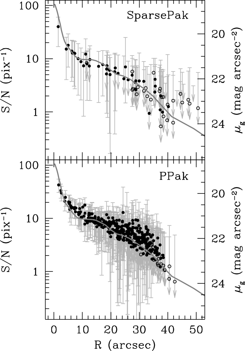
Figure 3.— Mean $S/N$ measurements for both our SparsePak (top) and PPak (bottom) Mg i-region IFS of UGC 463. Data are plotted as a function of radius and against the SDSS $g$-band profile (gray line; Section 2.2.1). Bars provide the range in $S/N$ of all pixels over the full spectrum; upper limit arrows are used in cases where $S/N$ drops below zero due to the random errors in sky subtraction. Spectra that have yielded stellar kinematics are plotted by filled points and as open circles otherwise.

Finally, we estimate $\sigma_{\rm inst}$ for both the template and galaxy spectra for use in measuring instrumental-broadening corrections (Section 2.4.4). We use the same approach as described for the H$\alpha$-region spectroscopy in Section 2.3.1 for both the galaxy and template observations. The average instrumental broadening for these galaxy spectra is 11 km s^-1.

2.4.2 PPak Spectroscopy

PPak IFS of UGC 463 was obtained using the Mg i-region setup as listed in Table 1 of Paper I. Compared to the SparsePak optical continuum spectra, individual PPak spectra have approximately 1.5 times the spectral range, 0.7 times the spectral resolution, and 0.6 times the on-sky aperture per fiber; however, PPak contains 4.4 times as many fibers as SparsePak in its main fiber bundle. These data are described by Martinsson (2011), which includes all Mg i-region data taken by PPak. Here, we briefly review the acquisition and reduction of the data specifically for UGC 463.

We obtained two consecutive 1-hour exposures targeting UGC 463 on each of three nights from UT $13-15$ November 2004, yielding six hours of total on-target integration. Flexure corrections have been applied on an exposure-by-exposure basis, requiring spectral extraction, wavelength calibration, and sky subtraction to be performed on each exposure individually. The RMS wavelength calibration error is typically of the same order as that found for the SparsePak observations ($\sim 0.1$ km s^-1). Error spectra have been calculated in a robust and parallel analysis. For UGC 463, no pointing offsets were detected; the CCD of the guide camera of the PMAS spectrograph allows for accurate reacquisition of our target galaxies on subsequent nights. All six spectra for a given fiber have been combined using weights depending on the instrumental resolution and the spectral $S/N$ as described by Martinsson (2011).

Figure 3 provides the mean $S/N$ of the PPak spectra, alongside that of the SparsePak spectra. Despite the shorter integration time and smaller fiber aperture, the PPak data have slightly higher mean $S/N$, an effect of both the lower spectral resolution and the better efficiency of PMAS over the WIYN Bench Spectrograph.

Instrumental broadening measurements are performed differently for PPak data than described above for SparsePak data. PPak observations provide simultaneous calibration spectra in 15 fibers, evenly distributed along the pseudo-slit among the galaxy spectra. These spectra have proven critical for applying the necessary flexure corrections (Martinsson, 2011). Moreover, they provide simultaneous measurements of the instrumental dispersion, obtained by fitting Gaussian functions to the ThAr emission lines. Martinsson (2011) has fit a quadratic Legendre polynomial surface to these measurements of $\sigma_{\rm inst}$ for each object frame. We use this description of $\sigma_{\rm inst}$ to calculate the instrumental-dispersion corrections for both the ionized-gas and stellar kinematics measured from the PPak spectra. The mean instrumental dispersion across all fibers and all spectral channels is 17 km s^-1 for our PPak data of UGC 463.

2.4.3 Raw Kinematic Measurements

We use the Detector-Censored Cross-Correlation (DC3) software presented in Westfall et al. (2011, hereafter Paper III) to determine spatially resolved stellar kinematics in UGC 463 from both our SparsePak and PPak spectra. Based on a preliminary analysis (Paper II), we find a K1 III star provides a minimum template-mismatch error of $\sim 5$% in the observed velocity dispersion ($\sigma_{\rm obs}$) with no systematic trend in radius. In the future, we can improve upon this by using composite templates; however, a 5% template-mismatch error in $\sigma_{\rm obs}$ is satisfactory for the present study.

As per our survey protocol (Paper I), we have observed template stars in the Mg i region using both SparsePak and PPak. For the analysis here, we specifically use the K1 III stars HD 167042 and HD 162555 for our SparsePak and PPak stellar kinematics, respectively; Table 3 presents salient information regarding the template spectra. Template star observations are performed under nominally the same spectrograph/telescope configuration as for our galaxy data. For both SparsePak and PPak, template stars are observed by drifting the star through the full FOV, yielding many spectra that are combined to provide high-$S/N$ templates; the final $S/N$ of each template is provided in Table 3.

Table 3Stellar Templates

					Physical Quantities
	Spectral			$S/N$	$V_{\rm hel}$	$T_{\rm eff}$	$\log g$	[Fe/H]
HD	Type	Instrument	UT Date	(pix-1)	(km s-1)	(K)	(cm s-2)	(dex)
167042	K1 III	SparsePak	2001-06-09	0.4$\times 10^{3}$	$-18.01\pm 0.17$	4878	2.74	-0.11
162555	K1 III	PPak	2007-01-15	1.1$\times 10^{3}$	$-14.84\pm 0.20$	4660	2.72	-0.21

We fit any galaxy–template cross-correlation (CC) function that peaks within a few hundred km s^-1 of the systemic velocity of UGC 463 (as recorded by NED) regardless of the $S/N$. For each fiber, we adopt a Gaussian broadening function, and we use a cubic Legendre polynomial to minimize continuum differences between the broadened template and the fitted galaxy spectrum. Additionally, we mask the [O iii]$\lambda$5007 and [N i] ($\lambda$5198 and $\lambda$5200) nebular emission regions from both the template and galaxy spectra. For the PPak data, the redshifted [O iii]$\lambda$4960 line is also visible; however, DC3 masks the CC to a rest-wavelength range common to both the galaxy and template spectrum, thereby automatically masking this line. Each CC fit has been visually inspected to insure the proper peak was considered by the fitting algorithm and that any unexpected artifacts — poorly removed sky lines and/or cosmic-ray detections — were masked. Based on this inspection, spectra have been refit as necessary. Our stellar kinematic analysis follows the expectations derived for random errors in Paper III. As assessed via $\chi^{2}$ and the velocity shift with respect to spatially neighboring fibers, we find reasonable fits to spectra with mean $S/N$ approaching unity, albeit with large errors. Systematic errors should be negligible for velocity measurements at all $S/N$, and they should be $\lesssim 20$% in $\sigma_{\rm obs}$ at $S/N\gtrsim 2$; systematic errors are always smaller than the calculated random error (Paper III).

2.4.4 Instrumental-broadening Corrections

We correct our observed stellar kinematics for the system response function by considering the following two separable components: (1) The broadening of the intrinsic absorption-line widths due to the spectrograph optics, accounted for using an “instrumental-broadening” correction, $\delta\sigma_{\rm inst}$; and (2) The smearing of the intrinsic surface-brightness, velocity, and velocity dispersion distributions by the response of the atmosphere$+$telescope system, accounted for using a “beam-smearing” correction, $\sigma_{\rm beam}$. The final LOS dispersion is $\sigma_{\ast}^{2}=\sigma_{\rm obs}^{2}-\delta\sigma_{\rm inst}^{2}-\sigma_{\rm beam}^{2}$ (Paper II). Unlike $\sigma_{\rm beam}$, $\delta\sigma_{\rm inst}$ is independent of the on-sky geometry and intrinsic kinematic structure of the observed galaxy; therefore, we calculate $\delta\sigma_{\rm inst}$ here. We calculate $\sigma_{\rm beam}$ before combining our SparsePak and PPak kinematics in Section 4 using the projection geometry derived in Section 3.

Each CC is used to compare template and galaxy absorption-line shapes such that $\delta\sigma_{\rm inst}$ is determined by the difference in $\sigma_{\rm inst}$ measured for the template and galaxy spectrum; we calculate $\delta\sigma_{\rm inst}$ following Appendix A of Paper III using our measurements of $\sigma_{\rm inst}$ for both the template and galaxy spectra. We adopt a 4% error in $\delta\sigma_{\rm inst}$ (Paper II), which is marginal when compared to $\epsilon(\sigma_{\rm obs})$. These corrections differ rather dramatically between SparsePak and PPak; however, in both cases, $\delta\sigma_{\rm inst}^{2}$ is typically small. Corrections to $\sigma_{\rm obs}$ — i.e., the ratio $(\sigma_{\rm obs}^{2}-\delta\sigma_{\rm inst}^{2})^{\frac{1}{2}}/\sigma_{\rm obs}$ — are $\lesssim 4$% and $\lesssim 20$% for, respectively, 90% and 99% of all measurements; a few measurements have rather large corrections due to dispersion measurements of $\sigma_{\rm obs}<10$ km s^-1, which are likely erroneously low (Paper III). We always find $\delta\sigma_{\rm inst}<\epsilon(\sigma_{\rm inst})$.

2.5. Atomic-Gas Content

As part of our general survey strategy (Paper I), we have obtained 21cm aperture-synthesis imaging for the DMS Phase-B sample. These data measure neutral hydrogen (H i) surface densities ($\Sigma_{\mbox{\rm\footnotesize H{i}}}$) and extend the rotation-curve measurements of each galaxy; the ionized-gas kinematics can be limited by the FOV of our H$\alpha$ spectroscopy and/or the extent of the H$\alpha$ emission in the disk. For UGC 463, we obtained 2.3 hours of on-source integration using the Very Large Array (VLA); observations were taken in the C configuration yielding a synthesized beam of $14\farcs 7\times 12\farcs 9$ and a velocity resolution of 10.5 km s^-1. In the end, these data provide only a marginal radial extension of the ionized-gas rotation curve of UGC 463. The acquisition and reduction of these data is fully described by Martinsson (2011).

The two-dimensional H i mass-surface-density map and velocity field are presented in Figure 1. The azimuthally averaged measurements of $\Sigma_{\mbox{\rm\footnotesize H{i}}}(R)$ for UGC 463 are presented in Figure 4; we adopt $\epsilon(\Sigma_{\mbox{\rm\footnotesize H{i}}})=0.1\Sigma_{\mbox{\rm\footnotesize H{i}}}$. As is typical of late-type spiral galaxies we find a decrease in the H i mass surface density toward the galaxy center; the peak surface density of $\Sigma_{\mbox{\rm\footnotesize H{i}}}=5.6$ $\mathcal{M}_{\odot}~{}\!$pc^-2 occurs at $R=1.9h_{R}$. Although the spatial resolution of our H i column-density map is a factor of $\gtrsim 3$ larger than our optical IFU data, we do not attempt to match the resolution of these two data sets; such a correction to the azimuthally averaged total mass surface density is negligible for the purposes of this paper.

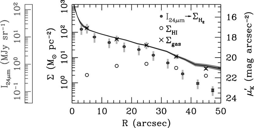
Figure 4.— Mass surface density measurements for H i (via direct observation; open circles) and H₂ (via an indirect calculation; gray-filled points), and all gas including helium and metals (crosses). The gray-filled points also provide the $I_{24\mu{\rm m}}$ profile as delineated by the ordinate to the far left. Errors (random in black and systematic in gray) shown for $\Sigma_{\rm H_{2}}$ and $\Sigma_{\rm gas}$ are discussed in the text; errors in $\Sigma_{\mbox{\rm\footnotesize H{i}}}$ are of order the size of the plotted symbol. As delineated by the right ordinate, we overplot $\mu^{\prime}_{K}$ (Section 2.2.2) as the solid line with the error region plotted in dark gray.

2.6. Molecular-Gas Content

Our nominal survey scope does not include direct observations of the molecular content of our galaxy sample via, e.g., the ¹²CO ($J=1\rightarrow 0$) emission line — henceforth all discussion of “CO emission” refers to this emission feature unless noted otherwise. Until we obtain such data, estimation of the molecular content in DMS galaxies relies on available literature data and/or inference from other suitable tracers for which data is available.

For our characterization of the molecular content of UGC 463, we use our 24$\mu$m Spitzer imaging to produce a rough approximation of the CO surface-brightness distribution. Numerous studies exist demonstrating a correlation between the infrared luminosity of star-forming galaxies (dominated by thermal dust emission) and their molecular-gas content as traced by CO emission. For example, the integrated infrared luminosity based on IRAS observations is well-correlated with the integrated CO flux (Young & Scoville, 1991). Moreover, Bendo et al. (2007) note a similar dependence of the distribution of 24$\mu$m emission on morphological type as was noted by Young et al. (1995) for the molecular gas traced by CO emission. At spatially resolved scales, Paladino et al. (2006) have studied the correlation between CO ($I_{\rm CO}\Delta V$) and 24$\mu$m emission ($I_{24\mu{\rm m}}$) in a set of 6 nearby spiral galaxies to find $I_{24\mu{\rm m}}\propto(I_{\rm CO}\Delta V)^{0.9\pm 0.1}$. Correlations between the CO and 8$\mu$m emission have also been discussed (Regan et al., 2006; Bendo et al., 2010); however, we prefer to focus on the correlation between $I_{\rm CO}\Delta V$ and $I_{24\mu{\rm m}}$ as the latter should be dominated by warm dust emission and be less dependent on the fraction of dust in the form of polycyclic aromatic hydrocarbons (see, e.g., Draine & Li, 2007).

In Section 2.6.1, we describe the procedure used to measure $I_{24\mu{\rm m}}(R)$ in UGC 463. In Section 2.6.2, we detail the calibration of our $I_{24\mu{\rm m}}$-to-$I_{\rm CO}\Delta V$ surface-brightness relation using data made available by Leroy et al. (2008, hereafter L08). Finally, in Section 2.6.3, we convert from $I_{24\mu{\rm m}}$ to $I_{\rm CO}\Delta V$ and then calculate the molecular mass surface density, $\Sigma_{\rm H_{2}}$, using the traditional $X$-factor, $X_{\rm CO}$. This latter step dominates the systematic error in our estimation of the molecular content of UGC 463.

2.6.1 24$\mu$m Spitzer Photometry

The survey strategy for all our Spitzer observations are provided in Section 6.2.3 of Paper I. In general, 24$\mu$m images collected for the DMS demonstrate significant background structure, due to both detector effects and intrinsic structure in the Galactic ISM, with fluctuations on angular scales close to that of our galaxies. To account for these fluctuations, we mask out all statistically significant sources, including a substantial radial region surrounding UGC 463, and create a $47\arcsec\times 47\arcsec$ boxcar-smoothed background image. Masked regions are iteratively filled by the boxcar smoothing, effectively interpolating the sky background and its gross structure, across all detected sources. We simply subtract this smoothed image from our 24$\mu$m image of UGC 463 and use the result to calculate the 24$\mu$m surface-brightness profile.

Our background-subtraction procedure has been carefully assessed to ensure that the low-surface-brightness extent of UGC 463 has not been systematically over-subtracted. Preliminary tests with UGC 463 and other galaxies in our survey demonstrate that our $I_{24\mu{\rm m}}$ profiles become strongly affected by the sky-subtraction errors at a source intensity below $I_{24\mu{\rm m}}<0.05$ MJy sr^-1 ($\Sigma_{\rm H_{2}}<0.21$ $\mathcal{M}_{\odot}~{}\!$pc^-2 in Figure 4). UGC 463 is the third brightest 24$\mu$m emitter in our entire sample, meaning that this surface brightness limit falls outside the radial region relevant to this paper. Our measured 24$\mu$m surface-brightness profile uses elliptical apertures following a geometry identical to that used for the optical and NIR photometry in Section 2.2.1. Figure 4 provides the 24$\mu$m surface-brightness profile and the result of its conversion to $\Sigma_{\rm H_{2}}$, according to the discussion in the next two sections. The random errors in our $I_{24\mu{\rm m}}$ measurements incorporate a constant 4% calibration error (Engelbracht et al., 2007) and a sky-subtraction error estimated by the change in $I_{24\mu{\rm m}}$ introduced by a factor of two change in the smoothing-box size; the latter results in 1% and 10% sky-subtraction errors at $R\sim 30\arcsec$ and $\sim 47\arcsec$, respectively.

2.6.2 24$\mu$m-to-CO Surface Brightness Calibration

We use measurements of both CO and 24$\mu$m emission provided by L08 (see their Table 7) to measure the correlation between $I_{24\mu{\rm m}}$ and $I_{\rm CO}\Delta V$. Twelve of the 23 galaxies studied by L08 include both CO and 24$\mu$m observations; however, four of those galaxies (NGC 2841, NGC 3627, NGC 4736, and NGC 5194) are listed in NED as having either LINER or Seyfert activity, unlike UGC 463. Therefore, we calibrate $I_{24\mu{\rm m}}/I_{\rm CO}\Delta V$ using only the remaining eight galaxies, hereafter the “$I_{24\mu{\rm m}}/I_{\rm CO}\Delta V$ subsample.”

The quantities provided by L08 are matched-resolution, azimuthally averaged radial profiles of $\Sigma_{\rm H_{2}}$ (based on CO emission and a value for $X_{\rm CO}$) and the contribution of embedded star formation (determined from the 24$\mu$m surface brightness) to the total star-formation-rate surface density. We revert these quantities to $I_{\rm CO}\Delta V$ (in K km s^-1) and $I_{24\mu{\rm m}}$ (in MJy sr^-1) using equations A2 and D1 from L08. All eight galaxies in the $I_{24\mu{\rm m}}/I_{\rm CO}\Delta V$ subsample were observed as part of the HERACLES Survey (Leroy et al., 2009), observing only the ¹²CO($J=2\rightarrow 1$) emission line, where L08 adopt a line ratio of ¹²CO($J=2\rightarrow 1$)/¹²CO($J=1\rightarrow 0$) = 0.8. The CO surface brightness has been determined by integrating the emission profile over the full line width and converting the flux units per beam to Kelvin using the Rayleigh-Jeans limit. The 24$\mu$m fluxes are determined from surface photometry of Spitzer imaging data obtained by the SINGS Survey (Kennicutt et al., 2003).

Figure 5 presents the data for the $I_{24\mu{\rm m}}/I_{\rm CO}\Delta V$ subsample regardless of the galaxy or radial region from which it has been measured. Table 7 from L08 is used to calculate $\epsilon(I_{\rm CO}\Delta V)$ directly, whereas we adopt a uniform $\epsilon(I_{24\mu{\rm m}})=0.15I_{24\mu{\rm m}}$ due to insufficient information; we expect this $\epsilon(I_{24\mu{\rm m}})$ to be an upper limit. We fit a power-law relationship between $I_{24\mu{\rm m}}$ and $I_{\rm CO}\Delta V$ to all available data, incorporating errors in both coordinates (Section 15.3 of Press et al., 2007), finding a best fit of

$$\log\left[\frac{I_{\rm CO}\Delta V}{\rm K\ km\ s^{-1}}\right]=\left(1.08\ \log\left[\frac{I_{24\mu{\rm m}}}{\rm MJy\ sr^{-1}}\right]+0.15\right),$$ (1)

with a weighted standard deviation of $\pm 0.11$ dex, in good agreement with the previous result from Paladino et al. (2006). Thus, given that UGC 463 has physical parameters that are comparable to the $I_{24\mu{\rm m}}/I_{\rm CO}\Delta V$ subsample, our calibration is expected to estimate $I_{\rm CO}\Delta V$ for this galaxy to within $\sim 30$%.

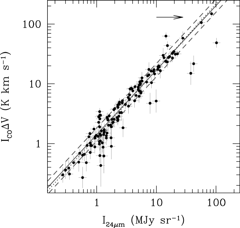
Figure 5.— Correlation between azimuthally averaged values of the 24$\mu$m and CO surface brightness from L08 for the $I_{24\mu{\rm m}}/I_{\rm CO}\Delta V$ subsample (see text). The best-fit linear correlation (equation 1) is given by the solid line; the dashed lines illustrate the weighted standard deviation about the fit. The dotted line has the slope determined by Paladino et al. (2006) using a different galaxy sample with different CO data. The arrow at the top of the plot indicates the peak $I_{24\mu{\rm m}}$ measured for UGC 463.

2.6.3 H₂ Mass Surface Density

Using equation 1, we convert our sky-subtracted 24$\mu$m image of UGC 463 to a CO surface brightness map. Subsequently, we calculate the H₂ mass surface density using the traditional conversion factor, $X_{\rm CO}$, following

$$\left[\frac{\Sigma_{\rm H_{2}}}{\mathcal{M}_{\odot}\ {\rm pc}^{-2}}\right] = 1.6\left[\frac{I_{\rm CO}\Delta V}{\rm K\ km\ s^{-1}}\right]\times$$ (2)

$$\left[\frac{X_{\rm CO}}{\rm 10^{20}\ cm^{-2}\ (K\ km\ s^{-1})^{-1}}\right]\cos i,$$

where $i$ is the galaxy inclination and $X_{\rm CO}$ is the ratio of the H₂ column density to the CO line strength. This use of $X_{\rm CO}$ to calculate $\Sigma_{\rm H_{2}}$ is a common procedure for calculating the molecular-gas content of external galaxies; however, it may suffer from substantial systematic error.

A large number of studies have been devoted to measuring $X_{\rm CO}$ both in our own Galaxy and within the Local Group. Empirical and theoretical studies suggest $X_{\rm CO}$ likely depends on multiple physical parameters, such as metallicity, radiation field, gas mass surface density, and density structure (Arimoto et al., 1996; Mihos et al., 1999; Boselli et al., 2002; Bell et al., 2006; Narayanan et al., 2011). Moreover, direct measurement of $X_{\rm CO}$ is observationally challenging: For example, the assumption of virial equilibrium and the finite spatial resolution of giant molecular clouds, in even Local Group galaxies, may both lead to inflated values of $X_{\rm CO}$ (Blitz et al., 2007; Bolatto et al., 2008); see Bolatto et al. (2008) for a more general review of $X_{\rm CO}$ measurements. Keeping these complications in mind, our analysis here adopts a simple approach: Combining the Galactic measurement of $X_{\rm CO}=1.8\pm 0.3$ from Dame et al. (2001) with the measurements for M31 ($X_{\rm CO}=3.6\pm 0.3$) and M33 ($X_{\rm CO}=2.6\pm 0.4$) from Bolatto et al. (2008), we find a mean and range of $X_{\rm CO}=(2.7\pm 0.9)\times 10^{20}$ cm^-2 (K km s^-1)^-1. We assume this value to be representative of UGC 463, given that the Milky Way, M31 and M33 are arguably the only spiral galaxies with well-resolved observations of giant molecular clouds or associations from which robust measurements of $X_{\rm CO}$ can be made.

Figure 1 provides the 24$\mu$m image, converted to $\Sigma_{\rm H_{2}}$ in units of $\mathcal{M}_{\odot}\ {\rm pc}^{-2}$ using the $I_{24\mu{\rm m}}/I_{\rm CO}\Delta V$ calibration from Section 2.6.2 and assuming $X_{\rm CO}=2.7\times 10^{20}$ cm^-2 (K km s^-1)^-1. Figure 4 provides the azimuthally averaged surface density profile $\Sigma_{\rm H_{2}}(R)$ using the 24$\mu$m surface-brightness profile from Section 2.6.1. Errors in $\Sigma_{\rm H_{2}}$ are plotted separately for random and systematic components; the former includes errors from the $I_{24\mu{\rm m}}$ calibration and photometry and the inclination, whereas the latter includes the $I_{24\mu{\rm m}}/I_{\rm CO}\Delta V$ calibration error and range in $X_{\rm CO}$. This estimate of $\Sigma_{\rm H_{2}}(R)$ agrees with the expectation that H₂ is concentrated toward the “hole” in the H i mass surface density, also seen in Figure 1 and studies of other galaxies (e.g., L08, ).

Out to 15 kpc (4.2 $h_{R}$), we find $\mathcal{M}_{\mbox{H${}_{2}$}}/\mathcal{M}_{\mbox{H{$~{}\!$i}}}=3.2$, a value that is reasonable with respect to direct CO and H i studies in the literature. In particular, Young & Knezek (1989) find a range of 0.2 and 4.0 for, respectively, late- and early-type spiral galaxies, comparable to the range measured by the more recent COLD GASS survey (Saintonge et al., 2011). However, despite having a total $\mathcal{M}_{\mbox{H${}_{2}$}}/\mathcal{M}_{\mbox{H{$~{}\!$i}}}$ that is decreased by $\sim 10$% compared to the measurement within 15 kpc (Martinsson, 2011), UGC 463 is more rich in molecular gas than the mean $\mathcal{M}_{\mbox{H${}_{2}$}}/\mathcal{M}_{\mbox{H{$~{}\!$i}}}$ calculated by Saintonge et al. (2011) for the COLD GASS survey by approximately twice the standard deviation. Similarly, by combining our 24$\mu$m imaging, the $I_{24\mu{\rm m}}/I_{\rm CO}\Delta V$ and $X_{\rm CO}$ values derived herein, and the H i data presented by Martinsson (2011) for 24 galaxies in the DMS, we find a mean of $\mathcal{M}_{\mbox{H${}_{2}$}}/\mathcal{M}_{\mbox{H{$~{}\!$i}}}=0.48$, consistent with the Saintonge et al. (2011) measurement after accounting for the difference in their adopted $X_{\rm CO}$; UGC 463 has the maximum value of $\mathcal{M}_{\mbox{H${}_{2}$}}/\mathcal{M}_{\mbox{H{$~{}\!$i}}}$ and 21 of 24 galaxies have $\mathcal{M}_{\mbox{H${}_{2}$}}/\mathcal{M}_{\mbox{H{$~{}\!$i}}}<1$. Therefore, consideration of the molecular mass component in UGC 463 is relatively more important to our dynamical $\Upsilon_{\ast}$ measurements and the baryonic mass budget than the majority of galaxies in the DMS. In Section 5.6, we discuss both the total dynamical mass-to-light ratios as well as stellar-mass-only measurements to illustrate the effects of the gas-mass corrections.

2.7. Total Gas Content

Figure 4 provides a calculation of the total gas content of UGC 463, $\Sigma_{\rm gas}=1.4(\Sigma_{\mbox{\rm\footnotesize H{i}}}+\Sigma_{\rm H_{2}})$; the factor of 1.4 accounts for the helium and metal fraction. For this calculation, measurements of $\Sigma_{\rm H_{2}}$ have been interpolated to the radii of the $\Sigma_{\mbox{\rm\footnotesize H{i}}}$ measurements; different interpolation schemes are used in subsequent sections. The random and systematic error have been separated as discussed above for $\Sigma_{\rm H_{2}}$. Figure 4 demonstrates a strong correspondence between $\mu^{\prime}_{K}$ and $\Sigma_{\rm gas}$. Therefore, if $\mu^{\prime}_{K}$ is a reasonable tracer of the stellar mass, the correspondence in Figure 4 suggests that the radial distribution of the stellar mass is roughly equivalent to that of the total gas mass.

3. On-Sky Geometric Projection

Geometric projection parameters are a fundamental consideration for the DMS. In particular, accurate inclinations are required to decompose $\sigma_{\ast}$ into the vertical component, $\sigma_{z}$, using the measured axial ratios of the SVE (Section 5.2), and to produce the deprojected rotation curve, $V_{\rm rot}(R)$, used in our mass decomposition. Errors in $\sigma_{z}$ and $V_{\rm rot}$ have opposite trends with inclination such that intermediate inclinations ($25\arcdeg\leq i\leq 35\arcdeg$) are preferred and, therefore, used to select optimal galaxies for our survey (Papers I and II).

We present a detailed discussion of our determination of the geometric projection of UGC 463 below. We determine the inclination in Section 3.1; we measure the on-sky pointing of each observation in Section 3.2; and, in Section 3.3, we discuss the two-dimensional maps presented in Figure 1 created using our final pointing geometry.

3.1. Inclination

We measure inclination using two methods: (1) “kinematic inclinations” ($i_{\rm kin}$) are determined by modeling an observed velocity field by a circularly rotating disk and (2) “inverse-Tully–Fisher inclinations” ($i_{\rm TF}$) are determined by inverting the TF relation (Rix & Zaritsky, 1995). Kinematic measurements are used in both inclination estimates, but in different ways: For $i_{\rm TF}$, one measures a fiducial velocity from the rotation curve (e.g., $V_{\rm max}$ or $V_{\rm flat}$; V01, ) in projection and compares with the inclination-corrected rotation speed predicted by the TF relation for a known absolute magnitude. In contradistinction, $i_{\rm kin}$ measurements are independent of any distance or photometric measurement, instead determined by minimizing the difference between measured and model isovelocity contours.

We demonstrated in Paper II that the combination of $i_{\rm kin}$ and $i_{\rm TF}$ is ideal for minimizing the errors at low (using $i_{\rm TF}$) and high (using $i_{\rm kin}$) inclination; the two methods produce roughly equivalent errors at $i\sim 30\arcdeg$. A comparison of $i_{\rm kin}$ and $i_{\rm TF}$ allows for an internal assessment of the accuracy and precision of each. We present measurements of $i_{\rm kin}$ and $i_{\rm TF}$ for UGC 463 below, and find that the measurements are consistent at 1.2 times the combined error, which is satisfactory for our purposes. A statistically rigorous combination of the two inclination estimates is derived by Andersen & Bershady, in prep; however, here we simply produce the error-weighted mean value $i=27\arcdeg\pm 2\arcdeg$, which is used in our analysis in Section 3.2 and thereafter. One can also estimate inclination via eccentricity measurements of isophotal contours; however, this method is particularly poor at low inclination and for galaxies that have significant outer-disk spiral structure, as is true of UGC 463 (Figure 1). Nevertheless, we calculate a mean isophotal inclination of $27\arcdeg\pm 3\arcdeg$ by combining Source-Extractor eccentricity measurements in the SDSS $g$, $r$, and $i$ bands and the 2MASS $J$, $H$, and $K$ bands; this photometric measurement is easily consistent with our adopted inclination based on kinematic measurements.

3.1.1 Kinematic Inclination

We use the method described in Andersen et al. (2008) to measure kinematic inclinations; see also Andersen & Bershady (2003). The strength of this method is in its simultaneous use of the full two-dimensional information in our observed velocity fields. However, it assumes a single set of geometric projection parameters for the entire disk (a “one-zone” model), assumes that all motion is purely circular rotation in the disk plane, and adopts a parameterization for the projected rotation curve; therefore, one must justify these assumptions.

Based on edge-on galaxies, literature studies have repeatedly found that warps in non-interacting galaxies only influence disk morphology at large radii. Highlighting two recent studies, van der Kruit (2007) have shown that gas disks (as traced by HI) typically begin to warp at approximately the outer truncation radius of the stellar disk and Saha et al. (2009) have shown that stellar-disk warps occur at $R>3h_{R}$. Thus, we expect no warping within the FOV of our IFS of UGC 463, and only a marginal warping of our HI data. Indeed, our H i data only begin to show a position-angle warp for the last measured radial bin ($R=45\arcsec$; Martinsson, 2011). For our IFU data, post-analysis of the velocity-field residuals demonstrates little to no radial dependence of the geometric parameters, as determined by translating velocity residuals with respect to our nominal model (as developed in this and subsequent sections) into model-parameter residuals. This is done by holding all but one parameter fixed and adjusting the free parameter until the velocity residual is nearly or identically zero. We find no correlation between the parameter residuals and radius, with the possible exception of the position angle. There is some indication of a positive slope in position angle with radius; however, the magnitude of the position angle change is small (less than $5\arcdeg$ over the full radial range) and the significance of the slope is marginal. This means that the use of a radially dependent position angle is only marginally justified and, more importantly, inconsequential to our measurement of the rotation curve. Therefore, a one-zone velocity-field model provides an adequate description of our optical kinematic data.

As briefly noted in Section 3.3, the isovelocity contours in our velocity fields appear to show slight non-circular motions. These motions are most prevalent for the H$\alpha$ data where some coherent structure is seen in the velocity-field residual map, particularly along the spiral-arm to the south-west of the galaxy center (on the approaching side of the velocity field). These coherent residuals likely represent streaming motions along this spiral arm toward the galaxy center given their spatial correlation to the photometric feature and the sign of the residual. The magnitude of this streaming is less than 10 km s^-1 along the LOS (less than 25 km s^-1 in the disk plane) and the covering fraction of all non-circular motions is small. Therefore, we expect that our best-fitting velocity-field model should suffer only marginally from these motions, particularly given the benefits afforded the one-zone model in this respect.

The parameterization of $V_{\rm rot}^{\rm proj}(R)=V_{\rm rot}(R)\sin i$ does not adversely bias the derived geometric parameters: Andersen & Bershady (2003) and Andersen et al. (2008) have chosen a hyperbolic tangent ($\tanh$) function — a simple two-parameter model that enforces an asymptotically flat rotation curve. Although inappropriate for the rare declining rotation curve in the DMS sample, kinematic inclinations derived for such galaxies using a more appropriate parameterization (e.g., Courteau, 1997) are within the formal errors of those derived using a $\tanh$ model.

Given our highly sampled and high-quality velocity fields of UGC 463, here we use a step function to define $V_{\rm rot}^{\rm proj}(R)$, effectively fitting a set of co-planar “rings” with constant rotation speed. We fit up to 13 rings, each with a width of $3\arcsec$ (approximately the diameter of a single PPak fiber) such that rotation-speed gradients within each ring are small, except for possibly the central ring. The final ring includes all data at $R>36\arcsec$ and may be omitted for some tracers if no data exist at these radii. Despite our use of the term “ring” here, we emphasize that this fit is not a typical tilted-ring fit given that we are defining only a single set of geometric parameters.

We measure independent kinematic inclinations for the three kinematic data sets provided by the SparsePak H$\alpha$ data and the PPak [O iii] and stellar data. All geometric and rotation-curve parameters are fit simultaneously, with one exception: Martinsson (2011) has used reconstructed continuum images to determine the morphological center of UGC 463 relative to the PPak fibers, to which we affix the dynamical center when modeling these data. Greater detail regarding our velocity-field fitting approach is provided in Appendix B, including a full description of which measurements are omitted from consideration during the fit. However, Appendix B is primarily focused toward an assessment of the optimal data-weighting scheme for modeling the velocity field of UGC 463. Therein, we use bootstrap simulations (see Section 15.6.2 of Press et al., 2007) to produce inclination probability distributions based on four different weighting schemes. We thereby demonstrate that we obtain the most correspondent inclinations among the different data sets by adopting weights defined by the derivative of the model LOS velocity, $V_{\rm LOS}$, with respect to the inclination, i.e. $\partial V_{\rm LOS}/\partial i$. These weights approximately follow a $\sin^{2}(2\theta)$ function in azimuth and a direct proportionality in radius; therefore, data with the most leverage on the fitted inclination (at approximately $\pm 45\arcdeg$ from the major axis; Andersen & Bershady, 2003) have the highest weight. The best-fitting inclination, position angle, and systemic velocity for each tracer are given in Table 4; bootstrap simulations are used to calculate the 68% confidence intervals. The results provided for our H i data from Martinsson (2011) are based on traditional tilted-ring fitting (Begeman, 1989).

Table 4Kinematic Geometry

	$i_{\rm kin}$	$\phi_{0}$	$V_{\rm sys}$
Data Set	(deg)	(deg)	(km s-1)
H$\alpha$	$24.1^{+4.5}_{-2.1}$	$68.8^{+0.3}_{-0.3}$	$4458.6^{+1.0}_{-0.5}$
[O iii]	$26.5^{+4.6}_{-3.9}$	$68.8^{+0.4}_{-0.7}$	$4460.4^{+0.6}_{-0.8}$
Stars	$25.5^{+4.7}_{-10.8}$	$68.4^{+0.6}_{-0.7}$	$4461.3^{+0.6}_{-0.8}$
H i	$\cdots$	$68.8\pm 1.5$	$4459.5\pm 1.5$
Mean	$25.1\pm 2.5$	$68.8\pm 0.3$	$4460\pm 1$

The geometric parameters listed in Table 4 for each dynamical tracer are in general agreement; the systemic velocities exhibit the most statistically significant differences. Such differences are likely due to systematic errors in the heliocentric velocities of the template stars and/or shifts in the pointing center. In any case, these shifts are small and irrelevant to our analysis of the mass distribution in UGC 463. Using the half width of the 68% confidence interval from Table 4 as the error, we calculate error-weighted means of $i_{\rm kin}=25\fdg 1\pm 2\fdg 5$ and $\phi_{0}=68\fdg 8\pm 0\fdg 3$. The unweighted mean value $V_{\rm sys}=4460\pm 1$ km s^-1 has been used in Section 2.1 to calculate the distance to UGC 463.

3.1.2 Inverse Tully–Fisher Inclination

Following the discussion in Paper II, inverse-TF inclinations are calculated according to

$$i_{\rm TF}=\sin^{-1}\left[2V_{\rm rot}^{\rm proj}\ {\rm dlog}\left(\frac{c_{1,\lambda}-M_{\lambda}}{c_{2,\lambda}}\right)\right],$$ (3)

where $c_{1,\lambda}$ and $c_{2,\lambda}$ are, respectively, the zero-point and slope of the TF relation in wavelength band $\lambda$ and $M_{\lambda}$ is the total absolute magnitude. Combining $D=59.67\pm 4.15$ Mpc (the error here is the quadrature sum of the random and systematic error from Section 2.1), $m_{K}=9.32\pm 0.02$ (Section 2.2.3), and a ${\mathcal{K}}$-correction of 0.035 mag (Bershady, 1995), we find $M_{K}=-24.59\pm 0.15$ for UGC 463. We use the $K$-band TF relations derived by V01 to calculate $i_{\rm TF}$ based on measurements of the projected rotation speed.

We measure the projected rotation-curve for all gas tracers in UGC 463 for use in calculating $i_{\rm TF}$; stellar measurements are not considered due to significant asymmetric drift (Section 4.3). Figure 6 presents $V_{\rm rot}^{\rm proj}$ for the H$\alpha$ and [O iii] data resulting from all four weighting schemes implemented in Appendix B; H i measurements are directly from Martinsson (2011). It also provides the error-weighted mean measurements $\langle V_{\rm rot}^{\rm proj}\rangle$ for data at $R>24\arcsec$. No beam-smearing (Section 4.1) or pressure (Section 4.3.1) corrections have been applied; these are negligible considerations for the measurement of $\langle V_{\rm rot}^{\rm proj}\rangle$. The H$\alpha$ rotation curve exhibits less dependence on the applied weighting than does the [O iii] rotation curve; however, they both compare well with each other and with the H i rotation curve, regardless of the weighting scheme. The H$\alpha$ data, in particular, appear to asymptote at $R>24\arcsec$; hence this radial region is chosen for measuring $\langle V_{\rm rot}^{\rm proj}\rangle$. Table 5 provides $\langle V_{\rm rot}^{\rm proj}\rangle$ for each tracer; measurements of $\langle V_{\rm rot}^{\rm proj}\rangle$ from H$\alpha$ and [O iii] are the unweighted mean of the results from all weighting schemes. Using all tracers, we find a mean and standard deviation of $\langle V_{\rm rot}^{\rm proj}\rangle=107\pm 2$ km s^-1.

Table 5Projected Rotation Speed

	$\langle V_{\rm rot}^{\rm proj}\rangle$
Data Set	(km s-1)
H$\alpha$	$107\pm 1$
[O iii]	$108\pm 2$
H i	$105\pm 2$
Mean	$107\pm 2$

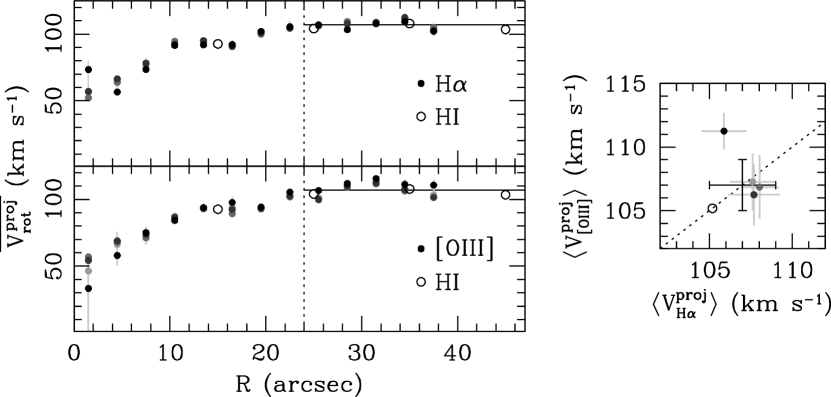
Figure 6.— The projected rotation curves for all UGC 463 gas tracers determined by four different weighting schemes (see Appendix B): from light-gray to black, the weights are uniform, error-based, from $\cos\theta$, and from $\partial V_{\rm LOS}/\partial i$. Left — The projected H$\alpha$ (filled points in the top panel), [O iii] (filled points in the bottom panel), and H i (open points) rotation curves. Measurements of $\langle V_{\rm rot}^{\rm proj}\rangle$ are made at $R>24\arcsec$, delineated by the vertical dotted line. The mean $\langle V_{\rm rot}^{\rm proj}\rangle$ for all tracers is plotted as a solid horizontal line. Right — Measured $\langle V_{\rm rot}^{\rm proj}\rangle$ for the H$\alpha$- (abcissa) and [O iii]-emitting (ordinate) gas for all four weighting schemes; the dotted lines gives the 1:1 relation between the two tracers; $\langle V_{\rm rot}^{\rm proj}\rangle$ for H i is plotted as an open circle on this relation. The black error bars show $\langle V_{\rm rot}^{\rm proj}\rangle=107\pm 2$ determined using all three gas tracers.

The calculation of $i_{\rm TF}$ and its uncertainty relies on two additional factors: (1) the choice of the TF relation and (2) the estimation of its intrinsic scatter. V01 created multiple samples based on a rotation-curve- and asymmetry-based taxonomy, each sample yielding different TF coefficients ($c_{1,\lambda}$ and $c_{2,\lambda}$) and intrinsic-scatter estimates. UGC 463 exhibits H i and ionized-gas properties that are most consistent with the “RC/$FD$” sample from V01 (see his Sections 4 and 5 for a detailed definition of this sample); UGC 463 fits within the definition of the “RC/$FD$” sample because its rotation curve asymptotes to a nearly constant rotation speed and exhibits neither strong rotation asymmetries (Section 4.2) nor signs of ongoing interaction. Additionally, V01 produced TF coefficients based on two fiducial velocities, one measured at the rotation-curve peak ($V_{\rm max}$) and the other where it “flattened” to a constant value ($V_{\rm flat}$). UGC 463 exhibits a well-defined $V_{\rm flat}$ (Figure 6); however, in most cases $V_{\rm flat}=V_{\rm max}$ for galaxies studied by V01. The smallest observed scatter in the $K$-band TF relations derived by V01 (0.26 mag) was found by excluding the outlying NGC 3992 measurements from the “RC/$FD$” sample (leaving measurements for 21 galaxies) and using $V_{\rm flat}$ for the fiducial rotation measurement; this TF relation is consistent with having zero intrinsic scatter.

Given the range in $c_{1,K}$ and $c_{2,K}$ for the “RC/$FD$” sample (with and without NGC 3992 and based on either $V_{\rm max}$ or $V_{\rm flat}$) from Table 4 of V01, we find $28\arcdeg\leq i_{\rm TF}\leq 30\arcdeg$; and we find $\epsilon(i_{\rm TF})=1\arcdeg$ and $2\arcdeg$ assuming, respectively, 0.0 and 0.2 magnitudes of intrinsic TF scatter, regardless of the assumed $c_{1,K}$ and $c_{2,K}$. Taking a mean across the four relevant TF relations and assuming 0.2 magnitudes for the intrinsic TF scatter, we measure $i_{\rm TF}=29\arcdeg\pm 2\arcdeg$ for UGC 463; this measurement of $i_{\rm TF}$ is dominated by systematic error with roughly equal contributions from the uncertainties in $H_{0}$ and the TF relation. Our conservative approach to measuring $i_{\rm TF}$ is justified given that, at $M_{K}=-24.59\pm 0.15$, UGC 463 is more luminous than any galaxy considered by V01, far away from the “pivot” point of the fitted $K$-band TF relations ($M_{K}\sim-22$).

3.2. Position Angle and Dynamical Center

The kinematic position angles derived in Section 3.1.1 are very consistent among all dynamical tracers; Table 4 provides an error-weighted mean value of $\phi_{0}=68.8\pm 0.3$, which is constant across the optical disk to good approximation (as discussed in Section 3.1.1). As stated above, the PPak data affix the dynamical center to the morphological center.

We determine the pointing of each SparsePak IFU observation relative to the dynamical center by fitting the kinematic geometry (as in Section 3.1.1) with $i$ and $\phi_{0}$ fixed. We simultaneously fit all kinematics measured from our IFS, assuming all tracers are in co-planar rotation. To do so, we apply slight offsets to $V_{\rm sys}$ according to the differences found in Table 4 such that all data can be forced to have the $V_{\rm sys}$ measured for the stars. We also allow for asymmetric drift between the gas and stars by simultaneously fitting different rotation curves to these components. Finally, we force the [O iii] and stellar kinematics determined from the SparsePak observations to have the same pointing center. During the fitting procedure, we omit velocity measurements based on the measurement error and the discrepancy with the model, as described in Appendix B, and weight according to the velocity errors, as done in Andersen & Bershady (2003).

Table 6Pointing Coordinates

	$x_{d}$	$x_{0}$	$y_{d}$	$y_{0}$
Pointing	(arcsec)	(arcsec)	(arcsec)	(arcsec)
(1)	(2)	(3)	(4)	(5)
H$\alpha$ 02Jan02 p1	0.0	$-0.1_{-0.3}^{+0.3}$	0.0	$-0.5_{-0.4}^{+0.7}$
H$\alpha$ 02Jan02 p2	0.0	$0.0_{-0.3}^{+0.3}$	0.0	$-0.2_{-0.3}^{+0.7}$
H$\alpha$ 02Jan02 p3	0.0	$0.5_{-0.2}^{+0.5}$	5.6	$6.6_{-0.4}^{+0.6}$
H$\alpha$ 02Jan02 p4	4.9	$6.6_{-0.5}^{+0.4}$	2.8	$3.3_{-0.7}^{+0.7}$
H$\alpha$ 20Oct02 p1	0.0	$0.5_{-0.3}^{+0.4}$	0.0	$0.8_{-0.9}^{+0.6}$
H$\alpha$ 20Oct02 p2	0.0	$1.3_{-0.2}^{+0.3}$	5.6	$6.7_{-0.4}^{+0.5}$
H$\alpha$ 20Oct02 p3	4.9	$5.9_{-0.2}^{+0.4}$	2.8	$4.5_{-0.6}^{+0.4}$
Mg i  23Sep06	0.0	$-1.5_{-0.3}^{+0.7}$	0.0	$-0.2_{-1.4}^{+0.8}$
Mg i  PPak	0.0	$-1.8\pm 1.0$	0.0	$1.6\pm 1.0$

Table 6 provides the resulting pointing coordinates relative to the dynamical center for each IFS observation; as with the geometric quantities in Table 4, errors are 68% confidence limits determined using bootstrap simulations. Table 6 also provides the nominal expectation for the pointings based on the dither pattern used during the observations. The kinematic fitting results are consistent with the dither pattern, if allowing for $\sim 1\arcsec$ systematic errors in the initial pointing. Moreover, reconstructed continuum images that use this pointing geometry are in good agreement with direct images from SDSS (Figure 1; Section 3.3).

3.3. Two-Dimensional Maps

Five of the nine images in Figure 1 have used an interpolation algorithm to smooth over the interstitial regions of our IFS. The continuum surface-brightness maps of our IFS (labeled $\mu_{\mbox{H$\alpha$}}$ and $\mu_{\mbox{\scriptsize Mg{$~{}\!$i}}}$) are determined via a calibration to SDSS imaging data. The detailed procedures used to both perform the surface-brightness calibration and two-dimensional interpolation are discussed in Appendix A. These interpolated kinematic maps are purely for illustration purposes, useful for qualitative assessments of our registration of the dynamical center and a discussion of the two-dimensional kinematic morphology; however, all quantitative analyses herein have been performed using the direct fiber measurements, the IFU astrometric tables, and our derived pointings.

The first column of Figure 1 demonstrates the excellent agreement among the reconstructed continuum images and the direct SDSS $g$-band image. Indeed, the central contour of both $\mu_{\mbox{H$\alpha$}}$ and $\mu_{\mbox{\scriptsize Mg{$~{}\!$i}}}$ directly overlap and are centered on the NED-provided coordinate of UGC 463. The detailed spiral structure is apparent in, particularly, the $\mu_{\mbox{\scriptsize Mg{$~{}\!$i}}}$ image due to the small PPak fibers. The isovelocity contours of the gas data appear to exhibit streaming motions associated with the spiral arm toward the south-west of the galaxy center; this is less apparent in the stellar data. Additionally, the effect of asymmetric drift is seen in the stellar velocity field as the “linearization” of the isovelocity contours toward the galaxy center, which is due to a shallower increase in the stellar rotation curve, corresponding to the steep decrease in the stellar velocity dispersion, toward larger radius. We further explore the kinematic axisymmetry in Section 4.2.

4. Azimuthally Averaged Kinematics

Analyses in Sections 5 and 6 assume UGC 463 is axially symmetric, considering only the azimuthally averaged kinematics that we derive in the following subsections. We apply beam-smearing corrections in Section 4.1 (beam-smearing corrections for the H i data are described by Martinsson, 2011) such that kinematic data from different instruments can be combined. In Section 4.2, we assess the degree of dynamical symmetry by comparing approaching- and receding-side kinematics. Finding no substantial asymmetries, we discuss the azimuthally averaged kinematics in Section 4.3.

4.1. Beam-Smearing Corrections

Our beam-smearing corrections require a characterization of the beam profile, the convolution of the point-spread function and the fiber aperture. Since no significant jitter was detected among or during the individual IFS observations, the effective fiber aperture is given by the plate-scale (yielding $2\farcs 7$ for PPak and $4\farcs 7$ for SparsePak). In Appendix A, we find that the seeing of the SDSS imaging data — $1\farcs 5$ in $g$-band and $1\farcs 2$ in $r$-band — is very close to the effective seeing of our SparsePak IFS; Martinsson (2011) provides a direct seeing measurement of $1\farcs 7$ for our PPak IFS. Our beam-smearing corrections change negligibly over the range of measured seeing; therefore, we simply adopt $1\farcs 5$ seeing to calculate all beam-smearing corrections.

Our approach to beam-smearing corrections (Paper II) depends on comparing our UGC 463 data to models of the intrinsic surface-brightness ($I$), velocity ($V$), and velocity-dispersion ($\sigma$) distributions. SDSS imaging data provide the model surface-brightness distribution; $g$-band data are used for Mg i-region IFS and $r$-band are used for H$\alpha$-region IFS. We assume a polyex parameterization to model the intrinsic rotation curve (Giovanelli & Haynes, 2002). The gas velocity dispersion is assumed to be constant with radius and isotropic. Only the H$\alpha$ data are used to describe the velocity-dispersion profile; beam-smearing corrections are marginally different if the [O iii] dispersions are used instead. For the stars, we adopt SVE axial ratios of $\alpha=\sigma_{z}/\sigma_{R}=0.6$ and $\beta=\sigma_{\theta}/\sigma_{R}$ as determined by the epicycle approximation (Section 5.2; equation 5). The model radial profile for the azimuthally averaged $\sigma_{\ast}$ ($\overline{\sigma_{\ast}}$) combines an exponential function with a cubic Legendre-polynomial perturbation at small radius; although somewhat ad hoc, this form allows for deviations from a nominal exponential while enforcing a well-behaved, exponential form at large radius. For UGC 463, deviations of $\overline{\sigma_{\ast}}$ from an exponential form are small and irrelevant to the calculated beam-smearing corrections.

Beam-smearing corrections are calculated as follows: A fit to the uncorrected data is used to generate a seed model of the intrinsic galaxy kinematics, which is then “observed” by integrating a set of Gaussian line profiles, defined by ($I,V,\sigma$), discretely sampled over the beam profile of each fiber to create a synthetic data set (Westfall, 2009). The velocity and velocity-dispersion corrections are the difference between this synthetic dataset and the model value at the center of the fiber, and they are primarily correlated with the velocity gradients across the fiber face. The beam-smearing effects are largest toward the galaxy center where the rotation curve is most steeply rising and the azimuthal coverage of each fiber is largest. The trend of the correction is to increase the measured rotation speed and decrease the measured velocity dispersion. We converge to a set of beam-smearing corrections iteratively by updating the model of the intrinsic galaxy kinematics, done by fitting the corrected observational data, and minimizing the difference between the observed and synthetic data sets.

Monte Carlo simulations demonstrate that the random errors in the beam-smearing corrections are $\lesssim 10$%; systematic errors, estimated by calculating beam-smearing corrections using SVE-shape extrema, are typically much smaller. Therefore, we adopt the quadrature sum of a 10% random error and the estimated systematic error for each fiber as the error in the beam-smearing correction; the error is always 10% for the gas data. Although lower than the upper-limit used in Paper II, this reduction in error has little effect on the error budget.

The correspondence of the uncorrected H$\alpha$, [O iii], and H i rotation curves in Figure 6, despite the factor of $\gtrsim 3$ difference in the beam size among the data sets, suggests beam-smearing corrections should be small; this expectation is in agreement with our direct beam-smearing calculations. For the ionized gas data, corrections to $V_{\rm LOS}$ are less than 2 km s^-1 for 93% of the data, with a maximum correction of 14 km s^-1. For the stellar data, $V_{\rm LOS}$ corrections are less than 2 km s^-1 for 84% and 99% of the SparsePak and PPak data, respectively; the maximum correction is 7 km s^-1 for SparsePak and 8 km s^-1 for PPak. Corrections to $\sigma_{\ast}$ are less than 5% for 91% and 99% of the SparsePak and PPak data, respectively; the maximum correction is 41% for SparsePak and 29% for PPak. Corrections to $\sigma_{\ast}$ are typically less than $\epsilon(\sigma_{\rm obs})$, with the only exceptions occurring near the galaxy center.

4.2. Axial Symmetry

Figure 7 presents individual-fiber kinematics after correcting for instrumental-broadening and beam-smearing, with point types indicating the tracer and instrument. For measurements located at in-plane azimuths within $\pm 60\arcdeg$ of the major axis, we deproject $V_{\rm LOS}$ to $V_{\rm rot}^{\rm proj}$; rotation velocities are plotted regardless of whether or not they were rejected from the velocity-field fitting discussed in Section 3. Velocity-dispersion data include all measurements made at any azimuth. We find the kinematic measurements from the different IFUs to be very well matched. Data are separated according to the approaching (negative radii) and receding sides. Figure 7 also overlays mean quantities from either side of the minor axis. We determine $\overline{V_{\rm rot}^{\rm proj}}$ for the ionized gas and stars using the velocity-field fitting procedure described in Section 3.1.1, with rejection and error-based weighting. Errors in $\overline{V_{\rm rot}^{\rm proj}}$ are 68% confidence limits calculated using bootstrap simulations. The values of $\overline{\sigma_{\rm gas}}$ and $\overline{\sigma_{\ast}}$ are error-weighted means.

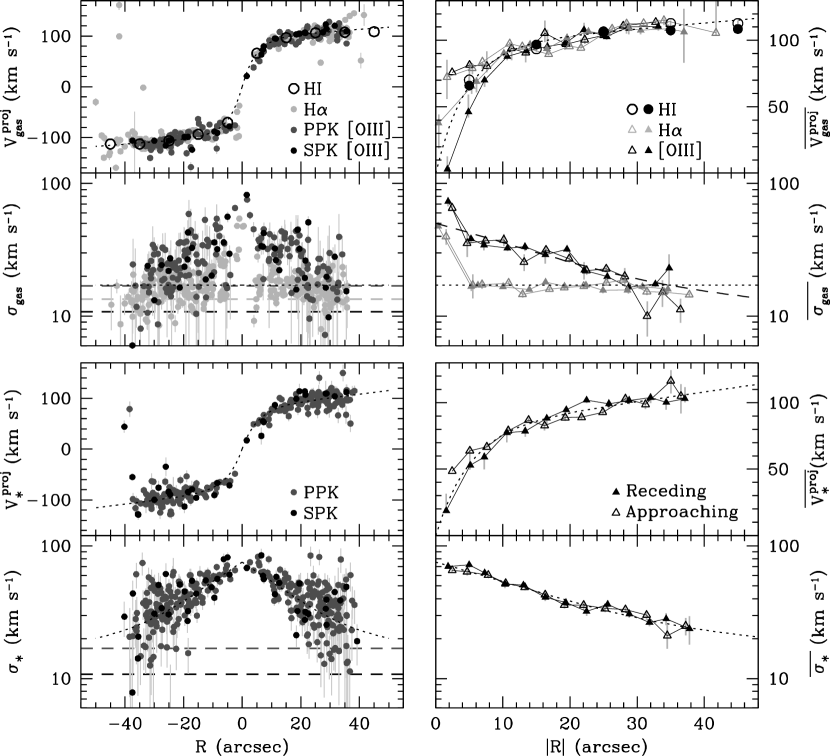
Figure 7.— Corrected gaseous ($V_{\rm gas}^{\rm proj}$, $\sigma_{\rm gas}$) and stellar ($V_{\ast}^{\rm proj}$, $\sigma_{\ast}$) kinematics for all tracers and instruments. Panels to the left present individual fiber measurements, whereas quantities in the right panels are azimuthally averaged over the approaching (open symbols) and receding (filled symbols) sides. Horizontal dashed lines mark the mean instrumental dispersion for the SparsePak H$\alpha$-region data (light gray), PPak Mg i-region data (dark gray), and SparsePak Mg i-region data (black). Model expectations used to calculate the beam-smearing corrections are shown as dotted lines. The diagonal dashed line in the $\overline{\sigma_{\rm gas}}$ panel is equal to $2/3$ of the model $\overline{\sigma_{\ast}}$ shown in the bottom-right panel.

The overlay of the binned data in Figure 7 from its two sides show that UGC 463 exhibits little kinematic asymmetry, justifying our assumption of axisymmetry in the following sections. In detail, the ionized gas rotation curves exhibit the strongest asymmetry at $R\lesssim 5\arcsec$. UGC 463 is morphologically classified as an SABc galaxy (Paper I), suggesting that this low-level asymmetry may be due to non-circular motions imposed by the presence of a weak bar. This kinematic asymmetry may also be reflected in the stellar data at marginal significance. The velocity-dispersion profiles for both the gas and stars are very symmetric at all radii, more so than the rotation velocities.

4.3. Radial Kinematic Profiles

Figure 8 provides the azimuthally averaged kinematics analyzed in Sections 5 and 6, following the same procedure as described in the previous section but over all azimuth. Stellar kinematics combine both SparsePak and PPak observations, and ionized-gas kinematics incorporate all tracers from both instruments. Rotation-velocity errors (68% confidence limits) are determined using bootstrap simulations, not by, e.g., considering the difference in rotation speed between the two sides of the rotation curve; that is, we assume the disk contains no asymmetries such that any asymmetries manifest themselves as an increased error in the measured rotation speed via bootstrap simulations. The ionized-gas rotation velocity at the largest radius is averaged with the radially overlapping H i measurement to slightly extend the radial coverage. The circular-speed curve provided in Figure 8 results from applying pressure corrections to the gas rotation curve, as described in the next section.

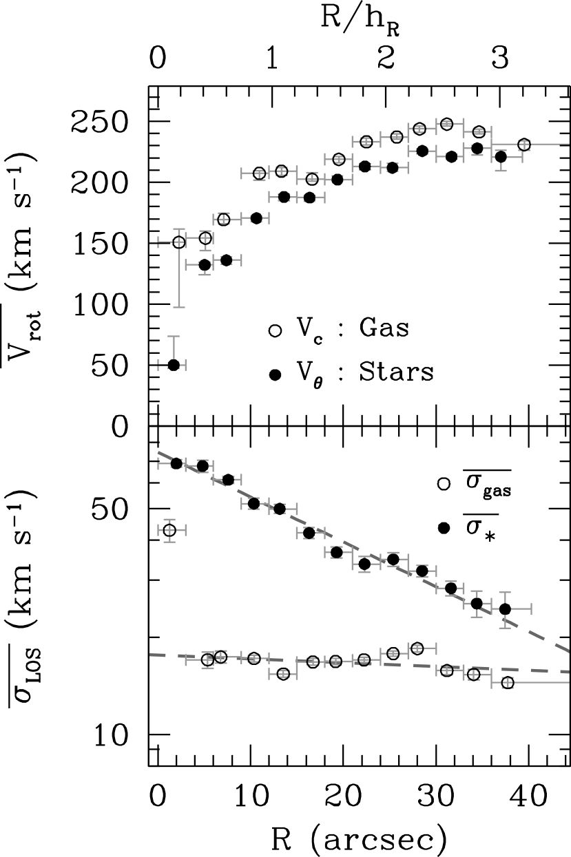
Figure 8.— Kinematic profiles for UGC 463 averaged over all azimuth. Top — Circular speed (open circles) and stellar tangential speed (filled points), as described in the text. Bottom — Gas (open circles) and stellar (filled points) LOS velocity dispersions. The dashed gray lines are the best-fitting linear and exponential functions for the gas and stellar data, respectively.

Measurements of $\overline{\sigma_{\rm gas}}$ include only the ionized-gas kinematics, not the colder H i. Although the [O iii] velocity dispersion is significantly larger than the H$\alpha$ velocity dispersion and decreasing with radius (Figure 7), the azimuthally averaged $\sigma_{\rm gas}$ is very nearly the same as the H$\alpha$ velocity dispersion. This is because of the error-weighting and the significantly higher quality of the H$\alpha$ velocity dispersions. We find $\langle\sigma_{\rm gas}\rangle=16.6\pm 1.1$ km s^-1 when excluding the datum near the galaxy center, which is nearly constant as a function of radius. This result is comparable to similar measurements made in other face-on spiral galaxies by Andersen et al. (2006) and, as shown by these authors, dominated by turbulence given the expected thermal pressure. Physically, the difference between the H$\alpha$ and [O iii] dispersions may be related to the different energetics involved in generating the two lines; for example, [O iii] emission may be naturally biased toward more turbulent regions of the ISM. From Figure 7, we note that the [O iii] dispersion is surprisingly well fit by a radial profile following $2\overline{\sigma_{\ast}}/3$ over a large radial range; it is of interest to explore the reason for this relationship by comparing with other galaxies.

4.3.1 Circular-Speed Corrections

Dalcanton & Stilp (2010) derive

$$V_{\rm c}^{2} = V_{\rm rot}^{2}-\sigma_{\rm gas}^{2}\left(\frac{d\ln\sigma_{\rm gas}^{2}}{d\ln R}+\frac{d\ln\Sigma_{\rm gas}}{d\ln R}\right)$$ (4)

$$= V_{\rm rot}^{2}+\delta_{P}\sigma_{\rm gas}^{2},$$

where $\sigma_{\rm gas}$ is assumed to be dominated by turbulence and produced by an isotropic gas velocity ellipsoid (cf. Agertz et al., 2009). We, thereby, correct our gas rotation curve to the circular speed using our measurements of the $\overline{\sigma_{\rm gas}}$ in Figure 8 and $\Sigma_{\rm gas}$ in Figure 4.

One expects $\sigma_{\rm gas}$ and $\Sigma_{\rm gas}$ to decrease with radius such that $\delta_{P}>0$. Dalcanton & Stilp (2010) propose exponential functions for use in calculating $\delta_{P}$, which is appropriate for our $\Sigma_{\rm gas}$ measurements; however, we adopt the linear function plotted in Figure 8 for $\sigma_{\rm gas}$. We calculate $0.2\leq\delta_{P}\leq 3.3$ such that the circular-speed corrections range from $0.4\leq(V_{\rm c}-V_{\rm rot})\leq 1.6$ km s^-1, always below the measurement error in the gas rotation speed. If we treat the circular-speed corrections independently for [O iii] and H$\alpha$, we find the H$\alpha$-based and [O iii]-based circular speeds to be more consistent than if one correction is applied to both. However, the combined circular-speeds are roughly independent of whether or not the H$\alpha$ and [O iii] data are treated separately.

5. The Disk

Using the data described above, we measure physical properties of the disk of UGC 463. In summary, we determine the kinematic scale length, $h_{\sigma}$, defined as the $e$-folding length of $\overline{\sigma_{\ast}}$ (Section 5.1); we determine the shape of the SVE such that we can calculate $\sigma_{z}$ based on our measurements of $\overline{\sigma_{\ast}}$ (Section 5.2); we determine the total dynamical disk mass surface density, $\Sigma_{\rm dyn}$, using equation 9 from Paper II (Section 5.3); we calculate the stellar mass surface density, $\Sigma_{\rm\ast}$, by removing contributions to $\Sigma_{\rm dyn}$ from atomic- and molecular-gas (Section 5.4); we calculate the stability of the isolated gaseous and stellar disks, as well as a quantity for the multi-component disk (Section 5.5); and, finally, we measure the dynamical and stellar mass-to-light ratios in $K$-band, $\Upsilon_{\ast,K}^{\rm disk}$ (Section 5.6).

5.1. Kinematic Scale Length, $h_{\sigma}$

Measurements of $\overline{\sigma_{\ast}}$ are well fit by an exponential profile; the best-fit exponential has a central dispersion of $74.7\pm 2.4$ km s^-1 and $h_{\sigma}=31\farcs 3\pm 1\farcs 8$ as plotted in Figure 8. Given that $h_{\sigma}\sim 2.6h_{R}$, either $\Upsilon_{\ast}$ (or more appropriately the dynamical disk mass-to-light ratio, $\Upsilon_{\rm dyn}$) or the scale height, $h_{z}$, may be increasing exponentially with radius; the implied $e$-folding length is $h_{R}h_{\sigma}/(h_{\sigma}-2h_{R})=57\farcs 5$. Over the radial range of our data, this suggests a factor of $\sim 2.3$ increase in either $\Upsilon_{\rm dyn}$ (consistent with, e.g.: Bell & de Jong, 2001; Zibetti et al., 2009) or $h_{z}$ (compare with edge-on galaxy photometry from, e.g.: van der Kruit & Searle, 1981a; de Grijs & Peletier, 1997; Narayan & Jog, 2002; Bizyaev & Mitronova, 2002; Yoachim & Dalcanton, 2006; Saha et al., 2009). The effects of radial variations in $\Upsilon_{\rm dyn}$ and/or $h_{z}$ are further discussed in Section 5.6.

5.2. Stellar Velocity Ellipsoid Axial Ratios, $\alpha$ and $\beta$

Calculations of disk mass surface density require measurements of $\sigma_{z}$. We obtain $\sigma_{z}$ by correcting $\overline{\sigma_{\ast}}$ for the shape of the SVE, which can be directly measured using stellar and ionized-gas kinematics (Shapiro et al., 2003; Noordermeer et al., 2008; Westfall, 2009). We define the two axial ratios of the SVE to be $\alpha=\sigma_{z}/\sigma_{R}$ and $\beta=\sigma_{\theta}/\sigma_{R}$. In the limit where the stellar orbits are nearly circular, the epicycle approximation (EA) yields

$$\beta^{2}=\beta_{\rm EA}^{2}\equiv\frac{1}{2}\left(\frac{\partial\ln V_{\theta}}{\partial\ln R}+1\right),$$ (5)

where $V_{\theta}$ is the tangential speed of the stars. Also, assuming that UGC 463 is axially symmetric with an SVE that is always aligned with the cylindrical coordinate axes, one can approximate

$$\delta_{\rm AD}\equiv\frac{(V_{\rm c}^{2}-V_{\theta}^{2})\sin^{2}i}{\overline{\sigma_{\ast}^{2}}}\approx\frac{\tan^{2}i}{\overline{\gamma}\alpha^{2}}\left(\frac{4R}{h_{\sigma}}+\beta^{2}-1\right)$$ (6)

from the asymmetric drift (AD) equation (Binney & Tremaine, 2008), where we use

$$\overline{\gamma}\equiv\frac{\overline{\sigma_{\ast}^{2}}}{\sigma_{z}^{2}\cos^{2}i}=1+\frac{\tan^{2}i}{2\alpha^{2}}(1+\beta^{2})$$ (7)

as defined in Paper II and $\alpha$ and $\beta$ are constant over radial regions where $\partial\ln\overline{\sigma_{\ast}^{2}}/\partial\ln R\approx-2R/h_{\sigma}$. Using these equations, each radially binned measurement of $V_{\rm c}$, $V_{\theta}$, and $\overline{\sigma_{\ast}^{2}}$ provides a direct measurement of $\beta_{\rm EA}$ and $\alpha=\alpha_{\rm AD}$, assuming that the derivatives $\partial\ln V_{\theta}/\partial\ln R$ and $\partial\ln\overline{\sigma_{\ast}^{2}}/\partial\ln R$ do not strongly deviate from the fitted-model expectations; for all measurements we assume $\overline{\sigma_{\ast}^{2}}=\overline{\sigma_{\ast}}^{2}$.

In Figure 9(a), we calculate $\beta_{\rm EA}$ for each radial ring using the parameterized description of $V_{\theta}$ shown in Figure 7. Systematic errors of greater than 15% are expected due to non-circular stellar orbits (Vandervoort, 1975; Kuijken & Tremaine, 1991; Dehnen, 1999) and non-axisymmetric streaming motions in the disk near spiral arms (Vorobyov & Theis, 2006, 2008); such effects will dominate the $\lesssim 2$% random error shown in Figure 9(a). Adopting $\beta=\beta_{\rm EA}$, Figure 9(b) provides $\alpha_{\rm AD}$ given the observed values of $\delta_{\rm AD}$ in Figure 9(c). Note that the calculation of $\alpha_{\rm AD}$ near the galaxy center provides an imaginary result ($\alpha^{2}<0$) and is not shown in Figures 9(a) or 9(b). Excluding this datum, the mean values are $\langle\alpha_{\rm AD}\rangle=0.46$ and $\langle\beta_{\rm EA}\rangle=0.81$.

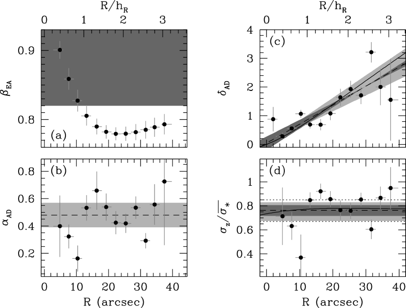
Figure 9.— SVE results for UGC 463. Dark- and light-gray regions, in any panel, show the error range in $\beta=1.04\pm 0.22$ and $\alpha=0.48\pm 0.09$, respectively, as fitted to the $\delta_{\rm AD}$ measurements in panel (c); the dashed line, in any panel, results when these axial ratios are constant at all radii. The solid line assumes $\beta=\beta_{\rm EA}$ and $\alpha=0.44\pm 0.07$ (see text). Panel (a) provides $\beta_{\rm EA}$, calculated assuming the model stellar rotation curve from Figure 7. Panel (b) provides $\alpha_{\rm AD}$ calculated assuming $\beta=\beta_{\rm EA}$ from panel (a) and measurements of $\delta_{\rm AD}$ from panel (c). Panel (d) provides measurements of $\sigma_{z}/\overline{\sigma_{\ast}}$ assuming $\alpha=\alpha_{\rm AD}$ and $\beta=\beta_{\rm EA}$. Dotted lines in panel (d) give the error range in $\sigma_{z}/\overline{\sigma_{\ast}}=0.76\pm 0.09$.

We fit equation 6 to our measurements of $\delta_{\rm AD}$ in Figure 9(c) under the assumption that the SVE shape is constant (such that $\delta_{\rm AD}$ is linear in radius). We note that $\delta_{\rm AD}$ is inversely proportional to $\alpha$, and $\delta_{\rm AD}$ pivots about $\delta_{\rm AD}=2$ — where $\delta_{\rm AD}$ is independent of $\beta$ — such that an increase in $\beta$ decreases the slope of $\delta_{\rm AD}(R)$. Errors in $\alpha$ and $\beta$ are estimated using the quadrature sum of two quantities: (1) the standard deviation returned by a Monte Carlo sampling of the normal distributions $i=27\arcdeg\pm 2\arcdeg$ and $h_{\sigma}=31\farcs 3\pm 1\farcs 8$; and (2) the mean of the error determined from a set of 500 bootstrap simulations performed for each instance of $i$ and $h_{\sigma}$. We find $\alpha=0.48\pm 0.09$ and $\beta=1.04\pm 0.22$, shown as the dashed line in Figure 9; errors are shown as light- and dark-gray regions for $\alpha$ and $\beta$, respectively. If we force $\beta=\beta_{\rm EA}$ when fitting $\delta_{\rm AD}$, we find $\alpha=0.44\pm 0.07$ with a fit shown by the solid line in Figure 9.

Figure 9(a) shows that $\langle\beta_{\rm EA}\rangle=0.81$ and $\beta=1.04\pm 0.22$ are different at the level of slightly more than the random errors. Although interesting, the relevance of this difference to our subsequent analysis is primarily with respect to our conversion of $\overline{\sigma_{\ast}}$ to $\sigma_{R}$ (see Section 5.5) and $\sigma_{z}$. Figure 9(d) provides individual measurements of the ratio $\sigma_{z}/\overline{\sigma_{\ast}}=(\overline{\gamma}\cos^{2}i)^{-1/2}$ using $\alpha_{\rm AD}$ and $\beta_{\rm EA}$. Adopting $i=27\arcdeg\pm 2\arcdeg$, $\alpha=0.48\pm 0.09$, and $\beta=1.04\pm 0.22$, we calculate the constant value $\sigma_{z}/\overline{\sigma_{\ast}}=0.76\pm 0.09$, which is identical to $\langle\sigma_{z}/\overline{\sigma_{\ast}}\rangle$ calculated using the individual measurements based on $\alpha_{\rm AD}$ and $\beta_{\rm EA}$ when excluding the datum near the galaxy center. Assuming $\alpha=0.44\pm 0.07$ and $\beta=\beta_{\rm EA}$ is insignificantly different from $\sigma_{z}/\overline{\sigma_{\ast}}=0.76\pm 0.09$, as shown by the solid line in Figure 9(d). Moreover, fitting the azimuthal variation in $\sigma_{\ast}/\overline{\sigma_{\ast}}$ averaged over the full radial range, akin to the analysis done by Gerssen et al. (1997, 2000) and Shapiro et al. (2003), provides $\beta\sim 0.9$, consistent with the error in our measurement based on $\delta_{\rm AD}$ and, therefore, insignificant to the calculation of $\sigma_{z}/\overline{\sigma_{\ast}}$.

5.3. Dynamical Disk-Mass Surface Density, $\Sigma_{\rm dyn}$

We calculate $\Sigma_{\rm dyn}$ using equation 9 from Paper II, which is fundamentally $\Sigma_{\rm dyn}=\sigma_{z}^{2}/\pi kGh_{z}$. We calculate $\sigma_{z}$ using $\overline{\sigma_{\ast}}$ and our SVE measurements above; the oblateness ratio $q=h_{R}/h_{z}$, given by equation 1 in Paper II, provides the vertical scale height, $h_{z}$, at the distance $D$; and the effect of the assumed vertical mass distribution is quantified by $k$. van der Kruit (1988) calculate the value of $k$ for three vertical mass distributions: exponential ($k=1.5$), sech ($k=1.71$), and sech² ($k=2$). As discussed in Paper II, our nominal approach is to adopt a purely exponential disk as a reasonable approximation for the composite (gas$+$stars) density distribution; thus, of the three density distributions discussed by van der Kruit (1988), we are effectively maximizing the measurement of $\Sigma_{\rm dyn}$ and, hence, $\Upsilon_{\ast,K}^{\rm disk}$. In Paper II, we suggested a 14% systematic error in $k$ based on the range in $k$ among the exponential, sech, and sech² distributions. For the case of UGC 463, we increase this to $k=1.5\pm 0.3$, allowing for a relatively massive gas disk (low $k$) or spherical DM halo (high $k$); see further discussion in Sections 5.6.1 and 6.

We use the scale length fitted to $\mu^{\prime}_{K}$ to calculate $q$ and $h_{z}$ as provided in Table 2; the band used to define $h_{R}$ is insignificant to the result. Figure 10 plots the resulting $\Sigma_{\rm dyn}$ calculations along with the measurements of $\Sigma_{\mbox{\rm\footnotesize H{i}}}$ and $\Sigma_{\rm H_{2}}$ from Sections 2.5 and Section 2.6.3, respectively. Random (including contributions from $V_{\rm sys}$, $m_{K}$, $i$, $h_{R}$, $\overline{\sigma_{\ast}}$, $\alpha$, and $\beta$) and systematic (including contributions from $q$, $k$, and $D$) errors are calculated separately; the former are dominated by the error in the SVE and the latter have roughly equal contributions from $k$ and $q$ ($\sim 20-25$%). For clarity, Figure 10 shows neither the systematic error in $\Sigma_{\rm dyn}$ nor any errors in $\Sigma_{\mbox{\rm\footnotesize H{i}}}$ and $\Sigma_{\rm H_{2}}$; the systematic errors in $\Sigma_{\rm dyn}$ are comparable to the random errors. Computing the total gas mass surface density, we find a very reasonable fit to $\Sigma_{\rm dyn}$ by scaling $\Sigma_{\rm gas}$ by a factor of 3, akin to the correlation of $\Sigma_{\rm gas}$ with $\mu^{\prime}_{K}$ shown in Figure 4; $\Sigma_{\mbox{\rm\footnotesize H{i}}}$ and $\Sigma_{\rm H_{2}}$ have been interpolated to the radii of the $\overline{\sigma_{\ast}}$ measurements for this comparison.

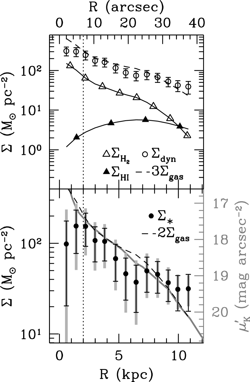
Figure 10.— Mass surface density measurements for UGC 463. The total dynamical ($\Sigma_{\rm dyn}$; open circles), H i ($\Sigma_{\mbox{\rm\footnotesize H{i}}}$; filled triangles), H₂ ($\Sigma_{\rm H_{2}}$; open triangles), and stellar ($\Sigma_{\rm\ast}$; filled circles) mass surface densities are plotted as a function of radius. Random errors (black error bars) are plotted for both $\Sigma_{\rm dyn}$ and $\Sigma_{\rm\ast}$; systematic errors (light-gray error bars) are plotted only for $\Sigma_{\rm\ast}$. As described in the text, dashed lines provide $3\Sigma_{\rm gas}$ and $2\Sigma_{\rm gas}$ in the top and bottom panels, respectively. The vertical dotted line marks the radius beyond which the Sérsic profile describing the intrinsic central light concentration (Section 2.2.2) contributes less than 3% to $\mu^{\prime}_{K}$. We overplot $\mu^{\prime}_{K}$ (thick gray line) in the bottom panel with a scaling such that $\Sigma_{\rm\ast}$ data falling directly on the surface-brightness measurements have $\Upsilon_{\ast,K}^{\rm disk}\sim 0.2$.

5.4. Stellar Disk-Mass Surface Density, $\Sigma_{\rm\ast}$

Calculations of $\Upsilon_{\ast,K}^{\rm disk}$ require a decomposition of $\Sigma_{\rm dyn}$ into stellar and non-stellar components. Five mass components contribute to $\Sigma_{\rm dyn}$: stars, atomic gas, molecular gas, dust, and other non-stellar matter. However, we account for only the first three listed; the others are subsumed in the “stellar” mass surface density, $\Sigma_{\rm\ast}$, for the following reasons. First, our data do not provide dynamically differentiable measurements of the stellar-remnant and other DM (baryonic or otherwise) mass. Second, the total dust mass of normal star-forming (or even star-bursting) spiral galaxies is expected to be less than 10% (and more typically $\sim 1$%) of the total hydrogen mass (Draine et al., 2007); therefore, it should not be dynamically important to the mass surface density at scales relevant to our analysis.

Our measurements of $\Sigma_{\rm\ast}=\Sigma_{\rm dyn}-1.4(\Sigma_{\mbox{\rm\footnotesize H{i}}}+\Sigma_{\rm H_{2}})$ are presented in the bottom panel of Figure 10. As with $\Sigma_{\rm dyn}$, we calculate random and systematic errors in $\Sigma_{\rm\ast}$ separately; compared with $\Sigma_{\rm dyn}$, $\Sigma_{\rm\ast}$ includes additional random error from $I_{24\mu{\rm m}}$ and $\Sigma_{\mbox{\rm\footnotesize H{i}}}$ and systematic error from the $I_{24\mu{\rm m}}/I_{\rm CO}\Delta V$ calibration and $X_{\rm CO}$. Given the modest errors in $I_{24\mu{\rm m}}$ and $\Sigma_{\mbox{\rm\footnotesize H{i}}}$, the random error in $\Sigma_{\rm\ast}$ is dominated by the errors in $\sigma_{z}$; and, despite the large systematic uncertainties in $I_{24\mu{\rm m}}/I_{\rm CO}\Delta V$ and $X_{\rm CO}$ (roughly 30% for both), the systematic errors in $\Sigma_{\rm\ast}$ are dominated by the errors in $k$ and $q$. We plot our $\Sigma_{\rm\ast}$ measurements against $2\Sigma_{\rm gas}$ and $\mu^{\prime}_{K}$ (Section 2.2.2); the scale of the plot is such that all $\Sigma_{\rm\ast}$ measurements falling on the $\mu^{\prime}_{K}$ profile have $\Upsilon_{\ast,K}^{\rm disk}\sim 0.2$. We find that $\Sigma_{\rm\ast}(R)$ is roughly consistent with both $2\Sigma_{\rm gas}$ and $\mu^{\prime}_{K}$ at the level of the random errors.

5.5. Global Stability, $Q$

We calculate the global stability, $Q$, of the gaseous and stellar disks separately and for the composite disk using our mass-surface-density and velocity-dispersion measurements. These calculations are of interest to our dynamical study of UGC 463 given our measurement of a systematically low $\Sigma_{\rm dyn}$ with respect to a maximal disk (see Section 6): A dependence between spiral-arm multiplicity and disk maximality is expected (Toomre, 1981; Athanassoula et al., 1987) based on stability arguments within the context of swing-amplification theory — see reviews by Athanassoula (1984) and Sellwood (2010). Qualitatively, one expects a higher spiral-arm multiplicity for lower surface density disks of a fixed rotation curve. This expectation is in line with our measurement of a submaximal disk for and the three-arm multiplicity of UGC 463 (see Figure 1); however, it should be noted that we find submaximal disks for all 30 galaxies we have studied so far (Paper V; Martinsson, 2011), regardless of their spiral structure. Stability issues will be discussed at greater length based on our full survey stemming from the simple analysis given as an example here for UGC 463.

Assuming a razor-thin disk, Toomre (1964) derived

$$Q_{\rm T,gas} = \frac{\kappa\ c_{s}}{\pi\ G\ \Sigma_{\rm gas}}$$ (8)

$$Q_{{\rm T,}\ast} = \frac{\kappa\ \sigma_{R}}{3.36\ G\ \Sigma_{\rm\ast}},$$ (9)

where

$$\kappa^{2}=2\frac{V_{\rm c}}{R}\left(\frac{V_{\rm c}}{R}+\frac{dV_{\rm c}}{dR}\right)$$ (10)

is the epicyclic frequency and $c_{s}$ is the sound speed in the gas; such disks should be stable if $Q_{\rm T}>1$. Following Jog & Solomon (1984) by treating both the gaseous and stellar disks as fluids, Rafikov (2001) derived a combined stability criterion

$$\frac{1}{Q_{\rm R}}=\frac{2}{Q_{{\rm R,}\ast}}\ \frac{\omega}{1+\omega^{2}}+\frac{2}{Q_{\rm R,gas}}\ \frac{r\omega}{1+r^{2}\omega^{2}},$$ (11)

where $Q_{{\rm R,}\ast}/Q_{{\rm T,}\ast}=3.36/\pi$, $Q_{\rm R,gas}=Q_{\rm T,gas}$, $\omega=k_{\lambda}\sigma_{R}/\kappa$, $k_{\lambda}=2\pi/\lambda$ is the wavenumber of the instability, and $r=c_{s}/\sigma_{R}$; this multi-component, razor-thin disk is stable if $Q_{\rm R}>1$. The finite thickness of disks systematically increases the stability over that estimated via the equations above; however, finite-thickness corrections are small (Romeo, 1992).

Figure 11 provides our measurements of $Q$ for the disk of UGC 463; all measurements demonstrate global stability. To calculate $\kappa$, we use the derivative of equation 4 to calculate $dV_{\rm c}/dR$, adopting the model gas rotation curve from Figure 7 and the model $\sigma_{\rm gas}$ and $\delta_{P}$ functions discussed in Section 4.3.

Given that turbulence dominates the gas kinematics (Section 4.3), we calculate $Q_{\rm T,gas}$ by replacing $c_{s}$ with our measurements of $\overline{\sigma_{\rm gas}}$ from the ionized gas. Therefore, our measurements of $Q_{\rm T,gas}$ may represent upper limits; the measured $\langle\sigma_{\rm gas}\rangle=16.6\pm 1.1$ km s^-1 for UGC 463 is a factor of two or more greater than the typical turbulent motions seen in the H i or H₂ gas observed in local spiral galaxies (Hitschfeld et al., 2009; Tamburro et al., 2009). Figure 11 shows that $Q_{\rm T,gas}$ increases monotonically for $R\gtrsim 4$ kpc. In the range 2 kpc $\lesssim R\lesssim 7$ kpc ($0.6\lesssim R/h_{R}\lesssim 2.0$), we find $\langle Q_{\rm T,gas}\rangle=1.83\pm 0.04^{+0.79}_{-0.72}$. Thus, in the absence of the stellar disk, the gas disk would be globally stable, but only by $\sim 1.2$ times the error. A factor of two decrease in $\overline{\sigma_{\rm gas}}$ would produce an unstable gas disk, when in the absence of the stellar component.

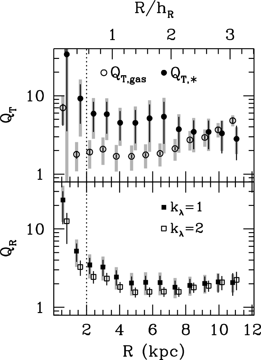
Figure 11.— Disk stability measurements for the isolated gaseous (open circles) and stellar (filled points) disks following from equations derived by Toomre (1964, $Q_{\rm T}$, top) are plotted in the top panel. The multi-component disk stability from Rafikov (2001, $Q_{\rm R}$, bottom) for wavenumbers of $k_{\lambda}=1$ (black squares) and $k_{\lambda}=2$ (gray squares) are provided in the bottom panel. Values of $Q_{\rm T,gas}$ and $Q_{{\rm T,}\ast}$, and $Q_{\rm R}$ for different $k_{\lambda}$, are slightly offset in radius for clarity. Random errors are plotted in black; systematic errors, not provided for $Q_{\rm R}$ when $k_{\lambda}=2$, are plotted in light gray. The vertical dotted line is the same as plotted in Figure 10.

The calculation of $Q_{{\rm T,}\ast}$ is determined directly from the data shown in Figures 8 and 10, where we calculate $\sigma_{R}=(1.59\pm 0.17)\overline{\sigma_{\ast}}$ using our measurements of the SVE axial ratios (Section 5.2). We find $\langle Q_{{\rm T,}\ast}\rangle=5.2\pm 2.1^{+3.1}_{-2.2}$ between 2 kpc $\lesssim R\lesssim 7$ kpc, decreasing to $\sim 0.6Q_{\rm T,gas}$ at the radial limit of our data. The isolated stellar disk appears to be extremely stable, in stark contrast to nominal expectations ($Q\sim 2$) based on empirical (e.g., Bottema, 1993) or theoretical (e.g., Sellwood & Carlberg, 1984) arguments. Given the mass of the gaseous disk, a measurement of the composite stability is physically more meaningful.

The multi-component-disk stability measurement $Q_{\rm R}$ asymptotically decreases to $Q_{\rm R}\sim 2$, more in line with the theoretical expectations. In detail, we find $\langle Q_{\rm R}\rangle=2.1\pm 0.4\pm 0.7$ at $R\gtrsim h_{R}$ for $k_{\lambda}=1$ indicating a globally stable disk; measurements assuming $k_{\lambda}=2$, also provided in Figure 11, reduce $Q_{\rm R}$ by no more than its error. A factor of two reduction in $\overline{\sigma_{\rm gas}}$ decreases $\langle Q_{\rm R}\rangle$ at $R\gtrsim h_{R}$ by 4% and 20% for $k_{\lambda}=1$ and 2, respectively, such that the composite disk should remain stable in this limit.

5.6. $K$-Band Mass-to-Light Ratios, $\Upsilon_{{\rm dyn},K}^{\rm disk}$ and $\Upsilon_{\ast,K}^{\rm disk}$

We calculate dynamical ($\Upsilon_{{\rm dyn},K}^{\rm disk}$) and stellar ($\Upsilon_{\ast,K}^{\rm disk}$) mass-to-light ratios using our measurements of $\Sigma_{\rm dyn}$ and $\Sigma_{\rm\ast}$, respectively, and the $K$-band surface-brightness

$$I^{\rm disk}_{K} = {\rm dexp}[-0.4(\mu^{\prime}_{K}-A^{i}_{K}-{\mathcal{K}}-M_{\odot}^{K}-21.57)]\times$$ (12)

$$\left(1-\frac{I_{K}^{\rm dust}}{I_{K}^{\rm obs}}\right)\cos i$$

in $\mathcal{L}_{\odot}^{K}{\rm pc}^{-2}$, where $I_{K}^{\rm obs}$ is the observed emission after correcting for Galactic extinction, $A^{i}_{K}$ is the internal dust extinction in magnitudes (Section 2.2.4), ${\mathcal{K}}=0.035$ mag is the ${\mathcal{K}}$-correction (Bershady, 1995), $I_{K}^{\rm dust}/I_{K}^{\rm obs}=0.02\pm 0.01$ is the fraction of dust emission in the $K$-band (Section 2.2.5), $i=27\arcdeg\pm 2\arcdeg$ is the inclination (Section 3.1), and $M_{\odot,K}=3.30\pm 0.04$ is the absolute magnitude of the Sun. Equation 10 from Paper II did not include some terms in equation 12, the most significant of which ($0.125\pm 0.019$ mag arcsec^-2) is the face-on correction ($\cos i$); such terms negligibly affect our error budget.

Figure 12 provides our measurements of $\Upsilon_{{\rm dyn},K}^{\rm disk}=\Sigma_{\rm dyn}/I_{K}^{\rm disk}$ and $\Upsilon_{\ast,K}^{\rm disk}=\Sigma_{\rm\ast}/I_{K}^{\rm disk}$, both in units of $\mathcal{M}_{\odot}/\mathcal{L}_{\odot}^{K}$; the difference illustrates the effect of the gas-mass correction. These data are plotted both as a function of radius and $(g-i)_{0}$ color. Given our dynamical assumptions (e.g., negligible radial forces), $\Sigma_{\rm dyn}$ measurements at small radius may be systematically in error, especially in the presence of a pressure-dominated bulge (as possible given the central light concentration; Section 2.2.2), a weak bar (Section 4.2), or a massive halo (Section 6). The vertical dashed lined in Figure 12 marks where our model of the central light concentration contributes less than 3% to the total light; $\Sigma_{\rm dyn}$ measurements beyond this radius (i.e., $R\geq 2$ kpc) should not be strongly affected by either the “bulge” or the dynamical assumptions. The two measurements of $\Upsilon_{{\rm dyn},K}^{\rm disk}$ and $\Upsilon_{\ast,K}^{\rm disk}$ within this radius are not plotted as a function of $(g-i)_{0}$. Measurements of $(g-i)_{0}$ are interpolated from our SDSS photometry (Section 2.2.1) after accounting for internal reddening (Section 2.2.4); instrumental-smoothing- and ${\mathcal{K}}$-corrections have not been applied to the $g$- or $i$-band data. We compare our dynamical measurements with SPS model calculations in Figure 12 by plotting

$$\Upsilon_{\ast,K}^{\rm SPS}={\rm dexp}[a_{K}+b_{K}(g-i)_{0}],$$ (13)

where the coefficients $a_{K}$ and $b_{K}$ are taken from Bell et al. (2003, $a_{K}=-0.211$ and $b_{K}=0.137$, hereafter B03) and Zibetti et al. (2009, $a_{K}=-1.379$ and $b_{K}=0.604$, hereafter Z09); these models roughly represent the extrema of similar SPS modeling done by, e.g., Bell & de Jong (2001) and Portinari et al. (2004). Consistent with our photometry in Section 2.2, B03 and Z09 assume $K$-band measurements are in Vega magnitudes and $g$- and $i$-band measurements are in AB magnitudes. We discuss our results below after generating approximate probability distributions for $\Upsilon_{\ast,K}^{\rm disk}(R)$ and $\langle\Upsilon_{\ast,K}^{\rm disk}\rangle$.

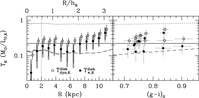
Figure 12.— Measurements of $\Upsilon_{\ast,K}^{\rm disk}$ (filled points) and $\Upsilon_{{\rm dyn},K}^{\rm disk}$ (open circles) as a function of radius (left) and $(g-i)_{0}$ color (right); the $\Upsilon_{{\rm dyn},K}^{\rm disk}$ measurements are slightly offset in radius from the $\Upsilon_{\ast,K}^{\rm disk}$ measurements for clarity. Random errors are plotted in black; systematic errors, only plotted for $\Upsilon_{\ast,K}^{\rm disk}$ in the left panel, are light gray. The vertical dotted line delineates the radius at which the central light concentration contributes $\sim 3$% to the total flux ($R=2$ kpc); data within this radius are not shown in the right panel. The solid dark-gray line provides the mean $\Upsilon_{\ast,K}^{\rm disk}$ at $R>2$ kpc. The $(g-i)_{0}$ colors are used to predict $\Upsilon_{\ast,K}^{\rm SPS}$ based on the work of B03 (dotted line) and Z09 (dashed line); random errors due to the photometry are shown by the surrounding gray regions in the left panel.

5.6.1 Probability Distribution

We create an approximate probability distribution (combining random and systematic components) for our measurements of $\Upsilon_{\ast,K}^{\rm disk}(R)$ and $\langle\Upsilon_{\ast,K}^{\rm disk}\rangle$ by Monte Carlo (MC) sampling individual probability distributions for each component of our $\Upsilon_{\ast,K}^{\rm disk}$ calculation. In contrast to the random error contributors, systematic errors — particularly in $q$, $k$, and $X_{\rm CO}$ — may not be normally distributed, providing the primary motivation for this test. Our simulation is limited by the exclusion of any parameter covariance, such as might be manifest in a refitting of $\alpha$ and $\beta$ after adjusting $i$; however, we do not expect parameter covariance to dramatically change the fundamental conclusions drawn from this MC simulation.

Random-error contributors — all quantities with measurement errors contributing to the random error in $\Upsilon_{\ast,K}^{\rm disk}$ — are assigned Gaussian probability distributions according to their derived $\epsilon$. We also assign a Gaussian distribution for $D$ (combining the random and systematic error in quadrature) and $I_{24\mu{\rm m}}/I_{\rm CO}\Delta V$ (using the $\pm 0.11$ dex error in equation 1). Information on the probability distribution for $X_{\rm CO}$, particularly for spiral galaxies like UGC 463, is limited; therefore, we simply assume a uniform distribution with the range $X_{\rm CO}=(2.7\pm 0.9)\times 10^{20}$ cm^-2 (K km s^-1)^-1 (Section 2.6.3). We have derived an empirical probability distribution for $q$ in Paper II (see Figure 1, and references, therein). For our MC simulation, we smooth the growth curve of this empirical distribution by a low-order polynomial to avoid the discrete-measurement quantization noise.

A robust probability distribution for $k$ is elusive, lacking an empirical measurement. For UGC 463, the measurements of a relatively massive gas disk (Section 2.7) and DM halo (Section 6) are particularly relevant to the value of $k$. In an extreme scenario, the stellar disk is vertically exponential and the gas disk is razor thin, yielding an effective 30% decrease in $k$ for our measured values of $\Sigma_{\rm gas}$ and $\Sigma_{\rm\ast}$. Despite the resulting increase in $\Sigma_{\rm dyn}$, we would still infer a massive DM halo that increases $k$ by $20-30$% (Section 6.3.2) and, therefore, roughly offsets the effect of the massive gas disk. In view of further complications introduced by finite-thickness gas disks, multi-component stellar disks, and triaxial halos, we have decided to take a simple approach and assume $k$ is quantized and equally distributed among the exponential ($k=1.5$), sech ($k=1.71$), and sech² ($k=2.0$) cases.

The results of our MC simulation are shown in Figure 13 based on $10^{6}$ recalculations of $\Upsilon_{\ast,K}^{\rm disk}$ for each measurement of $\overline{\sigma_{\ast}}$ at $R\geq 2$ kpc. Each recalculation is binned in the two-dimensional ($R$, $\Upsilon_{\ast,K}^{\rm disk}$) plane; $R$ is binned in physical units, incorporating the MC sampling of $D$. For each radial bin, we create a growth curve for $\Upsilon_{\ast,K}^{\rm disk}$ such that higher intensity (darker) cells in the left panel of Figure 13 represent more probable measurement of $\Upsilon_{\ast,K}^{\rm disk}$. We overplot 68%, 95%, and 99% confidence contours for $\Upsilon_{\ast,K}^{\rm disk}(R)$, as well as a contour following the median value. We also overplot the nominal measurements of $\Upsilon_{\ast,K}^{\rm disk}$ from Figure 12 for reference, again differentiating between random and systematic error. Figure 13 also provides the growth curve of $\langle\Upsilon_{\ast,K}^{\rm disk}\rangle$, calculated for each of the $10^{6}$ recalculations of $\Upsilon_{\ast,K}^{\rm disk}(R)$.

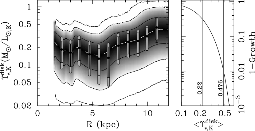
Figure 13.— Result of the Monte Carlo simulation outlined in Section 5.6.1. The left panel shows the gray-scale image of the folded growth curve in $\Upsilon_{\ast,K}^{\rm disk}$ at a given radius. The median $\Upsilon_{\ast,K}^{\rm disk}(R)$ lies at the peak intensity (black) as traced by the dashed white line; black contours mark the 68%, 95%, and 99% confidence intervals. The nominal measurements of $\Upsilon_{\ast,K}^{\rm disk}(R)$ from Figure 12 are overplotted (black points) with random and systematic errors in black and gray, respectively; data at $R<2$ kpc are omitted. The growth curve of $\langle\Upsilon_{\ast,K}^{\rm disk}\rangle$ is plotted in the right panel. Gray lines mark $\langle\Upsilon_{\ast,K}^{\rm disk}\rangle=0.22$ and 0.476; less than 1% and 0.1% of the simulations produce $\langle\Upsilon_{\ast,K}^{\rm disk}\rangle>0.476$ and $\langle\Upsilon_{\ast,K}^{\rm disk}\rangle>0.59$, respectively.

5.6.2 Discussion

Based on our nominal calculation (Figure 12), we find $\langle\Upsilon_{{\rm dyn},K}^{\rm disk}\rangle=0.34\pm 0.09\pm 0.15$ and $\langle\Upsilon_{\ast,K}^{\rm disk}\rangle=0.22\pm 0.09^{+0.16}_{-0.15}$ at $R>2$ kpc, in units of $\mathcal{M}_{\odot}/\mathcal{L}_{\odot}^{K}$. In contrast, B03 and Z09 predict $\langle\Upsilon_{\ast,K}^{\rm SPS}\rangle=3.6\langle\Upsilon_{\ast,K}^{\rm disk}\rangle$ and $\langle\Upsilon_{\ast,K}^{\rm SPS}\rangle=0.56\langle\Upsilon_{\ast,K}^{\rm disk}\rangle$, respectively. From our derived probability distribution we find a median of $\langle\Upsilon_{\ast,K}^{\rm disk}\rangle=0.17^{+0.12}_{-0.09}$ such that the Z09 prediction is within our 68% confidence interval; however, B03 predict a measurement that occurs for less than 1 in $10^{5}$ recalculations of $\langle\Upsilon_{\ast,K}^{\rm disk}\rangle$. The median value of our probability distribution is below our nominal measurement because the median value for $k$ is above our nominal value of $k=1.5$. Within the parameter space probed by our MC simulation, we find a maximum measurement of $\langle\Upsilon_{\ast,K}^{\rm disk}\rangle=0.82$.

The prescriptions adopted for the many ingredients of SPS modeling — such as the initial mass function (IMF), star-formation and chemical-enrichment history, dust content, and the treatment of specific phases of stellar evolution — play an important role in setting $\Upsilon_{\ast,K}^{\rm SPS}$ and its trend with color (Portinari et al., 2004; Conroy et al., 2009, 2010; Conroy & Gunn, 2010). Indeed, in their discussion of the differences between their $\Upsilon_{\ast}$–color relations and those from B03, Z09 isolate their treatment of the star-formation histories and thermally pulsating asymptotic giant branch (TP-AGB) phases of stellar evolution from intermediate-age populations as the primary culprits. The latter particularly effects differences in SPS predictions of $\Upsilon_{\ast}$ in the NIR bands (Maraston, 2005). Aside from the factor of $\sim 7$ difference in the mean B03 and Z09 predictions for UGC 463, it is also important to keep in mind that there is an additional factor of 2 or more internal variation in the $\Upsilon_{\ast,K}^{\rm SPS}$ calibration associated with each study as determined by their search of the SPS modeling parameter space. It is encouraging that the advancement in SPS modeling, as represented by the Z09 study, are more consistent with our dynamical measurements. However, Figure 12 shows that neither the zeropoint nor the trend of $\Upsilon_{\ast}$ with $(g-i)$ color from these models are a good match to our measurements; therefore, we cannot conclude that this specific SPS treatment — either for the TP-AGB phase or star-formation histories — is correct or applicable to our entire sample. An absolute calibration of $\Upsilon_{\ast}$ using a multi-color approach for the full DMS Phase-B sample will be presented in forthcoming papers.

As expected from the discussion in Section 5.1, Figure 12 shows $\Upsilon_{{\rm dyn},K}^{\rm disk}$ and $\Upsilon_{\ast,K}^{\rm disk}$ generally increase with radius. Considering only the data at $R=5.6$ and 10.8 kpc, $\Upsilon_{{\rm dyn},K}^{\rm disk}$ and $\Upsilon_{\ast,K}^{\rm disk}$ increase by a factor of $2.2\pm 1.0^{+1.2}_{-1.1}$ and $3.4\pm 2.3^{+2.8}_{-2.5}$, respectively. Figure 13 shows that the radial trend holds for the median of the probability distribution in $\Upsilon_{\ast,K}^{\rm disk}(R)$. Variation in $\Upsilon_{\ast,K}^{\rm SPS}$ is expected in galaxy disks given the observed arm/inter-arm and radially averaged color gradients. Yet, in terms of the latter, Figure 12 shows that the variation in $\Upsilon_{\ast,K}^{\rm disk}$ for UGC 463 is consistent with neither of the plotted $\Upsilon_{\ast,K}^{\rm SPS}$ predictions. Given both the errors in our measurement and the errors in the $\Upsilon_{\ast,K}^{\rm SPS}$ calibration, it is difficult for us to conclude that our measurements are inconsistent with a radially invariant $\Upsilon_{\ast,K}^{\rm disk}$. Indeed, a radially independent $\Upsilon_{\ast,K}^{\rm disk}$ is consistent with our 68% confidence limits derived in Figure 13.

Moreover, the more shallow decline of $\sigma_{z}^{2}$ with respect to the surface-brightness profile, which is the primary driver for our measurement of a radially varying $\Upsilon_{\ast,K}^{\rm disk}$, may also be interpreted as a flaring of the stellar disk (Section 5.1). A flared stellar disk has been measured for the Galaxy (López-Corredoira et al., 2002; Robin et al., 2003; Momany et al., 2006) and one might expect disks to be flared due to, e.g., interactions with dark and/or luminous satellites (Hayashi & Chiba, 2006; Dubinski et al., 2008; Read et al., 2008; Kazantzidis et al., 2009). Indeed, Herrmann et al. (2009) suggest their measurements of a nearly constant $\sigma_{z}$ at large radii in M 83 and M 94 provide evidence for such interactions. However, the onset radius for disk flaring is expected to be beyond the region relevant to our dynamical measurements for UGC 463. Robust photometric evidence for stellar-disk flares in edge-on galaxies remains elusive: The empirical and theoretical foundation for the vertical structure of galaxy disks with radially independent scale heights developed by van der Kruit & Searle (1981a, b, 1982a, 1982b) remains the current paradigm due to repeated confirmations of little to no variation in scale height measurements from surface photometry, particularly for galaxies of similar Hubble type to UGC 463 (SABc) (e.g., de Grijs & Peletier, 1997; Bizyaev & Mitronova, 2002). However, claims of factors of 2 or more increase in scale height within the optical extent of some stellar disks exist in the literature (e.g., Narayan & Jog, 2002; Saha et al., 2009). For our UGC 463 data, the measured increase in $\Upsilon_{\ast,K}^{\rm disk}$ with radius is consistent with these claims; however, we cannot claim a stellar-disk flare exists in UGC 463 based solely on our data. Therefore, barring more detailed information on the disk structure of UGC 463, we simplify our mass decomposition in Section 6 by largely focusing on results that assume $\Upsilon_{\ast,K}^{\rm disk}$ and $h_{z}$ are constant for the entire disk.

Finally, we note that our data provide a few, limited assessments of the presence of a “DM disk” in UGC 463. Such a structure has been predicted by recent simulations (e.g., Read et al., 2009) and modeling of the Galaxy by Kalberla (2003) (cf., Moni Bidin et al., 2010). DM disks are expected to be more extended both radially and vertically than stellar thin disks; Kalberla (2003) fit a DM disk that has a scale length and scale height that are, respectively, three and 10 times larger than for the stellar thin disk. Our stellar kinematic data are expected to trace the thin disk mass distribution only such that we can place an upper limit on any DM distributed identically to this structure as follows: Assuming the $\Upsilon_{\ast,K}^{\rm SPS}$ prediction from Z09 is exactly correct, our $\Upsilon_{\ast,K}^{\rm disk}$ measurements suggest a thin DM disk that has $\sim 80$% of the stellar mass surface density (or $\sim 30$% of the baryonic mass surface density). One can increase the mass surface density of a DM disk in UGC 463 by proportionally increasing its scale height with relatively moderate effects on our calculation of $\Sigma_{\rm dyn}$. Assuming no influence on $\Sigma_{\rm dyn}$, the scale height of the DM disk would need to be roughly the same as the thin-disk scale length to reach the mass ratio that Kalberla (2003) measure for the Galaxy. Although one may accommodate such a disk within the current understanding of DM disks, such a structure is mostly conjectural with respect to our data. Given the uncertainty in both the expected vertical distribution of a DM disk and the SPS modeling results for $\Upsilon_{\ast,K}^{\rm SPS}$, our mass decomposition assumes no DM disk exists in UGC 463, which is consistent with our observations.

6. Mass Budget

We produce a detailed mass budget of UGC 463 via a traditional rotation-curve mass decomposition (e.g., Carignan & Freeman, 1985; van Albada et al., 1985; Begeman et al., 1991). We assume

$$V_{\rm c}^{2}=\sum_{j}V_{j}^{2},$$ (14)

where $V_{j}$ is the circular-speed of a test particle associated with potential-density pair $\Phi_{j}$ and $\rho_{j}$ for each mass component $j$; all potential-density pairs are considered independent and separable, neglecting any covariance among the $j$ components (cf., vAS86; Amorisco & Bertin, 2010). We calculate $V_{j}$ for each baryonic mass component based on our mass-surface-density measurements using rotmod, a program within the GIPSY software package that calculates $V_{j}$ for oblate and spherical density distributions (following Casertano, 1983).

Studies of our Galaxy suggest the potential-density structure of UGC 463 may be very complex. For simplicity, we assume here that the total gravitational potential is composed of four unique, axisymmetric density distributions, yielding the following circular speeds: (1) $V_{\rm halo}$ for the spherical halo, (2) $V^{\rm bulge}_{\ast}$ for the stellar bulge, (3) $V^{\rm disk}_{\ast}$ for the stellar disk, and (4) $V^{\rm disk}_{\rm gas}$ for the gaseous disk. We attribute the central light concentration to a bulge (cf. Dutton, 2009, who propose such surface density peaks may be attributed to the disk); however, our use of the term “bulge” does not distinguish between a (disk-like) pseudo-bulge (Kormendy & Kennicutt, 2004) or (spherical) classical bulge. We neglect any significant contribution from, e.g., an inner halo, thick stellar disk, or flattened dark-matter component for two reasons: (i) Our spectroscopic and imaging data present no evidence for significant contributions of such components to either the measured kinematics or the stellar light profile; and, therefore, (ii) if present, the influence of such mass components is negligible with respect to our analysis of the gravitational potential in UGC 463. Furthermore, we assume the halo is dominated by DM (i.e., $V_{\rm halo}\approx V_{\rm DM}$) and the vertical distributions of the atomic and molecular gas are identical ($V^{\rm disk}_{\rm gas}$ is determined by $\Sigma_{\rm gas}$ directly). We define the baryonic circular speed, $V_{\rm b}^{2}=(V^{\rm bulge}_{\ast})^{2}+(V^{\rm disk}_{\ast})^{2}+(V^{\rm disk}_{\rm gas})^{2}$, such that we can isolate the DM mass contribution via $V_{\rm DM}^{2}=V_{\rm c}^{2}-V_{\rm b}^{2}$. The fundamental advantage of our rotation-curve mass decomposition over previous studies is that $V_{\rm b}$ is uniquely defined by our observations.

In summary, we calculate the circular speeds of all baryonic mass components in Section 6.1; we measure $V_{\rm DM}(R)$ and the DM-halo volume-density profile, $\rho_{\rm DM}(R)$, in Section 6.2; and we discuss the relative contributions of the baryonic matter and DM components to the total mass budget of UGC 463 in Section 6.3 finding that DM dominates at $R>h_{R}$.

6.1. Baryonic Mass and Circular Speed

Following the bulge-disk decomposition discussed in Section 2.2.2, we calculate the mass-surface-density distribution for each stellar component assuming $\Upsilon_{\ast,K}(R)=\langle\Upsilon_{\ast,K}^{\rm disk}\rangle=0.22\pm 0.09^{+0.16}_{-0.15}$. We use a single $\Upsilon_{\ast,K}$ for the disk and bulge components, which is reasonable considering the marginal change in $\Upsilon_{\ast,K}^{\rm SPS}$ between the disk- and bulge-dominated regions in Figure 12. The results are shown in Figure 14 along with our measurements of $\Sigma_{\rm gas}$. We calculate masses enclosed within $R=15$ kpc ($R=4.2h_{R}$) for all baryonic components in Table 7 by integrating each mass-surface-density profile; these results are further discussed in Section 6.3.3. We note that the instrumental-smoothing correction to $\mu^{\prime}_{K}$ (Section 2.2.2) amounts to a marginal 3% increase of the stellar-bulge mass.

Table 7UGC 463 Enclosed Mass at 15 kpc (4.2$h_{R}$)

		Mass Fraction
	Mass	Baryonic	Total
Component	($10^{10}\mathcal{M}_{\odot}$)	(%)	(%)
Stellar Bulge	$0.22\pm 0.09\pm 0.16$	5.2	1.2
Stellar Disk	$2.6\pm 1.1^{+1.9}_{-1.8}$	62	15
Total Stars	$2.8\pm 1.2^{+2.0}_{-1.9}$	67	16
Atomic Hydrogen	$0.24\pm 0.02$	5.7	1.4
Molecular Hydrogen	$0.76\pm 0.04^{+0.34}_{-0.31}$	18	4.3
Total Gas	$1.40\pm 0.07^{+0.47}_{-0.43}$	33	7.9
Baryonic Matter	$4.2\pm 1.1^{+2.1}_{-1.9}$		24
Dark Matter	$13.5^{+1.9}_{-2.4}\ {}^{+3.2}_{-4.2}$		76
Total Mass	$17.7^{+2.2}_{-2.7}\ {}^{+3.8}_{-4.6}$

Circular-speed calculations for each baryonic component use the mass-surface-density profiles in Figure 14 and an assigned three-dimensional, axisymmetric density distribution. We assume any truncation of each mass element occurs well beyond our last dynamical measurement. We assume $\Sigma_{\rm gas}$ is distributed in a razor-thin disk; and, consistent with our previous assumptions, we adopt an exponential vertical distribution for the stellar disk with a constant scale height of $h_{z}=0.44$ kpc. For the stellar bulge (or central mass concentration), our nominal approach is to assume a spherical distribution.

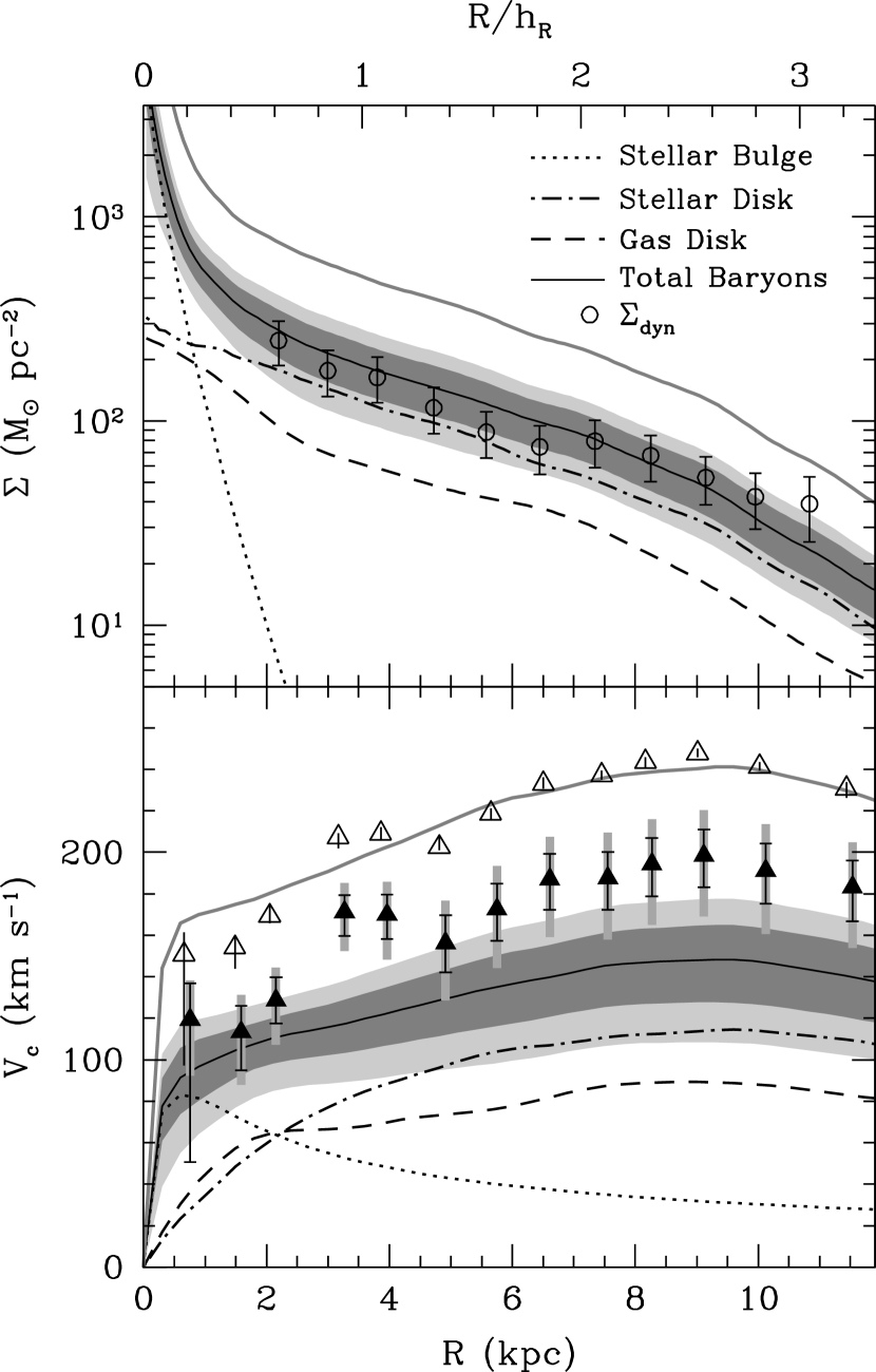
Figure 14.— Mass-surface-density (top) and circular-speed (bottom) distributions for the stellar bulge (dotted line), stellar disk (dot-dashed line), gaseous disk (dashed line), and all baryonic matter (solid black line) in UGC 463 assuming a constant $\Upsilon_{\ast,K}(R)$. Our measurements of $\Sigma_{\rm dyn}$ at $R>2$ kpc are overplotted as open symbols in the top panel for reference, which are directly traced during our calculations assuming a variable $\Upsilon_{\ast,K}(R)$. Dark- and light-gray regions illustrate, respectively, the random and systematic error in $\Sigma_{\rm b}$ and $V_{\rm b}$. The solid gray lines assume $\Upsilon_{\ast,K}=\Upsilon_{\ast,K}^{\rm SPS}$ as predicted by B03. Measurements of the DM-only circular speed ($V_{\rm DM}$; black triangles) are calculated by subtracting $V_{\rm b}$ from $V_{\rm c}$ (open triangles) in quadrature. Random and systematic errors in $V_{\rm DM}$ are shown as black and gray error bars, respectively.

Due to our imposition of a constant $\Upsilon_{\ast,K}$ for the mass decomposition illustrated in Figure 14, the surface density of all baryonic mass components, $\Sigma_{\rm b}$, does not exactly follow our $\Sigma_{\rm dyn}$ measurements. We have also performed a more direct mass decomposition that adopts $\Sigma_{\rm b}=\Sigma_{\rm dyn}$ by applying a smooth interpolation for $\Upsilon_{\ast,K}(R)=\Upsilon_{\ast,K}^{\rm disk}(R)$ at $2<R<11$ kpc; we extrapolate by simply extending the $\Upsilon_{\ast,K}^{\rm disk}$ measurements at the two endpoints of this range to small and large radius. This approach does not produce statistically different values for the quantities discussed below. For completeness, Table 8 provides the implied DM properties for both a constant and variable $\Upsilon_{\ast,K}(R)$; however, we simplify the discussion below by primarily focusing on the results obtained by assuming a constant $\Upsilon_{\ast,K}(R)$. This approach is justified by the consistency of our measurements with a radially invariant $\Upsilon_{\ast,K}^{\rm disk}$ as discussed in Section 5.6.2.

In addition to the constant $\Upsilon_{\ast,K}$ based on our dynamical measurements, Figure 14 also provides the calculation of $\Sigma_{\rm b}$ and $V_{\rm b}$ assuming $\Upsilon_{\ast,K}=\Upsilon_{\ast,K}^{\rm SPS}=0.79$, based on the prediction of B03; adopting the Z09 prediction produces $V_{\rm b}$ within the systematic errors of our dynamical measurements. The stellar and baryonic mass are, thereby, increased by a factor of 3.6 and 2.7, respectively, resulting in a maximal disk (i.e., $V_{\rm b}\sim V_{\rm c}$). Therefore, we can account for the measured rotation velocity within $R\leq 3.2h_{R}$ by simply scaling $\mu^{\prime}_{K}$ by a constant $\Upsilon_{\ast,K}$. This result is not unexpected given that the “diet Salpeter” IMF, used by B03, was chosen by Bell & de Jong (2001) to accommodate the “maximum-disk” rotation-curve mass decompositions produced by Verheijen (1997). Moreover, this is consistent with the expectation from most rotation-curve mass decompositions in the literature performed within similar radial regimes (see discussion by Sancisi, 2004), including the recent study of dwarf galaxies performed by Swaters et al. (2011). However, we have shown in Section 5.6 that the assumption $\Upsilon_{\ast,K}=\Upsilon_{\ast,K}^{\rm SPS}=0.79$ is rejected by our $\Upsilon_{\ast,K}^{\rm disk}$ measurements at $\gg 99$% confidence. That is, while it is possible to account for the rotation curve of UGC 463 within $R\leq 3.2h_{R}$ without invoking DM, DM is effectively required by our treatment of the observed stellar kinematics and, in fact, dominates the mass budget (Section 6.3.3). Moreover, the implied DM-mass distribution must be substantially less oblate than the baryonic-mass (disk) distribution traced by our stellar kinematics to simultaneously explain our measurements of $V_{\rm c}$ and $\overline{\sigma_{\ast}}$, as discussed in Section 5.6.2.

We note here that the DM properties we infer below are robust against many of the assumptions made above concerning the detailed baryonic mass decomposition. First, our characterization of the intrinsic central light concentration is a marginal consideration for calculating $V_{\rm b}$. For the innermost measurement of $V_{\rm c}$ ($R=0.7$ kpc), $V_{\rm b}$ is 10% (9.1 km s^-1) higher for our nominal measurement than if we were to adopt the stellar-disk density distribution at all radii; the random errors are 15%. This difference increases to 25% (23.3 km s^-1) if we also omit the instrumental-smoothing correction to $\mu^{\prime}_{K}$; however, the difference at the radius of the second measurement of $V_{\rm c}$ (at $R=1.5$ kpc) in this case is only 2% (3.5 km s^-1). Second, we find statistically equivalent measurements of the DM rotation speed, $V_{\rm DM}$, when simply calculating $V_{\rm b}$ directly from $\Sigma_{\rm b}=\Sigma_{\rm dyn}$ and assuming the nominal oblateness of the disk. The detailed baryonic mass decomposition presented here is meant to couch our rotation-curve mass decomposition within the traditional construct found in the literature and to provide insight into the baryonic mass budget of UGC 463.

6.2. Dark-Matter-Halo Circular Speed, Mass, and Volume Density

Figure 14 provides measurements of $V_{\rm DM}^{2}=V_{\rm c}^{2}-V_{\rm b}^{2}$ assuming a constant $\Upsilon_{\ast,K}(R)$; the enclosed mass of the presumed spherical halo is $\mathcal{M}^{\rm halo}_{\rm DM}=(8.9^{+1.3}_{-1.6}\ {}^{+2.1}_{-2.9})\times 10^{10}\mathcal{M}_{\odot}$ within the radial range of our measurements ($R\leq 11.4$ kpc). Measurements of $V_{\rm DM}$ also provide the spherical-halo volume-density profile via

$$\rho_{\rm DM}=\frac{V_{\rm DM}^{2}}{4\pi GR^{2}}\left(1+\frac{d\ln V_{\rm DM}^{2}}{d\ln R}\right)$$ (15)

(de Blok et al., 2001; Swaters et al., 2003a) as shown in Figure 15, where we calculate $dV_{\rm DM}^{2}/dR=dV_{\rm c}^{2}/dR-dV_{\rm b}^{2}/dR$ based on the model values for $V_{\rm c}$ and $V_{\rm b}$. The calculation of $dV_{\rm c}/dR$ is the same as used in Section 5.5 to calculate $\kappa$, and the calculation of $dV_{\rm b}/dR$ is done via finite-differencing of the $V_{\rm b}$ data in Figure 14. Measurements of $\rho_{\rm DM}$ are upper limits at $R\gtrsim 4$ kpc ($R\gtrsim 1.1h_{R}$) because the random error, $\epsilon(\rho_{\rm DM})$, becomes larger than the measured value.

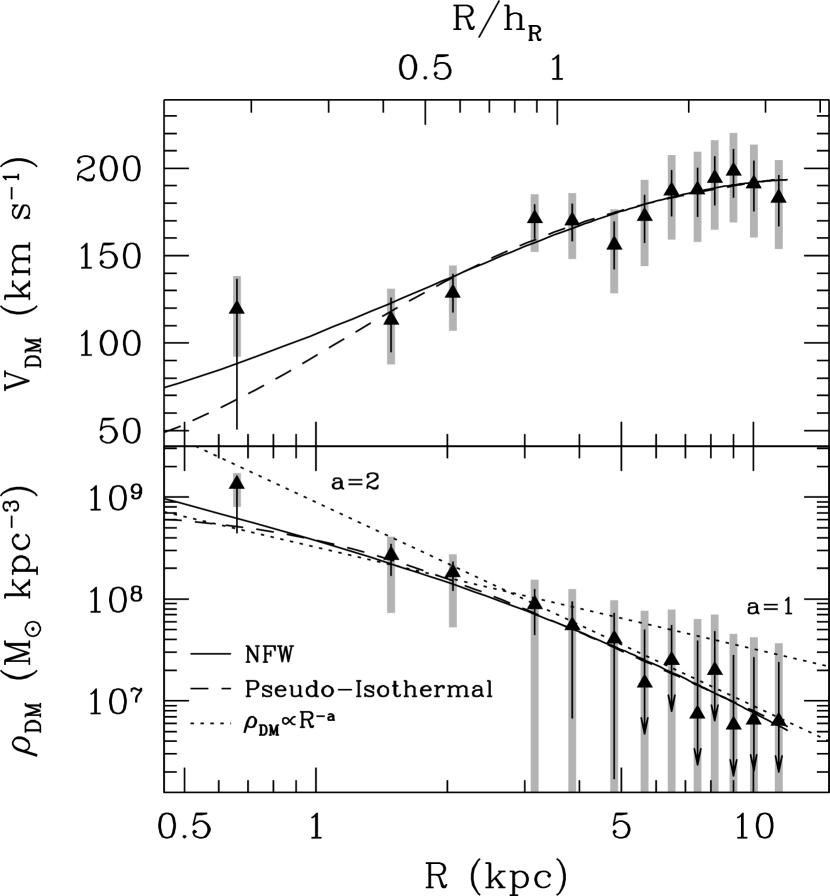
Figure 15.— The DM-only circular speed ($V_{\rm DM}$; top) and volume-density profile ($\rho_{\rm DM}$; bottom) for UGC 463 assuming a constant $\Upsilon_{\ast,K}(R)$; random and systematic errors are shown in black and gray, respectively. Upper limit arrows are used for data with random errors of $\epsilon(\rho_{\rm DM})>\rho_{\rm DM}$. The best-fitting NFW (solid lines) and pseudo-isothermal (dashed lines) parameterizations of the DM-halo are shown against the data. For reference, dotted lines in the bottom panel provide simple power-law density distributions following $\rho_{\rm DM}\propto R^{-a}$ for $a=1$ and 2; zero-points are set to approximately match the trend at small and large radius for $a=1$ and $a=2$, respectively.

We model the $V_{\rm DM}$ data in Figure 15 using a spherical “NFW” halo (Navarro et al., 1996, 1997) and a pseudo-isothermal sphere (Ostriker & Caldwell, 1979; Schmidt, 1985; Kent, 1986). The former is parameterized by the total halo mass, $\mathcal{M}^{\rm halo}_{\rm DM}$, and its concentration $c=R_{200}/R_{s}$, where $R_{200}$ is the radius at which the halo reaches 200 times the critical density ($\rho_{\rm crit}=3H_{0}^{2}/8\pi G$) and $R_{s}$ is the characteristic scale of the density profile; as above, we adopt $H_{0}=73$ km s^-1 Mpc^-1. The pseudo-isothermal sphere is parameterized by its central density, $\rho_{0}$, and core radius, $R_{c}$. Best-fitting DM halo parameters are determined by $\chi^{2}$-minimization, where $\chi^{2}$ is defined using only the random errors. Bootstrap simulations are used to calculate the random error in each the parameter. Systematic errors are based on 100 simulations of refitting the DM halo after MC sampling of the systematic errors in $V_{\rm DM}$, again minimizing a $\chi^{2}$ incorporating only the random errors. The best-fitting DM halo models are plotted against our measurements in Figure 15; we provide the best-fitting parameters for both a constant and variable $\Upsilon_{\ast,K}(R)$ in Table 8. Statistically, the NFW and pseudo-isothermal halos are equally suitable descriptions of the DM halo of UGC 463, and there is only a marginal difference between the results when using a constant or variable $\Upsilon_{\ast,K}(R)$. While the reduced $\chi^{2}$ is lower when adopting a constant $\Upsilon_{\ast,K}(R)$, the systematic deviations of the data about the model is such that this difference is not statistically meaningful. For comparison, Figure 15 also shows simple power-law density profiles following $\rho_{\rm DM}\propto R^{-a}$ for $a=1$ and 2; zero-points have been set by-eye in each case.

Table 8UGC 463 DM-Halo Properties

Parameter		Constant $\Upsilon_{\ast,K}$	Variable $\Upsilon_{\ast,K}$
Pseudo-Isothermal:	$\log\rho_{0}$	$8.85\pm 0.21\pm 0.13$	$8.83\pm 0.16\pm 0.09$
	$R_{c}$	$1.06\pm 0.21\pm 0.01$	$1.16\pm 0.21\pm 0.04$
	$\chi^{2}_{\nu}$	0.64	1.20
NFW Halo:	$\log\mathcal{M}^{\rm halo}_{\rm DM}$	$11.51\pm 0.09\pm 0.15$	$11.60\pm 0.09\pm 0.07$
	$c$	$19.2\pm 2.7\pm 1.6$	$18.9\pm 2.7\pm 1.2$
	$\chi^{2}_{\nu}$	0.61	1.14
	$\mathcal{F}_{\rm b}(R_{e})$	$0.81^{+0.48}_{-0.15}\ {}^{+0.24}_{-0.35}$	$0.78^{+0.43}_{-0.13}\ {}^{+0.17}_{-0.22}$
	$\mathcal{F}_{\rm b}(2.2h_{R})$	$0.61^{+0.07}_{-0.09}\ {}^{+0.12}_{-0.18}$	$0.53^{+0.05}_{-0.07}\ {}^{+0.09}_{-0.12}$
	$\mathcal{F}_{\ast}^{\rm disk}(2.2h_{R})$	$0.46^{+0.09}_{-0.12}\ {}^{+0.15}_{-0.22}$	$0.36^{+0.08}_{-0.10}\ {}^{+0.11}_{-0.15}$

We measure the concentration of the NFW halo to be $c=19^{+3}_{-2}$ in reasonable agreement with the expectation for low-redshift DM halos of similar mass (Navarro et al., 1997; Bullock et al., 2001). Thus, consistent with our measurement of a relatively low-mass disk, it appears that the baryons have had little effect on the structure of the DM halo. However, it is difficult to assess the physical meaning of this concentration index given the simplicity of our halo fitting; specifically, we do not include adiabatic contraction, which should be a relatively small effect given the expected gravitational influence of the baryons. It is interesting that the innermost $\rho_{\rm DM}$ datum indicates a steeper slope than provided by either of the DM-halo parameterizations, demonstrating $a\sim 2$ as opposed to unity. However, the error in this measurement is large and is highly subject to our treatment of the central mass concentration. The full DMS sample will provide stronger statistical constraints on the inner halo profile.

6.3. The Dominant Gravitational Influence of Dark Matter

As discussed in Section 1, assessments of the relative contribution of dark and baryonic matter to disk-galaxy mass budgets have been limited by the disk-halo degeneracy (van Albada et al., 1985). We have measured these contributions directly for UGC 463. Although allowing for a novel investigation of the DM mass distribution, it is useful to cast our analysis also in terms of a traditional approach such that we can compare with previous studies.

In particular, a common praxis in rotation-curve mass decomposition is the so-called “maximum-disk” hypothesis (vAS86), producing an extremum of the mass budget. Application of the “maximum-disk” hypothesis amounts to maximizing a radially independent mass-to-light ratio while adjusting any DM-halo parameters to fit the observed circular speed; however, exact implementations have varied. All baryonic components have been approximated by a single exponential disk (as in van Albada et al., 1985), values of $\Upsilon_{\ast}$ have been distinct (as in, e.g., Kent, 1986, 1987) or identical (as done above) for the bulge and disk components; and the gas disk has been subsumed into or isolated from the stellar component(s). Thus, one should keep in mind that, although termed the “maximum-disk” hypothesis, the direct association of this hypothesis with the stellar disk, in particular, can be tenuous in its practical implementation. Regardless, all implementations minimize the DM contribution to the mass budget at small radius. Galaxies adhering to the “maximum-disk” hypothesis are often said to have maximal disks; however, this definition remains inchoate.

The “maximality” of a galaxy is often assessed via the stellar-disk mass fraction, $\mathcal{F}_{\ast}^{\rm disk}=V^{\rm disk}_{\ast}/V_{\rm c}$ (equation 11 in Paper II, ). This quantity is traditionally measured at $2.2h_{R}$, the radius at which the circular speed peaks for razor-thin, radially exponential disks (see the generalization to oblate disks in Paper II, ). In the idealized case of a two-component galaxy with a spherical DM halo and an exponential stellar disk, $\mathcal{F}_{\ast}^{\rm disk}(R=2.2h_{R})$ uniquely quantifies the influence of the DM on the mass budget at all radii for a given disk scale length, oblateness, and DM-halo density parameterization. This idealized case provides a useful fiducial model with which to compare observations, as we discuss below. Real galaxies deviate from the idealized case due to (1) the inclusion of other baryonic components with generally different mass distributions, such as bulges and gaseous disks, and (2) perturbations of the stellar-disk mass-surface-density profile away from the nominal exponential, as inferred from surface-brightness variations. Thus, as explicitly associated with the stellar disk, $\mathcal{F}_{\ast}^{\rm disk}(R=2.2h_{R})$ has an intrinsic distribution for maximal disks: Sackett (1997) adopted $\mathcal{F}_{\ast}^{\rm disk}(R=2.2h_{R})=0.85\pm 0.10$ as an appropriate definition for maximal disks in galaxies of similar Hubble type to the Milky Way (Sb to Sc), also representative of the DMS Phase-B sample. We directly compare this definition to our measurements in UGC 463; however, we note that the literature studies upon which this definition was based do not remove the molecular gas component from the total disk mass distribution as we do for UGC 463.

As roughly synonymous throughout the discussion by vAS86, the “maximum-disk” hypothesis could also be termed the “maximum-baryon” or “minimum-dark-matter” hypothesis. In this respect, it is also useful to calculate the baryonic mass fraction, $\mathcal{F}_{\rm b}=V_{\rm b}/V_{\rm c}$. As implemented by vAS86, $\mathcal{F}_{\rm b}\approx\mathcal{F}_{\ast}^{\rm disk}$ at least in the sense that their mass-to-light ratios incorporated all mass distributed similarly to the luminous disk and they assumed the stellar disk was by far the most massive baryonic component. Our detailed accounting of multiple baryonic components in UGC 463 with different mass distributions, particularly with regard to the massive gas disk, means that (1) $\mathcal{F}_{\rm b}\neq\mathcal{F}_{\ast}^{\rm disk}$ and (2) quoting $\mathcal{F}_{\ast}^{\rm disk}(2.2h_{R})$ has a more limited bearing on the relative influence of the baryonic and DM mass on the total mass budget than described above. Therefore, it is useful to consider the radial functions $\mathcal{F}_{\ast}^{\rm disk}(R)$ and $\mathcal{F}_{\rm b}(R)$ and to define multiple fiducial radii for $\mathcal{F}_{\rm b}$ based on the expectation of that each baryonic component can dominate the mass budget in distinct radial regimes.

One expects $\mathcal{F}_{\rm b}$ to decrease with radius as DM increasingly dominates the mass budget. The “maximum-disk” hypothesis effectively states $\mathcal{F}_{\rm b}\sim 1$ at small radius, regardless of whether or not the disk or bulge dominates the baryonic mass (see the implementation of the “maximum-disk” hypothesis by, e.g., Kent, 1986, 1987). The application of $\mathcal{F}_{\rm b}\sim 1$ at small radius to Sb–Sc galaxies has shown $\mathcal{F}_{\ast}^{\rm disk}(2.2h_{R})=0.85$, which may be considered a lower limit for $\mathcal{F}_{\rm b}$ at these radii. Finally, it is expected that $\mathcal{F}_{\rm b}\to 0$ at large radius because rotation curves have been shown to remain nearly constant up to the radial extent of H i disks. The recent study by Dutton et al. (2011b) has shown that this expectation for $\mathcal{F}_{\rm b}(R)$ is likely a limited picture of the range in galaxy properties. By combining strong lensing analysis and stellar kinematics, Dutton et al. have shown $\mathcal{F}_{\rm b}(R_{e})=0.99$ and $\mathcal{F}_{\rm b}(2.2h_{R})=0.67$ for the late-type lens galaxy SDSS J2141-0001, which is at a redshift of 0.14; $R_{e}$ is the effective (half-light) radius of the bulge (Section 2.2.2). Thus, while adhering to the fundamental tenant of the “maximum-disk” hypothesis, SDSS J2141-0001 exhibits a disk that is relatively less massive than the disks of local Sb–Sc galaxies, such that it would be considered “submaximal” under the definition proposed by Sackett (1997).

For UGC 463, we assess the ratio of the dark and baryonic mass components via the mass fractions $\mathcal{F}_{\ast}^{\rm disk}$ and $\mathcal{F}_{\rm b}$ in Section 6.3.1. We quote $\mathcal{F}_{\rm b}$ at $R_{e}=0.5$ kpc and $2.2h_{R}=7.8$ kpc as to compare with both the expectations from the “maximum-disk” hypothesis and the results from Dutton et al. (2011b). These radii are close to the radii at which the circular speeds of the stellar components are maximized (Figure 14). We also quote $\mathcal{F}_{\ast}^{\rm disk}(2.2h_{R})$ for a direct comparison with the definition of a maximal disk proposed by Sackett (1997). Further assessments are made using the ratio of the mid-plane volume densities $(\rho_{\rm DM}/\rho_{\rm b})_{z=0}$ in Section 6.3.2 and the enclosed-mass budget in Section 6.3.3. In all of these sections, we compare our measurements for UGC 463 with an idealized, maximal-disk galaxy; this model provides the equivalent quantities for a maximal disk that has been embedded in the NFW and pseudo-isothermal halos fitted to our measurements of $V_{\rm DM}$ (Section 6.2). This fiducial maximal disk has the scale length and oblateness as measured for UGC 463, is purely exponential in both $R$ and $z$ and has $\mathcal{F}_{\rm disk}=0.85$ at $R=2.2h_{R}$. Here, our notation $\mathcal{F}_{\rm disk}$, as opposed to $\mathcal{F}_{\ast}^{\rm disk}$, purposely leaves the nature of the matter in the disk undefined, as done by vAS86 in their implementation of the “maximum-disk” hypothesis. The combination of this fiducial maximal disk and our fitted DM halos produces a substantially higher circular speed than we measure for UGC 463, and the shape of the rotation curve does not adhere to the disk-halo conspiracy (vAS86); we have shown in Section 6.1 that application of the “maximum-disk” hypothesis to UGC 463 essentially results in a marginal DM-halo mass within the radial regime probed by our data.

Before continuing, we note that Bottema (1993, 1997) used kinematic measurements similar to our own and found $\mathcal{F}_{\rm disk}(2.2h_{R})=0.63\pm 0.10$ for a sample of 12 late-type galaxies; Bottema did not differentiate between stellar and gas components in this decomposition, hence our use of $\mathcal{F}_{\rm disk}$. In detail, Bottema’s assumptions are not exactly the same as our own; however, we can cast UGC 463 in terms of his measurement to find $\mathcal{F}_{\rm disk}(2.2h_{R})=0.6$, which is compatible with these previous results. We also note that, using planetary nebulae as kinematic tracers, Herrmann & Ciardullo (2009) reported submaximal disks for four of the five galaxies they studied.

6.3.1 Stellar-Disk and Baryonic Mass Fractions, $\mathcal{F}_{\ast}^{\rm disk}$ and $\mathcal{F}_{\rm b}$

Figure 16 provides $\mathcal{F}_{\ast}^{\rm disk}$ and $\mathcal{F}_{\rm b}$ as a function of radius assuming a constant $\Upsilon_{\ast,K}(R)$. Individual data points use our direct measurements of $V_{\rm c}$, whereas the gray lines calculate $V_{\rm c}^{2}=V_{\rm b}^{2}+V_{\rm DM}^{2}$ using $V_{\rm b}$ from Figure 14 and $V_{\rm DM}$ from the NFW and pseudo-isothermal halos fitted in Figure 15. Both $\mathcal{F}_{\ast}^{\rm disk}(R)$ and $\mathcal{F}_{\rm b}(R)$ are effectively constant between $1.0\lesssim R/h_{R}\lesssim 3.5$; the roughly constant $\mathcal{F}_{\rm b}-\mathcal{F}_{\ast}^{\rm disk}$ at these radii reflects the similarity between the radial distribution of the gas and stars. Figure 16 also provides the expected $\mathcal{F}_{\rm disk}$ for the fiducial maximum disk, which is the same for the NFW and pseudo-isothermal halos at $R\gtrsim 0.5h_{R}$. The shape of $\mathcal{F}_{\ast}^{\rm disk}(R)$ is very similar to that calculated for a maximal disk, which is essentially a statement that $\mu^{\prime}_{K}$ is very close to an exponential after subtracting the central light concentration; however, the normalization is very different. At small radius, $\mathcal{F}_{\rm b}$ and $\mathcal{F}_{\ast}^{\rm disk}$ diverge largely due to the exclusion of the central mass concentration in the calculation of the latter.

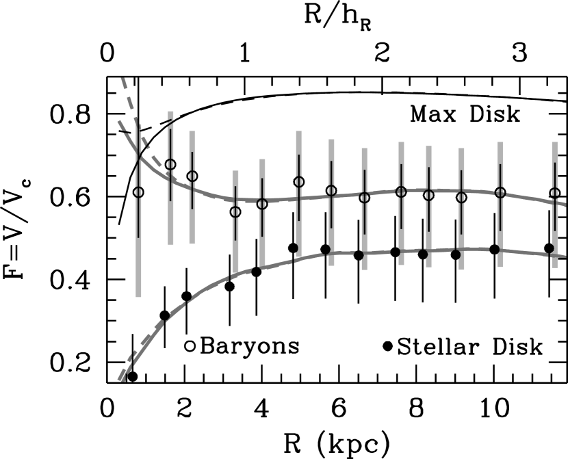
Figure 16.— Mass fractions ($\mathcal{F}=V/V_{\rm c}$) of the stellar disk ($\mathcal{F}_{\ast}^{\rm disk}$; filled points) and all baryonic matter ($\mathcal{F}_{\rm b}$; open circles) as a function of radius assuming a constant $\Upsilon_{\ast,K}(R)$. The discrete measurements use the measured values of $V_{\rm c}$; random errors are shown in black for both quantities, whereas systematic errors are shown in gray only for measurements of $\mathcal{F}_{\rm b}$. Gray lines show the result of calculating $V_{\rm c}^{2}=V_{\rm DM}^{2}+V_{\rm b}^{2}$ using the NFW (solid gray lines) and pseudo-isothermal (dashed gray lines) DM halo models from Figure 15. Black lines show $\mathcal{F}_{\rm disk}$ for a fiducial maximal disk ($\mathcal{F}_{\rm disk}=0.85$ at $R=2.2h_{R}$) that has been embedded in the fitted DM halos (see text).

Table 8 gives $\mathcal{F}_{\rm b}(R_{e})$, $\mathcal{F}_{\rm b}(2.2h_{R})$, and $\mathcal{F}_{\ast}^{\rm disk}(2.2h_{R})$ for both the constant and variable $\Upsilon_{\ast,K}(R)$ assumptions. Our measurement of $\mathcal{F}_{\rm b}(R_{e})$ has significant uncertainty due to the error in measurement of $V_{\rm c}$ at this radius (largely due to centering errors), the uncertainty in the baryonic rotation speed, and the difference in the extrapolation when based on either the NFW or pseudo-isothermal halo. To the contrary, both $\mathcal{F}_{\rm b}$ and $\mathcal{F}_{\ast}^{\rm disk}$ at $2.2h_{R}$ are relatively well constrained. Following the definition proposed by Sackett (1997) and assuming a constant $\Upsilon_{\ast,K}(R)$, these quantities demonstrate that UGC 463 has a substantially submaximal disk by a factor of $\sim(0.85/0.46)^{2}\approx 3.4$ in mass; this reduces to 1.9 if one instead defines $\mathcal{F}_{\rm b}(2.2h_{R})=0.85$ as a maximal disk. These factors are consistent with our previous discussion in Sections 5.6.2 and 6.1 regarding the comparison of our dynamical measurements with the SPS predictions from B03. Adopting a variable $\Upsilon_{\ast,K}(R)$ results in a mass profile of the disk that yields a peak rotation speed at or beyond the limit of our calculation ($R=15$ kpc), whereas the constant $\Upsilon_{\ast,K}(R)$ disk has a peak rotation at $2.7h_{R}$. However, in both cases the stellar (and baryonic) disk remains submaximal due to the relatively constant value of $\mathcal{F}_{\ast}^{\rm disk}$ (and $\mathcal{F}_{\rm b}$) at $R>h_{R}$. Although it is possible that the baryonic mass is close to satisfying the $\mathcal{F}_{\rm b}(R_{e})\sim 1$ given the uncertainty, our data suggest that the circular speed may have substantial contributions from DM even within the bulge region.

6.3.2 Mid-Plane Volume-Density Ratio, $(\rho_{\rm DM}/\rho_{\rm b})_{z=0}$

Our mass-surface-density and $\rho_{\rm DM}$ measurements from Figures 14 and 15, respectively, provide the mid-plane volume-density ratio between the dark and baryonic matter, $(\rho_{\rm DM}/\rho_{\rm b})_{z=0}$. We assume that the stratification of the gaseous and stellar disks combine to produce an exponential vertical density distribution with a single scale height $h_{z}$ and that the bulge is spherical. Thus, the baryonic volume density at the disk mid-plane is $(\rho_{\rm b})_{z=0}=(\Sigma_{\rm\ast}+\Sigma_{\rm gas})/2h_{z}+\rho_{\rm bulge}$. If the gas is more confined to the plane, this calculation results in upper limits. Figure 17 provides the mid-plane volume-density ratio when assuming a constant $\Upsilon_{\ast,K}(R)$, where the discrete measurements use the non-parametric calculation of $\rho_{\rm DM}$ and the gray lines use the NFW and pseudo-isothermal sphere parameterizations. We also plot the expectation for the fiducial maximal disk discussed above. For reference, Bienaymé et al. (2006) find $(\rho_{\rm DM}/\rho_{\rm b})_{z=0}=0.14$ in the solar neighborhood assuming a spherical halo.

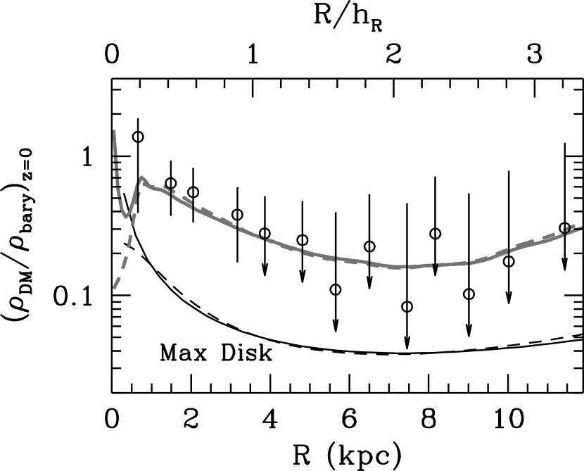
Figure 17.— Mid-plane density ratio $(\rho_{\rm DM}/\rho_{\rm b})_{z=0}$ of all baryonic matter as a function of radius assuming a constant $\Upsilon_{\ast,K}(R)$. The calculation of $(\rho_{\rm b})_{z=0}$ is discussed in the text. Data points use the $\rho_{\rm DM}$ measurements from Figure 15, whereas gray lines use the NFW (gray solid lines) and pseudo-isothermal (gray dashed lines) parameterizations of $\rho_{\rm DM}$. Only random errors are shown; upper limit arrows are used when the error is larger than the measured value. The results for the fiducial maximal disk are plotted as black lines for both the NFW (solid black lines) and pseudo-isothermal (dashed black lines) DM halo parameterizations.

At $R\gg z$, the change in $\rho_{\rm DM}$ with $z$ is much smaller than the change in $\rho_{\rm b}$ such that $(\rho_{\rm DM}/\rho_{\rm b})\propto\exp(|z|/h_{z})$. Averaging the data at $1<R/h_{R}<3$ in Figure 17, we find that $(\rho_{\rm DM}/\rho_{\rm b})_{z=0}\sim 0.2$, which is a factor of 5 larger than the expectation for a maximal disk (only 40% larger than the Milky-Way value). The mass volume density of UGC 463 is, therefore, dominated by dark matter at $|z|\gtrsim 1.6h_{z}$ at $R\gtrsim h_{R}$. This result is particularly important for our understanding of out-of-plane motions in the disk of UGC 463: The derivation of $\Sigma_{\rm dyn}=\sigma_{z}^{2}/\pi kGh_{z}$ assumes an isolated, plane-parallel, infinite disk. Deviations from these assumptions, such as embedding the disk in a very massive DM halo, introduces systematic errors in the calculation, as briefly discussed in Paper II. The result for $(\rho_{\rm DM}/\rho_{\rm b})_{z=0}$ in UGC 463 suggests that such effects may be significant for this galaxy.

Bottema (1993) has discussed the influence of a massive DM halo on $\sigma_{z}$ in disk stars, continuing the work of Bahcall (1984). These authors find that $\sigma_{z}$ should be inflated relative to an isolated disk when embedded in a massive, spherical halo; the degree of the inflation is proportional to $(\rho_{\rm DM}/\rho_{\rm b})_{z=0}$, as shown in Figure 15 from Bottema (1993). For the fiducial maximal disk shown in our Figure 17, Bottema (1993) would predict a less than 5% increase in the $\sigma_{z}$ over an isolated disk, whereas our measurements for UGC 463 from Figure 17 suggest $\sigma_{z}$ could be increased by $10-15$%. This means that our calculation of $\Sigma_{\rm dyn}\propto\sigma_{z}^{2}$ could overestimate the mass of the disk by $20-30$%.

Ideally, one would calculate $\Sigma_{\rm dyn}$ by first assuming an isolated disk and then converging to a solution that incorporated the effects of the DM halo. However, we have not done so here for UGC 463 because (1) the random error in our isolated-disk measurements of $\Sigma_{\rm dyn}$ are of the same order as this systematic correction; (2) there is substantial error in our measurement of $(\rho_{\rm DM}/\rho_{\rm b})_{z=0}\sim 0.2$, even if we adopt the parameterized solutions for $\rho_{\rm DM}$; and (3) there are equally unknown competing systematics that work in the opposite direction, such as the inclusion of a massive, razor-thin gas disk. The continued study of the effects of a massive halo on the velocity dispersion, as opposed to just the rotation curve (Hayashi & Navarro, 2006; Widrow, 2008), is worthy of a dedicated effort. However, given ambiguities regarding the three-dimensional structure of galaxies and the vertical stratification of disks (see discussion in Section 5.6.1), a detailed understanding of the influence of the DM halo on the disk is complicated. Here, we simply note that the impact of a relatively massive DM halo in UGC 463 works to further lower the maximality of an already submaximal disk.

6.3.3 Enclosed-Mass Budget

As discussed in Paper II, the total baryon fraction ${\mathcal{F}}_{\rm bar}=\mathcal{M}^{\rm tot}_{\rm b}/\mathcal{M}^{\rm tot}_{\rm dyn}$ is ill-defined; however, the surface density and $V_{\rm DM}$ measurements from Figure 14 allow for a robust calculation of the enclosed-mass budget to a finite radius, assuming the halo is spherical. The resulting mass budget is presented in Table 7 and the mass growth curves are shown in Figure 18. We end the calculation at $R=15$ kpc ($R=4.2h_{R}$; $\sim R_{200}/10$ for our fitted NFW halo), well within the limiting radius of our $\mu^{\prime}_{K}$ measurements (Figure 2) but extrapolating beyond our dynamical data. We calculate the DM mass at 15 kpc using the fitted halo parameterizations and the percentage errors from the measured data. The mass growth curve of the fiducial maximal disk discussed above is overplotted in Figure 18 for reference. Although Table 7 only provides the results when assuming a constant $\Upsilon_{\ast,K}(R)$, the results assuming a variable $\Upsilon_{\ast,K}(R)$ are insignificantly different.

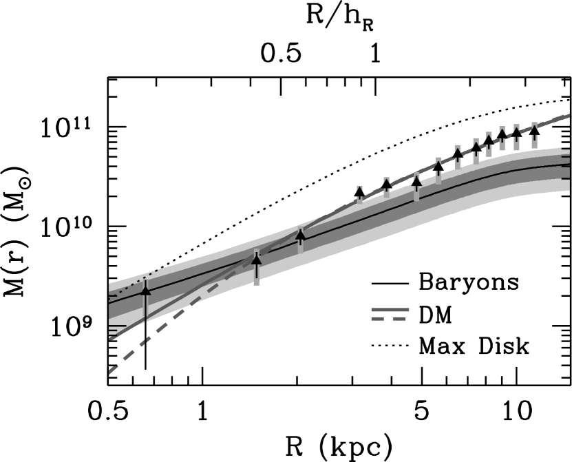
Figure 18.— Mass growth curves for baryonic mass (solid black line), NFW (gray solid line) and pseudo-isothermal (gray dashed line) DM halo parameterizations, and the fiducial maximal disk (dotted line). The baryonic mass profile assumes a constant $\Upsilon_{\ast,K}(R)$; the dark- and light-gray regions represent the random and systematic errors, respectively. Individual measurements of $V_{\rm DM}$ from Figure 15 are converted to masses assuming a spherical halo and plotted as black triangles; black and gray bars represent the random and systematic errors, respectively.

Figure 18 shows that the integrated baryonic mass of UGC 463 is, at most, equal to the integrated DM mass at $R\sim h_{R}$. Beyond this radius, the integrated DM mass quickly begins to dominate, such that $\mathcal{M}_{\rm b}/\mathcal{M}_{\rm DM}\sim 0.3$ at 15 kpc. To the contrary, the integrated mass of the fiducial maximal disk always dominates over the DM mass; the minimum mass ratio $\mathcal{M}_{\rm disk}/\mathcal{M}_{\rm DM}\sim 1.4$ is at $R=15$ kpc.

7. Summary

In this paper, we have presented a detailed case study of the dynamics and implied mass budget of the low-inclination, SABc galaxy UGC 463. We find the galaxy to be dominated by DM at nearly all radii, a classification usually reserved for low-surface-brightness galaxies whereas UGC 463 is $\sim 1$ magnitude above the Freeman (1970) mean central surface brightness (Paper I). The stellar disk of UGC 463 is submaximal by a factor of $\gtrsim 3$ in mass. Submaximal disks have been both indirectly (e.g. Courteau & Rix, 1999) or directly (Bottema, 1993; Herrmann & Ciardullo, 2009) measured in the past, and our results are consistent with these measurements. At present, this general result should be unaffected by systematic error, despite the albeit large number of assumptions. A summary of our analysis follows.

Our analysis of UGC 463 draws from nearly all of our survey data for this galaxy as collectively described in Section 2. We derive a distance of $D=59.67\pm 0.01\pm 4.15$ Mpc using the flow-corrected systemic velocity and $H_{0}=73\pm 5$ km s^-1 Mpc^-1. We derive optical and NIR surface brightness profiles from, respectively, archival SDSS and 2MASS data; we use the latter to calculate a total $K$-band magnitude of $m_{K}=9.32\pm 0.02$. Our photometry is corrected for Galactic extinction; internal extinction and dust emission are marginal considerations for our results. We also correct for instrumental smoothing of the surface brightness profile at small radius. Ionized-gas and stellar kinematics are derived using SparsePak and PPak IFS. Ionized-gas kinematics combine results from atomic emission lines near H$\alpha$ and the [O iii]$\lambda 5007$ line; kinematics are measured using single or double Gaussian line fits (as in Andersen et al., 2008). Stellar kinematics are derived from absorption lines with rest wavelengths between $\sim 492-522$nm using DC3 (Paper III) and a single K1 III template star (HD 167042 for SparsePak and HD 162555 for PPak); template mismatch is $\lesssim 5$% (Paper II). All kinematics are corrected for instrumental broadening. We measure H i mass surface densities and the H i velocity field using 21cm aperture synthesis imaging from the VLA. Finally, we estimate the H₂ mass surface density by combining 24$\mu$m Spitzer imaging and a $I_{24\mu{\rm m}}/I_{\rm CO}\Delta V$ calibration based on our reanalysis of data tabulated by L08. Errors in our measurements of $\Sigma_{\rm H_{2}}$ incorporate the systematic error in this calibration and the error in our adopted value of $X_{\rm CO}=(2.7\pm 0.9)\times 10^{20}$ cm^-2 (K km s^-1)^-1.

In Section 3, we determine the detailed on-sky geometric projection of the disk of UGC 463, including extensive tests of the inclination. These efforts are important to subsequent analysis of the measured kinematics due to the substantial influence of inclination errors on the fundamental calculations in this study (Paper II). Inclinations are measured both kinematically — using an algorithm explained in Andersen et al. (2008) that assumes circular motion and a single, coplanar disk — and by inverting the TF relations from V01. Kinematic inclinations are most consistent between all ionized-gas and stellar tracers when adopting a $\partial V_{\rm LOS}/\partial i$ weighting scheme, as explained in Appendix B. We find $i_{\rm kin}=25\fdg 1\pm 2\fdg 5$ and $i_{\rm TF}=29\arcdeg\pm 2\arcdeg$; a combined measurement of $i=27\arcdeg\pm 2\arcdeg$ represents our best estimate for the inclination and is used throughout all subsequent analysis. We derive the dynamical center of each SparsePak observation and, for the PPak data, we affix the dynamical center to the morphological center determined from a reconstructed continuum map; our two-dimensional maps in Figure 1 demonstrate that the dynamical and morphological centers of UGC 463 are identical to within the errors of our measurement ($\sim 1\arcsec$).

Using the derived geometry, we create azimuthally averaged kinematics in Section 4. To combine kinematic measurements using different instruments and different wavelength regimes, we apply beam-smearing corrections to both our ionized-gas and stellar kinematics; beam-smearing corrections to the H i data are described by Martinsson (2011). The beam-smearing corrections employ model surface-brightness, velocity, and velocity-dispersion distributions to create a synthetic dataset that is compared to our observations; the corrections are small (less than a few percent) except for data near the dynamical center. Figure 7 demonstrates that both the ionized-gas and stellar kinematics measured separately by SparsePak and PPak are very well matched. We provide a cursory assessment of the kinematic axisymmetry of the rotation curves and velocity dispersion profiles by overlaying $180\arcdeg$ azimuthally averaged kinematics for the receding and approaching sides in Figure 7; with respect to the errors, only moderate differences are present. Therefore, we impose axisymmetry by measuring the gas (ionized$+$neutral) and stellar velocity and velocity dispersions only as a function of in-plane galaxy radius. We correct the gas rotation curve to the circular speed using measurements of $\sigma_{\rm gas}$ and $\Sigma_{\rm gas}$ following Dalcanton & Stilp (2010) to produce the axisymmetric radial profiles in Figure 8.

Based on our collection of azimuthally averaged properties, we determine physical properties of the disk of UGC 463 in Section 5. We find that the stellar velocity dispersion profile, $\overline{\sigma_{\ast}}(R)$, has only minor deviations from a pure exponential; the fitted $e$-folding length ($h_{\sigma}\sim 2.6h_{R}$) suggests either $\Upsilon_{\rm dyn}$ or $h_{z}$ increases by a factor of $\sim 2.3$ over the radial range of our data, if the other quantity is radially invariant. Using the measured circular speed, stellar rotation curve, and stellar velocity dispersion profile, we calculate the observable function $\delta_{\rm AD}(R)$. This function is directly related to the shape of the SVE such that we find $\alpha=0.48\pm 0.09$ and $\beta=1.04\pm 0.22$, when assumed to be constant over the entire disk. Therefore, we find the conversion factors $\sigma_{z}/\langle\sigma_{\ast}\rangle_{\theta}=0.76\pm 0.09$ and $\sigma_{R}/\langle\sigma_{\ast}\rangle_{\theta}=1.59\pm 0.17$, which we use in our calculations of $\Sigma_{\rm dyn}$ and the disk stability, $Q$. Our calculations of $\Sigma_{\rm dyn}$ (Figure 10) use equation 9 from Paper II, which assumes the oblateness from their equation 1. We find $\Sigma_{\rm dyn}$ is well fit by 3$\Sigma_{\rm gas}$, from which it follows that $\Sigma_{\rm\ast}\sim 2\Sigma_{\rm gas}$. Using $\Sigma_{\rm gas}$, $\sigma_{\rm gas}$, $\Sigma_{\rm\ast}$, and $\sigma_{R}$, we calculate individual and multi-component stability coefficients following from, respectively, Toomre (1964) and Rafikov (2001). We find the disk to be globally stable, with the multi-component stability asymptotically decreasing with radius to a value of $Q_{\rm R}\sim 2$. Based on combining stability arguments with swing-amplification theory (Toomre, 1981; Athanassoula et al., 1987), disks of a fixed rotation curve should exhibit higher spiral-arm multiplicity when the disk mass is decreased. This expectation is qualitatively consistent with our measurements of a submaximal disk and three-arm multiplicity in UGC 463; however, Paper V and Martinsson (2011) find submaximal disks regardless of spiral-arm multiplicity.

We calculate $\Upsilon_{\ast,K}^{\rm disk}$ using $\Sigma_{\rm\ast}$ and $\mu^{\prime}_{K}$ to find $\langle\Upsilon_{\ast,K}^{\rm disk}\rangle=0.22\pm 0.09^{+0.16}_{-0.15}\ \mathcal{M}_{\odot}/\mathcal{L}_{\odot}^{K}$ at $R>2$ kpc. Our measurements of $\langle\Upsilon_{\ast,K}^{\rm disk}\rangle$ are systematically lower than SPS model predictions ($\Upsilon_{\ast,K}^{\rm SPS}$) from B03 by a factor of $\sim 3.6$ and larger than the SPS modeling of Z09 by a factor of $\sim 1.8$. Based on an MC sampling of probability distributions assigned to each quantity in the calculation, we generate a composite (random$+$systematic error) probability distribution for $\Upsilon_{\ast,K}^{\rm disk}(R)$ and $\langle\Upsilon_{\ast,K}^{\rm disk}\rangle$. We find that the Z09 prediction are within our 68% confidence interval for $\langle\Upsilon_{\ast,K}^{\rm disk}\rangle$; in contrast, measurements of $\langle\Upsilon_{\ast,K}^{\rm disk}\rangle$ consistent with the B03 prediction occur for less than 1 in $10^{5}$ MC samples. Z09 attribute the disparity between their $\Upsilon_{\ast,K}^{\rm SPS}$ predictions and those from B03 to different treatments of the star-formation history and TP-AGB phases of stellar evolution. We also find a factor of $\sim 2$ increase in $\Upsilon_{\ast,K}^{\rm disk}$ with radius, which is not predicted by the SPS modeling. This feature may reflect a true increase in the $\Upsilon_{\ast,K}^{\rm disk}$, a flaring of the stellar disk, or a change in the relative dynamical influence of the halo, thick stellar disk, and/or razor-thin gas disk.

We discuss the mass budget of UGC 463 out to 15 kpc (4.2 $h_{R}$) in Section 6 using a traditional rotation-curve mass decomposition, which benefits from our unique and direct measurement of $\Upsilon_{\ast,K}^{\rm disk}$. Our primary discussion assumes a constant $\Upsilon_{\ast,K}(R)=\langle\Upsilon_{\ast,K}^{\rm disk}\rangle$; however, we also briefly discuss results obtained by assuming a variable $\Upsilon_{\ast,K}(R)=\Upsilon_{\ast,K}^{\rm disk}(R)$. Our mass decomposition also assumes that $h_{z}$ is constant with radius and that the galaxy is composed of four separable potentials (halo, stellar bulge, stellar disk, and gas disk). The total mass budget obtained by assuming a constant $\Upsilon_{\ast,K}(R)$ is provided in Table 7; assuming a variable $\Upsilon_{\ast,K}(R)$ produces results that are statistically identical.

We calculate the circular speed of each baryonic component in Section 6.1. We find that a maximal disk may be produced by adopting the $\Upsilon_{\ast,K}^{\rm SPS}$ prediction from B03, which amounts to increasing the stellar (baryonic) mass by a factor of 3.6 (2.7) above our measurements of $\langle\Upsilon_{\ast,K}^{\rm disk}\rangle$. However, this result is effectively excluded by our simultaneous measurements of $V_{\rm c}$ and $\overline{\sigma_{\ast}}$. Using our dynamical measurements, we produce $V_{\rm DM}^{2}=V_{\rm c}^{2}-V_{\rm b}^{2}$ and use these measurements to calculate $\rho_{\rm DM}$; both $V_{\rm DM}$ and $\rho_{\rm DM}$ assume a spherical halo. In Section 6.2, we fit $V_{\rm DM}$ with an NFW and pseudo-isothermal DM halo, and we find both to be statistically suitable descriptions of our measurements. The concentration of the NFW halo is consistent with expectations from DM-only simulations, implying that the halo structure has been relatively unaffected by the collapsed baryons. Our measurements of $\rho_{\rm DM}$ show a slope that may be steeper than both $\rho_{\rm DM}\propto 1/R$ and the slope predicted by either DM-halo parameterization; however, this result is highly dependent on the error-prone assessment of the baryonic mass within the central kpc. Results for additional galaxies in our Phase-B sample are required to place better statistical constraints on the shape of DM halos of local disk galaxies.

We discuss the dominant gravitational influence of DM over baryonic matter in UGC 463 in Section 6.3, as summarized in Tables 7 and 8. Assuming a constant $\Upsilon_{\ast,K}(R)$, we find the baryonic disk to be substantially submaximal with $\mathcal{F}_{\rm b}(2.2h_{R})=0.61^{+0.07}_{-0.09}\ {}^{+0.12}_{-0.18}$. Considering only the stellar disk and adopting $\mathcal{F}_{\ast}^{\rm disk}(2.2h_{R})=0.85\pm 0.10$ as the definition of a maximal disk (Sackett, 1997), UGC 463 is submaximal by a factor of $\sim(0.85/0.46)^{2}=3.4$ in mass, consistent with our expectation based on the difference between $\langle\Upsilon_{\ast,K}^{\rm disk}\rangle$ and the $\Upsilon_{\ast,K}^{\rm SPS}$ prediction from B03 (Section 6.1). We also compare our measurements of the baryonic component to a fiducial maximal disk (having $\mathcal{F}_{\rm disk}(2.2h_{R})=0.85$) resulting from embedding a purely exponential disk (with $h_{R}$ and $h_{z}$ as measured for UGC 463) in our fitted NFW and pseudo-isothermal DM halos. In the disk mid-plane, we find the ratio $(\rho_{\rm DM}/\rho_{\rm b})_{z=0}$ is a factor of five larger than expected by our fiducial maximal disk, which may lead to an overestimate of $\Sigma_{\rm dyn}$. Additionally, we find that the enclosed-mass of the galaxy is dominated by DM at $R\gtrsim h_{R}$, whereas the fiducial maximal disk dominates the enclosed-mass budget at all radii sampled by our observations. Finally, assuming a constant $\Upsilon_{\ast,K}(R)$, we find a baryonic-to-DM mass ratio of $0.31\pm 0.8^{+0.16}_{-0.14}$ for the mass enclosed within the central 15 kpc.

Although our results are for a single galaxy, an analysis of 30 galaxies in our sample demonstrate that all of these disks are comparably submaximal (Paper V; Martinsson, 2011). One can increase the maximality of these disks by changing the assumptions concerning the vertical mass distribution (quantified by the constant $k$) or the applied oblateness ($q$), as discussed in Sections 5.3 and 5.6.1; however, $k$ and $q$ would have to take on values that are effectively excluded by empirical constraints on the structural parameters of disk galaxies based on edge-on systems (e.g., Kregel, 2003). The recalibration of $\Upsilon_{\ast}$ based on these results has significant consequences for, e.g., our understanding of the baryonic mass of galaxies as a function of redshift and for the gravitational interplay between baryonic and dark matter in the process of galaxy formation.

Appendix A Surface-Brightness Calibration and Interpolation of IFU Data

The spectral-continuum surface-brightness maps in the H$\alpha$ and Mg i regions shown in Figure 1 are calibrated against SDSS imaging data, assuming that the dynamical center (Table 6) is the same as the morphological center.

The “model” flux in fiber $f$ measured from the CCD data is

$$C_{{\rm mod},f}={\rm dlog}\left[0.4(Z_{\rm fib}-Z_{\rm CCD})+\log I_{{\rm CCD},f}\right]A_{\rm fib}-S_{\rm fib},$$ (A1)

where $Z$ represents a magnitude zero-point and $I_{{\rm CCD},f}=(C_{{\rm CCD},f}-S_{\rm CCD})/A_{\rm CCD}$ represents the surface brightness in units of DN arcsec^-2 — determined by the total flux ($C$) within an aperture (of area $A$) with a sky background ($S$). The fiber aperture area, $A_{\rm CCD}\sim A_{\rm fib}\equiv\pi D_{\rm fib}^{2}/4$, is known and the quantities related to the CCD image are measured or provided by the SDSS calibration. The fiber-continuum zero-point, $Z_{\rm fib}$, and sky-level, $S_{\rm fib}$, are free parameters; $S_{\rm fib}$ is fiber independent, adjusting the nominal correction based on the average sky spectrum. Equation A1 is fit to our IFS data by minimizing $(\sqrt{C_{{\rm fib},f}}-\sqrt{C_{{\rm mod},f}})^{2}$, where $C_{{\rm fib},f}$ is the mean flux across the full spectral range; data with erroneous negative flux are ignored. We also limit the radial region considered to avoid inflated errors were the sky subtraction of the IFS is particularly problematic due to variations in the sky flux as measured by the dedicated sky fibers.

We use the SDSS $g$-band ($1\farcs 5$ seeing) and $r$-band ($1\farcs 2$ seeing) data to calibrate the Mg i-region and H$\alpha$-region IFS, respectively. For the PPak data, analysis of guide-camera images taken throughout each exposure show that the average seeing was $1\farcs 7$ (Martinsson, 2011); therefore, we match this seeing by applying a Gaussian kernel with a FWHM of $0\farcs 8$ to the $g$-band image when fitting to the PPak data. No such seeing measurements are available for the SparsePak data. Although we have allowed the seeing to be a fitted parameter for SparsePak, seeing measurements were non-convergent in the sense that there appears to be no substantial difference with the inherent seeing of the SDSS images. This is not surprising given the image quality quartiles at WIYN and the large SparsePak fibers.

The final calibration results are provided in Figure 19 for all data. We mark each panel by the pointing number and include the residual RMS within the fitting region. The RMS values are typically 0.2 magnitudes, and the PPak data have the smallest residual at 0.1 magnitudes. Fits using no additional seeing for the SparsePak data demonstrate good agreement with the direct-imaging data at small radii, implying that the systematic errors due to an inappropriate seeing match between the SDSS images and the SparsePak IFS are inconsequential. The results shown in Figure 19 are used to produce calibrated fluxes that are interpolated and converted to surface brightness for Figure 1.

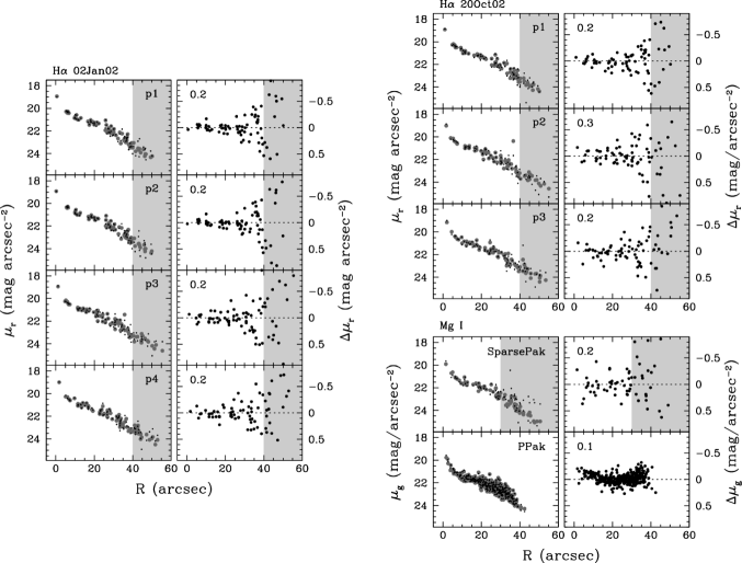
Figure 19.— Photometric calibration of the IFS fiber continuum flux. Three panel groups are shown: the results for the four H$\alpha$ 02Jan02 SparsePak pointings, the results for the three H$\alpha$ 20Oct02 pointings, and the results for the two Mg i pointings — one from SparsePak and the other from PPak. Each group has two columns, overlaying the calibrated fiber fluxes (black) on the measured aperture photometry from the SDSS images (gray) to the left and plotting the residual, $\Delta\mu=\mu_{\rm fib}-\mu_{\rm CCD}$, to the right. Radial regions not considered during the calibration process are shaded gray. The pointing number or instrument is provide in the upper-right corner of the left-column panels, and the RMS of the residuals are displayed in the upper-left corner of the right-column panels.

The interpolation of the continuum fluxes and kinematics from our IFS is performed to fill interstitial fiber regions according to the following algorithm: Each kinematic measurement contributes to every pixel in the image, weighted by a two-dimensional Gaussian function centered on the fiber aperture with a FWHM equal to a multiple of the effective fiber diameter, $D_{\rm fib}$, and inversely weighted by the measurement error; therefore, each image pixel is weighted both by the quality and proximity of the surrounding fiber measurements. Mathematically, the weight of each fiber $f$ at pixel coordinate ($j$,$k$) is, therefore,

$$w_{f}(j,k)=\frac{1}{\epsilon_{f}^{2}}\exp\left[\frac{-(x_{j}-x_{f})^{2}-(y_{k}-y_{f})^{2}}{(nD_{\rm fib}/2)^{2}/\ln 2}\right],$$ (A2)

where $\epsilon_{f}$ is the measurement error, ($x_{j},y_{k}$) are the on-sky coordinates of pixel ($j$,$k$), the fiber center has on-sky coordinates ($x_{f},y_{f}$), and $nD_{\rm fib}$ is the FWHM of the circular Gaussian in multiples of the fiber diameter. Calibrated continuum fluxes include no additional error weighting ($\epsilon_{f}$ is constant for all $f$). The interpolated value at each pixel is then the weighted average, over all fibers, of the continuum value or kinematic measurement in question. For presentation purposes, we limit the interpolation to only those regions with a “significant” contribution to the interpolated map. For Figure 1, we adopt the following representation of “significant:”

$$\sum_{f=1}^{N_{f}}w_{f}(j,k)\geq\frac{w_{\rm min}}{N_{x}N_{y}}\sum_{j=0}^{N_{x}-1}\ \sum_{k=0}^{N_{y}-1}\ \sum_{f=1}^{N_{f}}w_{f}(j,k),$$ (A3)

where $N_{x}$ and $N_{y}$ are the pixel dimensions of the image. That is, the summed weight of all fibers to a given pixel must be greater than $w_{\rm min}$ times the mean of all weights across the entire image. This scheme is not ideal given the dependence between the inclusion of an interpolated value and the arbitrary size of the image; however, it can provide reasonable results as demonstrated by Figure 1. Values of $n$ and $w_{\rm min}$ for each of the 5 interpolated maps in Figure 1 are provided in Table 9.

Table 9Interpolation Parameters for Figure 1

Quantity	$n$	$w_{\rm min}$
$\mu_{{\rm H}\alpha}$	1.4	0.5
$V_{{\rm H}\alpha}$	1.4	0.1
$\mu_{\mbox{\scriptsize Mg{$~{}\!$i}}}$	1.2	0.5
$V_{\ast}$	1.8	0.1
$\sigma_{\ast}$	1.8	0.1

Appendix B Optimal Weighting Scheme for Kinematic Inclination Measurements

In velocity-field modeling, parameter robustness and covariance can be, respectively, improved and mitigated by introducing data-weighting schemes. For example, Begeman (1989) introduced a cosine weighting scheme, effectively weighting each datum by the derivative of the model LOS velocity with respect to the projected rotation velocity, $w=\partial V_{\rm LOS}/\partial V_{\rm rot}^{\rm proj}=\cos\theta$, thereby limiting the covariance between $V_{\rm rot}$ and $i$. Andersen & Bershady (2003) mitigate this same covariance by instead fitting the projected rotation curve directly. Here, we consider an optimal weighting scheme for measuring the kinematic inclination of UGC 463 according to the approach described in Section 3.1.1.

Andersen & Bershady (2003) parameterized $V_{\rm rot}^{\rm proj}(R)$ by a hyperbolic tangent function and adopted a velocity-error weighting scheme, producing a face-on TF relation that is well matched to samples of more inclined systems. Their error-weighting scheme combines, in quadrature, the measured velocity error with a “beam-smearing error” and a “stochastic error.” The beam-smearing error is based on a fiber-by-fiber measurement of the variance in $V_{\rm LOS}$ within the fiber aperture, thereby reducing the effect of patchy emission on the fit. The stochastic error is a single error assessed for every velocity measurement that reduces the influence of small-scale, incoherent non-circular motions on the fit.

Here, we are primarily concerned with fitting inclination such that we test the success/failure of a given weighting function, as applied to UGC 463, via the correspondence/disparity of the inclinations determined from each of three tracers: (1) H$\alpha$ from SparsePak, $i_{\mbox{\scriptsize H$\alpha$}}$; (2) [O iii] from PPak, $i_{\mbox{\scriptsize[O{$~{}\!$iii}]}}$; and (3) stars from PPak, $i_{\ast}$. We apply four weighting schemes: In addition to the error-based and $\cos\theta$ schemes described above, we include uniform weighting and a weighting scheme defined by $w=\partial V_{\rm LOS}/\partial i$. The latter scheme affords those data with greater leverage on the fitted inclination a greater influence on the goodness-of-fit statistic.

We omit data from consideration in our goodness-of-fit statistic in two steps. First, we omit all data with velocity errors that are greater than 15 km s^-1, eliminating 0.5%, 0%, and 1.0% of the SparsePak H$\alpha$, PPak [O iii], and PPak stellar data, respectively. We note here that, after applying this omission, the mean velocity measurement errors are 1, 3, and 6 km s^-1 for the SparsePak H$\alpha$, PPak [O iii], and PPak stellar data, respectively. Second, we omit highly discrepant velocities by first fitting the data using the error weighting scheme and omitting data at high $\chi^{2}$. Data are iteratively omitted while adjusting the model and the stochastic error until the error-weighted distribution of the data about the model follows a nominal Gaussian (Westfall, 2009); in practice, no points are omitted with $\chi^{2}=(V-V_{m})^{2}/\epsilon(V)^{2}<10$. This omission stategy does not bias our results toward, e.g., the initial guess parameters of the fit; instead, it serves to eliminate a $\chi^{2}$-optimization bias driven by a few, highly discrepant measurements. Applying this procedure to our UGC 463 data eliminates an additional 11.6%, 14.0%, and 5.2% of the SparsePak H$\alpha$, PPak [O iii], and PPak stellar data, respectively. As described in Section 3.1.1, all velocity-field parameters are simultaneously fit to the remaining data with the dynamical center of the PPak data fixed to the morphological center. Identical data sets are fit by each weighting scheme for each tracer, and we use a set of 500 bootstrap simulations (see Section 15.6.2 of Press et al., 2007) to determine the probability distribution for each fitted parameter. The error-weighted standard deviations of the velocities about the best-fitting models are typically 5, 6, and 7 km s^-1 for the SparsePak H$\alpha$, PPak [O iii], and PPak stellar data, respectively, with only small ($5-10$%) variations among results reached using the different weighting schemes.

Figure 20 provides the bootstrap-based probability distributions and growth curves for the inclinations measured by each weighting scheme and each tracer; the best-fit inclination and the 68% confidence limits are tabulated in the Figure. For UGC 463, we find that weighting by $\partial V_{\rm LOS}/\partial i$ produces inclination distributions that are the most similar between the three kinematic tracers. This is, therefore, the weighting scheme we have adopted in Section 3.1.1 to measure $i_{\rm kin}$. For all results except those based on the error-weighting scheme, the error-weighted mean of $i_{\mbox{\scriptsize H$\alpha$}}$, $i_{\mbox{\scriptsize[O{$~{}\!$iii}]}}$, and $i_{\ast}$ is compatible with our final adopted inclination of $i=27\arcdeg\pm 2\arcdeg$ to better than the errors.

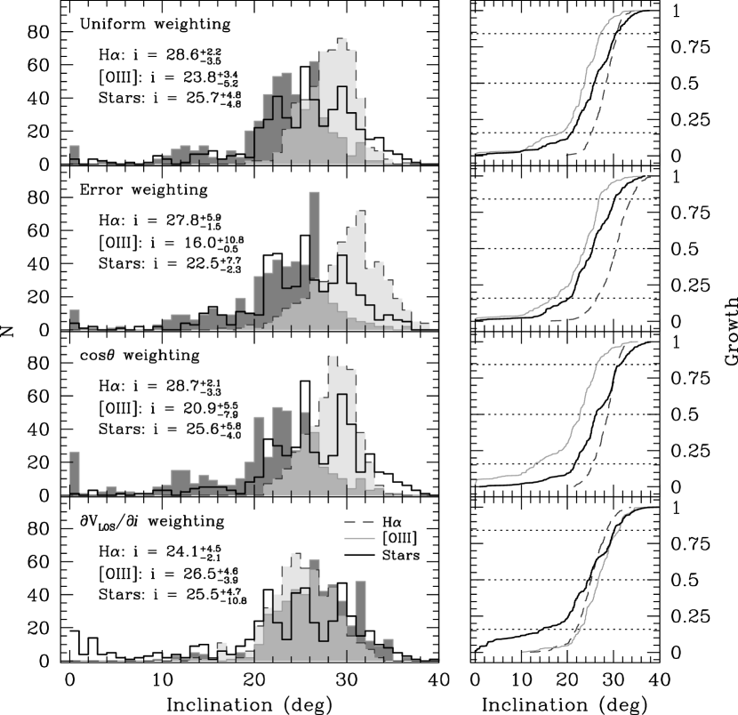
Figure 20.— Inclination probability distributions determined from 500 bootstrap simulations for each tracer using four different weighting schemes. Left — Histogram of the returned inclination values. The fitted inclination for each tracer is tabulated in the upper-left corner of each panel. The line key for each histogram is shown in the lower-left panel. The SparsePak H$\alpha$ histogram is shaded in light (transparent) gray and the PPak [O iii] histogram is shaded in dark gray. Right — Growth curves of each histogram from the left panels. The line types are repeated from the left column. The dotted lines mark the median (0.5 growth) and the 68% confidence interval ($0.16-0.84$ growth).

References

- Agertz et al. (2009) Agertz, O., Lake, G., Teyssier, R., Moore, B., Mayer, L., & Romeo, A. B. 2009, MNRAS, 392, 294
- Agertz et al. (2011) Agertz, O., Teyssier, R., & Moore, B. 2011, MNRAS, 410, 1391
- Amorisco & Bertin (2010) Amorisco, N. C., & Bertin, G. 2010, A&A, 519, 47