Spin Conduction in Anisotropic $3-D$ Topological Insulators

Abstract

When topological insulators possess rotational symmetry their spin lifetime is tied to the scattering time. We show that in anisotropic topological insulators this tie can be broken and the spin lifetime can be very large. Two different mechanisms can obtain spin conduction over long distances. The first is tuning the Hamiltonian to conserve a spin operator $\cos\phi\,\sigma_{x}+\sin\phi\,\sigma_{y}$, while the second is tuning the Fermi energy to be near a local extremum of the energy dispersion. Both mechanisms can produce persistent spin helices. We report spin lifetimes and spin diffusion equations.

I Introduction

Topological insulators Fu and Kane (2007); Zhang et al. (2009a); Hasan and Kane (2010); Liu et al. (2010a) exhibit a gap in the spectrum of bulk states, and bridging that gap is a band of surface states; if the Fermi energy is within the gap then electrons flow only along the surface and not in the bulk. At small enough momenta the surface band has the shape of two cones joined at their ends. One Dirac cone describes electrons with positive energies, and the other describes negative energies. An electron’s spin is locked to its momentum, so backscattering is suppressed. All these properties are consequences of time-reversal ($T$) symmetry, and are robust against small perturbations which are $T$-symmetric, such as non-magnetic impurities.

Recently much attention has been given to creating topologically protected qubits at the interface between a 3-D topological insulator (TI) and a conventional superconductor, allowing robust quantum arithmetic Fu and Kane (2008). The TI spin-momentum locking attracts attention to spintronics; recent works have shown that circularly polarized light could induce spin currents McIver et al. (2011) and topological phase transitions Inoue and Tanaka (2010).

This paper’s main focus is on obtaining good spin conductors suitable for spintronics. Disordered TIs are unusually poor spin conductors. Because electronic spin is tied to momentum, each scattering event randomizes the spin, as is typical of Elliot-Yafet spin relaxation Wenk et al. (2010). On the Dirac cone the spin lifetime $\tau_{s}$ is tightly coupled Burkov and Hawthorn (2010) to the scattering time $\tau$ by $\tau_{s}/\tau=2$. Ordinary semiconductors have much longer spin lifetimes, because spin is conserved during scattering and is randomized only by precession between scattering events. In this paper we will describe how to tune a TI for very long spin lifetimes ($\tau_{s}\gg\tau$), allowing spin to conduct over long distances.

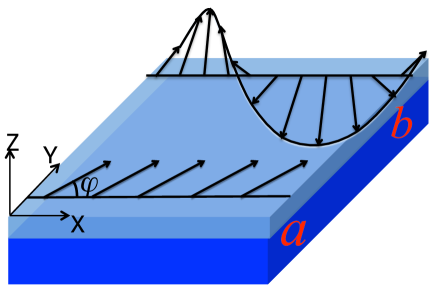
Figure 1: Two spin profiles that conduct in properly tuned TIs. The light blue and dark blue represent the conducting surface and the insulating bulk of a 3-D topological insulator. Line a shows a spatially uniform spin density. Line b shows a persistent spin helix which oscillates along the x axis and is spatially uniform along the y axis. The PSH is a standing wave; it does not precess.

We will show that the two spin profiles shown in Figure  1 conduct in a properly tuned TI. The first profile lies in the surface plane and its angle $\phi$ in that plane is constant. The spin component $S_{\phi}$ aligned with $\phi$ conducts: its integral $\int{d\vec{x}}\,S_{\phi},\,S_{\phi}\equiv\ cos\phi S_{x}+\sin\phi S_{y}$ is conserved ($\tau_{s}=\infty$) and its long-wavelength variations equilibrate diffusively, similarly to heat diffusion. Spin at right angles to the unit vector $\hat{e}_{\phi}$ is filtered out very quickly, relaxing with lifetime $\tau_{s}=\tau$. Figure  1b shows the second spin profile which conducts in a properly tuned TI: a standing spin wave which repeats at intervals of $\pi/|\hat{Q}|$. Because it rotates its spin orientation and does not decay, it is called a persistent spin helix (PSH) Bernevig et al. (2006). Associated with the PSH is a conserved quantity $\int{d\vec{x}}\,S_{PSH},\;S_{PSH}=\cos(2\hat{Q}\cdot\vec{x})(-\sin\phi S_{x}+\cos\phi S_{y})+\sin(2\hat{Q}\cdot\vec{x})S_{z}$. If $\phi=0$ the PSH rotates in the $y-z$ plane, while if $\phi=\pi/2$ it rotates in the $x-z$ plane. The spin orientation $\phi$, the wave-vector $2\hat{Q}$, and the diffusion constant all depend on the details of the TI Hamiltonian.

Tuning for spin conduction is not possible unless the surface band is more complex than a simple Dirac cone. Anisotropy, i.e. violation of rotational invariance , is key to long distance spin conduction. This is the origin of the spin orientation angle $\phi$ which parameterizes both spin profiles. Anisotropy can be realized in TIs either by choosing reduced-symmetry materials like $\beta-Ag_{2}Te$ Zhang et al. (2011); Virot et al. (2011) (see Figure  2b) or by cutting a high-symmetry TI in a way that reduces the surface’s symmetry Egger et al. (2010); Moon et al. (2011). Figure  2 illustrates distortion of the Dirac cone as rotational symmetry is progressively broken. We use simple linear models that are appropriate near the Dirac point. Figure  2a shows the dispersion of a rotationally symmetric system. Figure  2b shows the Dirac cone stretching along one axis as rotational symmetry is broken. Finally Figure  2c extrapolates the stretching to its extreme: the energy dispersion depends only on $k_{x}$ not $k_{y}$, and therefore an operator $\cos\phi\,\sigma_{x}+\sin\phi\,\sigma_{y}$ is necessarily conserved.

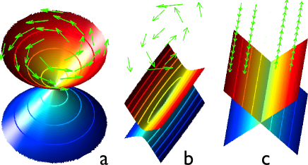
Figure 2: Anisotropy in TIs. (a - isotropic) the Rashba Hamiltonian $H_{R}=\hbar v_{F}(k_{y}\sigma_{x}-k_{x}\sigma_{y})$, (b - stretched) linear terms from a $k\cdot p$ model of $\beta-Ag_{2}Te$, (c - infinitely stretched) a tuned model $H_{1}=\hbar v_{F}k_{x}(\cos\phi\,\sigma_{x}+\sin\phi\,\sigma_{y})$ which conserves the spin operator $\cos\phi\,\sigma_{x}+\sin\phi\,\sigma_{y}$. The colored surfaces show the energy dispersion $E(\vec{k})$, and the lines inscribed on them show Fermi surfaces - contours of constant energy. The arrows show the spin orientation, which is locked to the momentum.

There are two ways to tune for spin conduction. The first is to tune the Hamiltonian for conservation of a spin operator $\cos\phi\sigma_{x}+\sin\phi\sigma_{y}$, causing $S_{\phi}$ to conduct. This has been achieved in GaAs quantum wells by tuning both the well width and the well depth to obtain partial cancellation of the Rashba and Dresselhaus terms Schliemann et al. (2003); Bernevig et al. (2006); Koralek et al. (2009). These tuned quantum wells are modeled by a Hamiltonian that includes both a spin-conserving quadratic term $\frac{\hbar^{2}|\vec{k}|^{2}}{2m}$ and a small linear spin-orbit term which conserves $\cos\phi\sigma_{x}+\sin\phi\sigma_{y}$, as illustrated in Figure  3c. They manifest a PSH-induced strong enhancement of the spin lifetime. The TI model of Figure  2c also conducts both $S_{\phi}$ and PSH’s with wave-vector $\pm 2\hat{Q}=\pm 2\frac{E_{F}}{v_{F}}\hat{x}$.

We will show that there is a second way to obtain spin conduction if the surface band has local extrema at $\vec{k}=\pm\hat{Q}\neq 0$, in which case tuning the Fermi energy near the energy $E_{Q}$ of the extrema will produce very long spin lifetimes. Figure  3 shows that even a small anisotropy will produce the required local minima. The model shown in Figure  3a includes a quadratic term and a spin-orbit term, both of which are rotationally symmetric. It shows four Fermi surfaces - contours of constant energy. Two Fermi surfaces are at $E_{F}=-0.163$, two are at $E_{F}=-0.24$, and all four are perfect circles. The minimum of the energy dispersion is also a circle located midway between the dotted $E_{F}=-0.24$ Fermi surfaces. In Figure  3b the rotational symmetry is only slightly broken - the spin-orbit term’s strength is only $20\%$ smaller along the $x$ axis than it is along the $y$ axis. Nonetheless the Fermi surfaces have already divided and wrapped themselves around the dispersion’s local minima which are now two discrete points located inside the dotted $E_{F}=-0.24$ Fermi surfaces. Model  3b does not conserve any spin operator, but we will show that it conducts spin when $E_{F}$ is adjusted so that the Fermi surfaces lie close to the the local minima. Lastly Figure  3c reduces the spin-orbit term along the $x$ axis to zero, and exhibits spin conduction at any value of $E_{F}$. In both Figures  3b and  3c spin conduction is associated with there being two disconnected Fermi surfaces centered on the local extrema. Spin conduction in TI’s is possible only when anisotropy changes the global structure of the Fermi surface.

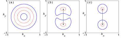
Figure 3: Fermi surfaces showing that anisotropy causes local extrema. $H=\frac{k^{2}}{2m}+v_{x}k_{x}\sigma_{y}+v_{y}k_{y}\sigma_{x},\,m=0.5,\,v_{y}=1$. The solid blue lines are Fermi surfaces at energy $E_{F}=-0.163$, while the dashed red lines are at $E_{F}=-0.24$. All quantities are unitless. (a) Isotropic $v_{x}=1$, (b) anisotropic $v_{x}=0.8$, (c) spin conserving $v_{x}=0$. (a) and (b) are typical of untuned spin-orbit couplings in quantum wells, while (c) is the same as Bernevig et al’s model Bernevig et al. (2006) of a tuned quantum well. The dashed Fermi surfaces in (b) and (c) lie near local minima. Model (b) conducts spin $S_{x}$ when $E_{F}\approx E_{Q}$, while (c) always conducts $S_{x}$. The arrows point out the Fermi surface nesting symmetry which causes PSH’s in both models.

In order to understand this global physics, we calculate charge and spin conduction for a very general class of $T$-conserving spin-orbit Hamiltonians: $H_{gen}=a_{x}(\vec{k})\sigma_{x}+a_{y}(\vec{k})\sigma_{y}+a_{I}(\vec{k})$, where $a_{x},a_{y}$ are odd in $\vec{k}$ and $a_{I}$ is even. This describes charge moving in the $x-y$ plane, on one surface of a 3-D TI . We study the single-particle density matrix $\rho=\psi^{\dagger}\psi$, which is a $2\times 2$ matrix in spin space. We write it as a $4-$vector $\vec{\rho}=\begin{bmatrix}N,&S_{x},&S_{y},&S_{z}\end{bmatrix}$ containing the charge density $N={Tr}(\rho)$ and spin densities $S_{x},S_{y},S_{z}={Tr}(\rho\sigma_{i})/2$. We will first analyze $\vec{\rho}$’s structure, and later calculate its diffusion induced by disorder.

II Spin Profiles

The spatially uniform and PSH profiles shown in Figure  1 manifest themselves in the Fourier-transformed density matrix $\rho(\vec{q})\propto\int{d\vec{k}}\,\psi^{\dagger}(\vec{q}/2+\vec{k})\psi(-\vec{q}/2+\vec{k})$ as strong peaks at $\vec{q}=0$ and at $\vec{q}=\pm 2\hat{Q}$. These peaks are directly linked to the TI Fermi surface: the state vector $\psi$ is populated only by states from the Fermi surface, and therefore $\rho(\vec{q})$ is peaked when $\vec{q}$ maximizes the intersection of the Fermi surface with a copy of itself shifted by $\vec{q}$. (The dominance of the Fermi surface is assured if $E_{F}\tau/\hbar\gg 1$, the temperature is small, and there are no interactions.) The spatially uniform peak $\rho(\vec{q}=0)$ realizes this maximization trivially.

Figures  3b and  3c illustrate a special nesting symmetry which produces PSH peaks at $\vec{q}=\pm 2\hat{Q}$. They show pairs of Fermi surfaces centered at $\pm\hat{Q}$ which possess inversion symmetry ($\hat{Q}\rightarrow-\hat{Q}$) because of the TI’s $T$ symmetry. The Fermi surfaces also possess nesting symmetry, which means that a shift of $\vec{q}=\pm 2\hat{Q}$ moves one Fermi surface on top of the other. This nesting symmetry produces peaks in $\rho(\vec{q})$ at $\vec{q}=\pm 2\hat{Q}$; it is responsible for PSH’s. The nesting symmetry can be written as $\hat{Q}+\vec{k}\rightarrow-\hat{Q}+\vec{k}$, where $\hat{Q}+\vec{k}$ lies on one Fermi surface and $-\hat{Q}+\vec{k}$ lies on the other one. $T$ plus nesting implies that the Fermi surface near $\hat{Q}$ possesses inversion symmetry around $\hat{Q}$: $\hat{Q}+\vec{k}\rightarrow\hat{Q}-\vec{k}$.

The TI surface has only one conduction band and only one valence band, with spin quantum number equal to $s=+1,-1$ respectively. We assume that the Fermi surface lies only in the conduction band; $s=+1$. As a result the spatially uniform $S_{z}$ spin density is identically zero: $S_{z}(\vec{q}=0)$’s contributing terms are of the form $S_{z}\propto{Tr}(\rho_{k}\sigma_{z})/2,\,\rho_{k}=\psi^{\dagger}(\vec{k})\psi(\vec{k})$, which is zero for all $\psi$ in the conduction band. Similarly the charge $N(\vec{q}=2\hat{Q})$ and spin $S_{\phi}(\vec{q}=2\hat{Q})$ components of the PSH are zero, because $\rho(2\hat{Q})\propto\psi^{\dagger}(\vec{Q})\psi(-\vec{Q})$ and $T$ symmetry ensures that $N(2\hat{Q})={Tr}(\rho(2\hat{Q}))$ and $S_{\phi}={Tr}(\rho(2\hat{Q})\,(\cos\phi\,\sigma_{x}+\sin\phi\,\sigma_{y})/2)$ are zero when $\psi$ is in the conduction band.

III Diffusive Conduction

Figure 4: Diffusion diagram with two joint scatterings. A single joint scattering event $I_{ij}$ corresponds to a pair of Green’s functions $G^{A}$ and $G^{R}$ connected by a dashed line. The dotted legs correspond to the external propagators.

We now consider adding a non-magnetic ”white noise” disorder potential $V$ to the general Hamiltonian $H_{gen}$, where $V=\begin{bmatrix}1&0\\ 0&1\end{bmatrix}u(\vec{r}),\,\langle u(\vec{r})u(\acute{\vec{r}})\rangle=n_{i}u_{0}^{2}\delta(\vec{r}-\acute{\vec{r}})$, and $n_{i}u_{0}^{2}$ gives the disorder concentration and strength. When disorder is present the density matrix evolves diffusively at time scales larger than the elastic scattering time. Its evolution is controlled by the partial differential equation $\mathcal{D}_{ij}^{-1}\vec{\rho}=0$, where the $4\times 4$ matrix $\mathcal{D}_{ij}$ is called the diffuson. The diffuson’s matrix structure couples the charge and spin densities to each other. We derive the diffuson using standard methods from the diagrammatic technique for disordered systems Hikami et al. (1980); Suzuura and Ando (2006); McCann et al. (2006), couched in the notation of References Burkov et al., 2004; Burkov and Hawthorn, 2010. Within this diagrammatic technique the conductivity is determined by the disorder-averaged two-particle correlation function, which is controlled by ladder diagrams at leading order in $(E_{F}\tau/\hbar)^{-1}$. The diffuson is composed of an infinite series of ladder diagrams like that seen in Figure  4. These diagrams describe sequences of events in which $\psi$ and $\psi^{\dagger}$ move together, scattering in unison. A single joint scattering event is described by the operator $I_{ij}$, and the diffuson sums diagrams with any number of joint scatterings; $\mathcal{D}_{ij}(\vec{q},\omega)=\sum_{n=0}^{\infty}(I_{ij})^{n}=(1-I_{ij})^{-1}$. The joint scattering operator $I_{ij}$ is pictured in Figure  4 and is given by the integral

$$\begin{split}I_{ij}=\frac{n_{i}u_{0}^{2}}{2}\int d\vec{k}\,{Tr}(\,G^{A}(\vec{k}-\vec{q}/2,E_{F})\\ \sigma_{i}\,G^{R}(\vec{k}+\vec{q}/2,E_{F}+\hbar\omega)\,\sigma_{j}\,)\end{split}$$ (1)

$G^{A}$ and $G^{R}$ are the disorder-averaged single-particle Green’s functions which express uncorrelated movements of $\psi$ and $\psi^{\dagger}$, while $\vec{q}$ is the diffuson momentum. The trace is taken over the spin indices of $G^{A},G^{R},\sigma_{i},$ and $\sigma_{j}$, which are all $2\times 2$ matrices in spin space.

The zero-frequency component of the diffuson $\mathcal{D}_{ij}(\vec{q}=0,\omega=0)$ is equal to $\hat{\tau}_{s}/\tau$, where $\hat{\tau}_{s}$ is the tensor that governs relaxation of spatially uniform spin profiles. Assuming as before that the Fermi surface is dominant ($E\tau/\hbar\gg 1$) and contains only the conduction band, we find:

$$\hat{\tau}_{s}/\tau=2\begin{bmatrix}0&0&0\\ 0&(1-\langle\cos 2\theta\rangle_{F})&-\langle\sin 2\theta\rangle_{F}\\ 0&-\langle\sin 2\theta\rangle_{F}&(1+\langle\cos 2\theta\rangle_{F})\end{bmatrix}^{-1}$$ (2)

This result is fully general for all $H_{gen}$. The angle $\theta(\vec{k})$ gives the relative strength of the $a_{x}\sigma_{x}$ and $a_{y}\sigma_{y}$ terms, and is defined by $\tan\theta=a_{y}/a_{x}$. The average $\langle\;\rangle_{F}$ is over the entire Fermi surface(s), and is weighted by the density of states. The zeros mean that the charge lifetime is infinite; charge is conserved. Linear combinations of $S_{x},S_{y}$ have lifetimes $2\tau/(1\pm\sqrt{\langle\cos 2\theta\rangle_{F}^{2}+\langle\sin 2\theta\rangle_{F}^{2}})$; spin conduction is obtained only if

$$1={\langle\cos 2\theta\rangle_{F}^{2}+\langle\sin 2\theta\rangle_{F}^{2}}\,.$$ (3)

Equation 3 confirms our earlier statement that spin conduction can be obtained by tuning for conservation of a spin operator $\cos\phi\,\sigma_{x}+\sin\phi\,\sigma_{y}$. In this case $|\cos\theta|,\,|\sin\theta|$ are equal to the constants $|\cos\phi|,\,|\sin\phi|$ and equation 3 is trivially satisfied. Figure  5 shows the spectrum of the inverse diffuson in two models which conserve $\cos\phi\,\sigma_{x}+\sin\phi\,\sigma_{y}$. Both models have two null eigenvalues at $q_{x}=0$, corresponding to conduction of charge and of $S_{\phi}$. Both models also exhibit a single null eigenvalue at $q_{x}=\pm 2\hat{Q}$, implying PSH conduction. Models which both conserve $\cos\phi\,\sigma_{x}+\sin\phi\,\sigma_{y}$ and have a nesting symmetry with $\theta(\hat{Q})=\phi$ always exhibit PSH’s. When the nesting symmetry is only approximate, the PSH lifetime is ${\tau_{PSH}}=\hbar^{2}/(4\tau\langle(\delta E)^{2}\rangle_{F}),\,\delta E=\vec{\xi}\cdot\nabla_{k}E(\hat{Q})$. The gradient in this formula measures violation of the inversion symmetry $\hat{Q}+\vec{k}\rightarrow\hat{Q}-\vec{k}$. $\vec{\xi}=\vec{k}-\hat{Q}$ is the displacement of the Fermi surface from the extremum.

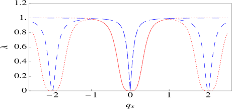
Figure 5: Smallest two eigenvalues (absolute values) of the inverse diffuson as a function of momentum. Zeros occur both at $\vec{q}=0$ and at $\vec{q}=\pm 2\hat{Q}$, implying conduction of both the spatially uniform spin profile and PSH’s. Dashes and dots are for the linear and quadratic models seen in Figures  2c and  3c respectively. The Fermi energy $E_{F}$ has been tuned to match the local minima seen in Figure  3c. The momentum scale is $\hat{Q}=|\hat{Q}|\hat{x}$, and $\tau\,E_{F}=8$.

Equation 3 also confirms that tuning the Fermi energy can produce spin conduction. The key is that this equation concerns only the Fermi surface: $|\cos\theta|$ and $|\sin\theta|$ must be constant there. When $E_{F}$ is tuned close to a local extremum the Fermi surface becomes very small. Therefore $|\cos\theta|,\,|\sin\theta|$ are nearly constant on the Fermi surface, $\cos\phi\,\sigma_{x}+\sin\phi\,\sigma_{y},\,\phi=\theta(\hat{Q})$ is nearly conserved there, and $S_{\phi}$ conducts freely.

Tuning the Fermi energy also can produce PSH’s. $T$ symmetry requires that extrema always come in pairs at $\vec{k}=\pm\hat{Q}$. The Fermi surfaces $\mathcal{S}_{\pm}$ accompanying these pairs possess the nesting symmetry which produces PSH’s. However there must be no scattering between the pair of Fermi surfaces $\mathcal{S}_{\pm}$ and any other Fermi surfaces, because $\cos\phi\,\sigma_{x}+\sin\phi\,\sigma_{y},\,\phi=\theta(\hat{Q})$ will not be conserved on the other surfaces. If there are additional Fermi surfaces then the disorder potential must be smooth, without short-wavelength variations. In this case there will be one pair of persistent spin helices for each pair of extrema.

We have computed the spin lifetime when there are local extrema. For the spatially uniform spin profile it is $\tau_{s}/\tau=1/\langle(\delta\theta)^{2}\rangle_{F},\,\delta\theta=\vec{\xi}\cdot\nabla_{k}\theta(\hat{Q})$. The PSH lifetime is double this value. Our PSH calculation is valid only in the diffusive regime where the PSH characteristic length $l_{PSH}=h/2|\hat{Q}|$ is large compared to the scattering length $l_{\tau}$. $\delta\theta$ measures the amount that $\theta$ varies on the Fermi surface, because when $\theta$ is constant $S_{\phi}$ is conserved and $\tau_{s}=\infty$. $\vec{\xi}$ measures the width of the Fermi surface; when $E_{F}$ approaches the extremum it goes to zero and the spin lifetime diverges. For instance, in the quadratic model $H=\frac{k^{2}}{2m}+v_{x}k_{x}\sigma_{y}+v_{y}k_{y}\sigma_{x},\,v_{y}>v_{x}$ shown in Figure  3 the lifetime is $\tau_{s}=\tau\frac{2mv_{y}^{2}(v_{y}^{2}-v_{x}^{2})}{v_{x}^{2}(E_{F}-E_{Q})}$. It diverges when spin is conserved ($v_{x}=0$) and also when the Fermi energy $E_{F}$ is tuned to the extremum $E_{Q}$. When the model is tuned for rotational symmetry $v_{x}\rightarrow v_{y}$ the lifetime becomes very small because the local minimum becomes very shallow, the Fermi surface stretches along the $x$ axis, and $\langle\xi_{x}^{2}\rangle_{F}\propto(E_{F}-E_{Q})/(v_{y}^{2}-v_{x}^{2})$ becomes very large.

Local extrema have already been realized in a TI Hsieh et al. (2008); Zhang et al. (2009b): $Bi_{1-x}Sb_{x}$, which has six fold symmetry. ARPES measurements Hsieh et al. (2008) reveal at least three six-fold degenerate minima, with momenta at $|\hat{Q}|\approx 0.15,0.8,1.1\text{\AA}^{-1}$. However the symmetry is too high: substitutional disorder causes scattering between all six minima. Moreover the bulk gap is very small, and the PSH length scale is so short that it may lie in the ballistic regime.

Local extrema will be found whenever there is an avoided band crossing in an anisotropic material. In $Bi_{1-x}Sb_{x}$ a conventional surface band occurs very close to the TI band. Repulsion between these two bands causes the observed local minima. Avoided band crossings have also been observed in very thin TI films - the TI bands on each of the film’s two surfaces couple to each other, causing band repulsion and extrema Lu et al. (2010); Linder et al. (2009); Liu et al. (2010b). The remaining necessary ingredient for spin conduction is anisotropy. In this respect the recent predictions of 10 to 1 anisotropy Zhang et al. (2011) in $\beta-Ag_{2}Te$ and 18 to 1 anisotropy in metacinnabar Virot et al. (2011) are very encouraging.

When spin conducts - for instance when $E_{F}$ is tuned near an extremum - the magnetoresistance will become null or even change sign. If only the spatially uniform profile conducts then there will be neither weak localization nor antilocalization (null magnetoresistance). If there are PSH’s then there will be a complete reversal from weak antilocalization to weak localization, from positive to negative magnetoresistance.

Returning to equation 1, we have calculated the diffuson operator $\mathcal{D}_{ij}$ which controls spin diffusion via $\mathcal{D}_{ij}^{-1}\vec{S}=0$. Our calculation is general for all $H_{gen}$ but considers only long wavelengths; i.e. momenta near $\vec{q}=0$. For brevity we will present here only the result when $\cos\phi\,\sigma_{x}+\sin\phi\,\sigma_{y}$ is conserved. The spin component orthogonal to $\hat{e}_{\phi}$ decays with lifetime $\tau_{s}=\tau$, and we have already seen that $S_{z}=0$. The spin diffusion equation for $N$ and $S_{\phi}$ is:

$$\begin{bmatrix}\partial_{t}-\frac{1}{2}\nabla_{x}\cdot D\cdot\nabla_{x}&-2\nabla_{x}\cdot\vec{\Gamma}\\ -\frac{1}{2}\nabla_{x}\cdot\vec{\Gamma}&\partial_{t}-\nabla_{x}\cdot D\cdot\nabla_{x}\end{bmatrix}\begin{bmatrix}N\\ S_{\phi}\end{bmatrix}=0$$ (4)

$$\vec{\Gamma} =\frac{1}{\hbar}\langle\nabla_{k}E(\vec{k})\rangle_{F},\;D=\frac{\tau}{\hbar^{2}}\langle\nabla_{k}E(\vec{k})\otimes\nabla_{k}E(\vec{k})\rangle_{F}$$

The charge-spin coupling $\nabla_{x}\cdot\vec{\Gamma}$ and the diffusion tensor $D$ are determined entirely by the energy dispersion. If the Fermi surface is an ellipse with height $h$ and width $w$ then $\vec{\Gamma}=0$ and $D=8\tau(E_{F}-E_{Q})^{2}/\hbar^{2}\,(w^{-2}\hat{x}\otimes\hat{x}+h^{-2}\hat{y}\otimes\hat{y})$. Assuming that the PSH length scale $l_{PSH}=h/2|\hat{Q}|\gg l_{\tau}$ is in the diffusive regime, we have derived the PSH diffusion equation:

$$(\partial_{t}+1/\tau_{PSH}-(\nabla_{x}-2\imath\hat{Q})\cdot D\cdot(\nabla_{x}-2\imath\hat{Q}))S_{PSH}=0$$ (5)

The term with two $(\nabla_{x}-2\imath\hat{Q})$ derivatives implies that small deviations from the spin helix relax diffusively.

IV Conclusion

In this article we studied spin conduction in a very general model of TI surfaces with non-magnetic disorder. We calculated the spin decay times and spin diffusion equations and found two ways to tune for a long spin lifetime and spin conduction. The first tuning mechanism is well known from quantum wells but new to TIs: tuning the Hamiltonian to conserve a spin operator. We found a second tuning mechanism: tuning the Fermi energy near a local extremum of the energy dispersion. Neither mechanism is possible unless the TI surface is anisotropic. Both mechanisms cause conduction of a spatially uniform spin profile. If the Fermi surfaces exhibit an additional nesting symmetry then Persistent Spin Helices will also conduct. When spin conduction is realized the TI’s magnetoresistance will be either null or negative, unlike an untuned TI where the magnetoresistance is positive. TIs which combine anisotropy with avoided band crossings will be promising candidates for spin conduction and PSH’s.

We acknowledge support from the NSF of China (Grant No. NSFC 10876042 and No. NSFC 10874158), the 973 program of China (Grant No. 2007CB925000 and No. 2011CBA00108)), and the WCU (World Class University) program of POSTECH through R31-2008-000-10059-0, Division of Advanced Materials Science. V. E. S. acknowledges the hospitality of AMS, POSTECH.

References

- Fu and Kane (2007) L. Fu and C. L. Kane, Physical Review B 76, 045302 (2007).
- Zhang et al. (2009a) H. Zhang, C.-X. Lu, X.-L. Qi, X. Dai, Z. Fang, and S.-C. Zhang, Nature Physics 5, 438 (2009a).
- Hasan and Kane (2010) M. Z. Hasan and C. L. Kane, Reviews in Modern Physics 82, 3045 (2010).
- Liu et al. (2010a) C.-X. Liu, X.-L. Qi, H. J. Zhang, X. Dai, Z. Fang, and S.-C. Zhang, Physical Review B 82, 045122 (2010a).
- Fu and Kane (2008) L. Fu and C. L. Kane, Physical Review Letters 100, 096407 (2008).
- McIver et al. (2011) J. W. McIver, D. Hsieh, H. Steinberg, P. Jarillo-Herrero, and N. Gedik, Nature Nanotechnology 7, 96 (2011).
- Inoue and Tanaka (2010) J. I. Inoue and A. Tanaka, Physical Review Letters 105, 017401 (2010).
- Wenk et al. (2010) P. Wenk, M. Yamamoto, J.-i. Ohe, T. Ohtsuki, B. Kramer, and S. Kettemann, in Quantum Materials, Lateral Semiconductor Nanostructures, Hybrid Systems and Nanocrystals, edited by D. Heitmann (Springer Berlin Heidelberg, 2010), NanoScience and Technology, pp. 277–302, URL http://dx.doi.org/10.1007/978-3-642-10553-1_11.
- Burkov and Hawthorn (2010) A. A. Burkov and D. G. Hawthorn, Physics Review Letters 105, 066802 (2010).
- Bernevig et al. (2006) B. A. Bernevig, J. Orenstein, and S.-C. Zhang, Physical Review Letters 97, 236601 (2006).
- Zhang et al. (2011) W. Zhang, R. Yu, W. Feng, Y. Yao, H. Weng, X. Dai, and Z. Fang, Physical Review Letters 106, 156808 (2011).
- Virot et al. (2011) F. Virot, R. Hayn, M. Richter, and J. van den Brink, Physical Review Letters 106, 236806 (2011).
- Egger et al. (2010) R. Egger, A. Zazunov, and A. L. Yeyati, Physics Review Letters 105, 136403 (2010).
- Moon et al. (2011) C.-Y. Moon, J. Han, H. Lee, and H. J. Choi, Physical Review B 84, 195425 (2011).
- Schliemann et al. (2003) J. Schliemann, J. C. Egues, and D. Loss, Physical Review Letters 90, 146801 (2003).
- Koralek et al. (2009) J. D. Koralek, C. P. Weber, J. Orenstein, B. A. Bernevig, S.-C. Zhang, S. Mack, and D. D. Awshalom, Nature 458, 610 (2009).
- Hikami et al. (1980) S. Hikami, A. I. Larkin, and Y. Nagaoka, Prog. Theor. Phys. Progress Letters 63, 707 (1980).
- Suzuura and Ando (2006) H. Suzuura and T. Ando, Journal of the Physical Society of Japan 75, 024703 (2006).
- McCann et al. (2006) E. McCann, K. Kechedzhi, V. I. Fal’ko, H. Suzuura, T. Ando, and B. L. Altshuler, Physical Review Letters 97, 146805 (2006).
- Burkov et al. (2004) A. A. Burkov, A. S. Nunez, and A. H. MacDonald, Physical Review B 70, 155308 (2004).
- Hsieh et al. (2008) D. Hsieh, D. Qian, L. Wray, Y. Xia, Y. S. Hor, R. J. Cava, and M. Z. Hasan, Nature 452, 970 (2008).
- Zhang et al. (2009b) H.-J. Zhang, C.-X. Liu, X.-L. Qi, X.-Y. Deng, X. Dai, S.-C. Zhang, and Z. Fang, Physical Review B 80, 085307 (2009b).
- Lu et al. (2010) H.-Z. Lu, W.-Y. Shan, W. Yao, Q. Niu, and S.-Q. Shen, Physical Review B 81, 115407 (2010).
- Linder et al. (2009) J. Linder, T. Yokoyama, and A. Sudbo, Physical Review B 80, 205401 (2009).
- Liu et al. (2010b) C.-X. Liu, H. J. Zhang, B. Yan, X.-L. Qi, T. Frauenheim, X. Dai, Z. Fang, and S.-C. Zhang, Physical Review B 81, 041307 (2010b).
- Oguchi and Shishidou (2009) T. Oguchi and T. Shishidou, Journal of Physics: Condensed Matter 21, 092001 (2009).