A superconvergent representation of the Gersten-Nitzan and Ford-Webber nonradiative rates

abstract

An alternative representation of the quasistatic nonradiative rates of Gersten and Nitzan [J. Chem. Phys. 1981, 75, 1139] and Ford and Weber [Phys. Rep. 1984, 113, 195] is derived for the respective parallel and perpendicular dipole orientations. Given the distance $d$ of a dipole from a sphere surface of radius $a$, the representations comprise four elementary analytic functions and a modified multipole series taking into account residual multipole contributions. The analytic functions could be arranged hierarchically according to decreasing singularity at the short distance limit $d\rightarrow 0$, ranging from $d^{-3}$ over $d^{-1}$ to $\ln(d/a)$. The alternative representations exhibit drastically improved convergence properties. On keeping mere residual dipole contribution of the modified multipole series, the representations agree with the converged rates on at least $99.9\%$ for all distances, arbitrary particle sizes and emission wavelengths, and for a broad range of dielectric constants. The analytic terms of the representations reveal a complex distance dependence and could be used to interpolate between the familiar $d^{-3}$ short-distance and $d^{-6}$ long-distance behaviors with an unprecedented accuracy. Therefore, the representations could be especially useful for the qualitative and quantitative understanding of the distance behavior of nonradiative rates of fluorophores and semiconductor quantum dots involving nanometal surface energy transfer in the presence of metallic nanoparticles or nanoantennas. As a byproduct, a complete short-distance asymptotic of the quasistatic nonradiative rates is derived. The above results for the nonradiative rates translate straightforwardly to the so-called image enhancement factors $\Delta$, which are of relevance for the surface-enhanced Raman scattering.

1 Introduction

The distance dependence of the nonradiative rate of a fluorophore or a semiconductor quantum dot relative to a metallic nanoparticle (MNP), or a nanoantenna, is of crucial importance for a number of novel techniques and nanodevices combining biomolecules, quantum dots, and MNP [1, 2, 3, 4, 5, 6, 7, 8, 9]. The MNPs can quench fluorescence as much as $100$ times better than other quenchers of fluorescence, such as DABCYL, and open new perspectives in the use of hybrid materials as sensitive probes in fluorescence-based detection assays [1]. In the case of single-stranded (ss) DNA probes labeled with a thiol at one end and a dye at the other, the ssDNA molecules self-organize into a constrained conformation on the MNP surface and the fluorophore is completely quenched by the particle through a distance-dependent process. Upon target (complementary oligo) binding, the constrained DNA conformation is opened because of a dramatic increase in the DNA rigidity that becomes double-stranded after hybridization. Thereby the fluorophore is separated from the particle surface, and the fluorescence of the hybrid molecule can increase by a factor of as much as several thousand as it binds to a complementary ssDNA [1]. This structural change generates a fluorescence signal that is highly sensitive and specific to the target DNA [1, 2], resulting in a molecular beacon that can detect minute amounts of oligonucleotide target sequences in a pool of random sequences and provide an improved detection of a single mismatch in a competitive hybridization assay for DNA mismatch detection [1]. MNP acceptors can also be employed for probing changes in distances for protein interactions on DNA using a molecular ruler approach involving nanometal surface energy transfer (NSET) from optically excited organic fluorophores to small MNPs [5, 6]. Whereas the traditional Förster resonance energy transfer (FRET) involving molecular acceptors and donors is efficient for the acceptor-donor separations up to $100$ Å, the use of MNP acceptors could more than double the traditional Förster range up to $220$ Å  [5, 6]. As it becomes apparent below, the reason for the extension of the traditional Förster range is a relaxed distance dependence relative to FRET, because the particle-fluorophore interaction could no longer be described by sole dipole-dipole interaction.

The nonradiative rates are derived from the total Ohmic loss, or the Joule heating, which is in general determined as the power $P_{abs}$ absorbed inside the particle [10, 11, 12, 13, 14, 15, 16, 17]

$$P_{abs}=\int_{V}Q({\bf r})\,d{\bf r}$$ (1)

where the volume integral extends over entire absorbing region. The quantity $Q$ is the steady (averaged) inflow of energy $Q$ per unit time and unit volume from the external sources which maintain the field, and which in the gauss units is given by

$$Q=\frac{ck_{0}}{8\pi}\left(\varepsilon^{\prime\prime}|{\bf E}|^{2}+\mu^{\prime\prime}|{\bf H}|^{2}\right)$$ (2)

where $k_{0}$ is the vacuum wave vector and $\varepsilon^{\prime\prime}$ ($\mu^{\prime\prime}$) is the imaginary part of the dielectric function (magnetic permeability) at the observation point. Alternatively, in the special case of an oscillating dipole source ${\bf p}e^{-i\omega t}$, one could consider the dipole moving in a local field produced by its surface image and calculate the dipole dissipated power by (see eq 3.1 of ref [13])

$$P_{abs}=\frac{\omega}{2}\,\mbox{Im }({\bf p}^{*}\cdot{\bf E}_{ind})$$ (3)

where ${\bf E}_{ind}e^{-i\omega t}$ is the electric field induced by the dipole at the dipole position ${\bf r}_{d}$, i.e. by the current source

$${\bf j}({\bf r},t)=-i\omega{\bf p}e^{-i\omega t}\delta({\bf r}-{\bf r}_{d})$$ (4)

The nonradiative rate $\Gamma_{nr}$ is then given by the correspondence principle

$$\Gamma_{nr}=\frac{P_{abs}}{\hbar\omega}$$ (5)

For the sake of definiteness, let the sphere center be located at the coordinate origin, the dipole position denoted be described by the position vector ${\bf r}_{d}$, $r_{d}=|{\bf r}_{d}|>a$ (see Figure 1), and the respective $\varepsilon$ and $\varepsilon_{0}$ be the sphere and host dielectric constants. Although exact expressions for the total, radiative, and nonradiative rates for a dipole interacting with a spherical particle [10, 11, 18, 19], including the case of a multi-coated sphere [14, 15], are known, and the F77 source codes could be freely downloaded [20], the quasi-static results of Gersten and Nitzan [12, 21] and Ford and Weber [13] (cf eqs 6 and 7 below) have nevertheless still retained their value. The quasi-static results for small enough sphere radius $a$ agree rather well with exact calculations [14, 16, 17] and experiment [7], and allow one for a valuable qualitative analytical insight. For a small separation $d$ of a fluorophore from a sphere surface, such that the dimensionless distance parameter $\delta=d/a\ll 1$, the quasi-static results predict a $d^{-3}$ dependence of the nonradiative rates (see eqs 32 and 33 below). The $d^{-3}$ short-distance dependence corresponds exactly to the case of a dipole located at the distance $d$ above a half-space characterized by the dielectric constant $\varepsilon$ [12, 13, 21]. However, as shown in Figures 4, 6 the $d^{-3}$ short-distance dependence begins to deviate rapidly from the converged rates for $\delta\gtrsim 0.1$ with increasing $\delta$. Thus, for a small MNP with $a\lesssim 10$ nm, the $d^{-3}$ short-distance dependence of the quasi-static nonradiative rates turns out to be valid only in an immediate proximity to the MNP ($d\lesssim 1$ nm) where the very use of the quasi-static rates is questionable. In the present work we remedy the above shortcomings by providing an analytic formula, which describes the distance behavior of the nonradiative rates over all distances with an unprecedented accuracy.

In what follows, we derive in Section 2 an alternative superconvergent representation of the quasistatic nonradiative rates (eqs 19, 24, 25 below) with drastically improved convergence properties. The superconvergent representation will be obtained by dividing the total contribution of each given multipole into a number of partial contributions (eqs 16, 22 below) so that the essential part of the partial contributions could be summed up analytically (eqs 17, 23 below) leaving behind a residual infinite multipole series. The first four exact sums are expressed in terms of elementary analytic functions of $u=(a/r_{d})^{2}$, with each subsequent function having a lesser singularity at the short distance limit $d\rightarrow 0$, ranging from $d^{-3}$ over $d^{-1}$ to $\ln(d/a)$. Convergence properties of the alternative representations are examined in Section 3. On keeping mere residual dipole term of the modified multipole series, the alternative representations are demonstrated to agree with the converged quasistatic nonradiative rates (eqs 6 and 7) of Gersten and Nitzan [12, 21] and Ford and Weber [13] on at least $99.95\%$ over entire length interval, for arbitrary particle sizes and emission wavelengths, and for a broad range of dielectric constants. In Section 4 the contribution of the analytic terms relative to that of the residual multipole series is analyzed. The alternative representations make it also possible to derive a complete short distance asymptotic of the classic quasi-static nonradiative rates including all singular terms in the distance parameter $\delta$. This is performed in Section 5. A two-term asymptotic will be shown to provide a significant improvement over the conventional $d^{-3}$ asymptotic over extended length scale. Keeping more terms in the asymptotic expansion improves the asymptotic in an immediate sphere proximity $\delta\ll 0.1$, but it comes at the expense of worsening the precision for $\delta\gtrsim 0.25$. In Section 6 common approaches for fitting experimental nonradiative rates are critically examined in light of the results of the present paper. In Section 7, the results for the nonradiative rates are shown to straightforwardly translate to the so-called image enhancement factors $\Delta$, which are of relevance for the surface-enhanced Raman scattering (SERS). The alternative superconvergent representations provide a significant improvement over the familiar $d^{-3}$ short-distance and $d^{-6}$ long-distance behaviors, and could be especially useful for the qualitative and quantitative understanding of the distance behavior of nonradiative rates of fluorophores and semiconductor quantum dots involving nanometal surface energy transfer in the presence of metallic nanoparticles or nanoantennas [1, 2, 3, 5, 6]. The remaining points are discussed in Section 8. We then conclude with Section 9.

2 Superconvergent representations of the quasistatic nonradiative rates

When calculating decay rates for a dipole interacting with a spherical particle, one distinguishes the cases of a perpendicular ($\perp$) and parallel ($\parallel$) dipole orientation relative to the sphere surface. The case of a general dipole orientation is then reduced to a linear combination of the two particular cases. Let $\bar{\varepsilon}=\varepsilon/\varepsilon_{0}$ be the relative dielectric constant, and let $\mu$ denote the molecular dipole. The nonradiative rates of Gersten and Nitzan [12, 21] for a perpendicular dipole orientation are (cf eq B.24’ of ref [21])

$$\Gamma_{nr}(\perp) = -\frac{|\mbox{\boldmath$\mu$}|^{2}}{2\hbar\varepsilon_{0}a^{3}}\sum_{l=1}^{\infty}(2l+1)\frac{(l+1)^{2}}{l}\left(\frac{a}{r_{d}}\right)^{2l+4}\mbox{Im }\frac{1}{\bar{\varepsilon}+\frac{l+1}{l}}$$ (6)

$$= \frac{|\mbox{\boldmath$\mu$}|^{2}}{2\hbar\varepsilon_{0}a^{3}}\sum_{l=1}^{\infty}(l+1)^{2}\left(\frac{a}{r_{d}}\right)^{2l+4}\mbox{Im }\frac{\bar{\varepsilon}-1}{\bar{\varepsilon}+\frac{l+1}{l}}$$

whereas the rates for a parallel dipole orientation are (see eq B.45’ of ref [21])

$$\Gamma_{nr}(\parallel) = -\frac{|\mbox{\boldmath$\mu$}|^{2}}{4\hbar\varepsilon_{0}a^{3}}\sum_{l=1}^{\infty}(l+1)(2l+1)\left(\frac{a}{r_{d}}\right)^{2l+4}\mbox{Im }\frac{1}{\bar{\varepsilon}+\frac{l+1}{l}}$$ (7)

$$= \frac{|\mbox{\boldmath$\mu$}|^{2}}{4\hbar\varepsilon_{0}a^{3}}\sum_{l=1}^{\infty}l(l+1)\left(\frac{a}{r_{d}}\right)^{2l+4}\mbox{Im }\frac{\bar{\varepsilon}-1}{\bar{\varepsilon}+\frac{l+1}{l}}$$

where Im denotes the imaginary part. The respective 2nd lines of eqs 6 and 7 have been obtained on using

$$\mbox{Im }\frac{1}{\bar{\varepsilon}+\frac{l+1}{l}}=-\frac{l}{2l+1}\,\mbox{Im }\frac{\bar{\varepsilon}-1}{\bar{\varepsilon}+\frac{l+1}{l}}$$ (8)

which follows from the identity:

$$\bar{\varepsilon}-1=\bar{\varepsilon}+\frac{l+1}{l}-\frac{2l+1}{l}$$ (9)

Occasionally, the Gersten and Nitzan [12, 21] expressions are written with an intrinsic molecular dipole moment $\mbox{\boldmath$\mu$}_{0}$ that is related to $\mu$ by (cf. eqs B.13, B.15 of ref [12])

$$\mbox{\boldmath$\mu$}=\mbox{\boldmath$\mu$}_{0}+\alpha E_{loc}=\frac{\mbox{\boldmath$\mu$}_{0}}{1-\Delta}$$ (10)

Here $E_{loc}$ is the local electric field that is in general affected by the presence of a sphere, $\alpha$ is the molecule polarizability, and $\Delta$ is a corresponding image enhancement factor. The intrinsic molecular dipole moment $\mbox{\boldmath$\mu$}_{0}$ is what would be found for a totally isolated molecule far away the sphere. $\Delta$ is significant only very close to the surface, in a region where the use of a classical approach and of the point dipole model for the molecule are questionable. Hence $\Delta$ may be disregarded in computing the actual decay rates [21]. The formulas (eqs 6 and 7) were independently confirmed by Ford and Weber, who determined the power dissipated by an arbitrary oriented dipole as (eq 3.47 of ref [13])

$$P_{abs}=\frac{\omega}{2\varepsilon_{0}a^{3}}\,\sum_{l=1}^{\infty}(l+1)\left[(l+1)\mbox{\boldmath$\mu$}_{\perp}^{2}+\frac{l}{2}\mbox{\boldmath$\mu$}_{\parallel}^{2}\right]\left(\frac{a}{r_{d}}\right)^{2l+4}\mbox{Im }\frac{l(\varepsilon-\varepsilon_{0})}{l\varepsilon+(l+1)\varepsilon_{0}}$$ (11)

where $\mbox{\boldmath$\mu$}_{\perp}$ and $\mbox{\boldmath$\mu$}_{\parallel}$ are the respective perpendicular and parallel components of $\mbox{\boldmath$\mu$}=\mbox{\boldmath$\mu$}_{\perp}+\mbox{\boldmath$\mu$}_{\parallel}$. When substituted in the correspondence principle (eq 5), the result for $P_{abs}$ leads to the nonradiative rates that are identical to those obtained by Gersten and Nitzan [12, 21].

In what follows, we employ a simple recipe to arrive at an alternative representation of the Gersten and Nitzan (GN) expressions (eqs 6 and 7) with drastically improved convergence properties. First note that the ‘Im’ sign in eqs 6 and 7 can be brought in front of the summation sign. Afterward, the task of deriving an alternative representation of the power series in eq 6 for a perpendicular dipole orientation reduces effectively to that for the power series

$$S_{\perp}=\sum_{l=1}^{\infty}(l+1)^{2}\frac{\bar{\varepsilon}-1}{\bar{\varepsilon}+1+\frac{1}{l}}\left(\frac{a}{r_{d}}\right)^{2l}=\frac{\bar{\varepsilon}-1}{\bar{\varepsilon}+1}\sum_{l=1}^{\infty}\frac{l(l+1)^{2}}{l+v}u^{l}$$ (12)

where $u$ and $v$ are the shorthands for

$$u=\left(\frac{a}{r_{d}}\right)^{2}, v=[\bar{\varepsilon}+1]^{-1}=\frac{\varepsilon_{0}}{\varepsilon+\varepsilon_{0}}$$ (13)

In terms of $S_{\perp}$,

$$\Gamma_{nr}(\perp)=\frac{|\mbox{\boldmath$\mu$}|^{2}}{2\hbar\varepsilon_{0}a^{3}}\,u^{2}\,\mbox{Im }S_{\perp}$$ (14)

Now follows a point of crucial importance. This is an iterative decomposition of the coefficients of the power series in eq 12 into decreasing powers of $l$. The iterative decomposition could be illustrated as follows. We begin to single out the leading $l^{2}$ dependence as follows

$$\frac{l(l+1)^{2}}{l+v}=\frac{(l+v-v)(l+1)^{2}}{l+v}=(l+1)^{2}-\frac{v(l+1)^{2}}{l+v}$$ (15)

Note that the last term in eq 15 is effectively of the order $l$ for $l\gg 1$, which is smaller than the $l^{2}$ order of the initial term. One can thus repeat the preceding step on the last term in eq 15, etc. By continuing the above iterative decomposition, one arrives at

$$\frac{l(l+1)^{2}}{l+v} = (l+1)^{2}-v(l+1)-v(1-v)-\frac{v(1-v)^{2}}{l}+\frac{v^{2}(1-v)^{2}}{l^{2}}-\frac{v^{3}(1-v)^{2}}{l^{2}(l+v)}$$ (16)

$$= l^{2}+l(2-v)+(1-v)^{2}-\frac{v(1-v)^{2}}{l}+\frac{v^{2}(1-v)^{2}}{l^{2}}-\frac{v^{3}(1-v)^{2}}{l^{2}(l+v)}$$

On applying the above decomposition in eq 12, the total contribution of each given multipole is divided into a number of partial contributions. The advantage of the decomposition is in that the first four partial contributions in eq. 16 could easily be summed up analytically. Indeed, upon substituting eq 16 back into eq 12, one obtains on using elementary summation formulas (eqs 46- 49 of Appendix A)

$$u^{2}S_{\perp}=\frac{\bar{\varepsilon}-1}{\bar{\varepsilon}+1}\,u^{2}\,\left[\frac{u(1+u)}{(1-u)^{3}}+\frac{u(2-v)}{(1-u)^{2}}\right.$$ (17)

$$\left.+\frac{u(1-v)^{2}}{1-u}+v(1-v)^{2}\,\ln(1-u)+v^{2}(1-v)^{2}\,F(u,v)\right]$$

where the remainder

$$F(u,v)=\sum_{l=1}^{\infty}\frac{u^{l}}{l(l+v)}=\sum_{l=1}^{\infty}\frac{u^{l}}{l^{2}}-v\,\sum_{l=1}^{\infty}\frac{u^{l}}{l^{2}(l+v)}$$ (18)

takes into account a residual contribution of the original multipoles that has not been comprised by the analytic functions in the square bracket of eq 17. On substituting eq 17 in eq 14,

$$\Gamma_{nr}(\perp)=\frac{|\mbox{\boldmath$\mu$}|^{2}}{2\hbar\varepsilon_{0}a^{3}}\,\mbox{Im }\left\{\frac{\varepsilon-\varepsilon_{0}}{\varepsilon+\varepsilon_{0}}\,\left[\frac{u^{3}(1+u)}{(1-u)^{3}}+\frac{u^{3}}{(1-u)^{2}}\frac{2\varepsilon+\varepsilon_{0}}{\varepsilon+\varepsilon_{0}}+\frac{u^{3}}{1-u}\frac{\varepsilon^{2}}{(\varepsilon+\varepsilon_{0})^{2}}\right.\right.$$ (19)

$$\left.\left.+\frac{\varepsilon_{0}\varepsilon^{2}}{(\varepsilon+\varepsilon_{0})^{3}}\,u^{2}\,\ln(1-u)+\frac{\varepsilon_{0}^{2}\varepsilon^{2}}{(\varepsilon+\varepsilon_{0})^{4}}\,u^{2}\,F(u,v)\right]\right\}\hskip 56.9055pt$$

where we have substituted for $v$ in eq 17 according to eq 13.

The task of arriving at an alternative representation of the power series in eq 7 for a parallel dipole orientation reduces effectively to that for the power series

$$S_{\parallel}=\sum_{l=1}^{\infty}l(l+1)\frac{\bar{\varepsilon}-1}{\bar{\varepsilon}+1+\frac{1}{l}}\left(\frac{a}{r_{d}}\right)^{2l}=\frac{\bar{\varepsilon}-1}{\bar{\varepsilon}+1}\sum_{l=1}^{\infty}\frac{l^{2}(l+1)}{l+v}u^{l}$$ (20)

where $u$ and $v$ are the same as in eq 13. In terms of $S_{\parallel}$,

$$\Gamma_{nr}(\parallel)=\frac{|\mbox{\boldmath$\mu$}|^{2}}{4\hbar\varepsilon_{0}a^{3}}\,u^{2}\,\mbox{Im }S_{\parallel}$$ (21)

When the iterative decomposition described above in connection to $S_{\perp}$ is applied to the coefficients of the power series for $S_{\parallel}$ in eq 20, one finds

$$\frac{l^{2}(l+1)}{l+v}=l^{2}+l(1-v)-v(1-v)+\frac{v^{2}(1-v)}{l}-\frac{v^{3}(1-v)}{l^{2}}+\frac{v^{4}(1-v)}{l^{2}(l+v)}$$ (22)

Upon substituting eq 22 back into eq 20, and on using elementary summation formulas (eqs 46-49), one arrives at

$$u^{2}\,S_{\parallel}=\frac{\bar{\varepsilon}-1}{\bar{\varepsilon}+1}\,u^{2}\,\left[\frac{u(1+u)}{(1-u)^{3}}+\frac{u(1-v)}{(1-u)^{2}}\right.$$ (23)

$$\left.-\frac{uv(1-v)}{1-u}-v^{2}(1-v)\,\ln(1-u)-v^{3}(1-v)\,F(u,v)\right]$$

with the remainder $F(u,v)$ has been defined by eq 18. Compared to eq 17, the $u$-dependent terms in eq 23 are, up to their prefactors, identical. On substituting eq 23 in eq 21

$$\Gamma_{nr}(\parallel)=\frac{|\mbox{\boldmath$\mu$}|^{2}}{4\hbar\varepsilon_{0}a^{3}}\,\mbox{Im }\left\{\frac{\varepsilon-\varepsilon_{0}}{\varepsilon+\varepsilon_{0}}\,\left[\frac{u^{3}(1+u)}{(1-u)^{3}}+\frac{u^{3}}{(1-u)^{2}}\frac{\varepsilon}{\varepsilon+\varepsilon_{0}}-\frac{u^{3}}{1-u}\frac{\varepsilon_{0}\varepsilon}{(\varepsilon+\varepsilon_{0})^{2}}\right.\right.$$ (24)

$$\left.\left.-\frac{\varepsilon_{0}^{2}\varepsilon}{(\varepsilon+\varepsilon_{0})^{3}}\,u^{2}\,\ln(1-u)-\frac{\varepsilon_{0}^{3}\varepsilon}{(\varepsilon+\varepsilon_{0})^{4}}\,u^{2}\,F(u,v)\right]\right\}\hskip 56.9055pt$$

where we have substituted for $v$ in eq 23 according to eq 13.

The respective formulas (eqs 19 and 24) provide the sought alternative representations of the quasistatic nonradiative rates Gersten and Nitzan [12, 21] and Ford and Weber [13] for the parallel and perpendicular dipole orientations. No approximation has been used yet and the formulas of eqs 19 and 24 are fully equivalent to the original GN expressions (eqs 6 and 7). The respective alternative representations comprise four elementary analytic functions together with a residual multipole series (cf eqs 13, 18)

$$u^{2}\,F(u,v)=\sum_{l=1}^{\infty}\frac{\varepsilon+\varepsilon_{0}}{l[l\varepsilon+(l+1)\varepsilon_{0}]}\,u^{l+2}$$ (25)

One can verify that the dependence of the nonradiative rates on $\varepsilon$ and $\varepsilon_{0}$ remains essentially only through the relative dielectric contrast $\bar{\varepsilon}$, whereas $\varepsilon_{0}$ merely multiplies a universal and particle size independent part expressed in terms of the relative parameters $u$ and $\bar{\varepsilon}$. The elementary analytic functions in the square brackets in eqs 19 and 24 are ordered hierarchically from left to right according to decreasing singularity in the short distance limit $d\rightarrow 0$. Indeed, on making the use of dimensionless distance parameter $\delta=d/a\ll 1$ and on expanding the binomial $u=[1+(d/a)]^{-2}=(1+\delta)^{-2}$, one finds in the limit $\delta\rightarrow 0$

$$(1-u)^{-j}\sim(2\delta)^{-j}$$ (26)

The 4th term exhibits a logarithmic singularity $\sim\ln 2\delta$. The power series $u^{2}F$ has a finite limit for $\delta\rightarrow 0$, or equivalently $u\rightarrow 1$: the first series in the second equality in eq 18 sums up to dilogarithm $\mbox{Li}_{2}(u)$ (see eq 50), which is a regular function in the limit $u\rightarrow 1$ (see eq 52), and the coefficients of the second series in the second equality in eq 18 are for $l\gg 1$ bounded from above by those of $\mbox{Li}_{2}(u)$ (cf eq 50).

The reason why the respective iterative decompositions (eqs 16 and 22) of the multipole contributions in the power series in eqs 12 and 20 enable to disentangle various singular terms can easily be understood. The power series in eqs 12 and 20 have the radius of convergence $|u|=1$, corresponding to $d=0$ (cf eq 13). With the decomposition in eqs 16 or 22 being effectively an expansion of the multipole contributions in eqs 12 and 20 into decreasing powers of $l$, each subsequent term in either eq 16 or eq 22 corresponds to the series contributing to a decreasing order of singularity in the limit $\delta\rightarrow 0$. Obviously, the described iterative decompositions could, in principle, be continued further also for the coefficients of the remainder $F(u,v)$ in eq 18. The alternative representations (eqs 19 and 24) of the nonradiative rates will be shown to

• possess a drastically improved convergence properties;

• enable a compact analytic description of the GN nonradiative rates over entire parameter range;

• enable one to derive a complete short-distance asymptotic behavior of the GN nonradiative rates in the dimensionless distance parameter $\delta$;

• translate straightforwardly into corresponding results for the image enhancement factors $\Delta$.

The properties will be dealt with in the subsequent sections.

3 Convergence properties

For practical calculations a cut-off $l_{max}$ has to be imposed on infinite power series in each of eqs 6, 7, and 25. In what follows, the average nonradiative rates will be plotted. The latter are obtained by angular averaging over different dipole orientations at a given dipole radial position, resulting in (see eq 7 of ref [19])

$$\bar{\Gamma}=[2\Gamma(\parallel)+\Gamma(\perp)]/3$$ (27)

(Note in passing that the rates $\Gamma(\parallel)$ enter with a factor $2$ into the orientational average, because there are two linearly independent parallel dipole orientations possible.) The reason behind plotting the average nonradiative rates is that they encompass the particular cases of two relative dipole orientations considered in the previous section. The average nonradiative rates obtained for a given cut-off $l_{max}$ will be plotted as the ratios to the converged nonradiative rates. The converged rates were here and below calculated with the cut-off $l_{max}=500$ in eqs 6 and 7, in order to achieve a sufficient convergence at an immediate sphere proximity. Fortran F77 computer code is freely available on-line [22]. It is well known a sphere may exhibit a series of the $l$-polar localized surface plasmon resonances (LSPR), with the respective resonance conditions given by the formula [23]

$$\varepsilon=-\frac{l+1}{l}\,\varepsilon_{0}$$ (28)

Two particular cases are considered: (i) an off-resonance case, where the real part $\varepsilon^{\prime}$ of $\varepsilon$ is well outside the resonance interval $-2\varepsilon_{0}\leq\varepsilon^{\prime}<-\varepsilon_{0}$, and (ii) an on-resonance case, where $\varepsilon^{\prime}$ is close or within the resonance interval while the imaginary part $\varepsilon^{\prime\prime}$ of $\varepsilon$ is relatively small. For the sake of simplicity, the host medium will be in what follows assumed to be air ($\varepsilon_{0}=1$).

3.1 Off-resonance case

Figure 2 displays the so-called average nonradiative rates for the off-resonance case corresponding to a spherical nanoparticle with the radius $a=10$ nm, the emission wavelength of the dipole emitter $612$ nm, and the dielectric constant at the emission wavelength $\varepsilon(612\mbox{ nm})=-15.04+1.02i$ [13, 17]. The dependence of the nonradiative rates on the emission wavelength of a dipole emitter is only implicit through $\varepsilon$ and $\varepsilon_{0}$. Additionally, the dependence of the nonradiative rates on the particle size only enters through the prefactor $a^{-3}$, which multiplies a universal and particle size independent part expressed in terms of the dimensionless parameter $u$. Therefore, although the above parameters were tailored to a silver nanoparticle (AgNP), the behavior shown in Figure 2 is expected to hold (at least qualitatively) for arbitrary particle sizes and sphere materials, as long as one deals with an off-resonance case. Typically, the situation in Figure 2 corresponds to a rather common case of a fluorophore or a quantum dot with the emission wavelength of $\gtrsim 480$ nm in the case of a AgNP or with the emission wavelength of $\gtrsim 550$ nm in the case of a gold nanoparticle (AuNP).

The convergence of the conventional GN representations (eqs 6 and 7) of nonradiative rates is illustrated in Figure 2a. The conventional representations are characterized by a rapid drop in precision at an immediate sphere proximity. Even with $l_{max}=20$, the convergence for $d/a\lesssim 0.1$ is less than $77\%$. Obviously, the nonradiative rates cannot be approximated by taking into account solely the dipole-dipole interaction [10, 17]. Compared to that, the alternative representations of nonradiative rates shown in Figure 2b exhibit a superconvergence - already for $l_{max}=1$, i.e. by taking into account a mere residual dipole contribution in eq 25, the alternative representations agree with the converged rates up to at least $99.95\%$ over entire distance interval.

3.2 On-resonance case

An on-resonance case is illustrated in Figure 3, which shows the ratios of the approximate and converged average nonradiative rates for $a=100$, $\varepsilon_{0}=1$, the emission wavelength of the dipole emitter $340$ nm, and $\varepsilon(340\mbox{ nm})=-1+0.6i$. Similarly to Figure 2, the latter value of $\varepsilon$ corresponds to the dielectric constant of AgNP at the wavelength slightly below $340$ nm. However, the situation shown in Figure 3 is not generic, but rather specific to a metal with very low imaginary part $\varepsilon^{\prime\prime}$ at the wavelength where $\varepsilon^{\prime}=-1$. For instance, in the case of Au one would find $\varepsilon(400\mbox{ nm})=-1.07+6.486i$ [24], i.e. ten-times larger $\varepsilon^{\prime\prime}$ than in the case of silver, which would rather correspond to an off-resonance case (see also Section 4).

Compared to the off-resonance case shown in Figure 2a, the dipole contribution shown in Figure 3a is significantly reduced at the corresponding values of $\delta$: from $\approx 50\%$ down to $\approx 30\%$ for $\delta=1$, and from $\approx 80\%$ down to $\approx 60\%$ for $\delta=2$. Compared to the off-resonance case of Figure 2b, the precision of the alternative representations shown in Figure 3b has for $l_{max}=1$ again a minimum at $\delta\approx 1$. At $\delta\approx 1$ the precision drops from $99.95\%$ in the off-resonance case shown in Figure 2b down to $87\%$ in the on-resonance case. The precision is still very good. Note in passing that one customarily uses the respective $d^{-3}$ asymptotic behavior (see Figure 4) and $d^{-6}$ asymptotic behavior (see the $l_{max}=1$ contributions in Figures 2a and 3a) to fit experimental data even if much lower precision (less than $80\%$) is guaranteed. Interestingly, the inclusion of the residual quadrupole contributions for $l_{max}=2$ rapidly restores the convergence of the alternative representations, which becomes not worse than $98\%$ over entire length interval. Therefore, the only difference compared to an off-resonance case is that one should increase $l_{max}$ from $1$ to $2$ in order to obtain a fairly accurate description of the nonradiative rates.

3.3 Summary of convergence properties

It should be not surprising that the alternative representations have better convergence properties. After all they were derived by summing exactly the first four partial contributions of each given multipole in eqs 16 and 22 up to an arbitrary high order. Since higher order multipoles in eqs 6 and 7 become increasingly relevant with decreasing $d$, it was to be expected that the alternative representations would perform much better in an immediate sphere proximity relative to eqs 6 and 7. What is surprizing here is an astonishingly fast convergence.

In order to understand the superconvergence, note the following. The coefficients of the power series (eq 25), which takes into account residual multipole contributions, are of the order ${\cal O}(l^{-2})$, whereas the coefficients of the original multipole series (eqs 6 and 7) are of the order ${\cal O}(l^{2})$ for $l\gg 1$. Therefore, beginning with the residual quadrupole ($l=2$) contribution, the residual contribution of higher order multipoles in the series (eq 25) has been reduced by the factor of $l^{-4}$ compared to the original GN expressions (eqs 6 and 7). Of course, the missing part of the multipole contributions did not disappear - it has become comprised in the analytic terms. The effect of higher-order multipoles comprised in the contribution of the elementary analytic functions in the square brackets in eqs 19 and 24 is appreciable over entire distance range. Indeed, the alternative representations shown in Figure 2b agree with the converged rates within $0.03\%$ for $\delta\sim 2$ and $l_{max}=1$, whereas a mere $\sim 80\%$ precision is achieved by the dipolar term in the conventional GN representation (eqs 6 and 7) of the nonradiative rates shown in Figure 2a. Thus the drastically improved convergence of the alternative representations (eqs 19, 24, 25) can be viewed as a consequence of the fact that the elementary analytic functions of the alternative representations (eqs 19, 24) comprise an essential part of the contribution of an infinite number of higher order multipoles. A slightly worse convergence properties in an on-resonance case is then caused by an increase of the quadrupole contribution relative to the dipole one. The reason of that increase will be further explained in Section 4.

4 The contribution of the analytic terms relative to that of the residual multipole series

In turns out expedient to determine of how much of the higher-order multipole contribution is comprised in each of the analytic terms in the square bracket of eqs 19 and 24. For that purpose we have considered various approximations to the average nonradiative rates, which were obtained by keeping a gradually increasing number of the analytic terms. The results for an off-resonance case corresponding to Figure 2 are plotted in Figure 4. It is obvious from Figure 4 that keeping mere first three terms in the square brackets in eqs 19 and 24 reproduces the converged rates already within $10\%$ over entire distance range, whereas keeping the first four terms in the square brackets in eqs 19 and 24 reproduces the converged rates within $1.2\%$ over entire distance range. We recall that the last but one series in eq 18 sums to dilogarithm $\mbox{Li}_{2}(u)$. One can then substitute

$$F(u,v)=\mbox{Li}_{2}(u)-\varepsilon_{0}\,\sum_{l=1}^{\infty}\frac{u^{l}}{l^{2}[l\varepsilon+(l+1)\varepsilon_{0}]}$$ (29)

into each of eqs 19 and 24, and consider an approximation which results by neglecting the last series, i.e. by approximating $F(u,v)$ by $\mbox{Li}_{2}(u)$. Such an approximation [comprising all four singular terms together with $\mbox{Li}_{2}(u)$] then reproduces the exact results within remarkable $0.12\%$ over entire distance range. A similar agreement has also be obtained for $a=0.5$ nm AgNP as shown in Figure 5.

The results shown in Figures 4 and 5 suggest that our analytic terms have to comprise a substantial part of the dipole contribution. Indeed, the dipole ($l_{max}=1$) contribution accounts for $\approx 50\%$ and $\approx 80\%$ of the average nonradiative rate for $\delta=1$ and $\delta=2$, respectively, in Figure 2a. Therefore, without taking into account an essential part of the dipole contribution, less than $50\%$ agreement with the nonradiative rates would be possible for $\delta\approx 1$ in an off-resonance case. By keeping the complete dipole contribution one could always achieve a good agreement with the exact rates for sufficiently large $d$. In the latter case the sphere response is that of a polarizable point, and the long-distance $d^{-6}$ dependence is that corresponding to a dipole-dipole interaction [13]. Indeed, for $r_{d}\gg a$, so that one can approximate $r_{d}$ with $d$, the distance dependence of the nonradiative decay is obviously dominated by the $l=1$ dipole term in the GN series (eqs 6 and 7), and the nonradiative decays follow a $d^{-6}$ distance dependence. Interestingly, the square brackets in eqs 19 and 24 exhibit a leading $d^{-6}$ ($\sim u^{3}$) behavior in the long distance limit, in which case $u\ll 1$. Therefore, as long as the residual dipole contribution in the remainder $F(u,v)$ (defined by eq 25) in eqs 19 and 24 is negligible compared to the original dipole contribution in eqs 6 and 7, our analytical terms are expected to provide very good approximation to the nonradiative rates. Note in passing that the product $u^{2}\,F(u,v)$ in eqs 19 and 24 reduces for $l_{max}=1$ to (cf eq 25)

$$u^{2}\,F(u,v)\rightarrow\frac{\varepsilon+\varepsilon_{0}}{\varepsilon+2\varepsilon_{0}}\,u^{3}$$ (30)

Thus the condition that the residual dipole contribution in $F(u,v)$ is negligible compared to the original dipole contribution in eqs 6 and 7 translates into

$$\left|\mbox{Im }\frac{c}{(\varepsilon+\varepsilon_{0})^{4}}\,\frac{\varepsilon-\varepsilon_{0}}{\varepsilon+2\varepsilon_{0}}\right|\ll\left|\mbox{Im }\frac{\varepsilon-\varepsilon_{0}}{\varepsilon+2\varepsilon_{0}}\right|$$ (31)

where $c=\varepsilon_{0}^{2}\varepsilon^{2}$ for a perpendicular dipole orientation and $c=\varepsilon_{0}^{3}\varepsilon$ for a parallel dipole orientation. Obviously, if the values of $\varepsilon$ and $\varepsilon_{0}$ are spaced apart (e.g. $\varepsilon=-15.04+1.02i$ and $\varepsilon_{0}=1$), the left-hand side of eq 31 is strongly damped by the denominator of the first fraction (e.g. by $\approx 14^{2}=196$ in the examples shown in Figures 2, 4, and 5), and the condition (eq 31) is satisfied.

The condition in eq 31 enables one also to determine a worst case scenario, in which case the original multipole contributions comprised in the analytic terms of our superconvergent representations (eqs 19 and 24) are at a minimum. The latter would occur for $\varepsilon\approx-\varepsilon_{0}$, in which case the denominator of the first fraction on the left-hand side of eq 31 would work against the inequality 31. Because the residual multipole contributions in the series (eq 25) have been reduced by the factor of $l^{-4}$ compared to eqs 6 and 7, a violation of the condition in eq 31 would not affect much high order multipoles. Typically, only the relative residual contribution of a few low order multipoles will be affected. This is exactly the scenario that has been illustrated in Figure 3, where it has been shown necessary to keep the residual quadrupole contribution in the remainder $F$ in order to ensure a reasonable convergence.

5 Short-distance asymptotic behavior

With decreasing $d$, higher order multipoles in eqs 6 and 7 become increasingly relevant. Ultimately, in the limit of a sufficiently small dipole-sphere separation $\delta=d/a\ll 1$, an infinite number of multipoles in eqs 6 and 7 contributes to the change of the $d^{-6}$ long distance dependence into the $d^{-3}$ short distance dependence (see eq B.24” of ref [21])

$$\Gamma_{nr}(\perp)\rightarrow-\frac{|\mbox{\boldmath$\mu$}|^{2}}{4\hbar\varepsilon_{0}d^{3}}\,\mbox{Im }\frac{1}{\bar{\varepsilon}+1}=\frac{|\mbox{\boldmath$\mu$}|^{2}}{8\hbar\varepsilon_{0}d^{3}}\,\mbox{Im }\frac{\bar{\varepsilon}-1}{\bar{\varepsilon}+1}$$ (32)

and (see eq B.45” of ref [21])

$$\Gamma_{nr}(\parallel)\rightarrow-\frac{|\mbox{\boldmath$\mu$}|^{2}}{8\hbar\varepsilon_{0}d^{3}}\,\mbox{Im }\frac{1}{\bar{\varepsilon}+1}=\frac{|\mbox{\boldmath$\mu$}|^{2}}{16\hbar\varepsilon_{0}d^{3}}\,\mbox{Im }\frac{\bar{\varepsilon}-1}{\bar{\varepsilon}+1}$$ (33)

(The respective 2nd equalities in eqs 32 and 33 have been obtained on using eq 8 in the limit $l\rightarrow\infty$.) For a comparison, the power dissipated by an oscillating dipole at the distance $d$ above a planar interface of a metallic half-space is (cf eq 3.23 of ref [13])

$$P_{abs}=\frac{\omega}{8\varepsilon_{0}d^{3}}\,\left(\mbox{\boldmath$\mu$}_{\perp}^{2}+\frac{1}{2}\mbox{\boldmath$\mu$}_{\parallel}^{2}\right)\mbox{Im }\frac{\varepsilon-\varepsilon_{0}}{\varepsilon+\varepsilon_{0}}$$ (34)

One can easily verify that upon substituting $P_{abs}$ into the correspondence principle (eq 5), the limit values of nonradiative rates given by eqs 32 and 33 are recovered. Thus the leading $d^{-3}$ short-distance dependence corresponds exactly to the case of a dipole located at the distance $d$ above a half-space characterized by the dielectric constant $\varepsilon$.

Given the alternative representations (eqs 19 and 24), it is possible to derive the short-distance asymptotic behavior of the Gersten-Nitzan expressions involving all singular terms in the limit $\delta\rightarrow 0$. A slight nuisance is that the first term in the square bracket in eqs 17 and 23 contributes also to the $\delta^{-2}$ and $\delta^{-1}$ terms (see eq 53). Similarly, the second term in the square bracket in eqs 17 and 23 contributes an additional $\delta^{-1}$ term (see eq 54). After taking into account the sub-leading singular terms according to elementary formulas (eqs 53-55 of Appendix A) and substituting back into eq 17, one finds in the limit $\delta\rightarrow 0$

$$u^{2}\,S_{\perp}\sim\frac{a_{-3}}{\delta^{3}}+\frac{a_{-2}}{\delta^{2}}+\frac{a_{-1}}{\delta}+a_{log}\,\ln(2\delta)+{\cal O}(1)$$ (35)

where

$$a_{-3} = \frac{\varepsilon-\varepsilon_{0}}{4(\varepsilon+\varepsilon_{0})},$$

$$a_{-2} = -\frac{(\varepsilon-\varepsilon_{0})(\varepsilon+3\varepsilon_{0})}{8(\varepsilon+\varepsilon_{0})^{2}}$$

$$a_{-1} = \frac{(\varepsilon-\varepsilon_{0})(\varepsilon^{2}+3\varepsilon_{0}^{2})}{8(\varepsilon+\varepsilon_{0})^{3}}$$

$$a_{log} = \frac{\varepsilon_{0}\varepsilon^{2}(\varepsilon-\varepsilon_{0})}{(\varepsilon+\varepsilon_{0})^{4}}$$ (36)

On repeating the steps leading from eq 17 to eq 35, one finds in the limit $\delta\rightarrow 0$

$$u^{2}\,S_{\parallel}\sim\frac{b_{-3}}{\delta^{3}}+\frac{b_{-2}}{\delta^{2}}+\frac{b_{-1}}{\delta}+b_{log}\,\ln(2\delta)+{\cal O}(1),$$ (37)

where $b_{-3}\equiv a_{-3}$ and

$$b_{-2} = -\frac{(\varepsilon-\varepsilon_{0})(3\varepsilon+5\varepsilon_{0})}{8(\varepsilon+\varepsilon_{0})^{2}}$$

$$b_{-1} = \frac{(\varepsilon-\varepsilon_{0})(3\varepsilon^{2}+8\varepsilon_{0}\varepsilon+9\varepsilon_{0}^{2})}{8(\varepsilon+\varepsilon_{0})^{3}}$$

$$b_{log} = -\frac{\varepsilon_{0}^{2}\varepsilon(\varepsilon-\varepsilon_{0})}{(\varepsilon+\varepsilon_{0})^{4}}$$ (38)

The corresponding short-distance asymptotic of the nonradiative rates follows then straightforwardly on substituting eqs 35 and 37 into eqs 14 and 21, respectively. As a consistency check, the term proportional to $\delta^{-3}$ could be shown to reproduce eqs 32 and 33, respectively. Looking at the coefficients (cf eqs 36 and 38) of the asymptotic expansions, it is obvious that by a judicious choice of the dielectric constants $\varepsilon$ and $\varepsilon_{0}$ one could switch off either $\delta^{-2}$ or $\delta^{-1}$ terms in eqs 35 and 37. For instance,

$$\varepsilon=-3\varepsilon_{0} \Longrightarrow a_{-2}=0$$

$$\varepsilon=-\frac{5}{3}\,\varepsilon_{0} \Longrightarrow b_{-2}=0$$

$$\varepsilon=i\sqrt{3}\,\varepsilon_{0} \Longrightarrow a_{-1}=0$$

$$\varepsilon=\left(-\frac{4}{3}+i\,\frac{\sqrt{11}}{3}\right)\,\varepsilon_{0} \Longrightarrow b_{-1}=0$$ (39)

A short-distance asymptotic behavior of the average nonradiative rates is shown in Figure 6. The configuration is the same as in Figure 3. Unfortunately, the use of the above asymptotic expansion is limited to a rather short distance interval. Indeed, the precision drops to below $90\%$ and $80\%$ for $\delta\approx 0.15$ and $\delta\approx 0.2$, respectively. The major effect limiting the applicable distance range is a limited range $\delta\lesssim 0.2$ of the validity of the asymptotic expansions (eqs 53-55) of the elementary analytic functions in the square bracket in eqs 19 and 24 [25]. Note in passing that the two-term asymptotic shows overall the best properties for an improved fitting, because it provides a significant improvement over the conventional $d^{-3}$ asymptotic over extended length scale. Keeping more terms in the asymptotic expansions (eqs 35 and 37) improves the asymptotic in an immediate sphere proximity $\delta\ll 0.1$, but it comes at the expense of worsening the precision for $\delta\gtrsim 0.25$.

6 A comparison with the plane-surface $d^{-3}$ distance dependence

In a large body of current literature one attempts to fit experimental nonradiative rates with a power law dependence $1/d^{\sigma}$, where $\sigma=3$ for $\delta\lesssim 1$, and $\sigma$ is between $3$ and $4$ when the separation satisfies $1\leq\delta\leq 4$ [2, 5, 6, 8, 9, 26]. However, a $d^{-3}$ distance dependence (eqs 32 and 33) is typically limited to much smaller distance $d/a\lesssim 0.1$ (see Figure 4) and its precision rapidly decays with the distance. Indeed, the leading $d^{-3}$ asymptotic equals twice the converged rates for $\delta\approx 0.5$ and four-times the converged rates for $\delta\approx 1$ (not shown) for the set-up considered in Figure 6. If one wanted to remain within $10\%$ of the GN result, one is limited to $\delta\lesssim 0.1$, which implies sub-nanometer distances for MNP radii $a\lesssim 10$ nm. This is clearly not only unsatisfactory to reliably describe recent experiments [1, 2, 3, 5, 6], but also the very use of the quasi-static rates is questionable for such small distances. It is obvious from Figure 6 that a two term asymptotics yields a substantial (essentially $100\%$) improvement in precision over the leading $d^{-3}$ short distance dependence: one can remain within $10\%$ of the GN result for $\delta\lesssim 0.18$ and within $50\%$ of the GN result for $\delta\lesssim 0.5$. The two-term asymptotic then equals twice the converged rates for $\delta\approx 1$ (not shown). Another example of a substantial improvement of a leading asymptotic by a subleading term has been discussed in ref [27] (see Figure 4 therein).

In an intermediary region of distances $1\leq\delta\leq 4$ there appears to be no theoretical basis for any pure power law dependence such as $1/d^{\sigma}$, where $\sigma$ is between $3$ and $4$ [2, 5, 6, 8, 9]. Obviously, as shown in Figure 6, even a mixture of different negative powers of $\delta$ in full asymptotic expansions (eqs. 35 and 37) yields rather poor approximation to the nonradiative rates. A significant improvement in describing the distance dependence of the nonradiative rates can instead be achieved by using the singular analytic terms (see Figures 4-5). In view of its simplicity, unmatched precision, and easy use it is therefore preferable to use our superconvergent representations (eqs 19, 24, 25) with a cut-off $l_{max}=1$, or in some cases $l_{max}=2$, as fitting formulas for the experimental nonradiative rates.

7 Image enhancement factors

According to eq 10, the value of $\Delta$ describes the change in the net molecular dipole moment $\mu$, which in turn determines the relevant scattering cross sections. Therefore, the short distance behavior of the respective image enhancement factors $\Delta$ is of interest for the surface-enhanced Raman scattering (SERS). Given the respective definitions of $S_{\perp}$ and $S_{\parallel}$ (eqs 12 and 20), the image enhancement factors for the perpendicular and parallel dipole orientations are (after a trivial recasting of eq B.16’ of ref [21])

$$\Delta_{\perp}=\frac{\alpha}{a^{3}}\sum_{l=1}^{\infty}(l+1)^{2}\,\frac{\bar{\varepsilon}-1}{\bar{\varepsilon}+\frac{l+1}{l}}\,\left(\frac{a}{r_{d}}\right)^{2l+4}=\frac{\alpha}{a^{3}}\,u^{2}\,S_{\perp}$$ (40)

and (see eq B.42’ of ref [21])

$$\Delta_{\parallel}=\frac{\alpha}{2a^{3}}\sum_{l=1}^{\infty}l(l+1)\,\frac{\bar{\varepsilon}-1}{\bar{\varepsilon}+\frac{l+1}{l}}\,\left(\frac{a}{r_{d}}\right)^{2l+4}=\frac{\alpha}{2a^{3}}\,u^{2}\,S_{\parallel}$$ (41)

Therefore, the results obtained in preceding sections for the nonradiative rates translate straightforwardly to those for the image enhancement factors by substituting the relevant expressions for $u^{2}\,S_{\perp}$ and $u^{2}\,S_{\parallel}$ into eqs 40 and 41, respectively.

8 Outlook

Our various approximation were extensively compared against the converged quasi-static GN rates (eqs 6 and 7) of Gersten and Nitzan [12, 21] and Ford and Weber [13]. The approximation could therefore be used whenever the Gersten and Nitzan theory [12, 21] applies. In some case one would probably be required to take into account the effect of size corrections to the bulk dielectric function [17], which can be straightforwardly incorporated.

We have only considered the nonradiative rates of fluorophores and quantum dots relative to a MNP. However, recently a novel class of composite superparticles have been introduced, which possess so-called localized dielectric resonances (LDR) having a quality factor comparable to that of LSPR [28]. The superparticles open a new avenue of applications for the radiative and nonradiative decay engineering, which will be followed elsewhere.

On using a relation between polarizabilities and scattering T-matrix elements, one could contemplate to include a dynamic depolarization and radiative reaction terms [29] and consider a generalization of multipolar polarization factors according to

$$\frac{\bar{\varepsilon}-1}{\bar{\varepsilon}+\frac{l+1}{l}}\rightarrow\frac{(\bar{\varepsilon}-1)\left[1-(\bar{\varepsilon}+1)\,\frac{x^{2}}{2(2l+3)}\right]}{\bar{\varepsilon}+\frac{l+1}{l}+\frac{x^{2}}{2l(2l+3)}\left(-l\bar{\varepsilon}^{2}-\frac{3(2l+1)}{2l-1}\,\bar{\varepsilon}+\frac{(l+1)(2l+3)}{2l-1}\right)-i\frac{(l+1)x^{2l+1}}{l(2l-1)!!(2l+1)!!}\,(\bar{\varepsilon}-1)}$$ (42)

where $x=k_{0}a$ is the conventional size parameter. Such a generalization is irrelevant for small particles [17], but it would be of interest for larger particles ($a\gtrsim 80$ nm), where depolarization ($\sim x^{2}$ term in eq 42) and radiative reaction become increasingly important [29]. However, to implement it in all orders, in order to obtain a generalization of our superconvergent representations, may be difficult. Nevertheless, it turns that an analogous generalization of mere dipole order could already provide a sizable improvement for larger particles ($a\gtrsim 80$ nm) [16] and may sufficiently agree with exact electrodynamic calculations [10, 11, 16, 18, 19]. In this regard note that the results of Merten et al [16] could be improved by using a proper dynamic depolarization term that yields a correct dipole LSPR position up to the $x^{2}$-order [29].

The nonradiative rates are often plotted normalized with respect to the radiative rates of a dipole in an infinite host medium. On substituting the Larmor formula for the total dipole radiative power

$$P_{r}=\frac{\omega^{4}|\mbox{\boldmath$\mu$}|^{2}}{3c^{3}}\,\sqrt{\varepsilon_{0}}$$ (43)

into the correspondence principle (eq 5), the dipole radiative rate in the host medium in the sphere absence is

$$\Gamma_{r}=\frac{\omega^{3}|\mbox{\boldmath$\mu$}|^{2}}{3\hbar c^{3}}\,\sqrt{\varepsilon_{0}}.$$ (44)

Therefore, the normalization has the net effect of replacing the prefactor in the absolute nonradiative rates (eqs 6, 7, 19, 24) according to

$$\frac{|\mbox{\boldmath$\mu$}|^{2}}{\hbar\varepsilon_{0}a^{3}}\rightarrow\frac{3}{x^{3}}$$ (45)

9 Conclusions

In a large body of current literature one attempts to fit experimental nonradiative rates with a power law dependence $1/d^{\sigma}$, where $\sigma=3$ for $\delta\lesssim 1$, and $\sigma$ is between $3$ and $4$ when the separation satisfies $1\leq\delta\leq 4$ [2, 5, 6, 8, 9]. We have shown that such an approximation could be highly imprecise (see Figures 4, 6b). Instead, alternative superconvergent representations (eqs 19, 24, 25) of the quasistatic nonradiative rates of Gersten and Nitzan [12, 21] and Ford and Weber [13] were derived, which could be used for highly precise, simple, and efficient analytic description of the rates. Given the distance $d$ of a dipole from a sphere surface of radius $a$, the representations comprise four elementary analytic functions and a modified series (eq 25) taking into account residual multipole contributions. The analytic functions could be arranged hierarchically according to decreasing singularity at the short distance limit $d\rightarrow 0$, ranging from $d^{-3}$ over $d^{-1}$ to $\ln(d/a)$. In the opposite long distance limit, the analytic functions exhibit a leading $d^{-6}$ behavior. On keeping mere residual dipole contribution of the infinite series (eq 25), the representations typically agree with the converged rates over at least $99.9\%$ over entire length intervals, for arbitrary particle sizes and emission wavelengths, and for a broad range of dielectric constants (see Figure 2b). The origin of the superconvergence was identified and explained. The analytic terms of the representations reveal a complex distance dependence and could be used to smoothly interpolate between the familiar $d^{-3}$ short-distance and $d^{-6}$ long-distance behaviors with an unprecedented accuracy (see Figures 4, 5). Therefore, the representations could be especially useful for the qualitative and quantitative understanding of the distance behavior of nonradiative rates of fluorophores and semiconductor quantum dots involving nanometal surface energy transfer in the presence of metallic nanoparticles or nanoantennas. As a byproduct, a complete short-distance asymptotic of the quasistatic nonradiative rates was derived. The above results for the nonradiative rates translate straightforwardly to the so-called image enhancement factors $\Delta$, which are of relevance for the surface-enhanced Raman scattering (SERS).

The radiative rate in the GN theory is given by a single dipole term (cf eqs B.18’ and B.43’ of ref [21]). The total rate in the GN theory is then obtained by adding the dipole radiative rate term to the nonradiative rate. Therefore our results extend straightfowradly also to the total rate in the GN theory.

10 Supporting Information Available:

You can download the data of the plots and view the plots in different scales by editing options of the corresponding Origin^® projects available on-line at http://www.wave-scattering.com/gn.html.

Appendix A Elementary summation and expansion formulas

$$\sum_{l=1}\,u^{l}=\frac{u}{1-u}$$ (46)

$$\sum_{l=1}\,l\,u^{l}=\frac{u}{(1-u)^{2}}$$ (47)

$$\sum_{l=1}\,l^{2}\,u^{l}=\frac{u(1+u)}{(1-u)^{3}}$$ (48)

$$\sum_{l=1}\,\frac{u^{l}}{l}=-\ln(1-u)$$ (49)

and (see eq 5.2.5.4 of ref [30])

$$\sum_{l=1}\,\frac{u^{l}}{l^{2}}=-\int_{0}^{u}\frac{\ln(1-s)}{s}\,ds=\mbox{Li}_{2}(u)$$ (50)

defines the so-called dilogarithm function. The identity in eq 48 follows from (see eq 5.2.2.9 of ref [30])

$$\sum_{l=0}\,(l+1)^{2}\,x^{l}=\frac{1+x}{(1-x)^{3}}$$ (51)

The identities in eqs 47 and 48 can also be obtained on successively applying the operator $[u(d/du)]$ on both sides of eq 46. The dilogarithm value at the limiting case of $u=1$ is finite and related to the Riemann zeta function

$$\mbox{Li}_{2}(1)=\zeta(2)=\frac{\pi^{2}}{6}$$ (52)

In the limit $\delta\rightarrow 0$ one finds upon invoking the binomial series

$$u = (1+\delta)^{-2}\sim 1-2\delta+3\delta^{2}-4\delta^{3}+5\delta^{4}-6\delta^{5}=1-2\delta(1-q)$$

$$u^{2} = (1+\delta)^{-4}\sim 1-4\delta+10\delta^{2}-20\delta^{3}+35\delta^{4}$$

$$u^{3} = (1+\delta)^{-6}\sim 1-6\delta+21\delta^{2}-56\delta^{3}+126\delta^{4}$$

$$u^{4} = (1+\delta)^{-8}\sim 1-8\delta+36\delta^{2}-120\delta^{3}+330\delta^{4}$$

$$u^{3}(1+u) \sim 2-14\delta+57\delta^{2}-176\delta^{3}+456\delta^{4}$$

$$(1-u)^{-1} \sim \frac{1}{2\delta}\,\left(1+\frac{3}{2}\,\delta+\frac{1}{4}\,\delta^{2}-\frac{1}{8}\,\delta^{3}\right)$$

$$(1-u)^{-2} \sim \frac{1}{4\delta^{2}}\,\left(1+3\delta+\frac{11}{4}\,\delta^{2}+\frac{1}{2}\,\delta^{3}\right)$$

$$(1-u)^{-3} \sim \frac{1}{8\delta^{3}}\,\left(1+\frac{9}{2}\,\delta+\frac{15}{2}\,\delta^{2}+\frac{21}{4}\,\delta^{3}\right)$$

and

$$\frac{u^{3}(1+u)}{(1-u)^{3}} \sim \frac{1}{4\delta^{3}}-\frac{5}{8\delta^{2}}+\frac{9}{8\delta}+{\cal O}(1)$$ (53)

$$\frac{u^{3}}{(1-u)^{2}} \sim \frac{1}{4\delta^{2}}-\frac{3}{4\delta}+\frac{23}{16}+{\cal O}(\delta^{2})$$ (54)

$$\frac{u^{3}}{1-u} \sim \frac{1}{2\delta}-\frac{9}{4}+\frac{49}{8}\,\delta-\frac{209}{16}\,\delta^{2}+{\cal O}(\delta^{3})$$ (55)

Figure captions

Figure 1 - An illustration of the geometry of the problem. Sphere of radius $a$ is located at the coordinate origin. The dipole is positioned outside the sphere at the distance $r_{d}=|{\bf r}_{d}|>a$ from the sphere center.

Figure 2 - Convergence properties of the conventional GN representations (eqs 6, 7) of the nonradiative rates (a) and novel superconvergent representations (eqs 19, 24, 25) of the nonradiative rates (b). The average nonradiative rates (eq 27) were calculated for the case of a spherical nanoparticle with radius $a=10$ nm in air ($\varepsilon_{0}=1$), the emission wavelength of the dipole emitter $612$ nm, and the dielectric constant at the emission wavelength $\varepsilon(612\mbox{ nm})=-15.04+1.02i$ [13, 17]. The parameters correspond to a silver spherical nanoparticle (AgNP), but an analogous behaviour is expected in any off-resonance case. The nonradiative rates are plotted as the ratios of the approximate to converged rates. The latter were calculated with the cut-off $l_{max}=500$ in eqs 6, 7 in order to achieve a sufficient convergence at a sphere proximity. Note different scale on the ordinate axis for (a) and (b).

Figure 3 - Convergence properties of the conventional representations (eqs 6, 7) of the nonradiative rates (a) and novel representations (eqs 19), 24), 25) of the nonradiative rates (b) in an on-resonance case. The average nonradiative rates (eq 27) were calculated for the case of a silver spherical nanoparticle (AgNP) with radius $a=100$ nm and the emission wavelength of the dipole emitter $340$ nm. The dielectric constant of AgNP at the emission wavelength was taken to be $\varepsilon(340\mbox{ nm})=-1+0.6i$. Note different scale on the ordinate axis for (a) and (b).

Figure 4 - Comparison of various approximations to the orientationally averaged nonradiative rates (eq 27) obtained by keeping a gradually increasing number of analytic terms from left to right in the square bracket in eqs 19 and 24. The average nonradiative rates are plotted as the ratios of approximate to converged rates for the case of AgNP with radius $a=10$ nm in air ($\varepsilon_{0}=1$), the emission wavelength of the dipole emitter $612$ nm, and $\varepsilon(612\mbox{ nm})=-15.04+1.02i$ (the same configuration as in Figure 2). The plane-surface $d^{-3}$ distance dependence is also shown for a comparison. Keeping the first four terms in the square bracket in eqs 19 and 24 reproduces the exact results within $1.2\%$ over entire distance range. Upon approximating $F(u,v)$ by the dilogarithm term $\mbox{Li}_{2}(u)$ (eq 29), the exact results are reproduced by resulting five analytic terms within $0.12\%$ over entire distance range. The last two approximations essentially overlay into a single line.

Figure 5 - The same as in Figure 4 but for a AgNP of radius $a=0.5$ nm ($\varepsilon_{0}=1$, the emission wavelength $612$ nm, and $\varepsilon(612\mbox{ nm})=-15.04+1.02i$).

Figure 6 - A short-distance asymptotic behavior of the average nonradiative rates for the case of AgNP with radius $a=100$ nm in air, the emission wavelength of the dipole emitter $340$ nm, and $\varepsilon(340\mbox{ nm})=-1+0.6i$ (the same configuration as in Figure 3). The Figure displays various approximations obtained by keeping an increasing number of terms in eqs 35 and 37. The converged GN rates are also shown for a comparison. Obviously plotting in the logarithmic scale hides to a large extent the differences with the converged GN rates. A comparision of the analytic expressions in eqs 19 and 24 with the inverse cube $d^{-3}$ plane-surface distance dependence has been shown in Figure 4.

Figure 1:

Figure 2:

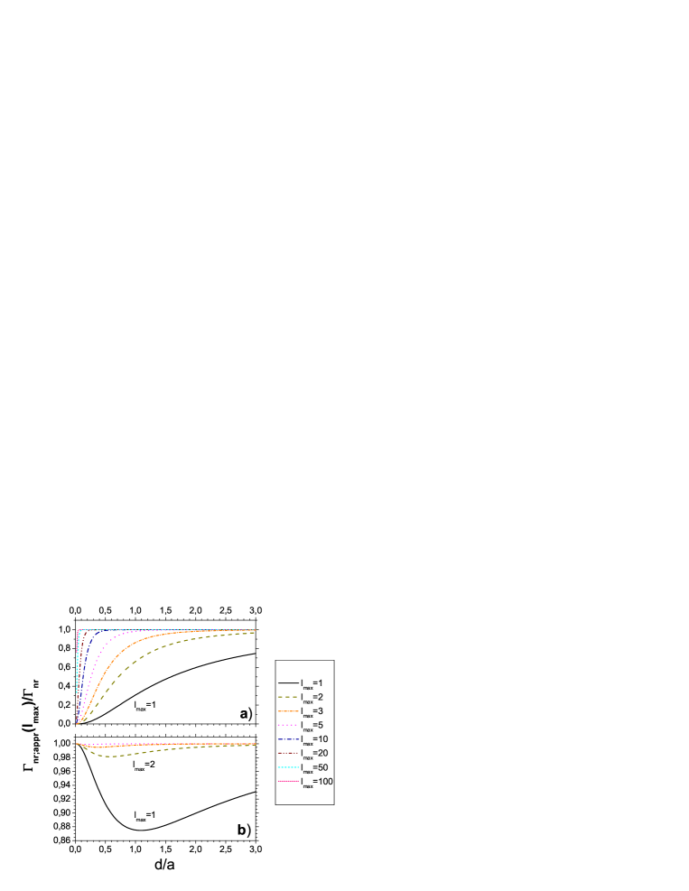
Figure 3:

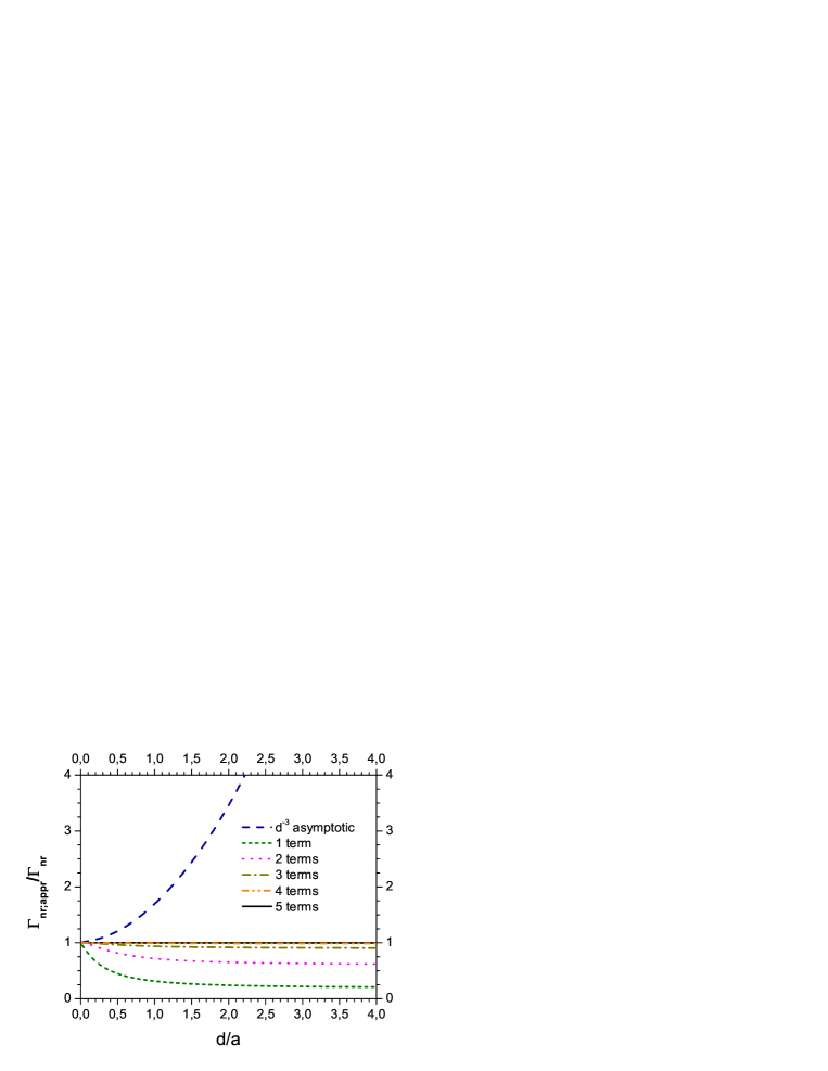
Figure 4:

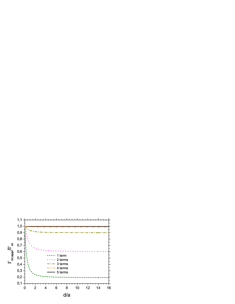
Figure 5:

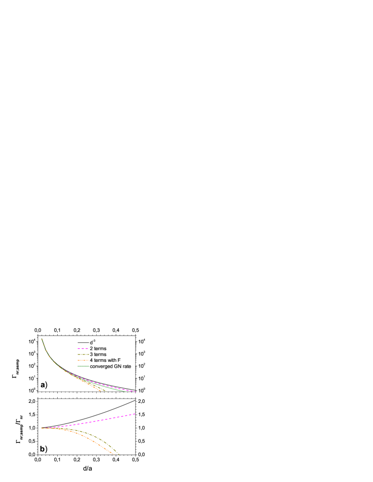
Figure 6:

References

- [1] Dubertret, B.; Calame, M.; Libchaber, A. J. Single-mismatch detection using gold-quenched fluorescent oligonucleotides. Nat. Biotechnol. 2001, 19, 365-370.
- [2] Maxwell, D. J.; Taylor, J. R.; Nie, S. Self-assembled nanoparticle probes for recognition and detection of biomolecules. J. Am. Chem. Soc. 2002, 124, 9606-9612.
- [3] Dulkeith, E.; Morteani, A. C.; Niedereichholz, T.; Klar, T. A.; Feldmann, J.; Levi, S. A.; van Veggel, F. C. J. M.; Reinhoudt, D. N.; Möller, M.; Gittins, D. I. Fluorescence quenching of dye molecules near gold nanoparticles: Radiative and nonradiative effects. Phys. Rev. Lett. 2002, 89, 203002.
- [4] Lakowicz, J. R. Radiative decay engineering 5: metal-enhanced fluorescence and plasmon emission. Anal. Biochem. 2005, 337, 171-194.
- [5] Yun, C. S.; Javier, A.; Jennings, T.; Fisher, M.; Hira, S.; Peterson, S.; Hopkins, B.; Reich, N. O.; Strouse, G. F. Nanometal surface energy transfer in optical rulers, breaking the FRET barrier. J. Am. Chem. Soc. 2005, 127, 3115-3119.
- [6] Jennings, T. L.; Schlatterer, J. C.; Singh, M. P.; Greenbaum, N. L.; Strouse, G. F. NSET molecular beacon analysis of hammerhead RNA substrate binding and catalysis. Nano Lett. 2006, 6, 1318-1324.
- [7] Soller, T.; Ringler, M.; Wunderlich, M.; Klar, T. A.; Feldmann, J.; Josel, H. P.; Markert, Y.; Nichtl, A.; Kürzinger, K. Radiative and nonradiative rates of phosphors attached to gold nanoparticles. Nano Lett. 2007, 7, 1941-1946.
- [8] Pons, T.; Medintz, I. L.; Sapsford, K. E.; Higashiya, S.; Grimes, A. F.; English, D. S.; Mattoussi, H. On the quenching of semiconductor quantum dot photoluminescence by proximal gold nanoparticles. Nano Lett. 2007, 7, 3157-3164.
- [9] Haldar, K. K.; Sen, T.; Patra, A. Metal Conjugated Semiconductor Hybrid Nanoparticle-Based Fluorescence Resonance Energy Transfer. J. Phys. Chem. C 2010, 114, pp 4869-4874.
- [10] Ruppin, R. Decay of an excited molecule near a small metal sphere. J. Chem. Phys. 1982, 76, 1681-1684.
- [11] Kim, Y. S.; Leung, P. T.; George, T. F. Classical decay rates for molecules in the presence of a spherical surface: A complete treatment. Surf. Sci. 1988, 195, 1-14.
- [12] Gersten, J.; Nitzan, A. Spectroscopic properties of molecules interacting with small dielectric particles. J. Chem. Phys. 1981, 75, 1139-1152.
- [13] Ford, G. W.; Weber, W. H. Electromagnetic interactions of molecules with metal surfaces. Phys. Rep. 1984, 113, 195-287.
- [14] Moroz, A. A recursive transfer-matrix solution for a dipole radiating inside and outside a stratified sphere. Ann. Phys. (NY) 2005, 315, 352-418.
- [15] Moroz, A. Spectroscopic properties of a two-level atom interacting with a complex spherical nanoshell. Chem. Phys. 2005, 317, 1-15.
- [16] Mertens, H.; Koenderink, A. F.; Polman, A. Plasmon-enhanced luminescence near noble-metal nanospheres: Comparison of exact theory and an improved Gersten and Nitzan model. Phys. Rev. B 2007, 76, 115123.
- [17] Moroz, A. Non-radiative decay of a dipole emitter close to a metallic nanoparticle: Importance of higher-order multipole contributions. Opt. Commun. 2010, 283, 2277-2287.
- [18] Chew, H. Transition rates of atoms near spherical surfaces. J. Chem. Phys. 1987, 87, 1355-1360.
- [19] Chew, H. Radiation and lifetimes of atoms inside dielectric particles. Phys. Rev. A 1988, 38, 3410-3416.
- [20] The source codes CHEWFS and CHEW could be downloaded from http://www.wave-scattering.com/chew.f and http://www.wave-scattering.com/chewfs.f. A brief description of the codes can be downloaded from http://www.wave-scattering.com/chew-man.pdf
-
[21]
Mathematical appendices for [12] (AIP Document No. PAPS JCP
SA-75-1139-32) available
as on-line supplementary material
(see also
http://atto.tau.ac.il/~nitzan/68-appendix.pdf). - [22] F77 source code based on Gersten and Nitzan theory [12, 21], which has been used to generate results here, could be downloaded from http://www.wave-scattering.com/gn.f.
- [23] Bohren C. F.; Huffman, D. R. Absorption and Scattering of Light by Small Particles, John Wiley & Sons, New York, 1988.
- [24] Palik, E. D., ed., Handbook of Optical Constants of Solids; Academic Press: New York, 1985.
- [25] A comparison of the respective analytic terms with their short-distance asymptotic could be downloaded from http://www.wave-scattering.com/Coefasmp.txt.
- [26] Bharadwaj, P.; Novotny, L. Spectral dependence of single molecule fluorescence enhancement. Opt. Express 2007, 15, 14266-14274.
- [27] Moroz, A. Electron mean-free path in metal coated nanowires. J. Opt. Soc. Am. B 2011, 28, 1130-1138.
- [28] Moroz, A. Localized resonances of composite particles. J. Phys. Chem. C 2009, 113, 21604-21610.
- [29] Moroz, A. Depolarization field of spheroidal particles. J. Opt. Soc. Am. B 2009, 26, 517-527.
- [30] Prudnikov, A. P.; Brychkov; Yu, A.; Marichev, O. I. Integrals and Series, 2nd ed; Gordon and Breach: London, 1988.