Abstract

We suggest a parameterization of the matrix element for $\bar{B}^{0}\to D^{*+}\omega\pi^{-}$ decay using kinematic variables convenient for experimental analysis. The contributions of intermediate $\omega\pi$- and $D^{**}$-states up to spin 3 have been taken into account. The angular distributions for each discussed hypothesis have been obtained and analysed using Monte Carlo simulation.

1 Introduction

The discovery of excited $D$-states (referred to as $D^{**}$-states) stimulates interest in their spectroscopy and $D^{**}\to D^{(*)}\pi$ decay properties. There are four $P$-wave states, which are usually labeled $D^{*}_{0}$ ($J^{P}_{j_{q}}=0^{+}_{1/2}$), $D^{\prime}_{1}$ ($J^{P}_{j_{q}}=1^{+}_{1/2}$), $D_{1}$ ($J^{P}_{j_{q}}=1^{+}_{3/2}$), $D^{*}_{2}$ ($J^{P}_{j_{q}}=2^{+}_{3/2}$), where $J$ is the spin of the meson and $j_{q}$ is the total angular momentum of a light quark $q=(u,d)$, which is the sum of the orbital momentum $l$ and the light quark spin $s_{q}$. In the heavy quark limit, the angular momentum $j_{q}$ is a good quantum number. Conservation of parity and angular momentum imposes constraints on the strong decays of the $D^{**}$ to $D^{(*)}\pi$. Two states with $j_{q}=1/2$ decay to the $D^{(*)}\pi$-state in $S$-wave while two other with $j_{q}=3/2$ decay in $D$-wave. Since the decay width $\Gamma\sim{\mathbf{Q}}^{2L+1}$, where ${\mathbf{Q}}$ is the magnitude of the daughter particle momentum, $L$ is the orbital momentum between decay products, and $\mathbf{Q}$ is small, $D_{1}$ and $D^{*}_{2}$ have small decay width of about $20$ MeV, but $D^{*}_{0}$ and $D^{\prime}_{1}$ are expected to be quite broad with decay width of about $300$ MeV [1, 2].

A further study of these states will allow a more in-depth comparison to be made with theoretical predictions such as Heavy Quark Effective Theory (HQET) [3, 4] and QCD sum rules [5]. The last experimental studies of $D^{**}$ mesons were performed in $B^{-}\to D^{(*)+}\pi^{-}\pi^{-}$ [6, 7] and $\bar{B}^{0}\to D^{0}\pi^{+}\pi^{-}$ [8] decays. These states have also been studied in semileptonic $B$-decays [9]. Thus, understanding of their properties is significant for reducing uncertainties in the measurement of semileptonic decays and determination of the Cabibbo-Kobayashi-Maskawa (CKM) [10] matrix elements $|V_{cb}|$ and $|V_{ub}|$.

$D^{**}$-states can be also produced in other hadronic $B$ decays, e.g., $B\to D^{*}\omega\pi$. Here, $D^{**}$ production is described by the $W$ vertex instead of the transition Isgur-Wise functions [3], which describe these states in the $D^{(*)}\pi\pi$ modes. This channel was first observed by the CLEO [11] and BaBar [12] collaborations, the latter finding an enhancement in $D^{*}\pi$ mass due to the broad $D_{1}(2430)^{0}$-state, representing a $P$-wave of a $D$ meson.

Let us note that light mesons decaying to the $\omega\pi$ final state (e.g., $\rho(1450)$, $b_{1}(1235)$ and their excitations) appear in the color-favored mode of this process. Thus, a possible contribution of these resonant structures to the total branching fraction can be measured. The $\rho(1450)$-resonance, dominant in this mode, was observed by both collaborations [11, 12], but the $b_{1}(1235)$-state was not observed in this channel.

An amplitude of three-body decay can be written as a sum of the contributions corresponding to the quasi-two-body resonances [6, 7, 8]. Analysing experimental data one has to determine relative amplitudes and phases of different intermediate states. To do this, one needs the amplitudes expressed via kinematic variables convenient for Dalitz plot analysis. These expressions can be used for optimization of selection criteria and creation of efficient Monte-Carlo generators.

2 The general method

A weak $B(0^{-})\to R(J^{P})1^{-}$ decay amplitude (for $J>0$) includes three independent terms while a strong $R(J^{P})\to 1^{-}0^{-}$ amplitude can have one or two independent terms. We can parameterize a decay matrix element using a set of different independent bases. In general, we can use the basis of covariant amplitudes or helicity basis etc. Since the real particles $D_{1}$ and $D^{\prime}_{1}$ are expected to be close to the pure $j_{q}=3/2$- and $j_{q}=1/2$-states and their decays have particular orbital momenta, it is convenient to use the basis of amplitudes describing decay with fixed angular orbital momenta in the $B$ and resonance rest frames.

In this paper we use an isobar model formulation in which our decay is described by a coherent sum of a number of quasi-two-body amplitudes. The amplitudes can be subdivided into two channels. The effective Hamiltonian for Cabibbo-favored decays can be reduced to the color-favored and color-suppressed forms [13, 14]:

$$H_{CF}\, = \,\frac{G_{F}}{\sqrt{2}}V_{cb}V^{*}_{ud}(a_{1}(\bar{c}\Gamma_{\mu}b)(\bar{u}\Gamma^{\mu}d)+C_{2}H^{8}_{w}){,}$$

$$H_{CS}\, = \,\frac{G_{F}}{\sqrt{2}}V_{cb}V^{*}_{ud}(a_{2}(\bar{c}\Gamma_{\mu}d)(\bar{u}\Gamma^{\mu}b)+C_{1}\tilde{H}^{8}_{w}){,}$$ (1)

where $G_{F}$ is the Fermi constant, $C_{1}$ and $C_{2}$ are the Wilson coefficients and $\Gamma_{\mu}=\gamma_{\mu}(1-\gamma_{5})$. The coefficients $a_{1}=C_{1}+C_{2}/N$ and $a_{2}=C_{2}+C_{1}/N$, where $N$ is an effective number of colors. The terms $H^{8}_{w}=\frac{1}{2}\sum^{8}_{a=1}(\bar{c}\lambda^{a}\Gamma_{\mu}b)(\bar{u}\lambda^{a}\Gamma^{\mu}d)$ and $\tilde{H}^{8}_{w}=\frac{1}{2}\sum^{8}_{a=1}(\bar{c}\lambda^{a}\Gamma_{\mu}d)(\bar{u}\lambda^{a}\Gamma^{\mu}b)$ ($\lambda^{a}$ are the Gell-Mann matrices), involving color-octet currents, generate non-factorized contributions. The other non-factorization source is the non-factorized matrix element of the product of the color-singlet currents. It includes loop current-current terms. The color-favored and color-suppressed channels are shown in Fig. 1. We show tree diagrams only, however, not all the intermediate states are described by them. In this paper we do not apply the factorization method but consider all intermediate resonant contributions up to spin $3$ allowed by the momentum-parity conservation.

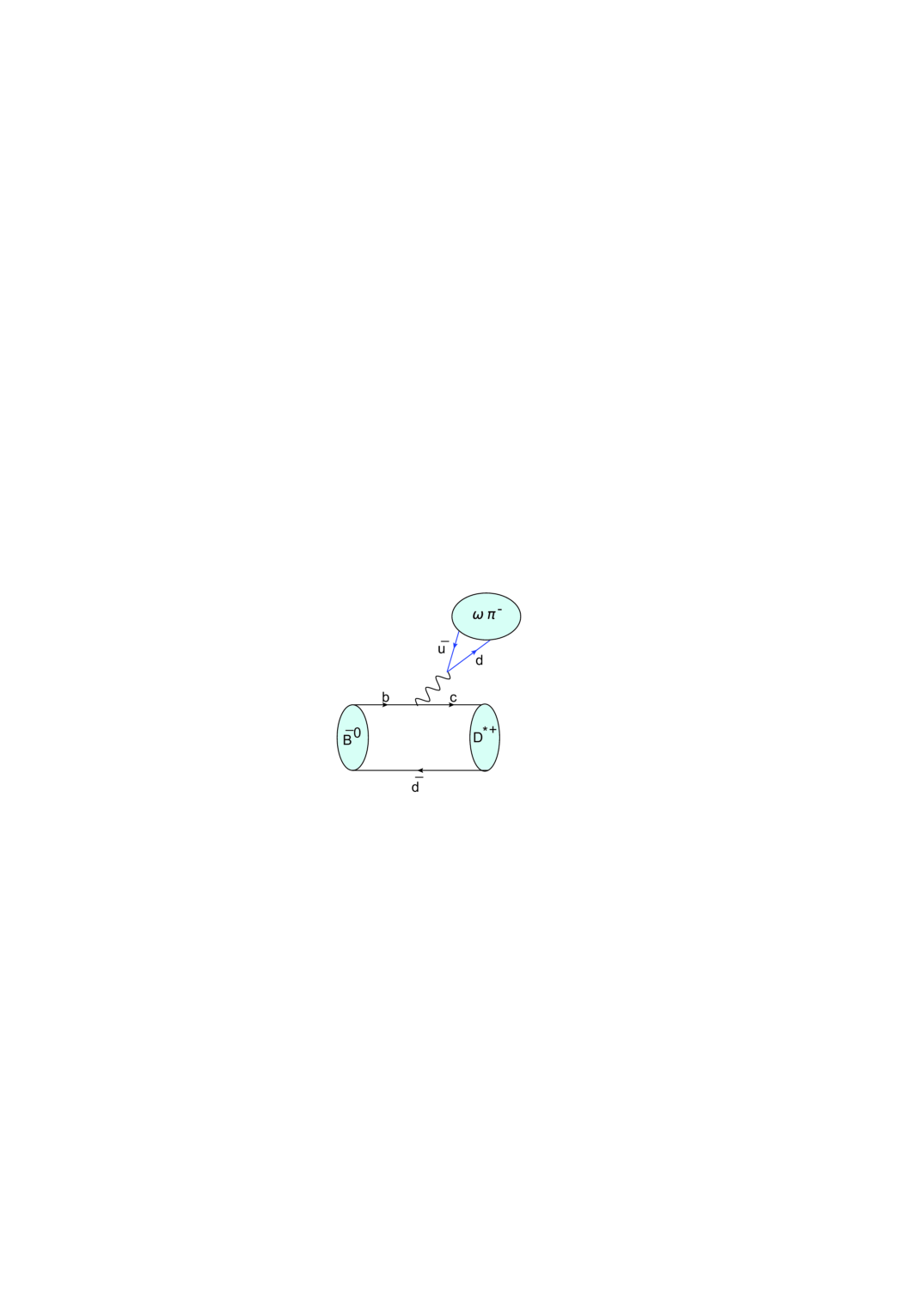
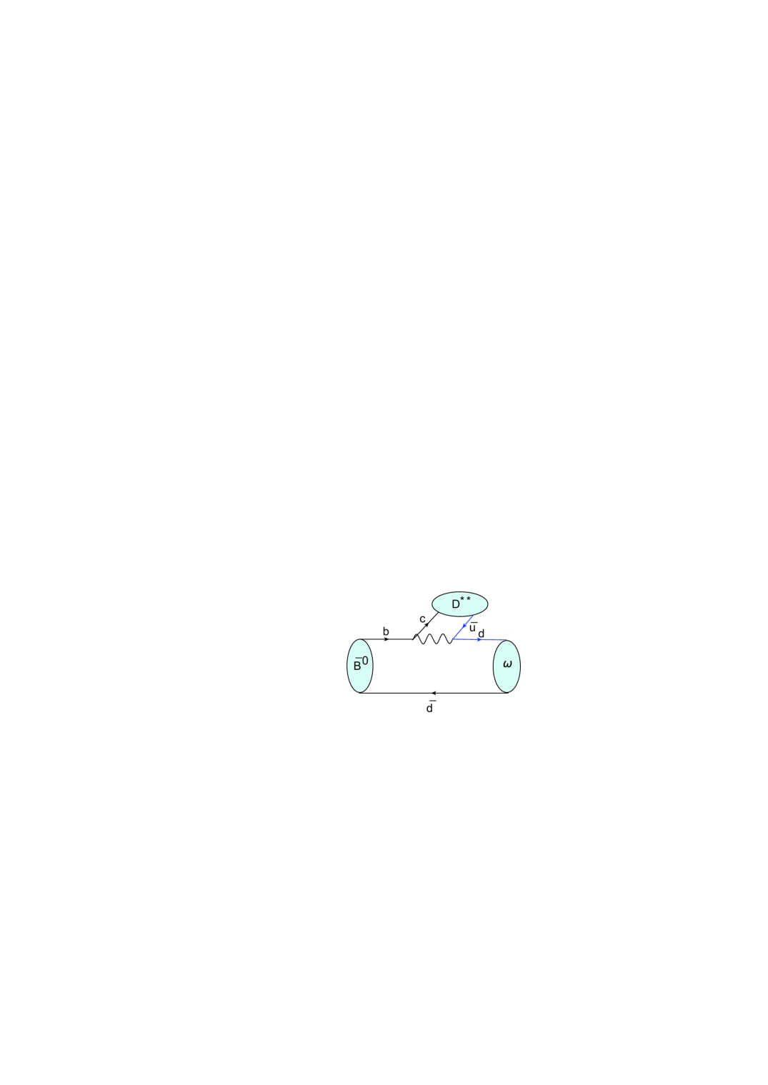
a)	b)

Figure 1: a) Color-favored and b) color-suppressed channel.

The color-favored term receives a contribution from the $\omega\pi$-resonances, e.g., $\rho(1450)$ and $b_{1}(1235)$. Since these resonances are broad, this channel allows factorization to be precisely tested [15]. The color-suppressed term receives a contribution from the $D^{**}$-states, which are $P$- and $D$-wave excitations of the $c\bar{u}$ states.

Let us consider briefly the spectroscopy of the $D$-wave $c\bar{u}$ excitations. We have $J^{P}_{j_{u}}=1^{-}_{3/2}$-, $J^{P}_{j_{u}}=2^{-}_{3/2}$-, $J^{P}_{j_{u}}=2^{-}_{5/2}$-, and $J^{P}_{j_{u}}=3^{-}_{5/2}$ states. Again, as discussed above, two states with $j_{u}=3/2$ decay to the $D^{(*)}\pi$-state in $P$-wave and two other with $j_{u}=5/2$ decay in $F$-wave.

Observable $c\bar{u}$-states with the same $J^{P}=1^{+}$ ($J^{P}=2^{-}$) quantum numbers are two linear combinations of pure $j_{u}=1/2$ ($j_{u}=3/2$)- and $j_{u}=3/2$ ($j_{u}=5/2$)-states. Thus, the physical $D_{1}$ and $D^{\prime}_{1}$-states are as follows:

$$|D_{1}>\, = \,\sin\vartheta_{1}\,|j_{u}=1/2>\,+\,\cos\vartheta_{1}\,e^{-i\vartheta_{2}}\,|j_{u}=3/2>{,}$$

$$|D^{\prime}_{1}>\, = \,\cos\vartheta_{1}\,|j_{u}=1/2>\,-\,\sin\vartheta_{1}\,e^{i\vartheta_{2}}\,|j_{u}=3/2>{,}$$

where $\vartheta_{1}$ and $\vartheta_{2}$ are mixing angles.

Let us discuss kinematic properties of the considered process. In the final state we have six particles, namely, $D^{0}$ and $\pi^{+}$ from the $D^{*+}$ decay, $\pi^{+}$, $\pi^{-}$ and $\pi^{0}$ from the $\omega$ decay and $\pi^{-}$ from the $\bar{B}^{0}$ decay. The $\bar{B}^{0}$ decay is described by two invariant masses squared of the $D^{*}\pi$ ($m^{2}_{D^{*}\pi}$) and $\omega\pi$ ($m^{2}_{\omega\pi}$) systems, the one corresponding to resonance mass labeled as $q^{2}$.

The $\omega$ decay is described by five variables. We use invariant masses squared $M^{2}_{0}=(P_{+}+P_{-})^{2}$ and $M^{2}_{+}=(P_{+}+P_{0})^{2}$ (here $P_{i}$ is a $4$-momentum of the pion $\pi^{i}$ from the $\omega$ decay, $i=\pm,0$), the azimuthal angle of the $\pi^{0}$ in the $\omega$ decay plane, and two angles (polar $\theta$ and azimuthal $\phi$) for a vector $\vec{n}$ normal to the $\omega$ decay plane. Let us note that the $\omega\to\pi\pi\pi$ decay proceeds through two mechanisms. The first one involves an intermediate $\rho$-meson. Experimental studies of the $e^{+}e^{-}\to 3\pi$ reaction have confirmed the Gell-Mann-Sharp-Wagner suggestion [16] that the $\omega\to 3\pi$ transition is dominated by this contribution. The second mechanism represents the non-resonant contribution. This contact contribution can not be excluded because interference between these mechanisms leads to a sizeable effect in the decay rate.

The $D^{*+}$ decay is described by two variables. We use polar $\beta$ and azimuthal $\psi$ angles for the $D^{0}$ momentum in the $D^{*+}$ rest frame. For further applications we assume the width of the $D^{*}$-meson to be negligible ($\Gamma_{D^{*+}}\approx 0.1\,{\rm MeV}\ll m_{D^{*+}}-(m_{D^{0}}+m_{\pi^{+}})\approx 10\,{\rm MeV}$). To describe the intermediate resonance decay, we use polar $\xi$ and azimuthal $\zeta$ angles for the daughter particle momentum in the resonance rest frame. The polar angle $\xi$ is expressed via the invariant mass squared $m^{2}_{D^{*}\pi}$ for the $\omega\pi$-states and $m^{2}_{\omega\pi}$ for the $D^{*}\pi$-states. Moreover, the matrix element does not depend on the azimuthal angle $\zeta$ for the $\omega\pi$- as well as for the $D^{*}\pi$-states.

A further definition of angles depends on the decay channel. Figure 2 shows the decay scheme and definition of the angles for the $\omega\pi$-resonances.

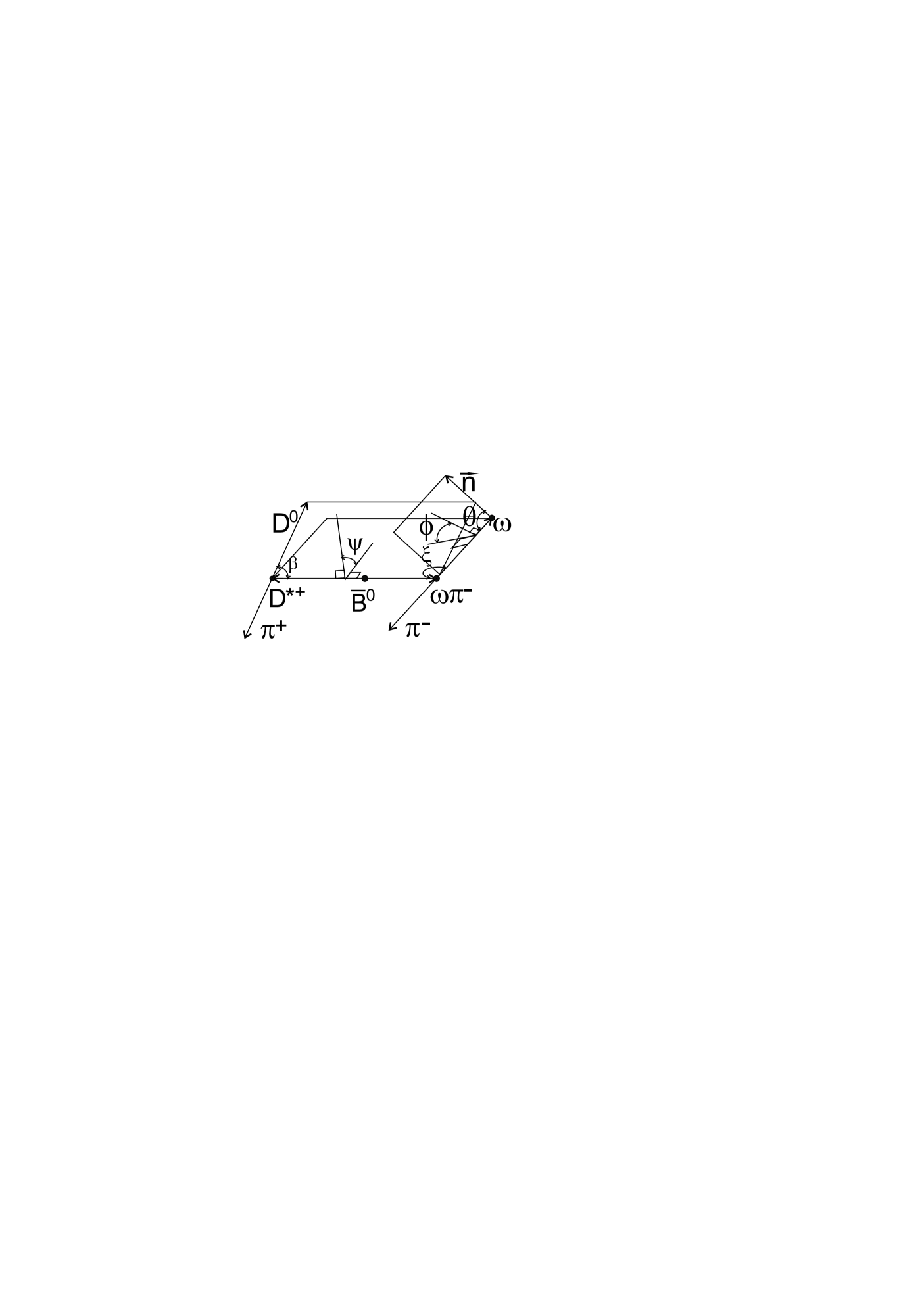
Figure 2: Complete visual definition of the angles for the $\omega\pi$-resonances. The angles $\theta$ and $\phi$ are defined in the $\omega$ rest frame, the angles $\beta$ and $\psi$ are defined in the $D^{*}$ rest frame and the angle $\xi$ is defined in the $\omega\pi$ rest frame.

Figures 3 and 4 define these angles using momentum variables for the $\omega\pi$- and $D^{*}\pi$-resonances, respectively. The notations are as follows: the variables $p$, $Q$, $l$, $q$ are the four-momenta of the $\omega$-, $D^{*}$-, $D$-meson and an intermediate resonance, respectively, while $\mathbf{p}$, $\mathbf{Q}$, $\mathbf{l}$, $\mathbf{q}$ are the magnitudes of their three-momenta in the mother particle rest frames. In Figs. 3, 4 the directions of these momenta define angular variables $\theta$ and $\phi$ in the $\omega$ rest frame, $\beta$ and $\psi$ in the $D^{*}$ rest frame and $\xi$ in the resonance rest frame.

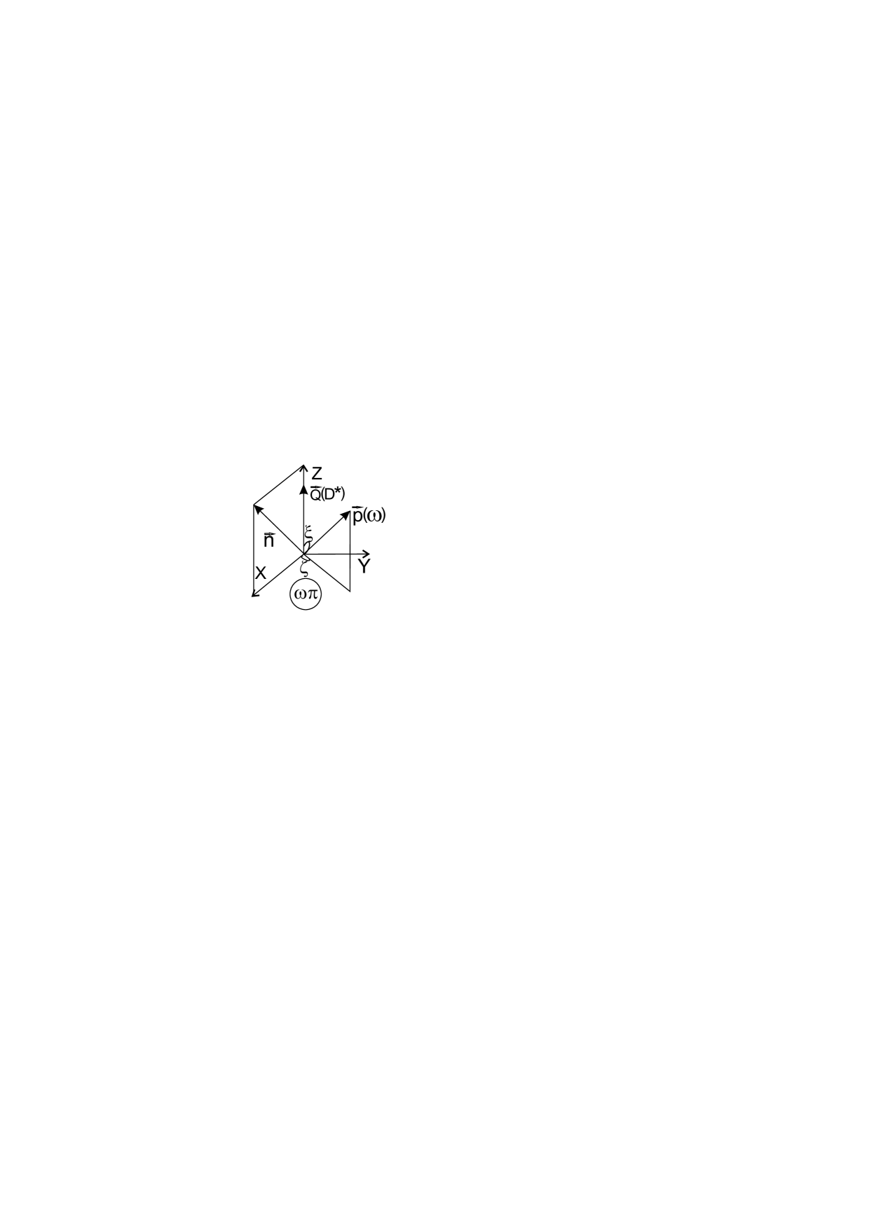
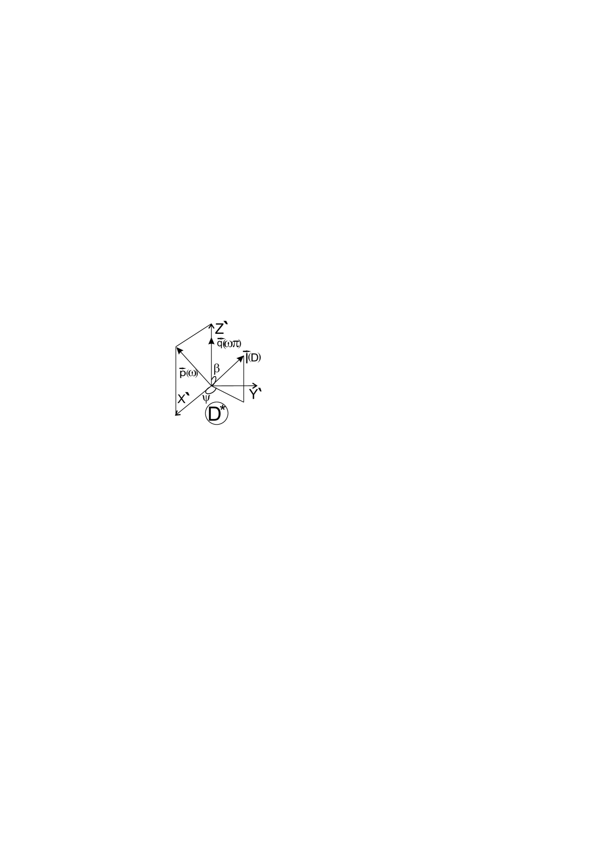
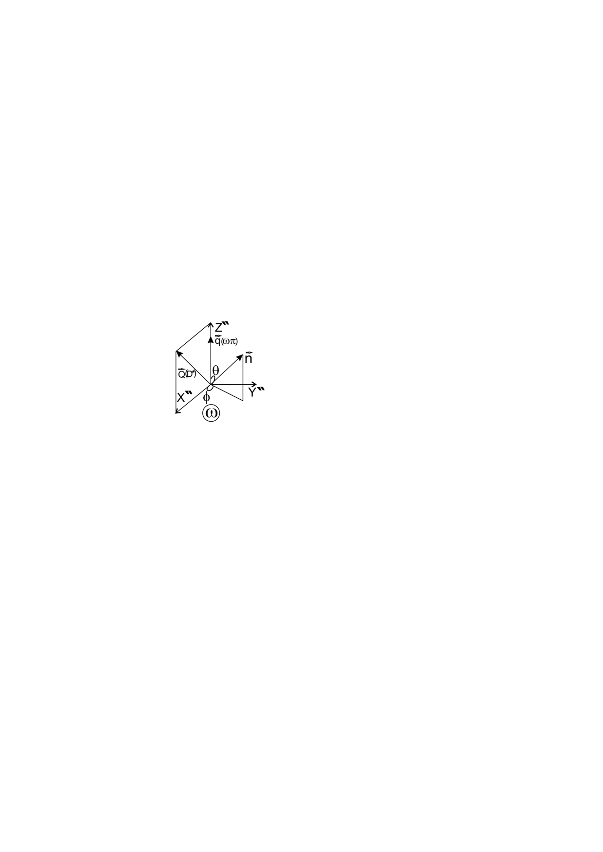
a)	b)	c)

Figure 3: Definition of the angles for the $\omega\pi$-resonances. Color-favored channel. a) The $\omega\pi$ rest frame, b) the $D^{*}$ rest frame and c) the $\omega$ rest frame.

a)	b)	c)

Figure 4: Definition of the angles for the $D^{**}$-resonances. Color-suppressed channel. a) The $D^{**}$ rest frame, b) the $\omega$ rest frame and c) the $D^{*}$ rest frame.

In this paper each compound particle is described by a relativistic Breit-Wigner (BW) with a $q^{2}$-dependent width. Such an approach is not exact since it does not take into account final state interactions and is neither analytic nor unitary. Nevertheless, it describes the main features of the amplitude behaviour and allows one to find and distinguish the contributions of different quasi-two-body intermediate states. Thus, the denominator of the BW propagator is:

$$D_{R}(q^{2})\,=\,q^{2}-m^{2}_{R}+im_{R}\Gamma_{R}(q^{2}){.}$$ (2)

It corresponds to the intermediate resonance $R$ with mass $m_{R}$ and $q^{2}$-dependent width $\Gamma_{R}$. The numerator of the propagator is to be the sum over polarizations of the resonance and depends on its spin.

3 $\omega\pi$-resonances

We consider such $\omega\pi$-states, which can be combined to $J^{P}=0^{-}$-, $J^{P}=1^{+}$ ($b_{1}(1235)$)-, $J^{P}=1^{-}$ ($\rho(1450)$)-, $J^{P}=2^{-}$-, $J^{P}=2^{+}$- and $J^{P}=3^{-}$($\rho_{3}(1690)$)-states. Let us note that $J^{P}=0^{-}$, $J^{P}=2^{-}$ and $J^{P}=2^{+}$ charged states, which decay to the $\omega\pi$-final system, have not yet been observed at the present time [2]. Such states have the isotopic quantum numbers $I^{G}=1^{+}$. It is natural to assume that these states are members of the $b$ and $\rho$-families.

The matrix element for production of the $J^{P}=0^{-}$ intermediate state (labeled as $\rho_{0}$) is given by:

$$M_{\bar{B}\to D^{*}\rho_{0}}\,=\,\frac{G_{F}}{\sqrt{2}}V_{cb}V^{*}_{ud}<D^{*}\rho_{0}|(\bar{u}\Gamma_{\mu}d)(\bar{c}\Gamma^{\mu}b)|\bar{B}>{,}$$ (3)

Parameterizing this amplitude in the covariant form, we have:

$$M_{\bar{B}\to D^{*}\rho_{0}}\,=\,\frac{G_{F}}{\sqrt{2}}V_{cb}V^{*}_{ud}g_{\rho_{0}}F_{P}(q^{2})(\varepsilon^{*}q){,}$$ (4)

where $\varepsilon_{\mu}$ is a polarization vector of $D^{*}$, $g_{\rho_{0}}=a_{1}f_{\rho_{0}}$, $f_{\rho_{0}}$ is a weak decay constant of the $\rho_{0}$ and $F_{P}(q^{2})$ is a transition form factor.

The strong amplitude for the $\rho_{0}$-decay is presented as follows:

$$M_{\rho_{0}\to\omega\pi}\,=\,\tilde{g}_{\rho_{0}\omega\pi}\tilde{F}_{P}(q^{2},p^{2})(v^{*}q){,}$$ (5)

where $v_{\mu}$ is a polarization vector of $\omega$, $\tilde{g}_{\rho_{0}\omega\pi}$ is a coupling constant and $\tilde{F}_{P}(q^{2},p^{2})$ is a transition form factor. The amplitude describing the $\omega$ decay comprises the contributions from the intermediate $\rho$-meson and $3\pi$ phase space:

$$M_{\omega\to 3\pi}\,=g_{\omega\rho\pi}(p^{2})\left(a_{3\pi}\,+\,\sum_{i=\pm,0}\frac{g_{\rho\pi\pi}}{D_{\rho^{i}}(M^{2}_{i})Z(M^{2}_{i})}\right)\sqrt{\Delta(p,P_{+},P_{0})}(nv){,}$$ (6)

where

$$n^{\mu}\,=\,\frac{\epsilon^{\mu\nu\rho\sigma}P_{+\nu}P_{0\rho}p_{\sigma}}{\sqrt{\Delta(p,P_{+},P_{0})}}$$ (7)

is a unit 4-vector normal to the $\omega$ decay plane and $\Delta(p,P_{+},P_{0})$ is the Kibble determinant. Other notations are described in the Appendix. Here and further $\epsilon_{\mu\nu\rho\sigma}$ is the Levi-Civita symbol and $\epsilon_{0123}=+1$. The amplitude corresponding to the $D^{*}$ decay is

$$M_{D^{*}\to D\pi}\,=\,g_{D^{*}D\pi}(\varepsilon l){.}$$ (8)

The factor

$$g_{D^{*}D\pi}(Q^{2})g_{\omega\rho\pi}(p^{2})\left(a_{3\pi}\,+\,\sum_{i=\pm,0}\frac{g_{\rho\pi\pi}}{D_{\rho^{i}}(M^{2}_{i})Z(M^{2}_{i})}\right)\frac{\sqrt{\Delta(p,P_{+},P_{0})}}{D_{D^{*}}(Q^{2})D_{\omega}(p^{2})}\mathbf{l}$$ (9)

is common for all intermediate states, and $\omega$-decay part can be expressed via the phase integral $W(p^{2})$, presented in the Appendix.

The total rate for $B\to D^{*}\omega\pi$ decay expressed via the branching fraction $\mathcal{B}_{D^{*+}\to D^{0}\pi^{+}}$ and the phase integral $W(p^{2})$ can be presented as follows:

$$d\Gamma\, =\,\frac{6\mathcal{B}_{D^{*+}\to D^{0}\pi^{+}}}{(4\pi)^{10}m^{2}_{B}}\,\frac{|M|^{2}\mathbf{p}\mathbf{Q}}{\sqrt{q^{2}}}\,\frac{W(p^{2})}{|D_{\omega}(p^{2})|^{2}}\,dp^{2}\,\,(d\cos\theta\,d\phi)\,(d\cos\beta\,d\psi)\,(dq^{2}\,d\cos\xi){,}$$ (10)

where $m_{B}$ is a $B$-meson mass, and the matrix element $M$ describes particular dependencies for the different intermediate channels.

The matrix element for the $\bar{B}\to D^{*}R_{J}$ transition, where $R_{J}$ is the intermediate resonance with the integer total spin $J$, can be parameterized in terms of the amplitudes with the definite angular orbital momentum $L$ as follows:

$$M_{\bar{B}\to D^{*}R_{J}}\, =\,\frac{G_{F}}{\sqrt{2}}V_{cb}V^{*}_{ud}\,g_{J}\,\left[\vphantom{\frac{1}{f_{J,J+1}}}C_{J}\epsilon^{\mu\nu\rho\sigma}\varepsilon^{{}^{\prime}*(J)}_{\mu}\varepsilon^{*}_{\nu}q_{\rho}Q_{\sigma}F_{L=J}(q^{2})+\right.$$

$$\left.{}+im^{2}_{B}C_{J-1}((\varepsilon^{{}^{\prime}*(J)}\varepsilon^{*})-\frac{1}{f_{J,J-1}(q^{2})}(\varepsilon^{{}^{\prime}*(J)}Q)(\varepsilon^{*}q))F_{L=J-1}(q^{2})+\right.$$

$$\left.{}+iC_{J+1}((\varepsilon^{{}^{\prime}*(J)}Q)(\varepsilon^{*}q)-f_{J,J+1}(q^{2})(\varepsilon^{{}^{\prime}*(J)}\varepsilon^{*}))F_{L=J+1}(q^{2})\vphantom{\frac{1}{f_{J,J+1}}}\right]{.}$$ (11)

Here, $C_{J}$ is the relative amplitude, which is in general complex; $F_{L}(q^{2})$ is a transition form factor corresponding to the orbital momentum $L$; $g_{1}=a_{1}f_{R}$, $f_{R}$ is a weak decay constant of the vector resonance, when $q^{2}=m^{2}_{R}$, $g_{2}=m_{B}g_{\bar{B}D^{*}R_{2}}$ and $g_{3}=m^{2}_{B}g_{\bar{B}D^{*}R_{3}}$ are appropriate coupling constants; $\varepsilon^{{}^{\prime}(J)}$ is a convolution of the resonant polarization tensor of rank $J$ and momentum $Q$

$$\varepsilon^{{}^{\prime}(J=1)}_{\mu} =\varepsilon^{{}^{\prime}}_{\mu},\quad\varepsilon^{{}^{\prime}(J=2)}_{\mu}=\varepsilon^{{}^{\prime}}_{\mu\alpha}Q^{\alpha}/m_{B},\quad\varepsilon^{{}^{\prime}(J=3)}_{\mu}=\varepsilon^{{}^{\prime}}_{\mu\alpha\beta}Q^{\alpha}Q^{\beta}/m^{2}_{B}{;}$$ (12)

$$f_{J,J\pm 1}(q^{2})=\frac{2m^{2}_{B}\mathbf{Q}^{2}}{m^{2}_{B}-m^{2}_{D^{*}}-q^{2}+2a_{J,J\pm 1}m_{D^{*}}\sqrt{q^{2}}}$$ (13)

and

$$a_{1,0}=-1,\quad a_{1,2}=+2,\quad a_{2,1}=-1,\quad a_{2,3}=+3/2,\quad a_{3,2}=-1,\quad a_{3,4}=+4/3{.}$$ (14)

The parameterization of the matrix element describing the resonance decay depends on its $J^{P}$ quantum numbers. Thus, resonances with $J^{P}=1^{-},2^{+},3^{-}$ are described by the following matrix element:

$$M_{R_{J}\to\omega\pi}\, =\,\tilde{g}_{J}\,\epsilon^{\mu\nu\rho\sigma}\tilde{\varepsilon}^{{}^{\prime}(J)}_{\mu}v^{*}_{\nu}q_{\rho}p_{\sigma}\tilde{F}_{L=J}(q^{2},p^{2}){,}$$ (15)

where $\tilde{g}_{1}=g_{R_{1}\omega\pi}$, $\tilde{g}_{2}=m_{R}g_{R_{2}\omega\pi}$ and $\tilde{g}_{3}=m^{2}_{R}g_{R_{3}\omega\pi}$ are appropriate coupling constants; $\tilde{F}_{L}(q^{2},p^{2})$ is a transition form factor and

$$\tilde{\varepsilon}^{{}^{\prime}(J=1)}_{\mu}=\varepsilon^{{}^{\prime}}_{\mu},\quad\tilde{\varepsilon}^{{}^{\prime}(J=2)}_{\mu}=\varepsilon^{{}^{\prime}}_{\mu\alpha}p^{\alpha}/m_{R},\quad\tilde{\varepsilon}^{{}^{\prime}(J=3)}_{\mu}=\varepsilon^{{}^{\prime}}_{\mu\alpha\beta}p^{\alpha}p^{\beta}/m^{2}_{R}{.}$$ (16)

The discussed resonances with $J^{P}=1^{+},2^{-}$ are described by the following matrix element:

$$M_{R_{J}\to\omega\pi}\, =\,\tilde{g}_{J}\,\left[\vphantom{\frac{1}{f_{J,J+1}}}\tilde{C}_{J-1}m^{2}_{R}((\tilde{\varepsilon}^{{}^{\prime}(J)}v^{*})-\frac{1}{\tilde{f}_{J,J-1}(q^{2})}(\tilde{\varepsilon}^{{}^{\prime}(J)}p)(v^{*}q))\tilde{F}_{L=J-1}(q^{2},p^{2})+\right.$$

$$\left.{}+\tilde{C}_{J+1}((\tilde{\varepsilon}^{{}^{\prime}(J)}p)(v^{*}q)-\tilde{f}_{J,J+1}(q^{2})(\tilde{\varepsilon}^{{}^{\prime}(J)}v^{*}))\tilde{F}_{L=J+1}(q^{2},p^{2})\vphantom{\frac{1}{f_{J,J+1}}}\right]{,}$$ (17)

where $\tilde{C}_{J}$ is the relative amplitude, which is in general complex, and

$$\tilde{f}_{J,J\pm 1}(q^{2})\,=\,\frac{2q^{2}\mathbf{p}^{2}}{q^{2}+p^{2}-m^{2}+2a_{J,J\pm 1}\sqrt{p^{2}q^{2}}}{,}$$ (18)

where $m$ is the charged pion mass.

Then we move from the covariant amplitudes to the expressions depending on the selected angles, which are defined in the intermediate particle rest frames.

4 $D^{**}$-resonances

The decay rate for the channel with $D^{**}$-resonance production has a form similar to (10). As already mentioned, in this case the angles $(\theta,\phi,\xi,\beta,\psi)$ differ from their analogues for the $\omega\pi$ states and are described in Fig. 4. Here we discuss two $J^{P}=1^{+}$-states and a $J^{P}=2^{+}$-state, which correspond to $P$-wave in the spectroscopy of the $c\bar{u}$ excitations as well as a $J^{P}=1^{-}$-state, two $J^{P}=2^{-}$-states and a $J^{P}=3^{-}$-state corresponding to the $D$-wave excited $c\bar{u}$-states. Pure $J^{P}_{j_{u}}=1^{+}_{1/2}$ ($J^{P}_{j_{u}}=2^{-}_{3/2}$)- and $J^{P}_{j_{u}}=1^{+}_{3/2}$ ($J^{P}_{j_{u}}=2^{-}_{5/2}$)-states decay to the $D^{*}\pi$ in $S$- ($P$-) wave and $D$- ($F$-) wave, respectively. As discussed above, observable $J^{P}=1^{+}$ ($J^{P}=2^{-}$) states can be a mixture of pure $j_{u}=1/2$ ($j_{u}=3/2$) and $j_{u}=3/2$ ($j_{u}=5/2$) states. This fact has to be taken into account for the total amplitude construction. The parameterization of the matrix elements for all $D^{**}$-states is similar to the case of the $\omega\pi$-states. However, mutual substitutions of the four-momenta $p$ and $Q$ and polarizations $\varepsilon_{\mu}$ and $v_{\mu}$ have to be made. The functions $f_{J,J\pm 1}(q^{2})$ and $\tilde{f}_{J,J\pm 1}(q^{2})$ for the $D^{**}$-states are as follows:

$$f_{J,J\pm 1}(q^{2})\, =\,\frac{2m^{2}_{B}\mathbf{p}^{2}}{m^{2}_{B}-p^{2}-q^{2}+2a_{J,J\pm 1}\sqrt{p^{2}q^{2}}}{,}$$ (19)

$$\tilde{f}_{J,J\pm 1}(q^{2})\, =\,\frac{2q^{2}\mathbf{Q}^{2}}{q^{2}+m^{2}_{D^{*}}-m^{2}+2a_{J,J\pm 1}m_{D^{*}}\sqrt{q^{2}}}{.}$$ (20)

5 Results

Using the technique described in the previous sections, we present the final expressions for matrix elements with different intermediate resonances. The total matrix element squared is as follows:

$$|M|^{2}\, =\,|M_{6}+M_{\rho_{0}}+M_{\rho(1450)}+M_{b_{1}(1235)}+M_{b_{2}}+M_{\rho_{2}}+M_{\rho_{3}}+M_{D_{1}}+M_{D^{\prime}_{1}}+M_{D^{*}_{2}}+$$

$$+M_{1^{-}_{3/2}}+M_{D_{2}}+M_{D^{\prime}_{2}}+M_{3^{-}_{5/2}}|^{2}{.}$$ (21)

Here, $M_{6}$ presents the non-resonant contributions to the matrix element. The amplitudes $M_{D_{1}}$ and $M_{D^{\prime}_{1}}$ are as follows:

$$M_{D_{1}}\, = \,\sin\vartheta_{1}\,|j_{u}=1/2>\,+\,\cos\vartheta_{1}\,e^{-i\vartheta_{2}}\,\,|j_{u}=3/2>{,}$$

$$M_{D^{\prime}_{1}}\, = \,\cos\vartheta_{1}\,|j_{u}=1/2>\,-\,\sin\vartheta_{1}\,e^{i\vartheta_{2}}\,|j_{u}=3/2>{,}$$ (22)

where $\vartheta_{1}$ and $\vartheta_{2}$ are mixing angles and similar expressions can be used for $2^{-}$-states.

The resonant matrix element can be presented as follows:

$$M_{R_{J}}\, =\,\frac{G_{F}}{\sqrt{2}}V_{cb}V^{*}_{ud}\frac{g_{\bar{B}D^{*}(\omega)R_{J}}\tilde{g}_{R_{J}\omega(D^{*})\pi}}{D_{R}(q^{2})}\sum_{L_{1}L_{2}}C_{L_{1}}\tilde{C}_{L_{2}}F_{L_{1}}(q^{2})\tilde{F}_{L_{2}}(q^{2})\mathcal{P}_{L_{1}L_{2}}A_{L_{1}L_{2}}{.}$$ (23)

Here, $L_{1}(L_{2})$ is the angular orbital momentum in the $\bar{B}^{0}(R)$ rest frame; $C_{L_{1}},\tilde{C}_{L_{2}}$ are relative amplitudes defined above, $\mathcal{P}_{L_{1}L_{2}}$ is the expression for the momentum dependence; $A_{L_{1}L_{2}}$ is the expression for the angular dependence. The expressions $\mathcal{P}_{L_{1}L_{2}}$ and $A_{L_{1}L_{2}}$ are combined in Table LABEL:t:LongTable for different intermediate states. The notations $c_{\alpha}=\cos\alpha$ and $s_{\alpha}=\sin\alpha$ are used. The functions $f_{J,J\pm 1}(q^{2})$ and $\tilde{f}_{J,J\pm 1}(q^{2})$ used in Table LABEL:t:LongTable are defined by (13) and (18) for the $\omega\pi$-resonances and by (19) and (20) for the $D^{**}$-resonances.

Resonance	$L_{1}$	$L_{2}$	$\mathcal{P}_{L_{1}L_{2}}$	$A_{L_{1}L_{2}}$
$\omega\pi$
$\rho_{0}$	$P$	$P$	$\frac{m_{B}\sqrt{q^{2}}}{m_{D^{*}}\sqrt{p^{2}}}\mathbf{p}\mathbf{Q}$	$c_{\theta}c_{\beta}$
$\rho(1450)$	$S$	$P$	$-im^{2}_{B}\sqrt{q^{2}}\mathbf{p}$	$-s_{\theta}s_{\phi}c_{\beta}s_{\xi}+s_{\theta}c_{\phi}s_{\beta}s_{\psi}-s_{\theta}s_{\phi}s_{\beta}c_{\psi}c_{\xi}$
	$P$	$P$	$m_{B}\sqrt{q^{2}}\mathbf{p}\mathbf{Q}$	$s_{\theta}s_{\phi}s_{\beta}s_{\psi}c_{\xi}+s_{\theta}c_{\phi}s_{\beta}c_{\psi}$
	$D$	$P$	$i\sqrt{q^{2}}f_{1,2}(q^{2})\mathbf{p}$	$2s_{\theta}s_{\phi}c_{\beta}s_{\xi}+s_{\theta}c_{\phi}s_{\beta}s_{\psi}-s_{\theta}s_{\phi}s_{\beta}c_{\psi}c_{\xi}$
$b_{1}(1235)$	$S$	$S$	$-im^{2}_{B}m^{2}_{R}$	$-c_{\theta}c_{\beta}c_{\xi}+s_{\theta}c_{\phi}c_{\beta}s_{\xi}-s_{\theta}s_{\phi}s_{\beta}s_{\psi}+$
				$+s_{\theta}c_{\phi}s_{\beta}c_{\psi}c_{\xi}+c_{\theta}s_{\beta}c_{\psi}s_{\xi}$
	$S$	$D$	$im^{2}_{B}\tilde{f}_{1,2}(q^{2})$	$2c_{\theta}c_{\beta}c_{\xi}-2s_{\theta}c_{\phi}c_{\beta}s_{\xi}-s_{\theta}s_{\phi}s_{\beta}s_{\psi}+$
				$+s_{\theta}c_{\phi}s_{\beta}c_{\psi}c_{\xi}+c_{\theta}s_{\beta}c_{\psi}s_{\xi}$
	$P$	$S$	$m^{2}_{R}m_{B}\mathbf{Q}$	$-c_{\theta}s_{\beta}s_{\psi}s_{\xi}+s_{\theta}s_{\phi}s_{\beta}c_{\psi}-s_{\theta}c_{\phi}s_{\beta}s_{\psi}c_{\xi}$
	$P$	$D$	$-m_{B}\tilde{f}_{1,2}(q^{2})\mathbf{Q}$	$2c_{\theta}s_{\beta}s_{\psi}s_{\xi}+s_{\theta}s_{\phi}s_{\beta}c_{\psi}-s_{\theta}c_{\phi}s_{\beta}s_{\psi}c_{\xi}$
	$D$	$S$	$im^{2}_{R}f_{1,2}(q^{2})$	$2c_{\theta}c_{\beta}c_{\xi}+s_{\theta}c_{\phi}c_{\beta}s_{\xi}-s_{\theta}s_{\phi}s_{\beta}s_{\psi}+$
				$+s_{\theta}c_{\phi}s_{\beta}c_{\psi}c_{\xi}-2c_{\theta}s_{\beta}c_{\psi}s_{\xi}$
	$D$	$D$	$-if_{1,2}(q^{2})\tilde{f}_{1,2}(q^{2})$	$-4c_{\theta}c_{\beta}c_{\xi}-2s_{\theta}c_{\phi}c_{\beta}s_{\xi}-s_{\theta}s_{\phi}s_{\beta}s_{\psi}+$
				$+s_{\theta}c_{\phi}s_{\beta}c_{\psi}c_{\xi}-2c_{\theta}s_{\beta}c_{\psi}s_{\xi}$

Resonance	$L_{1}$	$L_{2}$	$\mathcal{P}_{L_{1}L_{2}}$	$A_{L_{1}L_{2}}$
$\omega\pi$
$b_{2}$	$P$	$D$	$-\frac{i}{2}m^{3}_{B}\mathbf{p}^{2}\mathbf{Q}$	$s_{\theta}s_{\phi}c_{\beta}s_{2\xi}+s_{\theta}s_{\phi}s_{\beta}c_{\psi}c_{2\xi}-s_{\theta}c_{\phi}s_{\beta}s_{\psi}c_{\xi}$
	$D$	$D$	$\frac{1}{2}m^{2}_{B}\mathbf{p}^{2}\mathbf{Q}^{2}$	$s_{\theta}s_{\phi}s_{\beta}s_{\psi}+s_{\theta}c_{\phi}s_{\beta}c_{\psi}c_{\xi}$
	$F$	$D$	$\frac{i}{2}m_{B}f_{2,3}(q^{2})\mathbf{p}^{2}\mathbf{Q}$	$-3/2s_{\theta}s_{\phi}c_{\beta}s_{2\xi}+s_{\theta}s_{\phi}s_{\beta}c_{\psi}c_{2\xi}-s_{\theta}c_{\phi}s_{\beta}s_{\psi}c_{\xi}$
$\rho_{2}$	$P$	$P$	$\frac{i}{\sqrt{q^{2}}}m^{3}_{B}m^{2}_{R}\mathbf{p}\mathbf{Q}$	$c_{\theta}c_{\beta}(c^{2}_{\xi}-1/3)-1/2c_{\theta}s_{\beta}c_{\psi}s_{2\xi}-1/2s_{\theta}c_{\phi}c_{\beta}s_{2\xi}-$
				$-1/2s_{\theta}s_{\phi}s_{\beta}s_{\psi}c_{\xi}-s_{\theta}c_{\phi}s_{\beta}c_{\psi}(c^{2}_{\xi}-1/2)$
	$P$	$F$	$-\frac{i}{\sqrt{q^{2}}}m^{3}_{B}\tilde{f}_{2,3}(q^{2})\mathbf{p}\mathbf{Q}$	$-3/2c_{\theta}c_{\beta}(c^{2}_{\xi}-1/3)+3/4c_{\theta}s_{\beta}c_{\psi}s_{2\xi}-1/2s_{\theta}c_{\phi}c_{\beta}s_{2\xi}-$
				$-1/2s_{\theta}s_{\phi}s_{\beta}s_{\psi}c_{\xi}-s_{\theta}c_{\phi}s_{\beta}c_{\psi}(c^{2}_{\xi}-1/2)$
	$D$	$P$	$-\frac{m^{2}_{R}m^{2}_{B}}{2\sqrt{q^{2}}}\mathbf{p}\mathbf{Q}^{2}$	$c_{\theta}s_{\beta}s_{\psi}s_{2\xi}+s_{\theta}c_{\phi}s_{\beta}s_{\psi}c_{2\xi}-s_{\theta}s_{\phi}s_{\beta}c_{\psi}c_{\xi}$
	$D$	$F$	$\frac{m^{2}_{B}}{2\sqrt{q^{2}}}\tilde{f}_{2,3}(q^{2})\mathbf{p}\mathbf{Q}^{2}$	$-3/2c_{\theta}s_{\beta}s_{\psi}s_{2\xi}+s_{\theta}c_{\phi}s_{\beta}s_{\psi}c_{2\xi}-s_{\theta}s_{\phi}s_{\beta}c_{\psi}c_{\xi}$
	$F$	$P$	$-\frac{i}{\sqrt{q^{2}}}m^{2}_{R}m_{B}f_{2,3}(q^{2})\mathbf{p}\mathbf{Q}$	$-3/2c_{\theta}c_{\beta}(c^{2}_{\xi}-1/3)-1/2c_{\theta}s_{\beta}c_{\psi}s_{2\xi}+3/4s_{\theta}c_{\phi}c_{\beta}s_{2\xi}-$
				$-1/2s_{\theta}s_{\phi}s_{\beta}s_{\psi}c_{\xi}-s_{\theta}c_{\phi}s_{\beta}c_{\psi}(c^{2}_{\xi}-1/2)$
	$F$	$F$	$\frac{i}{\sqrt{q^{2}}}m_{B}f_{2,3}(q^{2})\tilde{f}_{2,3}(q^{2})\mathbf{p}\mathbf{Q}$	$9/4c_{\theta}c_{\beta}(c^{2}_{\xi}-1/3)+3/4c_{\theta}s_{\beta}c_{\psi}s_{2\xi}+3/4s_{\theta}c_{\phi}c_{\beta}s_{2\xi}-$
				$-1/2s_{\theta}s_{\phi}s_{\beta}s_{\psi}c_{\xi}-s_{\theta}c_{\phi}s_{\beta}c_{\psi}(c^{2}_{\xi}-1/2)$
$\rho_{3}$	$D$	$F$	$\frac{i}{\sqrt{q^{2}}}m^{4}_{B}\mathbf{p}^{3}\mathbf{Q}^{2}$	$1/3(s_{\theta}c_{\phi}s_{\beta}s_{\psi}-s_{\theta}s_{\phi}s_{\beta}c_{\psi}c_{\xi})(c^{2}_{\xi}-1/5)-$
				$-s_{\theta}s_{\phi}c_{\beta}s_{\xi}(c^{2}_{\xi}-1/5)+2/3s_{\theta}s_{\phi}s_{\beta}c_{\psi}c_{\xi}s^{2}_{\xi}$
	$F$	$F$	$\frac{m^{3}_{B}}{3\sqrt{q^{2}}}\mathbf{p}^{3}\mathbf{Q}^{3}$	$(s_{\theta}s_{\phi}s_{\beta}s_{\psi}c_{\xi}+s_{\theta}c_{\phi}s_{\beta}c_{\psi})(c^{2}_{\xi}-1/5)-2s_{\theta}s_{\phi}s_{\beta}s_{\psi}c_{\xi}s^{2}_{\xi}$
	$G$	$F$	$-\frac{i}{\sqrt{q^{2}}}m^{2}_{B}f_{3,4}(q^{2})\mathbf{p}^{3}\mathbf{Q}^{2}$	$1/3(s_{\theta}c_{\phi}s_{\beta}s_{\psi}-s_{\theta}s_{\phi}s_{\beta}c_{\psi}c_{\xi})(c^{2}_{\xi}-1/5)+$
				$+4/3s_{\theta}s_{\phi}c_{\beta}s_{\xi}(c^{2}_{\xi}-1/5)+2/3s_{\theta}s_{\phi}s_{\beta}c_{\psi}c_{\xi}s^{2}_{\xi}$

Resonance	$L_{1}$	$L_{2}$	$\mathcal{P}_{L_{1}L_{2}}$	$A_{L_{1}L_{2}}$
$D^{**}$
$1^{+}_{1/2}$	$S$	$S$	-$im^{2}_{B}m^{2}_{R}$	$-c_{\theta}c_{\beta}c_{\xi}+s_{\theta}c_{\phi}c_{\beta}s_{\xi}-s_{\theta}s_{\phi}s_{\beta}s_{\psi}+$
				$+s_{\theta}c_{\phi}s_{\beta}c_{\psi}c_{\xi}+c_{\theta}s_{\beta}c_{\psi}s_{\xi}$
	$P$	$S$	$m^{2}_{R}m_{B}\mathbf{p}$	$-s_{\theta}s_{\phi}c_{\beta}s_{\xi}-s_{\theta}s_{\phi}s_{\beta}c_{\psi}c_{\xi}+s_{\theta}c_{\phi}s_{\beta}s_{\psi}$
	$D$	$S$	$im^{2}_{R}f_{1,2}(q^{2})$	$2c_{\theta}c_{\beta}c_{\xi}+s_{\theta}c_{\phi}c_{\beta}s_{\xi}-s_{\theta}s_{\phi}s_{\beta}s_{\psi}+$
				$+s_{\theta}c_{\phi}s_{\beta}c_{\psi}c_{\xi}-2c_{\theta}s_{\beta}c_{\psi}s_{\xi}$
$1^{+}_{3/2}$	$S$	$D$	$im^{2}_{B}\tilde{f}_{1,2}(q^{2})$	$2c_{\theta}c_{\beta}c_{\xi}-2s_{\theta}c_{\phi}c_{\beta}s_{\xi}-s_{\theta}s_{\phi}s_{\beta}s_{\psi}+$
				$+s_{\theta}c_{\phi}s_{\beta}c_{\psi}c_{\xi}+c_{\theta}s_{\beta}c_{\psi}s_{\xi}$
	$P$	$D$	$-m_{B}\tilde{f}_{1,2}(q^{2})\mathbf{p}$	$2s_{\theta}s_{\phi}c_{\beta}s_{\xi}-s_{\theta}s_{\phi}s_{\beta}c_{\psi}c_{\xi}+s_{\theta}c_{\phi}s_{\beta}s_{\psi}$
	$D$	$D$	$-if_{1,2}(q^{2})\tilde{f}_{1,2}(q^{2})$	$-4c_{\theta}c_{\beta}c_{\xi}-2s_{\theta}c_{\phi}c_{\beta}s_{\xi}-s_{\theta}s_{\phi}s_{\beta}s_{\psi}+$
				$+s_{\theta}c_{\phi}s_{\beta}c_{\psi}c_{\xi}-2c_{\theta}s_{\beta}c_{\psi}s_{\xi}$
$2^{+}_{3/2}$	$P$	$D$	$-\frac{i}{2}m^{3}_{B}\mathbf{Q}^{2}\mathbf{p}$	$c_{\theta}s_{\beta}s_{\psi}s_{2\xi}+s_{\theta}c_{\phi}s_{\beta}s_{\psi}c_{2\xi}-s_{\theta}s_{\phi}s_{\beta}c_{\psi}c_{\xi}$
	$D$	$D$	$\frac{1}{2}m^{2}_{B}\mathbf{Q}^{2}\mathbf{p}^{2}$	$s_{\theta}s_{\phi}s_{\beta}s_{\psi}+s_{\theta}c_{\phi}s_{\beta}c_{\psi}c_{\xi}$
	$F$	$D$	$\frac{i}{2}m_{B}f_{2,3}(q^{2})\mathbf{Q}^{2}\mathbf{p}$	$-3/2c_{\theta}s_{\beta}s_{\psi}s_{2\xi}+s_{\theta}c_{\phi}s_{\beta}s_{\psi}c_{2\xi}-s_{\theta}s_{\phi}s_{\beta}c_{\psi}c_{\xi}$
$1^{-}_{3/2}$	$S$	$P$	$-im^{2}_{B}\sqrt{q^{2}}\mathbf{Q}$	$-c_{\theta}s_{\beta}s_{\psi}s_{\xi}+s_{\theta}s_{\phi}s_{\beta}c_{\psi}-s_{\theta}c_{\phi}s_{\beta}s_{\psi}c_{\xi}$
	$P$	$P$	$m_{B}\sqrt{q^{2}}\mathbf{Q}\mathbf{p}$	$s_{\theta}s_{\phi}s_{\beta}s_{\psi}c_{\xi}+s_{\theta}c_{\phi}s_{\beta}c_{\psi}$
	$D$	$P$	$i\sqrt{q^{2}}f_{1,2}(q^{2})\mathbf{Q}$	$2c_{\theta}s_{\beta}s_{\psi}s_{\xi}+s_{\theta}s_{\phi}s_{\beta}c_{\psi}-s_{\theta}c_{\phi}s_{\beta}s_{\psi}c_{\xi}$

Table 1: Summary of momentum and angular distributions for different intermediate states, which are described in this paper.

Resonance	$L_{1}$	$L_{2}$	$\mathcal{P}_{L_{1}L_{2}}$	$A_{L_{1}L_{2}}$
$D^{**}$
$2^{-}_{3/2}$	$P$	$P$	$\frac{i}{\sqrt{q^{2}}}m^{3}_{B}m^{2}_{R}\mathbf{Q}\mathbf{p}$	$c_{\theta}c_{\beta}(c^{2}_{\xi}-1/3)-1/2c_{\theta}s_{\beta}c_{\psi}s_{2\xi}-1/2s_{\theta}c_{\phi}c_{\beta}s_{2\xi}-$
				$-1/2s_{\theta}s_{\phi}s_{\beta}s_{\psi}c_{\xi}-s_{\theta}c_{\phi}s_{\beta}c_{\psi}(c^{2}_{\xi}-1/2)$
	$D$	$P$	$-\frac{m^{2}_{R}m^{2}_{B}}{2\sqrt{q^{2}}}\mathbf{Q}\mathbf{p}^{2}$	$s_{\theta}s_{\phi}c_{\beta}s_{2\xi}+s_{\theta}s_{\phi}s_{\beta}c_{\psi}c_{2\xi}-s_{\theta}c_{\phi}s_{\beta}s_{\psi}c_{\xi}$
	$F$	$P$	$-\frac{i}{\sqrt{q^{2}}}m^{2}_{R}m_{B}f_{2,3}(q^{2})\mathbf{Q}\mathbf{p}$	$-3/2c_{\theta}c_{\beta}(c^{2}_{\xi}-1/3)-1/2c_{\theta}s_{\beta}c_{\psi}s_{2\xi}+3/4s_{\theta}c_{\phi}c_{\beta}s_{2\xi}-$
				$-1/2s_{\theta}s_{\phi}s_{\beta}s_{\psi}c_{\xi}-s_{\theta}c_{\phi}s_{\beta}c_{\psi}(c^{2}_{\xi}-1/2)$
$2^{-}_{5/2}$	$P$	$F$	$-\frac{i}{\sqrt{q^{2}}}m^{3}_{B}\tilde{f}_{2,3}(q^{2})\mathbf{Q}\mathbf{p}$	$-3/2c_{\theta}c_{\beta}(c^{2}_{\xi}-1/3)+3/4c_{\theta}s_{\beta}c_{\psi}s_{2\xi}-1/2s_{\theta}c_{\phi}c_{\beta}s_{2\xi}-$
				$-1/2s_{\theta}s_{\phi}s_{\beta}s_{\psi}c_{\xi}-s_{\theta}c_{\phi}s_{\beta}c_{\psi}(c^{2}_{\xi}-1/2)$
	$D$	$F$	$\frac{m^{2}_{B}}{2\sqrt{q^{2}}}\tilde{f}_{2,3}(q^{2})\mathbf{Q}\mathbf{p}^{2}$	$-3/2s_{\theta}s_{\phi}c_{\beta}s_{2\xi}+s_{\theta}s_{\phi}s_{\beta}c_{\psi}c_{2\xi}-s_{\theta}c_{\phi}s_{\beta}s_{\psi}c_{\xi}$
	$F$	$F$	$\frac{i}{\sqrt{q^{2}}}m_{B}f_{2,3}(q^{2})\tilde{f}_{2,3}(q^{2})\mathbf{Q}\mathbf{p}$	$9/4c_{\theta}c_{\beta}(c^{2}_{\xi}-1/3)+3/4c_{\theta}s_{\beta}c_{\psi}s_{2\xi}+3/4s_{\theta}c_{\phi}c_{\beta}s_{2\xi}-$
				$-1/2s_{\theta}s_{\phi}s_{\beta}s_{\psi}c_{\xi}-s_{\theta}c_{\phi}s_{\beta}c_{\psi}(c^{2}_{\xi}-1/2)$
$3^{-}_{5/2}$	$D$	$F$	$\frac{i}{\sqrt{q^{2}}}m^{4}_{B}\mathbf{Q}^{3}\mathbf{p}^{2}$	$s_{\theta}c_{\phi}s_{\beta}s_{\psi}c_{\xi}s^{2}_{\xi}-4/15s_{\theta}c_{\phi}s_{\beta}s_{\psi}c_{\xi}+$
				$+1/3s_{\theta}s_{\phi}s_{\beta}c_{\psi}(c^{2}_{\xi}-1/5)-c_{\theta}s_{\beta}s_{\psi}s_{\xi}(c^{2}_{\xi}-1/5)$
	$F$	$F$	$\frac{m^{3}_{B}}{3\sqrt{q^{2}}}\mathbf{Q}^{3}\mathbf{p}^{3}$	$(s_{\theta}s_{\phi}s_{\beta}s_{\psi}c_{\xi}+s_{\theta}c_{\phi}s_{\beta}c_{\psi})(c^{2}_{\xi}-1/5)-2s_{\theta}s_{\phi}s_{\beta}s_{\psi}c_{\xi}s^{2}_{\xi}$
	$G$	$F$	$-\frac{i}{\sqrt{q^{2}}}m^{2}_{B}f_{3,4}(q^{2})\mathbf{Q}^{3}\mathbf{p}^{2}$	$s_{\theta}c_{\phi}s_{\beta}s_{\psi}c_{\xi}s^{2}_{\xi}-4/15s_{\theta}c_{\phi}s_{\beta}s_{\psi}c_{\xi}+$
				$+1/3s_{\theta}s_{\phi}s_{\beta}c_{\psi}(c^{2}_{\xi}-1/5)+4/3c_{\theta}s_{\beta}s_{\psi}s_{\xi}(c^{2}_{\xi}-1/5)$

6 Decay chain simulation

To demonstrate the angular distributions for each intermediate resonance in the $D^{*}\omega\pi$ final state, we generate $2\times 10^{6}$ $\bar{B}^{0}\to D^{*+}\omega\pi^{-}$ events according to the phase space distribution using the qq98 program package [17]. For a further study we fill profile angular spectra with the appropriate weight density functions for each resonant hypothesis, which have been obtained above.

A description of each vertex includes transition form factors. Since it is not yet possible to obtain these form factors from rigorous theoretical calculations, we rely on the simple phenomenological Blatt-Weisskopf model [18, 19]. For $L>0$ this simple form factor suppresses growth of the matrix element with final particle momentum. The Blatt-Weisskopf functions $B_{L}(x)$ are chosen as follows:

$$B_{L}(x)\,=\,\frac{x_{0}^{L+1}|h_{L}(x_{0})|}{x^{L+1}|h_{L}(x)|}{,}$$ (24)

where

$$h_{L}(x)\,=\,\frac{-i}{x}e^{i\left(x-\frac{\pi L}{2}\right)}\sum^{L}_{n=0}(-1)^{n}\frac{(L+n)!}{n!(L-n)!}(2ix)^{-n}$$ (25)

is a spherical Hankel function, $x=\mathbf{k}r$, $x_{0}=\mathbf{k}_{0}r$, $\mathbf{k},\,\mathbf{k}_{0}$ are the magnitudes of the daughter particle three-momentum in the mother particle rest frame for the case when the resonance four-momentum squared is equal to $q^{2}$ and $m^{2}_{R}$, respectively, and $r=1.6\,\mathrm{GeV}^{-1}$ is a hadron scale. According to our normalization, these functions are equal to one, when $\sqrt{q^{2}}=m_{R}$. Another common normalization gives $B_{L}(x)=1$ for $x=1$. The Blatt-Weisskopf functions corresponding to $L$ discussed here are given below for convenience:

$$B_{0}(x)\, =\,1{,}$$

$$B_{1}(x)\, =\,\sqrt{\frac{1+x^{2}_{0}}{1+x^{2}}}{,}$$

$$B_{2}(x)\, =\,\sqrt{\frac{(x^{2}_{0}-3)^{2}+9x^{2}_{0}}{(x^{2}-3)^{2}+9x^{2}}}{,}$$

$$B_{3}(x)\, =\,\sqrt{\frac{x^{2}_{0}(x^{2}_{0}-15)^{2}+9(2x^{2}_{0}-5)^{2}}{x^{2}(x^{2}-15)^{2}+9(2x^{2}-5)^{2}}}{,}$$

$$B_{4}(x)\, =\,\sqrt{\frac{(x^{4}_{0}-45x^{2}_{0}+105)^{2}+25x^{2}_{0}(2x^{2}_{0}-21)^{2}}{(x^{4}-45x^{2}+105)^{2}+25x^{2}(2x^{2}-21)^{2}}}{.}$$ (26)

a1)	a2)	a3)
b1)	b2)	b3)
c1)	c2)	c3)
d1)	d2)	d3)

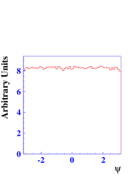
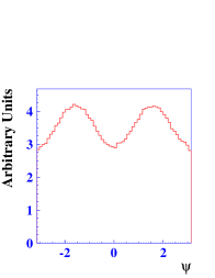
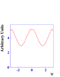
e1)	e2)	e3)

Figure 5: Simulated angular distributions for the $\omega\pi$-resonances. The figures a1), b1), c1), d1), e1) correspond to the $J^{P}=0^{-}$ ($\rho_{0}^{-}$) intermediate state; a2), b2), c2), d2), e2) — $J^{P}=1^{-}$ ($\rho(1450)^{-}$)-state; a3), b3), c3), d3), e3) — $J^{P}=1^{+}$ ($b_{1}(1235)^{-}$)-state.

a1)	a2)	a3)
b1)	b2)	b3)

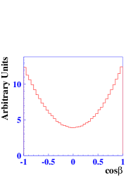
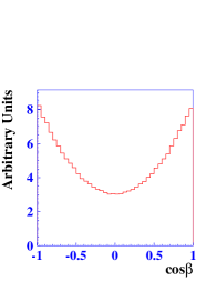
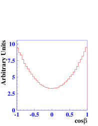
c1)	c2)	c3)
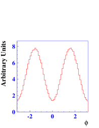
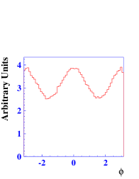
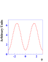
d1)	d2)	d3)
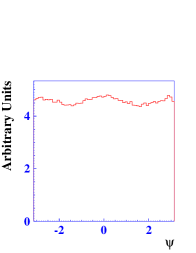
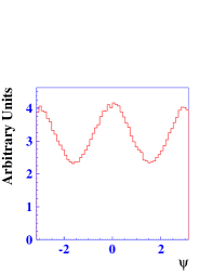
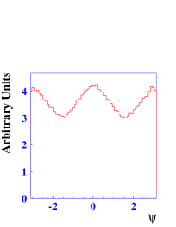
e1)	e2)	e3)

Figure 6: Simulated angular distributions for the $\omega\pi$-resonances. The figures a1), b1), c1), d1), e1) correspond to the $J^{P}=2^{+}$ ($b_{2}^{-}$) intermediate state; a2), b2), c2), d2), e2) — $2^{-}$ ($\rho_{2}^{-}$)-state; a3), b3), c3), d3), e3) — $3^{-}$ ($\rho_{3}(1690)^{-}$)-state.

a1)	a2)	a3)
b1)	b2)	b3)
c1)	c2)	c3)
d1)	d2)	d3)

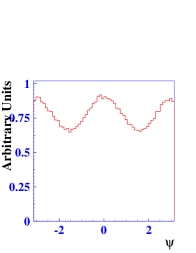
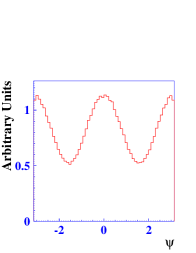
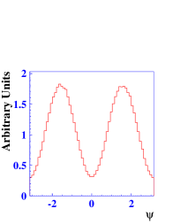
e1)	e2)	e3)

Figure 7: Simulated angular distributions for the $P$-wave $D^{**}$-resonances. The figures a1), b1), c1), d1), e1) correspond to the $J^{P}_{j_{u}}=1^{+}_{3/2}$ narrow state; a2), b2), c2), d2), e2) — $J^{P}_{j_{u}}=1^{+}_{1/2}$ broad state; a3), b3), c3), d3), e3) — $J^{P}_{j_{u}}=2^{+}_{3/2}$ narrow state.

a1)	a2)	a3)	a4)
b1)	b2)	b3)	b4)
c1)	c2)	c3)	c4)

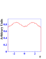
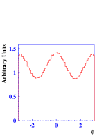
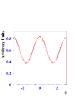
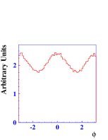
d1)	d2)	d3)	d4)
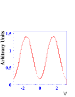
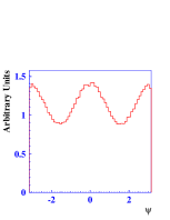
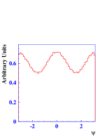
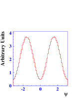
e1)	e2)	e3)	e4)

Figure 8: Simulated angular distributions for the $D$-wave $D^{**}$-resonances. The figures a1), b1), c1), d1), e1) correspond to the $J^{P}_{j_{u}}=1^{-}_{3/2}$ broad state; a2), b2), c2), d2), e2) — $J^{P}_{j_{u}}=2^{-}_{5/2}$ narrow state; a3), b3), c3), d3), e3) — $J^{p}_{j_{u}}=2^{-}_{3/2}$ broad state; a4), b4), c4), d4), e4) — $J^{P}_{j_{u}}=3^{-}_{5/2}$ narrow state.

If we consider one angular variable only, the distributions can be the same for different resonant hypotheses. Efficient separation between resonances is possible, when all angular variables are taken into account. This statement is demonstrated in Figs. 5 and 6 for the $\omega\pi$- states and in Figs. 7 and 8 for the $D^{*}\pi$-states. As mentioned above, $J^{P}=1^{+}$ $P$-wave and $J^{P}=2^{-}$ $D$-wave states are a mixture of pure states. However, for demonstration purposes we consider and show angular distributions for pure states. Moreover, we use a simple relativistic quark model of mesons to estimate constant ratios $C_{J-1}/C_{J}$ and $C_{J+1}/C_{J}$ in (3), which are responsible for relative contributions of amplitudes with different orbital momenta in the total matrix element [20]. The constant ratios for all discussed states are chosen roughly as follows: $C_{J-1}/C_{J}=3/2,\,C_{J+1}/C_{J}=2$.

For Dalitz plot analysis, interference between resonances should be taken into account. For a one-dimensional distribution, an interference term for resonances, which decay to the same final state, can cancel out after integration over other variables. However, in a real experiment such cancellation can disappear due to the nonuniform detection efficiency, so that a finite interference term can be observed. For resonances, which decay to the different final states $\omega\pi$ and $D^{*}\pi$, the interference term cannot be neglected. For demonstration purpose we show distributions between $b_{1}(1235)^{-}$ and pure $D^{0}_{1}$ as well as $\rho(1450)^{-}$ and pure $D^{{}^{\prime}0}_{1}$. However, there is possible interference between the resonant and non-resonant structures.

For simulation we use BW functions for $b_{1}(1235)^{-}$, $\rho(1450)^{-}$, $D^{0}_{1}$ and $D^{{}^{\prime}0}_{1}$. Thus, the $q^{2}$-dependent widths have to be obtained. For a $q^{2}$-dependent width of the $b_{1}$ we consider the dominant decay to the $\omega\pi$ [2]:

$$\Gamma_{b_{1}}(q^{2})\, =\,\frac{m_{b_{1}}}{\sqrt{q^{2}}}\frac{m^{4}_{b_{1}}\tilde{F}^{2}_{S}(q^{2})+b_{D}\tilde{f}^{2}_{1,2}(q^{2})\tilde{F}^{2}_{D}(q^{2})}{m^{4}_{b_{1}}+b_{D}\tilde{f}^{2}_{1,2}(m^{2}_{b_{1}})}\frac{\mathbf{p}}{\mathbf{p}_{0}}\Gamma_{b_{1}}{,}$$ (27)

where $\mathbf{p}_{0}$ is the magnitude of the $\omega$ momentum in the resonance rest frame, when $q^{2}=m^{2}_{b_{1}}$. Here, we use the fact that the experimental ratio of the amplitudes with $L=2$ and $L=0$ is about $0.3$ [2] and thus the constant $b_{D}\approx 53$. For a $q^{2}$-dependent width of the pure $D_{1}$ and pure $D^{\prime}_{1}$ we consider the decay to the $D^{*}\pi$:

$$\Gamma_{D_{1},D^{\prime}_{1}}(q^{2})\, =\,\frac{m_{D_{1},D^{\prime}_{1}}}{\sqrt{q^{2}}}\tilde{F}^{2}_{D,S}(q^{2})\frac{\mathbf{Q}}{\mathbf{Q}_{0}}\Gamma_{D_{1},D^{\prime}_{1}}{,}$$ (28)

where $\mathbf{Q}_{0}$ is the magnitude of the $D^{*}$ momentum in the resonance rest frame, when $q^{2}=m^{2}_{D_{1},D^{\prime}_{1}}$. For a $q^{2}$-dependent width of the $\rho(1450)$ we consider its decays into the $a_{1}(1260)\pi$ and $\omega\pi$ modes:

$$\Gamma_{\rho(1450)}\, =\,(1-a)\frac{m_{\rho(1450)}}{\sqrt{q^{2}}}\frac{m^{4}_{\rho(1450)}\tilde{F}^{2}_{S}(q^{2})+b_{D}\tilde{f}^{2}_{1,2}(q^{2})\tilde{F}^{2}_{D}(q^{2})}{m^{4}_{\rho(1450)}+b_{D}\tilde{f}^{2}_{1,2}(m^{2}_{\rho(1450)})}\frac{\mathbf{k}_{(a_{1})}}{\mathbf{k}_{0(a_{1})}}\Gamma_{\rho(1450)}+$$

$$+a\frac{\sqrt{q^{2}}}{m_{\rho(1450)}}\tilde{F}^{2}_{P}(q^{2})\frac{\mathbf{p}^{3}}{\mathbf{p}^{3}_{0}}\Gamma_{\rho(1450)}{,}$$ (29)

where the parameter $a=2/5$, when $\sqrt{q^{2}}>m_{a_{1}}+m_{\pi^{-}}$ [21], and $a=1$, when $\sqrt{q^{2}}\leq m_{a_{1}}+m_{\pi^{-}}$, $\mathbf{k}_{(a_{1})}$ is the momentum of the $a_{1}$ in the $\rho(1450)$ rest frame, $\mathbf{k}_{0(a_{1})}$ is the same momentum, when $\sqrt{q^{2}}=m_{\rho(1450)}$. Here, we use the fact that the experimental ratio of the amplitudes with $L=2$ and $L=0$ in the $a_{1}(1260)\to\rho\pi$ decay is about $-0.06$ [2] and accept the same value for the $\rho(1450)\to a_{1}(1260)\pi$ decay. Thus, we can estimate the constant $b_{D}\approx 182$.

Obviously, it is impossible to analyse spectra without knowledge of the relative phases in the amplitude. Thus, in Fig. 9 we show some typical distributions for different relative phases $\Delta\varphi$, such as $0$, $\pi/2$, $\pi$, $3\pi/2$ and the distribution without interference. The relative constant amplitudes between resonant matrix elements squared are chosen of one order of magnitude for the $b_{1}(1235)^{-}$ and $D^{0}_{1}$ for simplicity and one order of magnitude smaller for the $D^{{}^{\prime}0}_{1}$ than for the $\rho(1450)^{-}$ according to experiment [12]. Although small, the interference effects are not negligible.

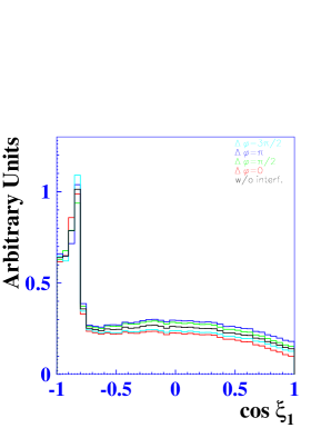
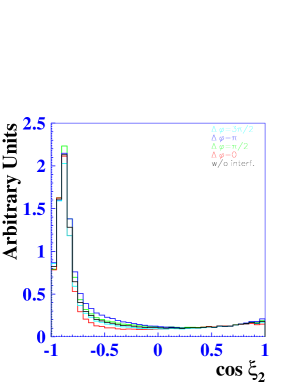
a1) $b_{1}\,D_{1}$	a2) $b_{1}\,D_{1}$
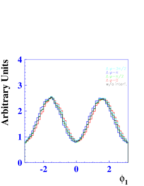
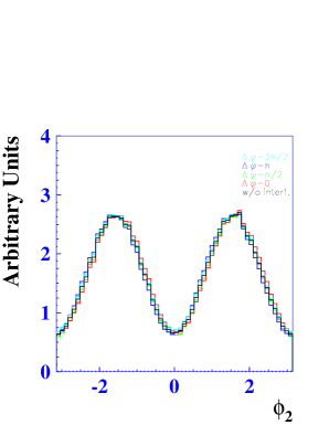
b1) $\rho^{\prime}\,D^{\prime}_{1}$	b2) $\rho^{\prime}\,D^{\prime}_{1}$

Figure 9: Demonstrative interference distributions. The figures a1), a2) correspond to the distributions over angles $\cos\xi_{1}$ and $\cos\xi_{2}$ for interference between the $b_{1}(1235)^{-}$ and pure $D^{0}_{1}$; b1), b2) correspond to the distributions over angles $\phi_{1}$ and $\phi_{2}$ for interference between the $\rho(1450)^{-}$ and pure $D^{{}^{\prime}0}_{1}$. The subscripts $1$ and $2$ correspond to the $\omega\pi$- and $D^{**}$-resonances, respectively.

7 Conclusion

We have described a model of the $\bar{B}^{0}\to D^{*+}\omega\pi^{-}$ decay, in which a total amplitude is a sum of contributions of different intermediate states. In our study we consider different resonant contributions to the matrix element, such as light $\omega\pi$-hadrons with the spin-parities of $J^{P}=0^{-},1^{\pm},2^{\pm},3^{-}$, and heavy-light hadrons, which are excitations of the $c\bar{u}$-states in $P$- and $D$-waves. All resonances are described by the relativistic Breit-Wigner factors. The resonant matrix elements are parameterized in the angular basis, which is convenient for the experimental Dalitz plot analysis and is natural from the physical point of view.

Monte-Carlo simulation based on the obtained expressions has been performed. The angular distributions obtained for the listed above intermediate states and their interference effects are demonstrated.

Appendix A Appendix

In this section we present the phase integral $W(p^{2})$ at the decay rate defined by (10). The integral

$$W(p^{2})\, =\,\pi\int_{(2m_{+})^{2}}^{(\sqrt{p^{2}}-m_{0})^{2}}dM^{2}_{0}\int_{M^{2}_{+\,min}}^{M^{2}_{+\,max}}dM^{2}_{+}\frac{\varDelta(p,P_{+},P_{0})}{p^{2}}g^{2}_{\omega\rho\pi}(p^{2})\times$$

$$\times\left|a_{3\pi}+\sum_{i=\pm,0}\frac{g_{\rho\pi\pi}}{D_{\rho^{i}}(M^{2}_{i})Z(M^{2}_{i})}\right|^{2}$$ (A1)

is a standard phase space factor for $\omega$-decay [22]. Here, the Kibble determinant $\varDelta(p,P_{+},P_{0})$, which zeros determine the phase-space boundary, is presented as follows:

$$\varDelta(p,P_{+},P_{0})\,=\,\begin{vmatrix}p^{2}&pP_{+}&pP_{0}\\ pP_{+}&m^{2}&P_{+}P_{0}\\ pP_{0}&P_{+}P_{0}&m^{2}_{0}\end{vmatrix}{,}$$

where $m$ and $m_{0}$ are the charged and neutral pions masses, respectively; the range limits of $M^{2}_{+}$ are

$$M^{2}_{+\,min}\, = \,(E^{(+-)}_{+}+E^{(+-)}_{0})^{2}-(\sqrt{E^{(+-)\,2}_{+}-m^{2}}+\sqrt{E^{(+-)\,2}_{0}-m^{2}_{0}})^{2}{,}$$

$$M^{2}_{+\,max}\, = \,(E^{(+-)}_{+}+E^{(+-)}_{0})^{2}-(\sqrt{E^{(+-)\,2}_{+}-m^{2}}-\sqrt{E^{(+-)\,2}_{0}-m^{2}_{0}})^{2}{,}$$ (A2)

where

$$E^{(+-)}_{+}\, = \,\frac{M^{2}_{0}-2m^{2}}{2M_{0}}{,}$$

$$E^{(+-)}_{0}\, = \,\frac{p^{2}-M^{2}_{0}-m^{2}_{0}}{2M_{0}}$$ (A3)

are the energies of $\pi^{+}$ and $\pi^{0}$ from $\omega$ decay in the $\pi^{+}\pi^{-}$ rest frame;

$$g_{\omega\rho\pi}(p^{2})\,=\,g_{\omega\rho\pi}(m^{2}_{\omega})\frac{1+(m_{\omega}r)^{2}}{1+(\sqrt{p^{2}}r)^{2}}$$ (A4)

is the form factor which restricts too fast growth of the width $\Gamma_{\omega}(p^{2})$ with $p^{2}$, so that $\Gamma_{\omega}(p^{2})\to\mathrm{const}$ as $p^{2}\to\infty$ (here $r$ is a hadron scale) [23]; the quantity $g_{\omega\rho\pi}(m^{2}_{\omega})\simeq 16\,\mathrm{GeV}^{-1}$ [24, 25, 26]; the $a_{3\pi}$ and $g_{\rho\pi\pi}$ amplitudes are assumed to be real constants and, thus, $a_{3\pi}=(0.01\pm 0.23\pm 0.25)\times 10^{-5}\,\mathrm{MeV}^{-2}$ [22] and $g_{\rho\pi\pi}\simeq 6$ [22, 24, 26];

$$D_{\rho^{\pm,0}}(M^{2}_{\pm,0})\,=\,M^{2}_{\pm,0}-m^{2}_{\rho^{\pm,0}}+im_{\rho{\pm,0}}\Gamma_{\rho^{\pm,0}}(M^{2}_{\pm,0}){,}$$ (A5)

where

$$M^{2}_{-}\, = \,p^{2}-M^{2}_{+}-M^{2}_{0}+m^{2}_{0}+2m^{2}{,}$$

$$\Gamma_{\rho^{\pm,0}}(M^{2}_{\pm,0})\, = \,\frac{m_{\rho^{\pm,0}}}{M_{\pm,0}}\left(\frac{k_{\pm,0}(M^{2}_{\pm,0})}{k_{\pm,0}(m^{2}_{\rho^{\pm,0}})}\right)^{3}\Gamma_{\rho^{\pm,0}}{,}$$ (A6)

$k_{i}$ is an absolute value of pion momentum in the $\pi^{+}\pi^{-}$ rest frame for $i=0$, in the $\pi^{+}\pi^{0}$ rest frame for $i=+$ and in the $\pi^{-}\pi^{0}$ rest frame for $i=-$;

$$Z(M_{\pm,0})\,=\,1-is_{1}\Phi(M_{\pm,0},\sqrt{p^{2}})$$ (A7)

is the factor taking into account the interaction of the $\rho$ and $\pi$ mesons in the final $\omega$ decay state, where the parameter $s_{1}=1\pm 0.2$ corresponds to the prediction of [27], where the specific form of the $\Phi(M_{\pm,0},\sqrt{p^{2}})$ function can be found. The couplings $g_{\omega\rho\pi}$ and $g_{\rho\pi\pi}$ are the same for $\rho^{\pm,0}$ because of isotopic invariance. As emphasized in the text, the angle $\xi$ is related to the intermediate resonance mass by a simple expression.

Finally, let us give here the $p^{2}$-dependent width of the $\omega$-meson taking into account the $3\pi$ and $\pi^{0}\gamma$ modes [2]:

$$\Gamma_{\omega}(p^{2})\,=\,\frac{W(p^{2})}{W(m^{2}_{\omega})}\mathcal{B}_{\omega\to 3\pi}\Gamma_{\omega}+\frac{m^{2}_{\omega}}{p^{2}}\frac{(p^{2}-m_{0}^{2})^{3}}{(m^{2}_{\omega}-m^{2}_{0})^{3}}\frac{g^{2}_{\omega\pi\gamma}(p^{2})}{g^{2}_{\omega\pi\gamma}(m^{2}_{\omega})}\mathcal{B}_{\omega\to\pi\gamma}\Gamma_{\omega}{.}$$ (A8)

A form factor $g_{\omega\pi\gamma}(p^{2})$ has a similar form (A4) [22] and $g_{\omega\pi\gamma}(m^{2}_{\omega})\simeq 0.7\,\mathrm{GeV}^{-1}$ [26].

References

- [1] A. F. Falk, M. E. Peskin, Phys. Rev. D 49 (1994) 3320.
- [2] Particle Data Group, K. Nakamura et al., J. Phys. G 37 (2010) 075021.
- [3] N. Isgur, M. B. Wise, Phys. Lett. B 237 (1990) 527.
- [4] M. Neubert, Phys. Rept. 245 (1994) 259.
- [5] A. Le Yaouanc, L. Oliver, O. Pene, J. C. Raynal, V. Morenas, Phys. Lett. B 520 (2001) 25.
- [6] K. Abe et al. [ Belle Collaboration ], Phys. Rev. D 69 (2004) 112002.
- [7] B. Aubert et al. [ BABAR Collaboration ], Phys. Rev. D 79 (2009) 112004.
- [8] A. Kuzmin et al. [ Belle Collaboration ], Phys. Rev. D 76 (2007) 012006.
- [9] B. Aubert et al. [ BABAR Collaboration ], Phys. Rev. Lett. 103 (2009) 051803.
- [10] N. Cabibbo, Phys. Rev. Lett. 10 (1963) 531; M. Kobayashi, T. Maskawa, Prog. Theor. Phys. 49 (1973) 652.
- [11] J. P. Alexander et al. [ CLEO Collaboration ], Phys. Rev. D 64 (2001) 092001.
- [12] B. Aubert et al. [ BABAR Collaboration ], Phys. Rev. D 74 (2006) 012001.
- [13] K. G. Wilson, Phys. Rev. 179 (1969) 1499.
- [14] A. N. Kamal, A. B. Santra, T. Uppal, R. C. Verma, Phys. Rev. D 53 (1996) 2506.
- [15] Z. Ligeti, M. E. Luke, M. B. Wise, Phys. Lett. B 507 (2001) 142.
- [16] M. Gell-Mann, D. Sharp and W. Wagner, Phys. Rev. Lett. 8 (1962) 261.
- [17] http://www.ins.cornell.edu/public/CLEO/soft/QQ
- [18] J. Blatt and V. Weisskopf, Theoretical Nuclear Physics, p.361, New York: John Wiley and Sons (1952).
- [19] F. Von Hippel, C. Quigg, Phys. Rev. D 5 (1972) 624.
- [20] M. Wirbel, B. Stech, M. Bauer, Z. Phys. C 29 (1985) 637.
- [21] R. R. Akhmetshin et al. [ CMD2 Collaboration ], Phys. Lett. B 605 (2005) 26.
- [22] M. N. Achasov et al. [SND Collaboration], Phys. Rev. D 68 (2003) 052006.
- [23] N. N. Achasov et al., Sov. J. Nucl. Phys. 54 (1991) 664.
- [24] V. M. Braun, I. E. Filyanov, Z. Phys. C 44 (1989) 157.
- [25] M. Lublinsky, Phys. Rev. D 55 (1997) 249.
- [26] J. L. Lucio-Martinez, M. Napsuciale, M. D. Scadron, V. M. Villanueva, Phys. Rev. D 61 (2000) 034013.
- [27] N. N. Achasov and A. A. Kozhevnikov, Phys. Rev. D 49 (1994) 5773.