The fixed point of the parabolic renormalization operator

1. Introduction

In a recent paper [IS], H. Inou and M. Shishikura demonstrated that the successive parabolic renormalizations ${\cal P}^{n}(f_{0})$ of the quadratic polynomial $f_{0}(z)=z+z^{2}$ converge to an analytic map $f_{*}$ defined in a neighborhood of the origin, which satisfies the fixed point equation

$${\cal P}(f_{*})=f_{*}.$$

Conjecturally, the solution of the above functional equation is unique in a suitably restricted class of maps.

In this paper we present a class of analytic maps ${{{{\mathbf{P}}}}_{0}}$ which have a maximal analytic extension to a Jordan domain, satisfying the invariance property

$${\cal P}:{{{{\mathbf{P}}}}_{0}}\to{{{{\mathbf{P}}}}_{0}}.$$

The covering properties of a map $f\in{{{{\mathbf{P}}}}_{0}}$ admit an explicit topological model. We prove that the Inou-Shishikura fixed point $f_{*}$ of ${\cal P}$ is contained in ${{{{\mathbf{P}}}}_{0}}$, and conjecture that successive renormalizations of any map $f\in{{{{\mathbf{P}}}}_{0}}$ converge to $f_{*}$.

The boundary of the maximal domain of analyticity of $f_{*}$ has a a highly degenerate geometry. It is this bad geometry that makes the study of $f_{*}$ so challenging. In contrast, consider the parabolic renormalization of critical circle maps with a parabolic fixed point on the circle, which both of the authors have studied [Lan, Ya, EY]. The corresponding renormalization fixed point also has a maximal analytic extension, whose covering properties are similar to those of $f_{*}$. The geometry of its domain of analyticity, however, is rather tame, which permits both a numerical and an analytic study.

We present a numerical method for computing the Taylor’s expansion of $f_{*}$ with a high accuracy. Our approach also allows us to compute the domain $\text{Dom}(f_{*})$, and the reader will see the first computer-generated images of it. Finally, we obtain a numerical estimate of the leading eigenvalue of $D{\cal P}|_{f_{*}}$.

2. Local dynamics of a parabolic germ

2.1. Fatou coordinates

We briefly review the local dynamics an analytic function $f$ in the vicinity of a parabolic fixed point at $0$:

$$f(z)=e^{2\pi ip/q}z+O(z^{2}).$$

We consider first the case $q=1$, that is, $f^{\prime}(0)=1$, and we write

(2.1) $$f(z)=z+az^{n+1}+O(z^{n+2}),$$

for some $n\in{\mathbb{N}}$ and $a\neq 0$. The integer $n+1$ can be recognized as the multiplicity of $0$ as the solution of $f(z)-z=0$.

A complex number $\nu$ of modulus one is called an attracting direction if the product $a\nu^{n}<0$, and a repelling direction if the same product is positive. The terminology has the following meaning:

Proposition 2.1.

Let $\{f^{k}(z)\}$ be an orbit in $\operatorname{Dom}(f)\setminus\{0\}$ which converges to the parabolic fixed point $0$. Then the sequence of unit vectors $f^{k}(z)/|f^{k}(z)|$ converges as $k\to\infty$ to one of the attracting directions.

We say in this case that the orbit converges to $p$ from the direction of $\nu$.

If $f$ has a parabolic fixed point at $0$, it admits a local inverse there, by which we mean a function $g$, defined and analytic on a neighborhood of $0$, so that $g(f(z))=z=f(g(z))$ for $z$ near enough to $0$. The germ at $0$ of a local inverse is unique, but its domain of definition typically has to be chosen. A local inverse also has a parabolic fixed point at $0$; attracting directions for $f$ are repelling for the inverse and vice versa.

Definition 2.1.

Let $\nu$ be an attracting direction for $f$. An attracting petal for $f$ (from the direction $\nu$) is a Jordan domain $P$ with closure in $\operatorname{Dom}(f)$ such that:

1. $0\in\partial P$

2. $f$ is injective on $P$;

3. $f(\overline{P}\setminus\{0\})\subset P$;

4. for any $z\in P$, the orbit $f^{k}(z)$ converges to $0$ from the direction $\nu$, and the convergence of $f^{k}$ to $0$ is uniform on $P$.

5. conversely, any orbit $f^{k}(z)$ which converges to $z$ from the direction $\nu$ is eventually in $P$.

Similarly, $U$ is a repelling petal for $f$ if it is an attracting petal for some local inverse $g$ of $f$.

Judiciously chosen petals can be organized into a Leau-Fatou Flower at $0$:

Theorem 2.2.

There exists a collection of $n$ attracting petals $P^{a}_{i}$, and $n$ repelling petals $P^{r}_{j}$ such that the following holds. Any two repelling petals do not intersect, and every repelling petal intersects exactly two attracting petals. Similar properties hold for attracting petals. The union

$$(\cup P^{a}_{i})\cup(\cup P^{r}_{j})\cup\{0\}$$

forms an open simply-connected neighborhood of $0$.

The proof of this statement relies on some changes of coordinates. First of all: Every germ of the form (2.1) can be brought into the form

(2.2) $$f(z)=z+z^{n+1}+\alpha z^{2n+1}+O(z^{3n+1})$$

in a suitable conformal local coordinate change at $0$. In fact, a straightforward induction shows the following:

Proposition 2.3 (cf. [Mil1] Problem 10-d,[BE]).

For every germ of the form (2.1) there exists a unique $\alpha\in{\mathbb{C}}$ such that for every $N\in{\mathbb{N}}$ greater that $2n+1$ there is a locally conformal change of coordinates $\psi$, with $\psi(0)=0$, such that

$$\psi\circ f\circ\psi^{-1}(z)=z+z^{n+1}+\alpha z^{2n+1}+O(z^{N}).$$

Further, there exists a formal power series $\Psi(z)=\sum_{k=1}^{\infty}p_{k}z^{k}$ which formally conjugates

$$\Psi\circ f\circ\Psi^{-1}(z)=z+z^{n+1}+\alpha z^{2n+1}.$$

Thus, the number $\alpha\in{\mathbb{C}}$ is a formal conjugacy invariant of $f$, and specifies its formal conjugacy class uniquely.

For the next few paragraphs, we will take $f$ to have the special form (2.2). The attracting directions are then the $n$th roots of $-1$. We will describe some ways of constructiong attracting petals for the attracting direction $\nu$; the adjustments necessary to deal with repelling petals are routine. The reader is reminded that (2.2) is not the general form of a mapping with a parabolic fixed point of order $n$; it has been cleaned up by making a preliminary analytic change of coordinates to eliminate some powers of $z$ in its Taylor series.

The behavior of orbits of such an $f$ near $0$ is greatly clarified by making the coordinate change

$$w=\kappa(z):=-\frac{1}{nz^{n}}.$$

We are considering a particular attracting direction, and we take $\kappa$ to be defined on the sector between the two adjacent repelling directions; it opens up this sector to the complex plane cut along the positive real axis. With its domain of definition restricted in this way, $\kappa$ is bijective, and its inverse is given by

$$\kappa^{-1}(w)=\left(-\frac{1}{nw}\right)^{1/n}$$

where the branch of the $n$-th root is the one cut along the positive real axis and taking the value $\nu$ at $-1$.

Then

$$F(w) := \kappa\circ f\circ\kappa^{-1}(w)$$

$$= -\frac{1}{n}\left(f\left(\left(-\frac{1}{nw}\right)^{\frac{1}{n}}\right)\right)^{-n}=$$

$$= -\frac{1}{n}\left(\left(-\frac{1}{nw}\right)^{\frac{1}{n}}+\left(-\frac{1}{nw}\right)^{\frac{n+1}{n}}+\alpha\left(-\frac{1}{nw}\right)^{\frac{2n+1}{n}}+O\left(\left(\frac{-1}{nw}\right)^{\frac{3n+1}{n}}\right)\right)^{-n}=$$

$$= w\cdot\left(1+\left(-\frac{1}{nw}\right)+\alpha\left(\frac{1}{nw}\right)^{2}+O\left(\frac{1}{w^{3}}\right)\right)^{-n}=$$

$$= w\cdot\left(1+\frac{1}{w}-\frac{\alpha}{n}\cdot\frac{1}{w^{2}}+\frac{n+1}{2n}\cdot\frac{1}{w^{2}}+O(\frac{1}{w^{3}})\right).$$

We thus obtain:

$$F(w)=w+1+\frac{A}{w}+O(1/w^{2})\quad\text{ as $w\to\infty$}$$

where

$$A=\frac{1}{n}\left(\frac{n+1}{2}-\alpha\right).$$

Selecting a right half-plane $H_{r}=\{\operatorname{Re}z>r\}$ for a sufficiently large $r>0$, we have

$$\operatorname{Re}F(w)>\operatorname{Re}w+1/2,\text{ and hence }F(\overline{H_{r}})\subset H_{r}.$$

The domain $\kappa^{-1}(H_{r})$ is then an attracting petal for the attracting direction $\nu$. In the case of a simple parabolic point, what we have just shown simplifies to the assertion that any disk of sufficiently small radius tangent to the imaginary axis from the left at $0$ is an attracting petal.

The petals just discussed – pullbacks of half-planes under $\kappa$ – have boundaries tangent at the origin to the directions $e^{\pm i\pi/(2n)}\nu$. For many purposes – such as the proof of Theorem 2.2 – we will need petals with strictly larger opening angle. There are many ways to construct such petals; here is one which is convenient for our purposes. Let $\pi/2<\alpha<\pi$, $R>0$, and let

(2.3) $$\Delta(\alpha,R):=\{w:-\alpha<\operatorname{Arg}(w-R)<\alpha\}$$

(i.e., $\Delta(\alpha,R)$ is the sector $\{-\alpha<\operatorname{Arg}(w)<\alpha\}$ translated right by $R$.) From

$$F(w)=w+1+O(1/w),$$

there exists a $R_{0}=R_{0}(\alpha)$ so that

(2.4) $$|\operatorname{Arg}(F(w)-w)|<\pi-\alpha\quad\text{and}\quad\operatorname{Re}(F(w))>\operatorname{Re}(w)+1/2$$

for $|w|\geq R_{0}$. If $R$ is large enough, the domain $\Delta(\alpha,R)$ does not intersect the disk $\{|w|\leq R_{0}\}$, so (2.4) holds for $w\in\Delta(\alpha,R)$. For such $R$’s, by elementary geometric considerations,

$$F\left(\overline{\Delta(\alpha,R)}\right)\subset\Delta(\alpha,R),$$

and $F^{n}(w)\underset{n\to\infty}{\longrightarrow}\infty$ for all $w\in\Delta(\alpha,R)$. Further any $\Delta(\alpha,R)$ contains a right half-plane and hence eventually contains any $F$-orbit converging to $\infty$. Finally, it can be verified that the sequence of iterates $F^{n}$ converges uniformly to $\infty$ on $\Delta(\alpha,R)$. We omit this verification; it uses simplified versions of the ideas used in the proof of Lemma 2.16. Thus, sets of the form $\kappa^{-1}\left(\Delta(\alpha,R)\right)$ are attracting petals, symmetric about the attracting direction under consideration, with tengents at the origin in directions $e^{\pm i\alpha/n}\nu$. It will be useful to have a general term for behavior for this: We will say that a petal $P$ with attracting or repelling direction $\nu$ is ample if

$$P\supset\{z:|\operatorname{Arg}(z/\nu)|<\alpha/n,|z|<r\}$$

for some $\alpha>\pi/2$ and sufficiently small $r$.

The dynamics inside a petal is described by the following:

Proposition 2.4.

Let $P$ be an attracting petal for $f$. Then there exists a conformal change of coordinates $\phi$ defined on $P$, conjugating $f(z)$ to the unit translation $T:z\mapsto z+1$.

Proof.

For a traditional proof, see e.g. [Mil1] §10. We cannot resist giving a proof based on quasiconformal surgery, which probably originated in the work of Voronin [Vor]. For definiteness, we discuss the case of an attracting petal with attracting direction $\nu$, and let

$$F(w)=w+1+O(1/w)$$

be as above. Also as above, we select a right half-plane $H_{r}$. The main step will be to prove the existence of $\phi$ for the special petal $\kappa^{-1}H_{r}$, which we provisionally denote by $P_{0}$. The case of a general petal will then follow by an easy extension argument.

As we know, $F(\overline{H_{r}})\subset H_{r},$ so let us denote $S$ the closed strip

$$S=\overline{H_{r}\setminus F(H_{r})}.$$

Setting $\SS=\{\operatorname{Re}z\in[0,1]\}$, let $h$ be any diffeomorphism

$$h:S\to\SS,$$

which on the boundary of the strip conjugates $F$ to $T$:

$$T\circ h(w)=h\circ F(w),\text{ for all }w\text{ with }\operatorname{Re}w=r.$$

We will further require that the first partial derivatives of $h$ and $h^{-1}$ be uniformly bounded in $S$. Verifying the existence a diffeomorphism with these properties is an elementary exercise which we leave to the reader.

The diffeomorphism $h$ defines a new complex structure $\mu=h_{*}\sigma_{0}$ on $\SS$, which we extend to the left half-plane $\{\operatorname{Re}z<0\}$ by

$$\mu|_{w}=(T^{n})^{*}\mu\text{ for }T^{n}(w)\in\SS.$$

Gluing together $H_{r}$ with the standard complex structure and the half-plane $\{\operatorname{Re}z<1\}$ with structure $\mu$ via the homeomorphism $h$ (which is now analytic), and using the Measurable Riemann Mapping Theorem, we obtain a new Riemann surface $X$. By the Uniformization Theorem, $X$ is conformally isomorphic either to ${\mathbb{C}}$ or to the disk. By construction, $X$ is quasiconformally isomorphic to ${\mathbb{C}}$ and therefore cannot be conformally isomorphic to the disk. We can specify a conformal isomorphism $\Phi:X\to{\mathbb{C}}$ uniquely by imposing normalization conditions $\Phi(0)=0$ and $\Phi(-1)=-1$.

The pair of maps $T|_{\{\operatorname{Re}z<0\}}$ and $F|_{H_{r}}$ induces a conformal automorphism of $X$, which we denote by $\tilde{F}$. Then $\Phi\circ\tilde{F}\circ\Phi^{-1}$ is a conformal automorphism of ${\mathbb{C}}$ with no fixed point. It is a standard fact that the only such automorphisms are translations, and our choice of normalization for $\Phi$ implies that

(2.5) $$\Phi\circ\tilde{F}\circ\Phi^{-1}\equiv T.$$

But $\tilde{F}=F$ on $H_{r}\subset X$, so we get

$$\Phi\circ F=T\circ\Phi\quad\text{on $H_{r}$.}$$

Moreover, the restriction of $\Phi$ to $H_{r}$ is analytic in the standard sense. Thus, we set $\phi:=\Phi\circ\kappa$ on $P_{0}:=\kappa^{-1}H_{r}$ and obtain

$$\phi\circ f=\phi+1\quad\text{on $P_{0}$,}$$

as desired. Since $\Phi$ is a conformal isomorphism from $X$ to ${\mathbb{C}}$, the map $\phi$ is univalent on $P_{0}$.

This proves the existence of $\phi$ on the particular petal $P_{0}$. We provisionally denote the above $\phi$, which is defined on $P_{0}$, by $\phi_{0}$. We define

$$B^{f}_{\nu}:=\{z:f^{n}(z)\to 0\quad\text{from the direction $\nu$}\}.$$

If $z_{0}\in B^{f}_{\nu}$, then $f^{n}(z_{0})\in P_{0}$ for sufficiently large $n$. If $f^{n_{0}}(z_{0})\in P_{0}$, then $(f^{n_{0}})^{-1}P_{0}$ is an open set containing $z_{0}$ and contained in $B^{f}_{\nu}$, so $B^{f}_{\nu}$ is open. Since $P_{0}$ is mapped into itself by $f$, and since

$$\phi_{0}(f(z))=\phi_{0}(z)+1\quad\text{on $P_{0}$,}$$

$\phi_{0}(f^{n}(z_{0}))-n$ takes the same value for all $n$ for which $f^{n}(z_{0})\in P_{0}$. We denote this common value by $\phi(z_{0})$, thus obtaining a function $\phi$ defined on all of $B^{f}_{\nu}$ and extending $\phi_{0}$ defined on $P_{0}\subset B^{f}_{\nu}$. Tautologically,

$$\phi(f(z))=\phi(z)+1.$$

If $f^{n_{0}}(z_{0})\in P_{0}$, then $f^{n_{0}}(z)\in P_{0}$ on a neighborhood of $z_{0}$, so $\phi(z)=\phi_{0}(f^{n_{0}}(z))-n_{0}$ on this neighborhood, which shows that the extended $\phi$ is analytic, but not necessarily univalent, on all of $B^{f}_{\nu}$.

Now let $P$ be a general attracting petal with the same attracting direction $\nu$. By definition of petal, $P\subset B^{f}_{\nu}$, so we can restrict $\phi$ to $P$, thus obtaining an analytic function satisfying

$$\phi(f(z))=\phi(z)+1\quad\text{on $P$.}$$

It remains to show that the restriction of $\phi$ to $P$ is univalent. To see this, let $z_{1}$, $z_{2}$ be points of $P$ with $\phi(z_{1})=\phi(z_{2})$. For sufficiently large $n$, $f^{n}(z_{1})$ and $f^{n}(z_{2})$ are both in $P_{0}$, so

$$\phi_{0}(f^{n}(z_{1})=\phi(z_{1})+n=\phi(z_{2})+n=\phi_{0}(f^{n}(z_{2})).$$

But, by construction, $\phi_{0}$ is univalent, so $f^{n}(z_{1})=f^{n}(z_{2})$. The argument so far works for any pair $z_{1}$, $z_{2}$ in $B^{f}_{\nu}$ with $\phi(z_{1})=\phi(z_{2})$. Now, however, we use that facts that $z_{1}$ and $z_{2}$ are both in the petal $P$, which is mapped into itself by $f$ and on which $f$ is univalent. Hence, from $f^{n}(z_{1})=f^{n}(z_{2})$ it follows that $z_{1}=z_{2}$, proving univalence of $\phi$ on $P$.

∎

We note for future reference a simple result which was proved in the course of the preceding argument:

Proposition 2.5.

Let $\nu$ be an attracting direction for $f$, $P$ be an attracting petal from the direction $\nu$, $\phi$ a univalent analytic function defined on $P$ and satisfying the function equation

$$\phi(f(z))=\phi(z)+1.$$

Then $\phi$ has a unique extension to $B^{f}_{\nu}$ satisfying this equation.

We define attracting Fatou coordinate (for the attracting petal $P$ with attracting direction $\nu$) to be a function $\phi_{A}$ defined, analytic and univalent on $P$ and satisfying

$$\phi_{A}(f(z))=\phi_{A}(z)+1\quad\text{on $P$.}$$

As we have seen, such a function extends uniquely, via the above functional equation, to all of $B_{\nu}^{f}$, and the extension restricts to an attracting Fatou coordinate on any other petal with attracting direction $\nu$. It is clear that, if $\phi_{A}$ is an attracting Fatou coordinate then so is $\phi_{A}+c$ for any constant $c$. We will see shortly that any two attracting Fatou coordinates differ only in this way.

Any attracting Fatou coordinate can be written in the form $\phi_{A}=\Phi_{A}\circ\kappa$, where $\Phi_{A}$ satisfies the functional equation

$$\Phi_{A}(F(w))=\Phi_{A}(w)+1\quad\text{(with $F=\kappa\circ f\circ\kappa^{-1}$ as above,)}$$

on an appropriate $F$-invariant domain “near infinity”. We will refer to such $\Phi_{A}$’s as Fatou coordinates at infinity.

A repelling Fatou coordinate $\phi_{R}$ for $f$ means an attracting Fatou coordinate for an analytic local inverse $g$ of $f$. If

$$f(z)=z+z^{n+1}+\ldots\text{, then }g(z)=z-z^{n+1}+\ldots,$$

which can be brought back into the standard form by conjugating with $z\mapsto-z$ ($n$ odd) or $z\mapsto i\cdot z$ ($n$ even). The above considerations then apply to define $\phi_{R}$, repelling petals, etc. We note that:

• a repelling Fatou coordinate $\phi_{R}$ satisfies the same functional equation

  $$\phi_{R}(f(z))=\phi_{R}(z)+1$$

  as does an attracting one, but the domains of definition are different, and

• the image of a repelling petal by a repelling Fatou coordinate is mapped into itself by the unit left translation $w\mapsto w-1$; the image of an ample repelling petal under a repelling Fatou coordinate contains a left half-plane.

Again, it is useful to consider also repelling Fatou coordinates at infinity: If $\phi_{R}$ is a repelling Fatou coordinate, the corresponding one at infinity is

$$\Phi_{R}(w)=\phi_{R}(\kappa^{-1}(w))$$

(but the appropriate branches of $\kappa^{-1}$ are different from the ones in the attracting case).

Our next step is to prove a crude asymptotic formula for a Fatou coordinate at infinity. It is advantageous here to deviate from what we have been doing. We consider a mapping $f$ of the form

$$f(z)=z+z^{n+1}+f_{n+2}z^{n+2}+\cdots,$$

i.e., we do not assume we have made a preliminary change of variable to eliminate, e.g., the terms $z^{j}$ for $j$ between $n+1$ and $2n+1$. We introduce $F=\kappa\circ f\circ\kappa^{-1}$ as before; this time, the behavior of $F$ near infinity is

$$F(w)=w+v(w)\quad\text{where $v(w)=1+v_{1}w^{-1/n}+v_{2}w^{-2/n}+\ldots$};$$

the series converges for sufficiently large $|w|$. Let $\Phi_{A}$ be an attracting Fatou coordinate at infinity. By what we have already proved: For any $\alpha<\pi$, there is an $R$ so that $\Phi_{A}$ extends analytically to a univalent function on the set $\{|w|>R,-\alpha<\operatorname{Arg}(w)<\alpha\}$.

Proposition 2.6.

$$\Phi_{A}^{\prime}(w)\to 1\quad\text{and}\quad\Phi_{A}(w)/w\to 1$$

uniformly as $w\to\infty$ in any sector $\{-\alpha<\operatorname{Arg}(w)<\alpha\}$ with $\alpha<\pi$. The same limits hold for $\Phi_{R}$, but with $w\to\infty$ in the opposite sector $\{-\alpha<\operatorname{Arg}(-w)<\alpha\}$

This proposition is a less-precise version of Lemma A.2.4 of [Sh], and the argument we give is the first part of Shishikura’s proof of that lemma. Shishikura carries the analysis further and is able to identify, in favorable cases, the first correction to the indicated asymptotic behaviors. We do not give his full argument here, as we will prove Theorem 2.15, which gives more precise information about the asymptotic behavior of Fatou coordinates.

Proof.

Fix $\alpha$ with $\pi/2<\alpha<\pi$, and let $\alpha<\alpha_{1}<\pi$. Take $R_{1}$ so that $\Phi_{A}$ is defined and univalent in

$$S_{1}:=\{|w|>R_{1},-\alpha_{1}<\operatorname{Arg}(w)<\alpha_{1}\}$$

and also so that $|v(w)-1|<1/4$ on $S_{1}$. For $w_{0}\in S_{1}$, denote by $\rho=\rho(w_{0})$ the distance from $w_{0}$ to the boundary of $S_{1}$. We will investigate limits as $|w_{0}|\to\infty$ in the strictly smaller sector $-\alpha<\operatorname{Arg}(w_{0})<\alpha$; then there is a constant $k>0$ so that, asymptotically, $\rho(w_{0})\geq k\cdot|w_{0}|$. In the following, we will frequently assume silently that $\rho(w_{0})$ is “large enough”. We will also use $C$ to denote a generic “universal” constant; different instances of $C$ need not denote the same constant.

For the first step, we use the Koebe Distortion Theorem: If $|w-w_{0}|<\rho-2$ – so the disk of radius 2 about $w$ is in $S_{!}$ – the mapping

$$a\mapsto\frac{\Phi_{A}(w+a)-\Phi_{A}(w)}{\Phi_{A}^{\prime}(w)}$$

is analytic and univalent on $\{|a|<2\}$ and has unit derivative at the origin. A simple rescaling of the Koebe Theorem to adapt it to the disk of radius 2 gives a universal constant $C>0$ so that

$$\left|\frac{\Phi_{A}(w+a)-\Phi_{A}(w)}{\Phi_{A}^{\prime}(w)}\right|>C^{-1}\quad\text{for $3/4<|a|<5/4$}$$

We insert $a=v(w)$ into this estimate, use $|1-v(w)|<1/4$ to ensure that $3/4<|v(w)|<5/4$, and use also the functional equation

$$\Phi_{A}(w+v(w))=\Phi_{A}(F(w))=\Phi_{A}(w)+1$$

to get

$$|\Phi^{\prime}_{A}(w)|<C\quad\text{for $|w-w_{0}|<(\rho-2)$.}$$

Applying the Cauchy estimates gives a bound

$$|\Phi^{\prime\prime}_{A}(w)|\leq\frac{C}{\rho}\quad\text{for $|w-w_{0}|<\rho/2$}$$

(with a different $C$).

Next we apply Taylor’s Formula with Integral Remainder to write

$$\Phi_{A}(w_{0}+a)=\Phi_{A}(w_{0})+a\cdot\Phi^{\prime}(w_{0})+a^{2}\cdot\int_{s=0}^{1}(1-s)\Phi^{\prime\prime}(w_{0}+s\cdot a)ds.$$

Again, we set $a=v(w_{0})$ and use $\Phi_{A}(w_{0}+v(w_{0}))=\Phi_{A}(w_{0})+1$ to get

$$1-v(w_{0})\Phi_{A}^{\prime}(w_{0})=(v(w_{0}))^{2}\int_{s=0}^{1}(1-s)\Phi^{\prime\prime}(w_{0}+s\cdot a)ds.$$

Since the estimate $|\Phi_{A}^{\prime\prime}(w)|\leq C/\rho$ holds for all $w$ appearing in the integral on the right, we get

$$|1-v(w_{0})\cdot\Phi_{A}^{\prime}(w_{0})|\leq C/\rho(w_{0}).$$

We have already remarked that $\rho(w_{0})\geq k|w_{0}|$ as $w_{0}\to\infty$ in the sector $\{-\alpha<\operatorname{Arg}(w_{0})<\alpha\}$ so

$$|\Phi_{A}^{\prime}(w_{0})-v(w_{0})^{-1}|=O(|w_{0}|^{-1})\quad\text{in that sector.}$$

This establishes the asserted convergence of $\Phi_{A}^{\prime}$; the assertion about $\Phi(w)/w$ follows by integration.

∎

Equipped with this information about the asymptotic behavior of Fatou coordinates, we can now show that the image of a Fatou coordinate is large enough. As usual, it suffices – up to insertion of some minus signs – to consider the attracting case. Let $\Phi_{A}$ be an attracting Fatou coordinate, and let $0<\alpha<\pi$. Then, for sufficiently large $R$, $\Phi_{A}$ extends analytically to a univalent function on

$$S:=\{w:|w|>R,-\alpha<\operatorname{Arg}(w)<\alpha\}$$

Proposition 2.7.

Let $0<\alpha_{0}<\alpha$. Then, for sufficiently large $R_{0}$,

$$\Phi_{A}(S)\supset S_{0}:=\{|w|<R_{0},-\alpha_{0}<\operatorname{Arg}(w)<\alpha_{0}\}.$$

Proof.

Let $w_{0}\in S_{0}$; we want to investigate solutions to the equation $\Phi_{A}(w)=w_{0}$ which we rewrite as

$$w=w_{0}+w-\Phi_{A}(w)=:\Psi_{0}(w)$$

The idea is to apply the Contraction Mapping Principle to $\Psi_{0}$, using the fact that $\Psi_{0}^{\prime}(w)=1-\Phi_{A}^{\prime}(w)$ which is small for $w$ large. To do this, we need to find a domain mapped into itself by $\Psi_{0}$ and on which $\Psi_{0}$ is contractive. Suppose we can find a $\delta>0$ so that

• $|\Psi_{0}^{\prime}(w)|<1/2$ for $|w-w_{0}|<\delta$

• $|\Psi_{0}(w_{0})-w_{0}|<\delta/2$

Then, for $|w-w_{0}|<\delta$,

$$\begin{split}|\Psi_{0}(w)-w_{0}|&\leq|\Psi_{0}(w)-\Psi_{0}(w_{0})|+|\Psi_{0}(w_{0})-w_{0}|\\ &<(1/2)\cdot|w-w_{0}|+\delta/2\leq\delta/2+\delta/2=\delta,\end{split}$$

so the disk of radius $\delta$ about $w_{0}$ will be mapped to itself, and $\Psi_{0}$ will have a unique fixed point in this disk.

We implement this strategy as follows: First of all we arrange, by making $R$ larger if necessary, that $|\Phi_{A}^{\prime}(w)-1|<1/2$ on $S$. We write

$$\epsilon:=\sin(\alpha-\alpha_{0}),$$

and we note that, by elementary geometry, $|w-w_{0}|<\epsilon\cdot w_{0}$ implies $|\operatorname{Arg}(w/w_{0})|<\alpha-\alpha_{0}$. If we further take $R_{0}\geq(1-\epsilon)^{-1}R$, then the disk of radius $\delta:=\epsilon\cdot|w_{0}|$ about $w_{0}$ is contained in $S$, for any $w_{0}\in S_{0}$. Recall that we have already arranged that $|\Psi_{0}^{\prime}|<1/2$ on $S$. Finally, we apply Proposition 2.6 to see that, by taking $R_{0}$ large enough we can arrange that

$$|\Phi_{A}(w_{0})-w_{0}|<(1/2)\cdot\epsilon\cdot|w_{0}|\quad\text{for all $w_{0}\in S_{0}$.}$$

All the element for the above contraction argument are now in place, and we can conclude that, for every $w_{0}\in S_{0}$, there is a unique $w$ with $\Phi_{A}(w)=w_{0}$ in $\{|w-w_{0}|<\epsilon|w_{0}|\}\subset S$. This proves the assertion $\Phi_{A}(S)\supset S_{0}$.

∎

It follows from this proposition that:

Proposition 2.8.

The image under $\phi_{A}$ of any ample petal of $f$ contains a right half-plane.

A similar assumption holds for ample repelling petals, but with the image under $\phi_{R}$ covering a left half-plane.

Let $P$ be an attracting petal. We define a relation on $P$ by $z_{1}\sim z_{2}$ if $z_{1}$ and $z_{2}$ are on the same orbit, that is, if either $z_{2}=f^{j}(z_{1})$ or $z_{1}=f^{j}(z_{2})$ (with $j\geq 0$.) It is easy to check that this is an equivalence relation.

Consider the quotient $P/_{\sim}$. The canonical projection $\pi:P\to P/_{\sim}$ is locally injective, and it is straightforward to verify that there is a unique way to give $P/_{\sim}$ a Riemann surface structure in such a way as to make $\pi$ analytic and therefore a local conformal isomorphism.

Let $P_{1}$ be another attracting petal contained in $P$. Since the orbit of every point $z\in P$ eventually lands in $P_{1}$, the inclusion $P_{1}\hookrightarrow P$ induces a conformal homeomorphism

$$P_{1}/\sim\underset{\simeq}{\longrightarrow}P/_{\sim}.$$

Now if $P_{2}$ is any attracting petal with the same attracting direction as $P$, the intersection $P\cap P_{2}$ is also a petal. Hence

$$P_{2}/_{\sim}\simeq P/_{\sim}\simeq(P\cap P_{2})/_{\sim}.$$

Thus, the quotient $P_{\sim}$ does not depend on the choice of the petal $P$ but only on the choice of the attracting direction $\nu$ corresponding to $P$. We will write

$$P/_{\sim}\equiv{\cal C}_{A}^{\nu}.$$

We will omit $\nu$ from the notation when the choice of the attracting direction is clear from the context (for instance, when there is only one attracting direction).

Let $\phi_{A}$ be an attracting Fatou coordinate defined on some petal $P$. It is easy to verify, using the injectivity of $\phi_{A}$ on $P$, that two points $z_{1}$ and $z_{2}$ are equivalent if and only if $\phi_{A}(z_{1})-\phi_{A}(z_{2})\in{\mathbb{Z}}$. Hence, $\phi_{A}$ defines by passage to quotients an injective mapping $\tilde{\phi}_{A}$ from ${\cal C}_{A}^{\nu}$ to ${\mathbb{C}}/{\mathbb{Z}}$. If we take $P$ to be an ample petal, then it follows from Proposition 2.8 that $\tilde{\phi}_{A}$ takes on all values in ${\mathbb{C}}/{\mathbb{Z}}$. Thus:

Proposition 2.9.

The map $\tilde{\phi}_{A}$ is a conformal isomorphism from the Riemann surface ${\cal C}_{A}^{\nu}$ to the ${\mathbb{C}}/{\mathbb{Z}}$.

In light of the preceding proposition, we will call ${\cal C}_{A}^{\nu}$ the attracting cylinder corresponding to the direction $\nu$.

The repelling cylinder ${\cal C}^{\nu}_{R}$ for $f$ is the attracting cylinder for a local inverse of $f$, fixing the origin.

If $P$ is an attracting petal, we will call the half-open domain

$$C_{A}=P\setminus fP$$

a fundamental attracting crescent, the name reflecting its shape. A fundamental repelling crescent means a fundamental attracting crescent for a local inverse of $f$.

Proposition 2.10.

For any attracting petal $P$ in the direction $\nu$, the fundamental crescent $C_{A}$ projects bijectively onto the attracting cylinder ${\cal C}^{\nu}_{A}$. More concretely: Every point of $P$ lies on a forward orbit starting in $C_{A}$, and distinct points of $C_{A}$ have disjoint forward orbits.

Proof.

From the requirement that $f^{n}$ converges uniformly to 0 on $P$ – condition (4) in of our definition of petal – it follows that no point of $P$ admits an arbitrarily long backward orbit in $P$. Thus, every point of $P$ lies on the forward orbit starting outside $P$; the first point on this orbit inside $P$ is in $C_{A}$. Let $z_{1}$, $z_{2}$ be points of $C_{A}$ whose forward orbits intersect. From the injectivity of $f$ on $P$, we have – possibly after interchanging $z_{1}$ and $z_{2}$ – $f^{n}(z_{1})=z_{2}$ for same $n\geq 0$. If $n>0$, then $z_{2}=f^{n}(z_{1})\in fP$, contradicting $z_{2}\in C_{A}$, so the only possibility left is $n=0$, i.e., $z_{1}=z_{2}$. ∎

We note the following standard fact:

Proposition 2.11.

Let $h:{\mathbb{C}}^{*}\to{\mathbb{C}}^{*}$ be an injective holomorphic map. Then either $h(z)=cz$ or $h(z)=c/z$ for a non-zero constant $c$.

Proof.

Such an $h$ is in particular an analytic function with isolated singularities at $0$ and $\infty$ (and nowhere else.) By injectivity, neither singularity can be essential, so $h$ extends to a meromorphic mapping of the Riemann sphere to itself, i.e. to a rational function. Injectivity on the sphere with two points deleted implies that this rational function has degree one, i.e., is a Möbius transformation. In particular, the extended function maps the sphere bijectively to itself, so either $h(0)=0$, in which case $h(\infty)=\infty$, or $h(0)=\infty$. In the first case, $h(z)/z$ is bounded at $\infty$ and has a removable singularity at $0$, so, by Liouville’s Theorem, $h(z)/z=c$. In the case $h(0)=\infty$, applying the above to $z\mapsto h(1/z)$ gives $h(z)=c/z$.

∎

A corollary of the above result is a uniqueness statement for Fatou coordinates:

Proposition 2.12.

Let $P$ be an attracting petal of $f$, and let $\phi_{1}$ and $\phi_{2}$ be attracting Fatou coordinates on $P$, i.e., univalent analytic functions satisfying $\phi_{i}(f(z))=\phi_{i}(z)+1$. Then $\phi_{2}(z)-\phi_{1}(z)$ is constant on $P$.

Proof.

By Proposition 2.9, $\phi_{1}$ and $\phi_{2}$ both induce conformal isomorphisms from ${\cal C}_{A}$ to ${\mathbb{C}}/{\mathbb{Z}}$. It will be more convenient to work with with the punctured plane ${\mathbb{C}}^{*}$ instead of ${\mathbb{C}}/{\mathbb{Z}}$. The function

$$\operatorname{ixp}(z):=\exp(2\pi iz)$$

induces – again by passage to quotients – a conformal isomorphism from ${\mathbb{C}}/{\mathbb{Z}}$ to $C^{*}$, so $\operatorname{ixp}\circ\phi_{1}$ and $\operatorname{ixp}\circ\phi_{2}$ both induce conformal isomorphism ${\cal C}_{A}\to{\mathbb{C}}^{*}$. Hence, the prescription

$$h:\exp(2\pi i\phi_{1}(z)))\mapsto\exp(2\pi i\phi_{2}(z))\quad\text{for all $z\in P$}$$

defines a conformal isomorphism $h:{\mathbb{C}}^{*}\to{\mathbb{C}}^{*}$. By Proposition 2.11, there are two possibilities:

1. there is a non-zero constant – which we write as $\exp(2\pi ic)$ – so that

   $$\exp(2\pi ic)\cdot\exp(2\pi i\phi_{1}(z)=\exp(2\pi i\phi_{2}(z))\quad\text{for all $z\in P$}$$

   or

2. there is a constant $c$ so that

   $$\exp(2\pi ic)\cdot\exp(-2\pi i\phi_{1}(z))=\exp(2\pi i\phi_{2}(z))\quad\text{for all $z\in P$}$$

In the first case,

$$\phi_{2}(z)-\phi_{1}(z)-c\in{\mathbb{Z}}\quad\text{for all $z\in P$.}$$

But the expression on the left is continuous, and an integer-valued continuous function on a connected set must be constant, so

$$\phi_{2}(z)=\phi_{1}(z)+c+n_{0}\quad\text{for all $z\in P$, for some $n_{0}\in{\mathbb{Z}}$}$$

which is what we wanted to prove.

In the second case, similarly,

$$\phi_{2}(z)=-\phi_{1}(z)+c+n_{0}\quad\text{for all $z\in P$,}$$

and this contradicts

$$\phi_{1}(f(z))-\phi_{1}(z)=1=\phi_{2}(f(z))-\phi_{2}(z)\quad\text{for $z\in P$,}$$

so this case is excluded. ∎

The critical values of Fatou coordinates are simply related to those of $f$:

Proposition 2.13.

Let $\phi_{A}$ be an attracting Fatou coordinate defined on $B^{f}_{\nu}$. Then critical values of $\phi_{A}$ all have the form

$$\phi_{A}(v)-n\quad\text{ with $v$ a critical value of $f$ in $B^{f}_{\nu}$ and $n\geq 1$}$$

If $f:B^{f}_{\nu}\to B^{f}_{\nu}$ is surjective, all numbers of this form are critical values.

Proof.

Iterating the functional equation for $\phi_{A}$, differentiating, and applying the chain rule gives

$$\phi_{A}^{\prime}(z)=\frac{d}{dz}\phi_{A}(f^{n}(z))=\phi_{A}^{\prime}(f^{n}(z))\prod_{j=0}^{n-1}f^{\prime}(f^{j}(z)).$$

For given $z$ and sufficiently large $n$, $f^{n}(z)$ is in an attracting petal, which implies $\phi_{A}^{\prime}(f^{n}(z))\neq 0$. Thus: $z$ is a critical point of $\phi_{A}$ if and only if there exists $j\geq 0$ such that $f^{j}(z)$ is a critical point of $f$. For such a $j$, $f^{j+1}(z)=v$ is a critical value of $f$. Since

$$\phi_{A}(z)=\phi_{A}(f^{j+1}(z))-(j+1)=\phi_{A}(v)-(j+1),$$

the assertion follows. ∎

For completeness, let us note how the situation changes if $f^{\prime}(0)$ is a $q$-th root of unity $e^{2\pi ip/q}$ with $q\neq 1$. A fixed petal for the iterate $f^{q}$ corresponds to a cycle of $q$ petals for $f$. It thus follows that $q$ divides the number $n$ of attracting/repelling directions of $0$ as a fixed point of $f^{q}$.

2.2. Asymptotic expansion of a Fatou coordinate at infinity

We will now specialize to the case $q=1$ and $n=1$. By rescaling we can then bring the coefficient of $z^{2}$ to $1$, and the normal form (2.2) becomes

(2.6) $$f(z)=z+z^{2}+\alpha z^{3}+O(z^{4}).$$

We will say in this case that $0$ is a simple parabolic fixed point of $f$. There is one attracting direction ($-1$) and one repelling direction ($+1$).

If the domain of definition $\operatorname{Dom}(f)\ni 0$ is fixed, we let $B^{f}\subset\operatorname{Dom}(f)$, as before, to denote the basin of the parabolic point at the origin. The immediate basin of $0$, which we denote $B_{0}^{f}$, is the connected component of $B^{f}$ which contains an attracting petal.

The change of variables $\kappa$ moving the parabolic point to $\infty$ becomes simply

$$\kappa(z)=-\frac{1}{z},\quad\kappa^{-1}(w)=-\frac{1}{w},$$

and we have

$$F(w)=-\left(f(-\frac{1}{w})\right)^{-1}=w+1+\frac{A}{w}+O(w^{-2}),\quad\text{with $A=1-\alpha$,}$$

and $F(w)-w$ is analytic at $\infty$.

We showed earlier (Proposition 2.6) that any attracting Fatou coordinate at infinity $\Phi_{A}$ for such an $f$ satisfies

$$\Phi_{A}(w)=w+o(w)\quad\text{as $w\to\infty$ appropriately}$$

We will prove shortly a much more precise result – an asymptotic expansion giving $\Phi_{A}$ up to corrections of order $w^{-n}$ for any $n$. Before we do this, we investigate formal solutions to the functional equation

$$\Phi(F(w))=\Phi(w)+1$$

satisfied by both attracting and repelling Fatou coordinates.

Proposition 2.14.

There is a unique sequence $b_{1},b_{2},\ldots$ of complex coefficients such that

(2.7) $$\Phi_{\text{ps}}(w)=w-A\log(w)+\sum_{j=1}^{\infty}b_{j}w^{-j}$$

satisfies

(2.8) $$\Phi_{\text{ps}}\circ F(w)=\Phi_{\text{ps}}(w)+1\quad\text{in the sense of formal power series.}$$

Furthermore, if we set

(2.9) $$\Phi_{n}(w):=w-A\log w+\sum_{j+1}^{n}b_{j}w^{-j}$$

then

(2.10) $$\Phi_{n}(F(w))-\Phi_{n}(w)-1=O(w^{-(n+2)})$$

The logarithm appearing in (2.7) – and all other logarithms in this section – are to be understood as the principal branch, i.e., the branch with a cut along the negative real axis and real values on the positive axis. Because of the logarithmic term, $\Phi_{\text{ps}}$ as written is not exactly a formal power series in $w^{-1}$. To work around this, we rewrite the equation $\Phi_{\text{ps}}\circ F=\Phi_{\text{ps}}+1$ formally as

(2.11) $$F(w)-w-1-A\log(F(w)/w)=\sum_{j=1}^{\infty}b_{j}\left(F(w)^{-j}-w^{-j}\right)$$

Since $F(w)/w$ is analytic at $\infty$ and takes the value $1$ there, $\log(F(w)/w)$ is analytic at $\infty$ and vanishes there. Furthermore, the formal identity

$$\log(F(w))-\log(w)=\log(F(w)/w)$$

holds literally on $\{-\alpha<\operatorname{Arg}(w)<\alpha,|w|>R\}$ for sufficiently large $R$, for any $\alpha<\pi$. It is equation (2.11) which we really solve.

The left-hand side of (2.11) is analytic at $\infty$, and vanishes to second order there:

$$F(w)-w-1=-Aw^{-1}+O(w^{-2})\quad\text{and}\quad\log(F(w)/w)=w^{-1}+O(w^{-2})$$

Further, $F(w)^{-j}-w^{-j}$ is analytic at infinity and vanishes to order $j+1$ there, so

$$\sum_{j=1}^{\infty}b_{j}\left(F(w)^{-j}-w^{-j}\right)$$

is indeed a formal power series in $w^{-1}$ which begins with a term in $w^{-2}$. Furthermore, the coefficient of $w^{-j-1}$ in the expression on the right in (2.11) can be written as

$$-jb_{j}+\text{a function of $b_{1}$, \ldots, $b_{j-1}$}$$

Thus, since the left-hand side of (2.11) is known, the $b_{j}$’s can be determined successively, and, by induction on $j$, they are uniquely determined. The assertion about the order of the error term $\Phi_{n}(F(w))-\Phi_{n}(w)-1$ also follows, since

$$\sum_{j=n+1}^{\infty}b_{j}\left(F(w)^{-j}-w^{-j}\right)$$

begins with a term in $w^{-(n+2)}$

Theorem 2.15.

Let $b_{1}$, $b_{2}$, …be as in Proposition 2.14, and let $\Phi_{A}$ be an attracting Fatou coordinate at infinity. Then, for any $n$,

(2.12) $$\Phi_{A}(w)=w-A\log w+C_{A}+\sum_{j=1}^{n}b_{j}w^{-j}+O(|w|^{-(n+1)})$$

uniformly as $w\to\infty$ in any sector $-\alpha<\operatorname{Arg}(w)<\alpha$ with $\alpha<\pi$

We collect the main estimates needed for the proof of Theorem 2.15 in the following lemma:

Lemma 2.16.

$$\sum_{j=0}^{\infty}|F^{j}(w)|^{-m}=O(|w|^{-(m-1)})$$

and

$$\left|(F^{j})^{\prime}(w)\right|\quad\text{is bounded uniformly in $j$}$$

both estimates holding uniformly for $w\to\infty$ in any sector $\{-\alpha<\operatorname{Arg}(w)<\alpha\}$ with $\alpha<\pi$.

Proof.

We fix an $\alpha<\pi$, and we choose an $\alpha_{1}$ with $\alpha<\alpha_{1}<\pi$; it saves trouble later if we also require that $\pi-\alpha_{1}<\pi/6$. Next we fix an $R_{0}$ large enough so that

(2.12) $$|F(w)-(w+1)|<\sin(\pi-\alpha_{1})$$

holds for $|w|>R_{0}$; then an $R_{1}$ so that the translated sector

$$\Delta(\alpha_{1},R_{1}):=\{w:-\alpha_{1}<\operatorname{Arg}(w-R_{1})<\alpha_{1}\}$$

does not intersect the disk of radius $R_{0}$ about $0$. Then (2.12) holds on $\Delta(\alpha_{1},R_{1})$, so $F$ maps $\Delta(\alpha_{1},R_{1})$ to itself; also, since $\pi-\alpha_{1}<\pi/6$, we also have – again from (2.12) –

(2.13) $$|F(w)-w-1|<\frac{1}{2}\quad\text{on $\Delta(\alpha_{1},R_{1})$.}$$

from which it follows that

(2.14) $$\operatorname{Re}(F(w)\geq\operatorname{Re}(w)+1/2\quad\text{for $w\in\Delta(\alpha_{1},R_{1})$.}$$

and also

(2.15) $$-(\pi-\alpha_{1})<\operatorname{Arg}(F(w)-w)<(\pi-\alpha_{1})$$

We will prove estimates (I) and (II) for $w\to\infty$ in $\Delta(\alpha_{1},R_{1})\cap\{-\alpha<\operatorname{Arg}(w)<\alpha\}$; this does what we want since every $w$ with $-\alpha<\operatorname{Arg}(w)<\alpha$ and sufficiently large modulus is in $\Delta(\alpha_{1},R_{1})$.

Changing notation slightly: We want then to estimate

$$\sum_{j=0}^{\infty}|F^{j}(w_{0})|^{-m},$$

for large $w_{0}$, given that

$$-\alpha_{1}<\operatorname{Arg}(w_{0}-R)<\alpha_{1}\quad\text{and}\quad-\alpha<\operatorname{Arg}(w_{0})<\alpha$$

where – crucially – $\alpha_{1}>\alpha$. We write

$$F^{j}(w_{0})=:w_{j}=:u_{j}+iv_{j}$$

In the calculation which follows, we adopt the convention that $K$ denotes some constant depending only on $\alpha$, $\alpha_{1}$ and $m$. Different instances of $K$ are not necessarily the same constant. All inequalities involving $w_{0}$ are only asserted to hold for $|w_{0}|$ large enough.

We first treat the case $-\pi/4\leq\operatorname{Arg}(w_{0})\leq\pi/4$, i.e., $|v_{0}|\leq u_{0}$. Then, by (2.14),

$$|w_{j}|\geq u_{j}\geq u_{0}+j/2,$$

so

$$\sum_{j=0}^{\infty}|w_{j}|^{-m}\leq\sum_{j=0}^{\infty}(u_{0}+j/2)^{-m}\leq Ku_{0}^{-(m-1)}\leq K|w_{0}|^{-(m-1)};$$

in the last step, we used $|v_{0}|\leq u_{0}$ to estimate $u_{0}\geq|w_{0}|/\sqrt{2}$. This proves the desired estimate in this case.

There remain the possibilities $\pi/4<\operatorname{Arg}(w_{0})<\alpha$ and $-\alpha<\operatorname{Arg}(w_{0})<-\pi/4$. The estimates in the two cases are essentially the same; for definiteness we assume that the first holds, i.e., that $w_{0}$ is in the upper half-plane. By (2.15) the $w_{j}$ are all contained in the translated sector $\{-(\pi-\alpha_{1})<w-w_{0}<+(\pi-\alpha_{1})\}$. This sector intersects the diagonal line $\{\operatorname{Re}(w)=\operatorname{Im}(w)\}$ in a segment $(\hat{w}_{-},\hat{w}_{+})$ (labeled so that $|\hat{w}_{-}|<|\hat{w}_{+}|$.) It is easy to show, either by elementary geometry or by writing explicit formulas, that

$$|\hat{w}_{-}|\geq K^{-1}|w_{0}|\quad\text{and}\quad|\hat{w}_{+}|\leq K|w_{0}|.$$

Since $u_{j+1}\geq u_{j}+1/2$, $w_{j}$, which start out above the diagonal line, will get and stay below it after finitely many steps. Let $j_{0}$ be the first index for which $w_{j}$ is below the diagonal. Using the above upper bound on $|\hat{w}_{+}|$ we get a bound

$$j_{0}\leq K|w_{0}|$$

The line segment from $w_{j_{0}-1}$ to $w_{j_{0}}$ intersects the diagonal line between $\hat{w}_{-}$ and $\hat{w}_{+}$. Since

$$|w_{j_{0}}-w_{j_{0}-1}|=|F(w_{j_{0}-1})-w_{j_{0}-1}|<3/2$$

we get

$$|w_{j_{0}}|\geq|\hat{w}_{-}|-3/2\geq K^{-1}|w_{0}|-3/2\geq K^{-1}|w_{0}|$$

By the first case treated

(2.16) $$\sum_{j=j_{0}}^{\infty}|w_{j}|^{-m}\leq K|w_{j_{0}}|^{-(m-1)}|\leq K|w_{0}|^{-(m-1)}$$

All the $w_{j}$ lie above (or on) the line through $w_{0}$ with direction $\alpha_{1}-\pi$ (and the origin lies below this line.) Using $\operatorname{Arg}(w_{0})<\alpha<\alpha_{1}$, the distance from this line to the origin satisfies a lower bound $K^{-1}|w_{0}|$. Hence each $|w_{j}|\geq K^{-1}|w_{0}|$. Since $j_{0}\leq K|w_{0}|$,

$$\sum_{j=0}^{j_{0}-1}|w_{j}|^{-m}\leq j_{0}\cdot\left(K^{-1}|w_{0}|\right)^{-m}\leq(K|w_{0}|)\cdot(K^{m}|w_{0}|^{-m})\leq K|w_{0}|^{-(m-1)}$$

Combining this estimate on the sum of the first $j_{0}$ terms with the estimate (2.16) on the sum of the rest gives

$$\sum_{j=0}^{\infty}|F^{j}(w_{0})|^{-m}\leq K|w_{0}|^{-(m-1)}$$

(for sufficiently large $|w_{0}|$), so (I) is established. (II) follows easily from (I) together with the estimate

$$F^{\prime}(w)=1+O(|w|^{-2}),$$

the chain rule, and standard manipulations for reducing estimates on products to estimates on sums.

∎

Proof of Theorem 2.15.

Let $\pi/2<\alpha<\pi$. By an argument already used several times, we can choose $R$ sufficiently large so that

$$|F(w)-w-1|<\sin(\pi-\alpha)\text{ and }\operatorname{Re}(F(w)>\operatorname{Re}{w}+1/2$$

for all $w\in\Delta(\alpha,R):=\{-\alpha<\operatorname{Arg}(w-R)<\alpha\}$ As usual, it follows from the first of these inequalities that $F(\overline{\Delta(\alpha,R)})\subset\Delta(\alpha,R)$. We are going to prove

$$\Phi_{A}(w)=\Phi_{n}(w)+O(|w|^{-(n+1)})\quad\text{as $w\to\infty$ in $\Delta(\alpha,R)$}$$

(where $\Phi_{n}$ is defined by (2.8)); this assertion for all $\alpha$ implies the assertion of the theorem for all $\alpha$.

We set

$$c_{n}(w):=\Phi_{A}(w)-\Phi_{n}(w)\quad\text{and}\quad u_{n}(w):=\Phi_{n}\circ F(w)-\Phi_{n}(w)-1.$$

By Proposition 2.14, $u_{n}$ is analytic at infinity with

(2.17) $$u_{n}(w)=d_{n+2}w^{-(n+2)}+\cdots.$$

A simple calculation gives

$$c_{n}\circ F(w)=c_{n}(w)-u_{n}(w);$$

iterating gives

$$c_{n}\circ F^{k}(w)=c_{n}(w)-\displaystyle\sum_{j=0}^{k-1}u_{n}(F^{j}(w));$$

reorganizing and differentiating gives

(2.18) $$c_{n}^{\prime}(w)=\sum_{j=0}^{k-1}u_{n}^{\prime}(F^{j}(w))\cdot(F^{j})^{\prime}(w)+c_{n}^{\prime}(F^{k}(w))\cdot(F^{k})^{\prime}(w).$$

By differentiating (2.17)

$$u_{n}^{\prime}(w)=O(|w|^{-(n+3)})\text{ as }w\to\infty,$$

so, by Lemma 2.16,

$$\sum_{j=0}^{\infty}\left|u_{n}^{\prime}(F^{j}(w))\cdot(F^{j})^{\prime}(w)\right|<\infty$$

By Proposition 2.6

$$\Phi_{A}^{\prime}(w)\to 1\quad\text{as $\operatorname{Re}(w)\to+\infty$},$$

and the same is true for $\Phi_{n}$ by an elementary calculation; hence

$$c^{\prime}_{n}(w)\to 0\quad\text{as $\operatorname{Re}(w)\to+\infty$}.$$

Thus, we can let $k\to\infty$ in (2.18) to get

$$c_{n}^{\prime}(w)=\sum_{j=0}^{\infty}u_{n}^{\prime}(F^{j}(w))\cdot(F^{j})^{\prime}(w)$$

Applying both parts of Lemma 2.16 to this representation,

(2.19) $$|c_{n}^{\prime}(w)|\leq\operatorname{const}|w|^{-(n+2)}$$

for all $w\in\Delta(\alpha,R)$. It follows from this estimate that the limit

$$\lim_{u\to\infty}c_{n}(u+iv)$$

exists and is independent of $v$. We denote this limit by $C_{A}$. Then

$$c_{n}(u+iv)=C_{A}-\int_{u}^{\infty}c_{n}^{\prime}(\sigma+iv)d\sigma,$$

so by integrating (2.19) we get

$$|c_{n}(w)-C_{A}|\leq\operatorname{const}|w|^{-(n+1)}$$

for all $w\in\Delta(\alpha,R)$, which is what we set out to prove.

∎

We insert here a simple remark which we will want to refer to repeatedly. We say that an analytic function $f:U\to{\mathbb{C}}$ is real-symmetric if the Taylor coefficients of $f$ are real at some point $x\in U\cap{\mathbb{R}}$. Note, that we do not require that $U$ itself is a real-symmetric domain. Similarly, if $x$ is a point in ${\mathbb{R}}$, we say that an analytic germ $f(z)$ at $x$ is real-symmetric if its coefficients are real.

Proposition 2.17.

Let $f$ be a real-symmetric analytic germ of the form (2.6), and let $\phi_{A}$ be an attracting Fatou coordinate for $f$. Then there is a pure imaginary constant $c$ so that

$$\overline{\phi_{A}(z)}=\phi_{A}(\overline{z})+c\quad\text{on $B^{f}_{0}$.}$$

Furthermore, the coefficients $A$, $b_{1}$, $b_{2}$, …of Theorem 2.15 are real.

Similar assertions hold for a repelling Fatou coordinate.

Proof.

Let $P$ be a small attracting petal invariant under complex conjugation (e.g., a small disk tangent to the imaginary axis at the origin.) Since $f$ commutes with complex conjugation,

$$z\mapsto\overline{\phi_{A}(\overline{z})}$$

is another univalent analytic function defined on $P$ and satisfying the usual functional equation $\phi(f(z))=\phi(z)+1$. By uniqueness up to an additive constant of the Fatou coordinate (Proposition 2.12), there is a constant $c$ so that

$$\overline{\phi_{A}(\overline{z})}=\phi_{A}(z)+c\quad\text{on $P$.}$$

In the usual way, this identity extends to all of $B^{f}_{0}$ by repeated application of the functional equation. Applying the identity at any real point $x$ shows that $c$ is pure imaginary. We omit the proofs of the other assertions, which are even simpler. ∎

2.3. A note on resurgent properties of the asymptotic expansion of the Fatou coordinates

Let us briefly mention a very different approach to the construction of the asymptotic series (2.12) originating in the works of J. Écalle [Ec].

Recall (see e.g. [Ram]) that a formal power series $\sum_{m=1}^{\infty}a_{m}x^{-m}$ is of Gevrey order $k$ if

$$|a_{m}|<CA^{n}(n!)^{\frac{1}{k}}\text{ for some choice of positive constants }C,A.$$

Consider the asymptotic expansion (2.7) for the Fatou coordinates, and denote

$$\nu_{*}(w)\equiv\sum_{j=1}^{\infty}b_{j}w^{-j}\text{, so that }\Phi_{\text{ps}}(w)=w-A\log(w)+\nu_{*}(w).$$

As was shown by Écalle for the case $A=0$ [Ec] and A. Dudko and D. Sauzin in the general case [DS]:

Theorem 2.18.

The asymptotic series $\nu_{*}=\sum_{j=1}^{\infty}b_{j}w^{-j}$ is of Gevrey order $1$.

Theorem 5.1 is a part of Écalle’s theory of resurgence as applied specifically to Fatou coordinates (see [Sau] for an account). Recall, that the Borel transform of a formal power series

$$h_{*}=\sum_{m=1}^{\infty}a_{m}x^{-m}$$

consists in applying the termwise inverse Laplace transform:

$$a_{m}x^{-m}\mapsto\frac{a_{m}\zeta^{m-1}}{(m-1)!}.$$

In the case when the formal power series is of Gevrey order $1$, this yields a series

$$\sum_{m=1}^{\infty}\frac{a_{m}\zeta^{m-1}}{(m-1)!},$$

which converges to an analytic function $\hat{h}(\zeta)$ in a neighborhood of the origin.

The following theorem describes the phenomenon of resurgence associated with the asymptotic series $\nu_{*}$, discovered by Écalle [Ec]. Écalle presented the proof for the case when $A=0$, and so the logarithmic term is absent in (2.7), and outlined an approach to it in the general case. An independent proof in the general case was recently given by A. Dudko and D. Sauzin [DS]:

Theorem 2.19.

The Borel transform $\hat{\nu}$ of the formal power series $\nu_{*}$ analytically extends from the neighborhood of the origin along every path which avoids the points $2\pi i{\mathbb{Z}}^{*}$. Furthermore, let $S_{\theta,\epsilon}$ be any sector

$$S_{\theta,\epsilon}=\{|Arg(\zeta)-\theta|<\epsilon\}\text{ such that }\overline{S_{\theta,\epsilon}}\cap\{2\pi i{\mathbb{Z}}^{*}\}=\emptyset,$$

and let $\gamma$ be any path as above which eventually lies in $S_{\theta,eps}$ (see Figure 1). Denote $\hat{\nu}^{\gamma}$ the analytic continuation along $\gamma$. Then $\hat{\nu}^{\gamma}$ is a function of exponential type:

$$|\hat{h}^{\gamma}(\zeta)|<C\exp(D|\zeta|),$$

where the constant $C$ and $D$ depend only on $\theta$ and $\epsilon$. In particular, $\hat{h}$ has an analytic continuation $\hat{h}^{+}$ to the right half plane $\{\operatorname{Re}\zeta>0\}$ and an analytic continuation $\hat{h}^{-}$ to the left half plane $\{\operatorname{Re}\zeta<0\}$.

Figure 1. An analytic continuation along a path $\gamma$ has an exponential type in a sector $S_{\theta,\epsilon}$ whose closure does not contain any of the points $2\pi i{\mathbb{Z}}^{*}$.

Consider the standard Laplace transforms

$${\cal L}^{+}(w)=\int_{0}^{\infty}e^{-w\zeta}\hat{h}(\zeta)d\zeta\text{ and }{\cal L}^{-}(w)=\int_{-\infty}^{0}e^{-w\zeta}\hat{h}(\zeta)d\zeta.$$

Note that

$$\nu^{+}\equiv{\cal L}^{+}\hat{\nu}^{+}\text{ and }\nu^{-}\equiv{\cal L}^{-}\hat{\nu}^{-}$$

are defined for $\operatorname{Re}w$ sufficiently large. The resurgent properties of $\nu_{*}$ are completed by the following refinement of Theorem 2.15:

Theorem 2.20.

[DS] The analytic functions

$$\Phi_{A}(w)=w-A\log w+\nu^{+}(w)\text{ and }\Phi_{R}(w)=w-A\log w+\nu^{-}(w).$$

Furthermore, let $\alpha<\pi/2$. Then there exist positive constants $B=B(\alpha)$, $C=C(\alpha)$ such that

$$\left|\Phi_{A}(w)-\left(w-A\log w+\sum_{j=1}^{n}b_{j}w^{-j}\right)\right|<C^{n+1}(n+1)!|w|^{-(n+1)}$$

uniformly in a sector $\{|\text{Arg}(w)|<\pi/2+\alpha\text{ and }|w|>B\}$, and similarly for $\Phi_{R}$.

Thus $\nu_{*}$ is a Gevrey asymptotic series of order $1$. It follows from Theorem 2.20 and a Stirling formula estimate that the first $n$ terms of the asymptotic series $\nu_{*}$ are useful for numerically estimating the Fatou coordinates for $|w|>\text{const}\cdot n$.

The values of the constants in Theorem 2.20 can be estimated explicitly. Dudko [Du] shows the following. Let us write

$$F(w)=w+1+a(w),\text{ where }a(w)=Aw^{-1}+O(w^{-2}),$$

and introduce functions

$$b(w)=a(w-1)=\sum_{k=1}^{\infty}c_{k}w^{-k},\text{ and }$$

$$m(w)=-A\log\left(\frac{1+w^{-1}b(w)}{1-w^{-1}}\right)+b(w)=\sum_{k=1}^{\infty}d_{k}w^{-k}.$$

Let $C_{0},\beta>0$ be such that for all $k\in{\mathbb{N}}$

$$|c_{k}|\leq C_{0}\beta^{k-1}\text{ and }|d_{k}|\leq C_{0}\beta^{k-1}.$$

Finally, let $S$ be such that $|\hat{\nu}(\zeta)|\leq S$ for $|\zeta|\leq 2$. Set

$$B=\frac{(\beta_{0}+\frac{C_{0}}{\cos\alpha})(\frac{\alpha}{8}+1)+1}{\sin\frac{\alpha}{8}}.$$

Then for all $n\in{\mathbb{N}}$

$$\left|\Phi_{A}(w)-\left(w-A\log w+\sum_{j=1}^{n}b_{j}w^{-j}\right)\right|<\left(S+\frac{C_{0}}{\cos\alpha}\left(\frac{8}{\alpha}\right)^{n+1}\right)(n+1)!|w|^{-(n+1)}$$

uniformly in a sector $\{|\text{Arg}(w)|<\pi/2+\alpha\text{ and }|w|>B\}$, and similarly for $\Phi_{R}$.

2.4. Écalle-Voronin invariants and definition of parabolic renormalization.

The Riemann surface ${\mathbb{C}}/{\mathbb{Z}}$ has two punctures at the upper end ($\operatorname{Im}z\to+\infty$), and at the lower end ($\operatorname{Im}z\to-\infty$). Filling them with points $\oplus$ and $\ominus$ respectively, we obtain the Riemann sphere. The mapping

$$\operatorname{ixp}(z)\equiv\exp(2\pi iz),$$

conformally transforms ${\mathbb{C}}/{\mathbb{Z}}\mapsto{\mathbb{C}}^{*}$, sending $\oplus\to 0$ and $\ominus\to\infty$.

Consider a germ $f$ with a simple parabolic fixed point at $0$, normalized as in (2.6). Let $P_{A}$ and $P_{R}$ be a pair of ample petals for $f$, and denote $f^{-1}$ the local branch of the inverse which fixes the origin. Note that $f^{-1}$ extends univalently to $P_{R}\cup f(P_{A})$. Fix a choice of the Fatou coordinates $\phi_{A}$ and $\phi_{R}$.

The forward orbits originating in $P_{A}$ are parametrized by points in the attracting cylinder ${\cal C}_{A}$. Similarly, $f^{-1}$-orbits in $P_{R}$ are parametrized by points in ${\cal C}_{R}$. By the definition of an ample petal, $P_{A}\cap P_{R}\neq\emptyset$. Let $z$ be any point in the intersection of the petals. It is trivial to see that the correspondence

$$\tilde{\phi}_{R}(z)\mapsto\tilde{\phi}_{A}(z)$$

defines a mapping from a subset of ${\cal C}_{R}$ to ${\cal C}_{A}$. We denote this mapping by $h$. It is more convenient for us to pass to ${\mathbb{C}}^{*}$ from ${\mathbb{C}}/{\mathbb{Z}}$ via the exponential, and consider the mapping ${\mathbf{h}}$ formally defined as

(2.20) $${\mathbf{h}}=(\operatorname{ixp}\circ\phi_{A})\circ(\operatorname{ixp}\circ\phi_{R})^{-1}.$$

We note:

Lemma 2.21.

The mapping ${\mathbf{h}}$ is analytic.

Furthermore,

Lemma 2.22.

The domain of definition of ${\mathbf{h}}$ contains a punctured neighborhood of $0$, and a punctured neighborhood at infinity. The singularities of ${\mathbf{h}}$ at $0$ is removable, the analytic extension taking the value $0$ at $0$. Similarly, ${\mathbf{h}}$ has a pole at $\infty$.

Proof.

By local theory, $P_{A}\cap P_{R}$ contains the (upward-facing) circular sector $\{w:0<|w|<r,\pi/2-\delta<\operatorname{Arg}(w)<\pi/2+\delta\}$ for sufficiently small $r$, for any $\delta<\pi/2$. By Proposition 2.7 and the crude asymptotic estimate $\phi_{R}(z)\approx-1/z$ as $z\to 0$ staying away from the positive real axis (Proposition 2.6), it follows that the image under $\phi_{R}$ of this sector contains the upper half-strip

(2.21) $$\phi_{R}(P_{A}\cap P_{R})\supset\{x+iy:0\leq x\leq 1,y>R\}$$

for sufficiently large $R$, so the domain of definition of ${\mathbf{h}}$ contains a punctured neighborhood

$$\{z:0<|z|<\exp(-2\pi R).$$

By Proposition 2.6) the infimum of $\operatorname{Im}(\phi_{A}(x+iy))$ over the strip on the right of (2.21) goes to $+\infty$ as $R\to\infty$, so ${\mathbf{h}}(z)\to 0$ as $z\to 0$, as claimed. The proofs for the assertions about $\infty$ are similar. ∎

Let us analytically continue ${\mathbf{h}}$ to the origin and to infinity. We denote $h^{+}(z)$ the analytic germ of ${\mathbf{h}}$ at $0$, and $h^{-}(z)$ the analytic germ at $\infty$. When necessary to emphasize the dependence on the germ $f$ we will write ${\mathbf{h}}_{f}$ and $h^{\pm}_{f}$.

It is easy to see that:

Proposition 2.23.

The germs $h^{+}$, $h^{-}$ do not depend on the choice of the petals $P_{A}$ and $P_{R}$.

By Proposition 2.12, an attracting (repelling) Fatou coordinate differs from our choice of $\phi_{A}$ ($\phi_{R}$) by an additive constant. A trivial verification shows that replacing $\phi_{A}$ by $\phi_{A}+c_{A}$ and $\phi_{R}$ by $\phi_{R}+c_{R}$ changes $h^{\pm}$ to

(2.22) $$w\mapsto\lambda_{A}h^{\pm}(\lambda_{R}^{-1}w)$$

with

(2.23) $$\lambda_{A}=\exp(2\pi ic_{A}),\quad\lambda_{R}=\exp(2\pi ic_{R}).$$

The scale change factors $\lambda_{A}$ and $\lambda_{R}$ can be given arbitrary non-zero values by the appropriate choices of $c_{R}$ and $c_{A}$.

We are going to show that the zero of $h^{+}$ at $0$ and the pole of $h^{-}$ at $\infty$ are simple. We will see this by deriving a useful explicit formula for the respective leading coefficients. To write this formula, we need to introduce some notation. Writing just the first few terms in the asymptotic approximations to the Fatou coordinates (Proposition 2.15):

(2.24) $$\begin{split}\phi_{A}(z)&=-\frac{1}{z}+A\log(-z)+C_{A}+O(z)\\ \phi_{R}(z)&=-\frac{1}{z}+A\log(z)+C_{R}+O(z)\end{split}$$

where

• $A=1-\alpha$, with $\alpha$ the coefficient of $z^{3}$ in the Taylor expansion for $f$ at $0$.

• the logarithms mean the standard branch, i.e., the branch with a cut along the negative real axis and real values on the positive real axis.

• $C_{R}$ and $C_{A}$ are complex constants (specifying the normalization of the Fatou coordinates)

• the term $O(z)$ in the first equation means a quantity which goes to zero at least as fast as $|z|$ as $z\to 0$ inside any sector of the form $\{z\neq 0:-\alpha<\operatorname{Arg}(z)<\alpha\}$ with $\alpha<\pi$ (a left-facing sector), and the $O(z)$ in the second means as $z\to 0$ in any similarly defined right-facing sector.

Proposition 2.24.

$$(h^{+})^{\prime}(0)=\exp\bigl{(}-2A\pi^{2}+2\pi i(C_{A}-C_{R})\bigr{)}$$

and

$$\lim_{z\to\infty}\frac{h^{-}(z)}{z}=\exp\bigl{(}+2A\pi^{2}+2\pi i(C_{A}-C_{R})\bigr{)}$$

In particular: $h^{+}$ has a simple zero at $0$, $h^{-}$ a simple pole at $\infty$, and

(2.25) $$(h^{+})^{\prime}(0)\cdot(h^{-})^{\prime}(\infty)=\exp(-4\pi^{2}A)$$

Proof.

To prove the formula for $(h^{+})^{\prime}(0)$, we look at points $z(t)$ of the form $it$, with $t$ small and positive; such $w$’s are in $B^{f}_{0}\cap P_{R}$ for any ample petal $P_{R}$. Inserting into (2.24) and using $\log(\pm it)=\log(t)\pm i\pi/2$:

$$\phi_{R}(z(t))=it^{-1}+A\log t+iA\pi/2+C_{R}+O(t)$$

$$\phi_{A}(z(t))=it^{-1}+A\log t-iA\pi/2+C_{A}+O(t).$$

We put $w(t):=\exp(2\pi i\phi_{R}(z(t)))$; then $h^{+}(w(t))=\exp(2\pi i\phi_{A}(z(t)))$ so

$$\frac{h^{+}(w(t))}{w(t)}=\exp(2\pi i(-iA\pi+C_{A}-C_{R}+O(t))),$$

so

$$(h^{+})^{\prime}(0)=\lim_{t\to 0^{+}}\frac{h^{+}(w(t))}{w(t)}=\exp\bigl{(}-2A\pi^{2}+2\pi i(C_{A}-C_{R})\bigr{)},$$

as asserted. The assertion about $h^{-}$ is proved by a similar calculation.

∎

Let us say that two pairs of germs at zero and infinity $(h^{+}_{1},h^{-}_{1})$ and $(h^{+}_{2},h^{-}_{2})$ are equivalent if there exist non-zero constants $\lambda_{A}$ and $\lambda_{R}$ so that

$$h^{\pm}_{2}(z)=\lambda_{A}h^{\pm}_{1}(\lambda_{R}^{-1}z).$$

In view of the following, let us call the equivalence class of the germs ${\mathbf{h}}_{f}=h^{\pm}_{f}$ the Écalle-Voronin invariant of $f$. By (2.25) the Écalle-Voronin invariant determines the formal conjugacy class of the simple parabolic germ $f$. A much stronger result is due to Voronin [Vor] (an equivalent version was formulated by Écalle [Ec]):

Theorem 2.25.

Two analytic germs $f_{1}$ and $f_{2}$ of the form (2.6) are conjugate by a local conformal change of coordinates $\varphi(z)$ with $\varphi(0)=0$ if and only if their Écalle-Voronin invariants are equal.

Sketch of proof.

The proof of the “only if” direction is very easy – essentially a diagram-chase. We assume

$$f_{1}=\varphi^{-1}\circ f_{2}\circ\varphi\quad\text{on a neighborhood of $0$,}$$

where $\varphi$ is analytic at $0$ with $\varphi(0)=0$, $\varphi^{\prime}(0)>0$. We label various objects attached to $f_{1}$ and $f_{2}$ with indices $1$ and $2$ respectively. Because the assertion concerns germs, we can cut down the domains of the various functions appearing as convenient. We set things up as follows:

• We fix a domain for $\varphi$ so that it is univalent.

• We fix a domain for $f_{2}$ contained in the image of $\varphi$, on which $f_{2}$ is univalent, and so that the image of $f_{2}$ is contained in the image of $\varphi$.

• We take for the domain of $f_{1}$ the preimage under $\varphi$ of the domain of $f_{2}$. Then the equation

  $$f_{1}=\varphi^{-1}\circ f_{2}\circ\varphi$$

  is exact, including domains.

It is then obvious that:

• $\varphi$ maps any ample petal for $f_{1}$ to an ample petal for $f_{2}$. We fix any ample repelling petal $P^{(1)}_{R}$ to use in the construction of ${\mathbf{h}}_{1}$, and we use $P^{(2)}_{R}:=\varphi P^{(1)}_{R}$ as repelling petal to construct ${\mathbf{h}}_{2}$.

• If $\phi^{(2)}_{A}$ is an attracting Fatou coordinate for $f_{2}$ defined on $B^{f_{2}}$ then $\phi^{(2)}_{A}\circ\varphi$ is an attracting Fatou coordinate for $f_{1}$, and similarly for repelling Fatou coordinates. To construct Écalle-Voronin pairs for the two mappings, we choose any attracting Fatou coordinate $\phi^{(2)}_{A}$ for $f_{2}$ and use $\phi^{(1)}_{A}:=\phi^{(2)}_{A}\circ\varphi$ for $f_{1}$ (and similarly for repelling Fatou coordinates.)

With things organized this way, an entirely mechanical verification shows that ${\mathbf{h}}_{1}$ and ${\mathbf{h}}_{2}$ are identical pairs of germs.

Conversely, assume that the Écalle-Voronin invariants of $f_{1}$ and $f_{2}$ are equal. By fixing the constants in Fatou coordinates for the two mapping appropriately, we can arrange that

(2.26) $$h_{1}^{+}=h_{2}^{+}\quad\text{and}\quad h_{1}^{-}=h_{2}^{-}$$

on neighborhoods of $0$ and $\infty$ respectively. Fix also small attracting and repelling petals, for instance,

$$P_{R}=-P_{A}=\{z:-1/z\in\Delta(\alpha,R)\},$$

with $\Delta(\alpha,R)$ as defined in (2.3), $\alpha$ some number in $(\pi/2,\pi)$, and $R$ large enough. With these choices, $P_{R}\cap P_{A}$ has only two components, an upper one contained in $U^{+}$ and a lower one contained in $U^{-}$. Then $\bigl{(}\phi^{(2)}_{A}\bigr{)}^{-1}\circ\bigl{(}\phi^{(1)}_{A}\bigr{)}$ conjugates $f_{1}$ to $f_{2}$ on $P_{A}$, and, correspondingly, $\bigl{(}\phi^{(2)}_{R}\bigr{)}^{-1}\circ\bigl{(}\phi^{(1)}_{R}\bigr{)}$ conjugates $f_{1}$ to $f_{2}$ on $P_{R}$. From (2.26) it follows – possibly after adding appropriate integers to the various Fatou coordinates – that the two conjugators agree on $P_{A}\cap P_{R}$. Putting them together, we obtain a conjugator on $P_{A}\cup P_{R}$, a punctured neighborhood of $0$. It is easy to see, using the asymtotic estimates for Fatou coordinates, that this conjugator extends analytically through $0$ with the value $0$ there.

∎

In fact, all equivalence classes of pairs of germs actually occur as Écalle-Voronin invariants:

Theorem 2.26.

Let $h^{+}$ be an analytic germ at $0$, with a simple zero there, and let $h^{-}$ be a meromorphic germ at $\infty$ with a simple pole there. Denote $\lambda^{+}=(h^{+})^{\prime}(0)$, $\lambda^{-}=(h^{-})^{\prime}(\infty)$, and let

$$\lambda^{+}\cdot\lambda^{-}=e^{-4\pi^{2}A}.$$

Then there exists a simple parabolic germ $f(z)$ at the origin of the form

$$f(z)=z+z^{2}+(1-A)z^{3}+\cdots$$

whose Écalle-Voronin invariant is the equivalence class of $(h^{+},h^{-})$.

Sketch of proof.

We follow the argument given in [BH]. Let us choose the lifts $H^{\pm}(w)$ of the germs $h^{\pm}$ via the exponential map:

$$e^{2\pi iH^{\pm}(w)}=h^{\pm}(e^{2\pi iw}).$$

For a sufficiently large value of $R>0$, the maps $H^{\pm}$ are defined in the half-planes $V^{\pm}\equiv\{\pm\operatorname{Im}w>R\}$. Denote $U^{\pm}\equiv H^{\pm}(V^{\pm})$ – these domains are invariant under the translation $w\mapsto w+1$ and contain half-planes $\{\pm\operatorname{Im}w>R^{\prime}\}$. We have

$$H^{\pm}(w)=w+\frac{1}{2\pi i}\log(\lambda^{\pm})+o(1),$$

let us select the branches of the logarithm so that $\log(\lambda^{+}\lambda^{-})=4\pi^{2}A.$ Fix $w^{\pm}\equiv H^{\pm}(R\pm iR).$ We define $V$ as the union of $V^{\pm}$ and the left half-plane $\{\operatorname{Re}(w)<-R\}$ and $U$ as the union of $U^{\pm}$ and the half-plane to the right of the line passing through $w^{+}$ and $w^{-}$. Let ${\cal V}$ denote the Riemann surface obtained by guing $V$ and $U$ via $H^{+}$, $H^{-}$ (see Figure 2). The result follows from the following claim:

Figure 2. An illustration of the proof of Theorem 2.26

Claim. For sufficiently large values of $R$ the Riemann surface ${\cal V}$ is conformally isomorphic to ${\mathbb{C}}\setminus{\mathbb{D}}$.

The proof of the claim is fairly straightforward, so we leave it to the reader. Let us show how to complete the argument assuming the claim. Let us select large enough value of $R$, and let $\chi:{\cal V}\to{\mathbb{C}}\setminus{\mathbb{D}}$ be the conformal isomorphism with $\chi^{\prime}(\infty)>0$. Denote

$$V^{\prime}=V\setminus\{-R-1\leq\operatorname{Re}(w)<-R\},$$

and let ${\cal V}^{\prime}$ be a subsurface of ${\cal V}$ obtained by replacing $V$ with $V^{\prime}$. The unit translation $w\mapsto w+1$ maps $V^{\prime}\to V$ and $U\to U$ and commutes with $H^{\pm}$. Hence it induces an analytic map $F:{\cal V}^{\prime}\to{\cal V}$. It is easy to see that

$$\hat{F}(w)\equiv\chi\circ F\circ\chi^{-1}(w)=w+1+\frac{A}{w}+o(\frac{1}{w}).$$

Indeed, the projections to $V$ and $U$ are the Fatou coordinates at infinity for $\hat{F}$, and $H^{\pm}$ are the changes of coordinates between $V$ and $U$. By construction,

$$f(z)\equiv-\frac{1}{\hat{F}(-\frac{1}{z})}$$

is an analytic germ at the origin with the desired properties.

∎

We are finally ready to define parabolic renormalization:

Definition 2.2.

We say that a parabolic germ $f(z)$ of the form (2.2) is renormalizable if for some – and hence for all – choices of normalization of $\phi_{A}$ and $\phi_{R}$, the coefficient of $z^{2}$ in the Taylor series of $h^{+}$ at $0$ does not vanish.

Then, by the rescaling formulas (2.22) and (2.23), then exist choices of the normalizations of the attracting and repelling Fatou coordinates so that the corresponding $h^{+}$ has the form

(2.27) $$h^{+}(w)=w+w^{2}+\cdots$$

i.e., so that $h^{+}$ has a normalized simple parabolic fixed point at $0$. The rescaling factors $\lambda_{A}$ and $\lambda_{R}$ which accomplish this are uniquely determined; the corresponding additive constants $c_{A}$ and $c_{R}$ are uniquely determined modulo ${\mathbb{Z}}$.

Definition 2.3.

For a renormalizable germ $f(z)$ of the form (2.6) we will call the analytic germ of the unique rescaling of $h^{+}$ with the form (2.27) the parabolic renormalization of $f$. We will use the notation ${\cal P}f$ for the parabolic renormalization.

We thus have

(2.28) $${\cal P}f=\operatorname{ixp}\circ\phi_{A}\circ(\phi_{R})^{-1}\circ\operatorname{ixp}^{-1},$$

with $\phi_{A}$, $\phi_{R}$ the appropriately normalized Fatou coordinates and with suitably selected branches of the inverses.

2.5. Analytic continuation of parabolic renormalization

Parabolic renormalization, as defined above, maps a renormalizable analytic germ $f$ at the origin of the form (2.6) to a germ ${\cal P}(f)$ of the same form. We will change the point of view now, and will talk about an analytic map $f$, defined in a domain $\operatorname{Dom}(f)\ni 0$, whose germ at $0$ is of the form (2.6). Note that we do not impose any conditions on the naturality of the domain $\operatorname{Dom}(f)$ at this point. The map $f$ may analytically extend beyond $\operatorname{Dom}(f)$, however, when considering orbits of points under $f$, we restrict ourselves only to the orbits which do not leave $\operatorname{Dom}(f)$.

As before, we denote $B^{f}\subset\operatorname{Dom}(f)$ the basin of $0$, and $B^{f}_{0}\subset B^{f}$ the immediate basin of $0$, that is, the connected component of $B^{f}$ which contains an attracting petal. Let us fix an attracting Fatou coordinate $\phi_{A}$ and extend it to all of $B^{f}$ via the functional equation. We also choose a repelling petal $P_{R}$ and fix a repelling Fatou coordinate $\phi_{R}$ on it.

We make the following simple observation:

Lemma 2.27.

Let $z_{1}\in B^{f}\cap P_{R}$ and let $z_{2}\in P_{R}$, and assume

$$\operatorname{ixp}(\phi_{R}(z_{1}))=\operatorname{ixp}(\phi_{R}(z_{2}))$$

Then $z_{2}\in B^{f}$ and

$$\operatorname{ixp}(\phi_{A}(z_{1}))=\operatorname{ixp}(\phi_{A}(z_{2}))$$

Proof.

From the assumption:

$$\phi_{R}(z_{2})-\phi_{R}(z_{1})=:m\in{\mathbb{Z}}.$$

We consider separately $m\geq 0$ and $m<0$. In the first case, $\phi_{R}(f^{-m}(z_{2}))=\phi_{R}(z_{1})$. Since $f^{-m}(z_{2})$ and $z_{1}$ are both in $P_{R}$, and since $\phi_{R}$ is univalent on $P_{R}$, $f^{-m}(z_{2})=z_{1}$, so $z_{2}=f^{m}(z_{1})$, so $z_{2}\in B^{f}$ and $\phi_{A}(z_{2})=\phi_{A}(z_{1})+m$ and the asserted equality holds.

Now suppose $m<0$, and let $p:=-m>0$. Then $\phi_{R}((f^{-p}(z_{1})=\phi_{R}(z_{2})$, so, arguing as above, $z_{1}=f^{p}(z_{2})$, so $z_{2}\in B^{f}$ so, again, the asserted equality holds.

∎

The above lemma implies:

Corollary 2.28.

The pair of analytic germs ${\mathbf{h}}$ extends to

$${\cal D}({\mathbf{h}})\equiv\{w=\operatorname{ixp}\circ\phi_{R}(z)\;|\text{ where }z\in B^{f}\cap P_{R}\}\cup\{0,\infty\}.$$

Furthermore,

Proposition 2.29.

The domain ${\cal D}(h)$ does not depend on the choice of the repelling petal $P_{R}$.

Proof.

Suppose $P^{(1)}_{R}$ is another repelling petal, and write ${\mathbf{h}}^{(1)}$ for the corresponding function. If $w\in{\cal D}({\mathbf{h}})$, then $w$ can be written as $\operatorname{ixp}\circ\phi_{R}(z)$, with $z\in B^{f}\cap P_{R}$. For large enough $n$, $f^{-n}(z)\in P^{(1)}_{R}$, and, since $f^{n}(f^{-n}(z))=z\in B^{f}$, $f^{-n}(z)\in B^{f}$. Hence $w=\operatorname{ixp}\circ\phi_{R}(f^{-n}(z))\in{\cal D}({\mathbf{h}}^{(1)})$ and

$${\mathbf{h}}^{(1)}(w)=\operatorname{ixp}\circ\phi_{A}(f^{-n}(z))=\operatorname{ixp}\circ\phi_{A}(z)={\mathbf{h}}(w).$$

This shows that ${\cal D}({\mathbf{h}})={\cal D}({\mathbf{h}}^{1})$. ∎

Since the derivative of the local inverse never vanishes, we have:

Lemma 2.30.

The only possibilities for critical values of ${\mathbf{h}}$ in ${\cal D}({\mathbf{h}})$ are the images under $\operatorname{ixp}$ of the critical values of $\phi_{A}$. More explicitly: $v$ is a critical value of ${\mathbf{h}}$ if and only if it can be written

$$v=\operatorname{ixp}\circ\phi_{A}(z_{c})$$

where $z_{c}$ is a critical point of $f$ belonging to $B^{f}$ and admitting a backward orbit converging to $0$.

We further prove:

Theorem 2.31.

Suppose $B^{f}_{0}$ is a Jordan domain, such that $\phi_{A}$ cannot be analytically continued through any point of $\partial B^{f}_{0}$. Then the pair of germs ${\mathbf{h}}=(h^{+},h^{-})$ has a maximal domain of analyticity $\operatorname{Dom}({\mathbf{h}})$, which is a union of two Jordan domains $W^{+}\ni 0$ and $W^{-}\ni\infty$. Furthermore, let $P_{R}$ be a repelling petal for $f$. Then

$$\partial\operatorname{Dom}({\mathbf{h}})\subset\operatorname{ixp}\circ\phi_{R}(\partial B_{0}^{f}\cap P_{R}).$$

Proof.

Let $P_{R}$ be a repelling petal which maps under $\phi_{R}$ to a left half-plane. After shrinking $P_{R}$ if necessary, we further assume that $f(P_{R})$ is also a petal. For purposes of this proof, $f^{-1}$ and $\phi_{R}^{-1}$ will mean the (two-sided) inverses of the respective restrictions to $P_{R}$. By local theory, $P_{R}\cup\{0\}$ contains a neighborhood of $0$ in $\partial B^{f}_{0}$. The component of $\partial B^{f}_{0}\cap(P_{R}\cup\{0\})$ containing $0$ is therefore a Jordan arc, which we denote by $\widetilde{\sigma}$. The intersection $\overline{P_{R}}\cap(\partial B^{f}_{0}\setminus\widetilde{\sigma})$ is compact and does not contain $0$, so $\operatorname{Re}(\phi_{R}(\,.\,))$ is bounded below on it. Hence, for $\beta$ sufficiently negative, the arc

$$\widetilde{\gamma}:=\phi_{R}^{-1}\{\operatorname{Re}{w}=\beta\}$$

is disjoint from $\partial B^{f}_{0}\setminus\widetilde{\sigma}$. We give the arc $\widetilde{\gamma}$ the clockwise orientation, which means that $\operatorname{Im}(\phi_{R}(\,.\,))$ goes to $+\infty$ at the beginning of $\widetilde{\gamma}$. The arc $\widetilde{\gamma}$ must intersect $B^{f}_{0}$; otherwise, it (with $0$ appended) would bound a repelling petal contained in $B^{f}_{0}$, which is impossible by local theory. Thus

$$\emptyset\neq\widetilde{\gamma}\cap\partial B^{f}_{0}\subset\widetilde{\sigma}.$$

Let $\gamma$ denote the initial segment of $\widetilde{\gamma}$ up to its first intersection with $B^{f}_{0}$, and denote the first intersection point by $z_{1}$. We have set things up so as to guarantee that $z_{1}\in\widetilde{\sigma}$. Then $f^{-1}\gamma$ is another arc in $B^{f}_{0}\cap P_{R}$, running from $0$ to $f^{-1}(z_{1})$, and disjoint from $\gamma$. Let $\sigma$ denote the subarc of $\partial B^{f}_{0}$ running from $z_{1}$ to $f^{-1}(z_{1})$ (with end-points included this time.) Then

$$\delta:=\gamma+\sigma-f^{-1}\gamma$$

(meaning: first traverse $\gamma$, then $\sigma$, then $f^{-1}\gamma$ backwards) is a Jordan curve. Since $\delta\setminus\{0\}$ is contained in the Jordan domain $P_{R}$, the domain $\Delta$ bounded by $\delta$ is also contained in $P_{R}$. Since $\overline{P_{R}}$ is contained in the petal $f(P_{R})$, the Fatou coordinate $\phi_{R}$ is analytic on $\overline{\Delta}\setminus\{0\}$, and

(2.29) $$W:=\operatorname{ixp}\circ\phi_{R}(\Delta\cup\gamma\cup f^{-1}\gamma)$$

is contained in ${\cal D}({\mathbf{h}})$. We are going to argue that $W\cup\{0\}$ is a Jordan domain, and that it is equal to $W^{+}$. The main steps are to show

1. $W$ is a connected open punctured neighborhood of $0$.

2. $\operatorname{ixp}\circ\phi_{R}$ maps $\sigma$ to a Jordan curve $\widehat{\sigma}$.

3. The boundary of $W$ is $\widehat{\sigma}\cup\{0\}$

Since $W$ is the image under $\operatorname{ixp}\circ\phi_{R}$ of a subset of $P_{R}\cap B^{f}_{0}$, $W\subset{\cal D}({\mathbf{h}})$. On the other hand, $\widehat{\sigma}$ is contained in the image of $\partial B^{f}_{0}$ and hence disjoint from $\operatorname{Dom}(f)$. By the Jordan curve theorem, ${\mathbb{C}}\setminus\widehat{\sigma}$ has exactly two connected components. As $W\cup\{0\}$ is connected, open, and disjoint from $\widehat{\sigma}$, it is contained in one of these components; we temporarily denote the containing component $U$. If $W$ were not all of $U$, then its relative boundary in $U$ would have to be non-empty, contradicting (3). Thus, $W\cup\{0\}$ is a Jordan domain. Further, $W\subset{\cal D}({\mathbf{h}})$ and $\widehat{\sigma}$ does not intersect ${\cal D}({\mathbf{h}})$, so $W$ must be a component of ${\cal D}({\mathbf{h}})$, i.e., must be $W^{+}\setminus\{0\}$.

To prove (1): By definition (2.29) is the continuous image of a connected set and so connected. The image of $\Delta\cup\gamma$ under $\phi_{R}$ contains an upper half-strip $\{u+iv:\beta-1<u\leq\beta,v>R\}$ for sufficiently large $R$, and this half-strip maps under $\operatorname{ixp}$ to a punctured disk about $0$, so $W$ is a punctured neighborhood of $0$.

To show that $W$ is open, it suffices to show that the image of $\gamma$ under $\operatorname{ixp}\circ\phi_{R}$ – which is the same as the image of $f^{-1}\gamma$ – is in the interior of $W$. This follows from the way $\operatorname{ixp}\circ\phi_{R}$ glues together the two edges. Roughly, any sufficiently small disk about a point of the image of $\gamma$ is the disjoint union of three parts, respectively the images under $\operatorname{ixp}\circ\phi_{R}$ of

• a differentiably-distorted half-disk in $\Delta$ with diameter along $\gamma$

• another differentiably-distorted half-disk in $\Delta$ with diameter along $f^{-1}\gamma$

• a subarc of $\gamma$

Thus, any such disk is contained in the interior of $W$.

To prove (2), we need

Lemma 2.32.

$ixp\circ\phi_{R}$ is injective on $\sigma\setminus\{z_{1},f^{-1}(z_{1})\}$ (that is, on $\sigma$ with its end-points deleted.)

We postpone the proof and proceed to deduce (2) from the lemma. Composing $\operatorname{ixp}\circ\phi_{R}$ with a continuous parametrization of $\sigma$ gives a continuous mapping from the parameter interval $[0,1]$ to ${\mathbb{C}}$ which is injective except for sending $0$ and $1$ to the same point. In an obvious way, this produces a continuous injective mapping of the circle ${\mathbb{T}}$ to ${\mathbb{C}}$, that is, a parametrized Jordan curve in ${\mathbb{C}}$.

To prove (3): it is nearly obvious that $\widehat{\sigma}$ and $0$ are contained in the boundary of $W$. To prove the converse: Let $w$ be a boundary point of $W$; let $(w_{n})$ be a sequence in $W$ converging to $w$; and, for each $n$, let $z_{n}$ be a point of $\Delta\cup\gamma$ with $w_{n}=\operatorname{ixp}\circ\phi_{R}(z_{n})$. By compactness of $\overline{\Delta}$, we can assume – by passing to a subsequence – that $z_{n}\to z\in\overline{\Delta}$. If $z=0$, then $z_{n}\to 0$ inside $\Delta\cup\gamma$, which implies $\operatorname{Im}(\phi_{R}(z_{n}))\to\infty$, which implies $w_{n}\to 0$, i.e., $w=0$. Otherwise, $w=\operatorname{ixp}\circ\phi_{R}(z)$. Since $w\notin W$, $z$ cannot be in $\Delta$, or in $\gamma$, or in $f^{-1}\gamma$, and we have already dealt with the possibility $z=0$, so we are left only with $z\in\sigma$, which implies $w=\operatorname{ixp}\circ\phi_{R}(z)\in\widehat{\sigma}$.

Modulo the proof of Lemma 2.32, this shows that $W^{+}$ is a Jordan domain and also gives a useful representation for $\partial{W}$ as the image under $\operatorname{ixp}\circ\phi_{R}$ of a fundamental domain for $f$ in $\partial B^{f}_{0}$. From this latter representation, it is evident that, if $\operatorname{ixp}\circ\phi_{A}$ cannot be analytically continued through $\partial B^{f}_{0}$, then $h^{+}={\mathbf{h}}|_{W^{+}}$ cannot be analytically continued through $\partial W$. Thus, all the assertions about $h^{+}$ are proved; the proofs of those about $h^{-}$ are similar.

∎

Proof of Lemma 2.32.

We use the same notation as in the proof of Proposition 2.31. Recall that $\widetilde{\sigma}$ denotes the component of $B^{f}_{0}\cap P_{R}$ which contains the parabolic point $0$. Deleting $0$ splits $\widetilde{\sigma}$ into two subarcs, which we denote by $\widetilde{\sigma}_{\pm}$; we will say later which is which. We parametrize $\widetilde{\sigma}$ as $t\mapsto\widetilde{\sigma}(t):t_{-}<t<t_{+}$, with parameter $t=0$ corresponding to the parabolic point $0$ and with $\widetilde{\sigma}_{+}$ corresponding to $t>0$. Since $f^{-1}$ maps $P_{R}$ into itself and $\widetilde{\sigma}$ into $\partial B^{f}_{0}$, it maps $\widetilde{\sigma}$ into itself. Using the parametrization, we conjugate $f^{-1}$ on $\widetilde{\sigma}$ to a one-dimensional mapping:

$$f^{-1}(\widetilde{\sigma}(t))=\widetilde{\sigma}(j(t)),$$

where $j(\,.\,)$ is a continuous injective mapping of the parameter interval into itself, with $j(0)=0$.

Claim: $j(\,.\,)$ is increasing, i.e, (loosely) $f$ is orientation-preserving on $B^{f}_{0}$.

We assume the claim for the moment. Since $f^{-n}$ converges uniformly to $0$ on $P_{R}$,

$$0<j(t)<t\quad\text{for $0<t<t_{+}$.}$$

Recall that $\widetilde{\gamma}$ is the image under $\phi_{R}^{-1}$ of an appropriate vertical line and that $\gamma$ is the initial segment of $\widetilde{\gamma}$, up to $z_{1}$, its first point of intersection with $B^{f}_{0}$. We choose the labelling of the components of $\widetilde{\sigma}\setminus\{0\}$ so that $z_{1}\in\widehat{\sigma}_{+}$. Then $f^{-1}(z_{1})$ is also in $\widetilde{\sigma}_{1}$ and – from the conjugacy to $j(\,.\,)$, the subarc of $\widetilde{\sigma}$ from $z_{1}$ to $f^{-1}(z_{1})$ with one end-point included and the other not is a fundamental domain for the action of $f^{-1}$ on $\widetilde{\sigma}_{+}$. In particular, two distinct points on this arc have disjoint $f^{-1}$ orbits and hence distinct images under $\operatorname{ixp}\circ\phi_{R}$.

It remains to prove the claim. We know that $f^{-1}$ maps $\widetilde{\sigma}$ into itself and hence maps $\widetilde{\sigma}_{+}$ either into itself, or into $\widetilde{\sigma}_{-}$. From injectivity of $f^{-1}$ on $\widetilde{\sigma}$, we will be done if we show that that the first alternative holds:

$$f^{-1}\widetilde{\sigma}_{+}\subset\widetilde{\sigma}_{+}.$$

By connectivity, this will follow if we show that $f^{-1}\widetilde{\sigma}_{+}\cap\widetilde{\sigma}_{+}$ is non-empty.

The labelling of the components of $\widetilde{\sigma}\setminus\{0\}$ is chosen by requiring that $\widetilde{\gamma}$ meets $\widetilde{\sigma}_{+}$ before $\widetilde{\sigma}_{-}$. The closed path made by following $\widetilde{\gamma}$ from 0 to its first meeting point $z_{1}$ with $\widetilde{\sigma}$, then $\widetilde{\sigma}_{+}$ back to $0$, is a Jordan curve; denote the domain it bounds by $U$. The first place $\widetilde{\sigma}_{-}$ meets $\widetilde{\gamma}$ is outside $\overline{U}$; since $\widetilde{\sigma}_{-}$ does not intersect the boundary of $U$, all of $\widetilde{\sigma}_{-}$ is outside of $U$. Thus, any continuous path in $P_{R}$ which starts in $U$ and reaches $\widetilde{\sigma}_{-}$ must intersect $\widetilde{\sigma}_{+}$ first. It is easy to see, using local theory, that $f^{-1}\gamma$ starts out in $U$. The first place where $f^{-1}\gamma$ intersects $\widetilde{\sigma}$ is $f^{-1}(z_{1})$, so

$$f^{-1}(z_{1})\in\widetilde{\sigma}_{+}\cap f^{-1}\widetilde{\sigma}_{+},$$

completing the proof.

∎

Let us introduce a model for the dynamics of a map on its immediate basin. We use the notation $B:{\mathbb{D}}\to{\mathbb{D}}$ for the quadratic Blaschke product

(2.30) $$B(z)=\frac{3z^{2}+1}{3+z^{2}}$$

We prove:

Theorem 2.33.

Let $f$ be an analytic function with a normalized simple parabolic point at the origin. Assume that the immediate basin $B_{0}^{f}$ is simply-connected, and $f:B_{0}^{f}\to B_{0}^{f}$ is a degree-2 branched covering map. Then there is a conformal isomorphism $\varphi:B_{0}^{f}\to{\mathbb{D}}$ so that

$$f=\varphi^{-1}\circ B\circ\varphi\quad\text{on $B_{0}^{f}$,}$$

where $B(z)$ is as in (2.30). In particular, any two analytic maps satisfying the conditions of the theorem are conformally conjugate on their respective $B_{0}$’s.

Proof.

For each sufficiently large $j\in{\mathbb{N}}$, let $\sigma_{j}$ denote that component of the intersection with $B^{f}_{0}$ of the circle of radius $1/j$ about $0$ which contains $-1/j$. Thus for large $j$, the arc $\sigma_{j}$ is almost the whole circle: a small closed arc near the positive real axis has been cut out. It is immediate that each $\sigma_{j}$ is a crosscut of $B^{f}_{0}$ and that $\sigma_{j}$’s for different $j$’s are disjoint (see Figure LABEL:fig-crosscut (a)). Let $N_{j}$ be the crosscut neighborhood of $\sigma_{j}$ which does not intersect $\sigma_{j-1}$. It is evident that $\sigma_{j+1}\subset N_{j}$. The diameter of $\sigma_{j}$ is at most $2/j\to 0$, hence the crosscut neighborhoods $N_{j}$ form a fundamental chain. It is clear that the impression of this fundamental chain contains $0$. Recalling that a prime end is an equivalence class of fundamental chains, we denote by $\widehat{0}$ the prime end containing the above fundamental chain.

By Riemann Mapping Theorem, there is a conformal isomorphism $\varphi$ from $B^{f}_{0}$ to ${\mathbb{D}}$ mapping the unique critical point of $f$ in $B^{f}_{0}$ to $0$. By Carathéodory theory, $\varphi$ extends to map the set of prime ends of $B^{f}_{0}$ homeomorphically to the unit circle. We can further require that the extension of $\varphi$ sends $\widehat{0}$ to $1$; with this additional condition, $\varphi$ is unique.

We use $z_{n}\underset{\text{p.e.}}{\to}\widehat{0}$ as an abbreviation for the assertion that $z_{n}$ is eventually in $N_{j}$ for each $j$. From the construction of the topology on the space of prime ends and of the Carathéodory extension, we extract the following:

Continuity at ${\mathbf{0}}$: Let $(z_{n})$ be a sequence in $B^{f}_{0}$. Then $\varphi(z_{n})\to 1$ if and only if $z_{n}\underset{\text{p.e.}}{\to}\widehat{0}$.

In view of the construction of the crosscuts $\sigma_{j}$, it might appear at first glance that the requirement that $z_{n}\underset{\text{p.e.}}{\to}\widehat{0}$ is more or less the same as the requirement that $z_{n}\to 0$. However, proving this requires more control over the structure of $\partial B^{f}_{0}$ than we have. We next develop a convenient condition which suffices to guarantee convergence of $\varphi(z_{n})$ to $1$.

Let $P_{R}$ be a repelling petal which maps under $\phi_{R}$ to a left half-plane $\{u+iv:u<\beta\}$. To give some room for maneuver, we assume that there is a larger petal $P_{R}^{\prime}$ mapping to the half-plane $\{u<\beta^{\prime}\}$ for some $\beta^{\prime}>\beta$. For the next few paragraphs, $\phi_{R}^{-1}$ will denote the inverse of the restriction of $\phi_{R}$ to $P_{R}^{\prime}$.

We next need to argue that $\operatorname{Im}(\phi_{R})$ is bounded on $P_{R}\setminus B^{f}_{0}$. More precisely, let $M$ be a positive number such that, if $z\in P_{R}$ with

$$|\operatorname{Im}(\phi_{R}(z))|\geq M,$$

then $z\in B^{f}_{0}$ (see Figure 3 (b)).

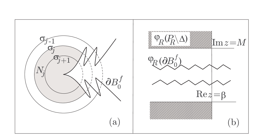
Figure 3. An illustration of the proof of Theorem 2.33

Now let $\Delta:=\{z\in P_{R}:|\operatorname{Im}(\phi_{R}(z)|\leq M\}$.

Lemma 2.34.

If $(z_{n})$ is a sequence in $B^{f}_{0}\setminus\Delta$ such that $z_{n}\to 0$, then $z_{n}\underset{\text{p.e}}{\longrightarrow}\widehat{0}$

Proof of lemma 2.34.

Recall the definition of the crosscut neighborhoods $N_{j}$ above, and let $D_{j}$ denote the open disk of radius $1/j$ about $0$. Let $\gamma_{1}$ and $\gamma_{2}$ denote the segments of the upper and lower edges of $\Delta$ which start at $0$ and extend to the first point where the edges in question meet the circle bounding of $D_{j}$.

Then $\gamma_{1}$ and $\gamma_{2}$ are crosscuts of $N_{j}$; deleting them splits $N_{j}$ into 3 subdomains, one of which is bounded by $\gamma_{1}$, $\gamma_{2}$, and a left-facing arc of the circle bounding $D_{j}$. All we want to extract from the above is that this latter domain is contained in $N_{j}$. On the other hand, elementary topological considerations, resting on the fact that the two edges of $\Delta$ are smooth arcs tangent to the positive imaginary axis at $0$, show that the domain described above is $D_{j}\setminus\Delta$ for large enough $j$. In short:

$$D_{j}\setminus\Delta\subset N_{j}\quad\text{for sufficiently large $j$.}$$

Now fix a $j$ large enough so that the above holds. If $z_{n}$ converges to $0$ staying outside of $\Delta$, it is eventually in $D_{j}\setminus\Delta$; hence, eventually in $N_{j}$. This holds for all sufficiently large $j$, so $z_{n}\underset{\text{p.e}}{\longrightarrow}\widehat{0}$, as asserted. ∎

We return to the proof of Theorem 2.33. By assumption, $f:B^{f}_{0}\to B^{f}_{0}$ is a degree-2 branched cover, and $B$ is the conjugate of $f$ on $B^{f}_{0}$ under a conformal isomorphism $\varphi:B^{f}_{0}\to{\mathbb{D}}$. Thus, $B$ is a degree-2 branched cover of ${\mathbb{D}}$ to itself. It is a standard fact – following from an easy application of the Schwarz lemma – that such a $B$ has the form

$$B(z)=e^{i\theta}\frac{z^{2}-a}{1-\overline{a}z^{2}},$$

where $a\in{\mathbb{D}}$ and $\theta\in{\mathbb{R}}$. By this formula, $B$ extends analytically to a neighborhood of the closed disk. To complete the proof, we just need to determine $\theta$ and $a$.

For any $z_{0}\in B^{f}_{0}$, $f^{n}(z_{0})$ converges to $0$ from the negative real direction, so $z_{n}$ is eventually outside $\Delta$, so, by Lemma 2.34 $z_{n}\underset{\text{p.e}}{\to}\widehat{0}$, so $\varphi(f^{n}(z_{0}))=B^{n}(\varphi(z_{0}))\to 1$, from which it follows that $1$ is a fixed point of $B$:

$$B(1)=1.$$

Since $B$ maps the unit circle to itself, preserving orientation, $B^{\prime}(1)$ is real and positive. Since the orbit $B^{n}(\varphi(z_{0}))\to 1$, it is not possible that $B^{\prime}(1)>1$.

Now specialize to $z_{0}\in B^{f}_{0}\cap P_{R}$ with $\operatorname{Im}(\phi_{R}(z_{0}))>M$. Let $f^{-1}$ denote the inverse of the restriction of $f$ to $P_{R}$. Then, for any $n\geq 0$, $f^{-n}(z_{0})\in P_{R}$ and $\operatorname{Im}(\phi_{R}(f^{-n}(z_{0}))=\operatorname{Im}(\phi_{R}(z_{0}))>M$, so $f^{-n}(z_{0})\in B^{f}_{0}\setminus\Delta$. Since $z_{0}$ is in the repelling petal $P_{R}$, $f^{-n}(z_{0})\to 0$, so, by Lemma 2.34, $y_{-n}:=\varphi(f^{-n}(z_{0}))\to 1$. The sequence $(y_{-n})$ is a backward orbit for $B$: $B(y_{-n-1})=y_{-n}$. The existence of just one backward $B$-orbit converging to the fixed point $1$ of $B$ implies

• $B^{\prime}(1)$ cannot be $<1$, so $B^{\prime}(1)$ must be equal to $1$

• $B^{\prime\prime}(1)$ cannot be non-zero; if it were, any backward orbit converging to $1$ would have to do so from the positive real direction – in particular, from outside ${\mathbb{D}}$ – whereas our sequence $y_{-n}$ is inside ${\mathbb{D}}$.

We thus have the general algebraic formula for $B(z)$ and the conditions:

$$B(1)=1,\quad B^{\prime}(1)=1,\quad B^{\prime\prime}(1)=0;$$

routine algebra then shows that $B(z)$ must be as in the statement of the theorem.

∎

3. Global theory

3.1. Basic facts about branched coverings.

We give a brief summary of relevant facts about analytic branched coverings. A more detailed exposition is found e.g. in the Appendix E of [Mil1].

For a holomorphic map $f:X\to Y$ between two Riemann surfaces a regular value is a point $y\in Y$ for which one can find an open neighborhood $U=U(y)$ such that

$$f^{-1}(U)\overset{f}{\longrightarrow}U$$

is a covering map. The complement of this set consists of the singular values of $f$, and will be denoted $\operatorname{Sing}(f)$.

By definition, $y\in Y$ is an asymptotic value of $f$ if there exists a parametrized path

$$\gamma:(0,1)\to X\text{, such that }\lim_{t\to 1-}f(\gamma(t))=y,$$

and such that $\lim_{t\to 1-}\gamma(t)$ does not exist in $X$. We will be concerned with the situation when $X$ is a proper subdomain of the Riemann sphere. In this case, the non-existence of the limit can be replaced with:

$$\gamma(t)\underset{t\to 1-}{\longrightarrow}{\partial X}.$$

We will denote $\operatorname{Asym}(f)\subset Y$ the set of all asymptotic values of $f$.

Recall that $y_{0}\in Y$ is called a critical value (or a ramified point) of $f$ if there exists $x_{0}\in X$ such that $y_{0}=f(x_{0})$, and the local degree of $f$ at $x_{0}$ is $n\geq 2$. Thus, in local coordinates, one has

$$f(x)-y_{0}=c(x-x_{0})^{n}+\cdots\text{ where }n\geq 2.$$

The point $x_{0}$ is called a critical point of $f$ (or a ramification point). We denote $\operatorname{Crit}(f)\subset X$ the set of the critical points of $f$. One then has:

Proposition 3.1.

For a holomorphic map $f:X\to Y$ between Riemann surfaces,

$$\operatorname{Sing}(f)=\overline{\operatorname{Asym}(f)\cup f(\operatorname{Crit}(f))};$$

that is, the set of the singular values of $f$ is the closure of the union of its asymptotic and critical values.

Recall that a non-constant map $g:S_{1}\to S_{2}$ between two Hausdorff topological spaces is called proper if the preimage of every compact set of $S_{2}$ is compact in $S_{1}$. It is easy to see that:

Proposition 3.2.

Let $f:X\to Y$ be a proper holomorphic map of Riemann surfaces. Let $W$ be a non-empty connected open subset of $Y$, and let $V$ be a connected component of $f^{-1}(W)$. Then $f:V\to W$ is also proper.

For a holomorphic map $f:X\to Y$ define the degree of $f$ at $y\in Y$ (denoted $\operatorname{deg}_{y}(f)$) as the possibly infinite sum of the number of preimages of $y$ in $X$, counted with multiplicity. It is not difficult to see that a proper analytic map has a well-defined local degree:

Proposition 3.3.

If $f:X\to Y$ is a proper analytic map between Riemann surfaces, and $Y$ is connected, then $\operatorname{deg}_{y}(f)$ is finite and independent of $y$ (and can be denoted as $\operatorname{deg}(f)$).

As a consequence, note:

Proposition 3.4.

If $f:X\to Y$ is a proper analytic map between Riemann surfaces, and $Y$ is connected, then $f(X)=Y$.

Proposition 3.5.

Let $g:S_{1}\to S_{2}$ be a proper continuous map between Hausdorff topological spaces which is everywhere a local homeomorphism. Then $f$ is a covering map.

In particular, putting together Proposition 3.3 and Proposition 3.5, we have

Proposition 3.6.

Let $f:X\to Y$ be a proper analytic mapping between Riemann surfaces. Let $Y$ be connected, and set $d=\operatorname{deg}(f)$. Then

$$f:X\setminus\operatorname{Crit}(f)\to Y\setminus f(\operatorname{Crit}(f))$$

is a degree $d$ covering.

In view of the above, a proper analytic map is sometimes called a branched covering of a finite degree. Generalizing to the case when local degree is infinite gives the following definition:

Definition 3.1.

A holomorphic map $f:X\to Y$ between Riemann surfaces is a branched covering if every point $y\in Y$ has a connected neighborhood $U\equiv U(y)$ such that the restriction of $f$ to each connected component of $f^{-1}(U)$ is a proper map.

As a canonical example, consider the case $X=Y=\hat{\mathbb{C}}$. Non-constant rational maps $f$ are clearly branched coverings; and every branched covering is, in fact, a rational map.

Let us formulate another general lemma which we will find useful:

Lemma 3.7.

Let $f:U\to V$ be a proper analytic map between connected subdomains of $\hat{\mathbb{C}}$. Assume that $f$ has a single critical value $v\in V$, and that $V$ is a topological disk. Then $U$ is also a topological disk, and $f$ has only one critical point $u$ in $U$, such that $f^{-1}(v)=\{u\}$.

Proof.

Set $\hat{V}\equiv V\setminus\{v\}$ and $\hat{U}\equiv f^{-1}(\hat{V})$. By Proposition 3.6, the map $f:\hat{U}\to\hat{V}$ is a covering. The domain $\hat{V}$ is homeomorphic to ${\mathbb{D}}\setminus\{0\}$. By the standard facts about coverings of ${\mathbb{D}}\setminus\{0\}$, the domain $\hat{U}$ is also homeomorphic to the punctured disk. Moreover, denoting $\eta_{\hat{V}}$ and $\eta_{\hat{U}}$ conformal homeomorphisms mapping ${\mathbb{D}}\setminus\{0\}$ to $\hat{V}$ and $\hat{U}$ respectively, we see that

$$\eta_{\hat{V}}(f(z))=\text{const}\cdot(\eta_{\hat{U}}(z))^{d}\text{ for }d\geq 2.$$

∎

3.2. Parabolic renormalization of the quadratic map.

A key example for our investigation is the quadratic polynomial

$$f_{0}(z)=z\mapsto z+z^{2}.$$

It is well known that

• The basin of attraction $B^{f_{0}}=:B_{0}$ of the parabolic point is connected.

• $f:B_{0}\to B_{0}$ is a branched cover of degree 2.

We will prove more detailed or more general versions of these assertions later – see, in particular, the proof of Theorem 3.10 – so we won’t repeat the proofs here.

By a trivial computation, $-1/2$ is a critical point of $f_{0}$; it is the only one in the finite plane, and the corresponding critical value is $-1/4$. Let $\phi_{A}$ be an attracting Fatou coordinate for $f_{0}$, defined on all of $B_{0}$. Using Proposition 2.13 and taking into account the surjectivity of $f_{0}$ on $B_{0}$, we get

Proposition 3.8.

The critical points of $\phi_{A}$ are the preimages – under iterates of $f_{0}$ – of the critical value $-1/4$:

$$\operatorname{Crit}(\phi_{A})=\cup_{n\geq 1}f_{0}^{-n}(-1/4).$$

All critical points have local degree $2$, and their images are integer translates of each other:

$$\phi_{A}(\operatorname{Crit}(\phi_{A}))=\{\phi_{A}(-1/4)-n,n\geq 1\}.$$

By standard results of complex dynamics:

(3.1) $$\overline{\text{Crit}(\phi_{A})}=\text{Crit}(\phi_{A})\cup J(f_{0}).$$

In fact (cf. [Do2]), $\phi_{A}$, mapping $B_{0}$ to ${\mathbb{C}}$, is a branched cover (but we won’t need this result.)

Our next objective is the following:

Theorem 3.9.

Let $(h^{+},h^{-})$ be an Écalle-Voronin pair for $f_{0}$ (i.e., one constructed with some choice of normalization for $\phi_{A}$ and $\phi_{R}$.) Then the germs $h^{+}$ (at 0) and $h^{-}$ (at $\infty$) have maximal analytic continuations to Jordan domains $\hat{W}^{+}$ and $\hat{W}^{-}$ (in the sphere $\hat{\mathbb{C}}$).

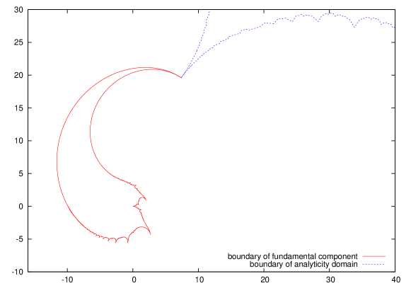
Figure 11. The domain of analyticity of ${\cal P}f_{0}(z)$ for $f_{0}(z)=z+z^{2}$, with the immediate parabolic basin indicated.

See Figure 11. Theorem 3.9 follows from Theorem 2.31 and a well-known folklore result:

Theorem 3.10.

The Julia set of the quadratic polynomial $f_{0}(z)=z+z^{2}$ is a Jordan curve. Orbits starting inside this curve converge to $0$; those starting outside converge to $\infty$. The dynamics of $f_{0}$ restricted to the Julia set is topologically conjugate to the angle-doubling map of the circle; specifically, there exists a unique continuous map $\rho:J(f_{0})\to{\mathbb{T}}$ such that

$$\rho(f_{0}(z))=2\rho(z)\operatorname{mod}1.$$

In the next subsection, we will provide a proof of Theorem 3.10; while it is fairly standard, the strategy used will be useful to us later in a more complicated situation.

3.3. The Julia set of $f_{0}(z)=z+z^{2}$ is a Jordan curve.

We begin by defining several useful local inverse branches of $f_{0}$, by choosing the appropriate branches of the square root in the formal expression

(3.2) $$f_{0}^{-1}(w)=\sqrt{w+1/4}-1/2.$$

We first cut the plane along the positive real ray $R\equiv[-1/4,+\infty)$ and denote

$${g_{0}}:{{\mathbb{C}}\setminus R}\to{\mathbb{H}}$$

the inverse branch with non-negative imaginary part. Similarly, we define

$${g_{1}}:{{\mathbb{C}}\setminus R}\to-{\mathbb{H}}$$

to be the inverse branch with negative imaginary part, so that ${g_{1}}\equiv 1-{g_{0}}$.

Finally, we define an inverse branch ${g}$ which fixes the parabolic point $z=0$. We slit the plane along the ray $(-\infty,-1/4]$, and select the branch of the square root in (3.2) with non-negative real part. In this way, we get

$${g}:{\mathbb{C}}\setminus(-\infty,-1/4]\to\{\operatorname{Re}z>-1/2\}.$$

We note that Taylor expansion of ${g}$ at $w=0$ begins with $w-w^{2}+\cdots$, and thus it also has a parabolic fixed point at the origin.

When needed, we will continuosly extend the three inverse branches defined above to the edges of the slits.

Proposition 3.11.

The branch ${g}$ maps ${\mathbb{C}}\setminus(-\infty,0]$ into itself.

Proof.

As already noted, the image of ${g}$ is contained in the half-plane $\{\operatorname{Re}z>-1/2\}$. Furthermore, since ${g}$ is a branch of the inverse of $f_{0}$, if ${g}(w)\in[-1/2,0)$, then $w\in f_{0}([-1/2,0))=([-1/4,0)\subset(-\infty,0)$, so the image under ${g}$ of ${\mathbb{C}}\setminus(-\infty,0]$ does not intersect $[-1/2,0)$ and so is contained in ${\mathbb{C}}\setminus(-\infty,0]$ ∎

Applying the Denjoy-Wolff Theorem, we obtain

Corollary 3.12.

The successive iterates ${{g}}^{n}$ converge to the constant $0$ – the parabolic point – uniformly on compact subsets of ${\mathbb{C}}\setminus(-\infty,0]$.

Next, we observe:

Proposition 3.13.

The intersection

$$J(f_{0})\cap{\mathbb{R}}=\{-1,0\}.$$

Proof.

Indeed, if $x>0$ then

$$f(x)=x+x^{2}>x\text{, and, furthermore, }f^{n}(x)>x+nx^{2}\to\infty,$$

and hence $(0,\infty)\subset F(f_{0})$. Since

$$f_{0}((-\infty,-1))=(0,\infty),$$

the same holds for $(-\infty,-1)$. Finally, $f_{0}$ maps the interval $(-1,0)$ to itself and $f_{0}(x)>x$ for $x$ in this interval, so $f_{0}^{n}(x)\to 0$. Hence, $(-1,0)\subset F(f)$ as well, as claimed. ∎

Define

$${\mathbf{A}}:=\{z:1/2<|z+1/2|<2\}.\,$$

i.e., ${\mathbf{A}}$ is an annulus, centered at the critical point $-1/2$, with inner radius $1/2$ and outer radius $2$. We collect some elementary facts about this annulus into the following proposition:

Proposition 3.14.

1. If $|z+1/2|\geq 2$ – i.e., if $z$ is outside the annulus – then $|f_{0}(z)+1/2|>|z+1/2|$, so $f_{0}(z)$ is again outside the annulus, and $|f^{n}_{0}(z)+1/2|$ goes monotonically to $\infty$.

2. If $|z+1/2|<1/2$ – i.e., if $z$ is strictly inside the annulus – then $|f_{0}(z)+1/4|<1/4$.

3. If $|z+1/2|<1/2$, then $f_{0}^{n}(z)\to 0$.

4. if $f(z)\in{\mathbf{A}}$, then $z\in{\mathbf{A}}$, i.e., $f_{0}^{-1}{\mathbf{A}}\subset{\mathbf{A}}$.

5. $J(f_{0})$ is contained in the closure $\overline{{\mathbf{A}}}$ of ${\mathbf{A}}$.

Proof.

Items (1) and (2) follow from elementary estimates. For (3): Since the open disk of radius $1/4$ about $-1/4$ is contained in the open disk of radius $1/2$ about $-1/2$, this latter disk is mapped into itself by $f_{0}$ and hence by all its iterates $f_{0}^{n}$. In particular, this sequence of iterates is uniformly bounded on the disk in question and so – by Montel’s Theorem – is a normal family. Furthermore, elementary considerations show that, for $-1<x<0$, $f_{0}^{n}(x)\to 0$. It follows then from Vitali’s Theorem that $f_{0}^{n}$ converges to the constant $0$ uniformly on compact sets of the open disk $\{|z+1/2|<1/2\}$.

From (1) and (2): If $z\notin{\mathbf{A}}$, then $f_{0}(z)\notin{\mathbf{A}}$, which is tautologically equivalent to (4). Finally, from (1), if $z$ is outside $\overline{{\mathbf{A}}}$, then $f_{0}^{n}(z)\to\infty$, so $z\notin J(f_{0})$, and, from (3). If $z$ is inside $\overline{{\mathbf{A}}}$, $f_{0}^{n}(z)\to 0$ so – again – $z\notin J(f_{0})$. ∎

To prove Theorem 3.10, we are going to show that $f_{0}^{-n}{\mathbf{A}}$ are a decreasing sequence of topological annuli which shrink down to a Jordan curve $J$. Points inside $J$ are attracted to the parabolic point; those outside are attracted to $\infty$. Thus, the Jordan curve $J$ contains the Julia set. Our argument also shows that the preimages (of arbitrary order) of the parabolic point $0$ under $f_{0}$ are dense in $J$, so the Julia set is the whole of $J$.

We define first

$${\mathbf{A}}_{0}:=\{z\in{\mathbf{A}}\,:\,\operatorname{Im}z>0\}\quad\text{and}\quad{\mathbf{A}}_{1}:=\{z\in{\mathbf{A}}\,:\,\operatorname{Im}z<0\},$$

and then, for any $n=2,\ldots$ and any sequence $i_{0}i_{1}\ldots i_{n-1}$ of $n$ 0’s and 1’s,

$${\mathbf{A}}_{i_{0}i_{1}\ldots i_{n-1}}:=\{z\in{\mathbf{A}}_{i_{0}}:f_{0}^{j}(z)\in{\mathbf{A}}_{i_{j}}\quad\text{for}\quad 1\leq j<n\}$$

We will refer to the sets ${\mathbf{A}}_{i_{0}\ldots i_{n-1}}$ as puzzle pieces (of level $n$.) It is easy to see that

• ${\mathbf{A}}_{i_{0}i_{1}\ldots i_{n-1}}$ is decreasing in $n$: ${\mathbf{A}}_{i_{0}\ldots i_{n-1}}\supset{\mathbf{A}}_{i_{0}\ldots i_{n}};$

• $f{\mathbf{A}}_{i_{0}i_{1}\ldots i_{n}}={\mathbf{A}}_{i_{1}\ldots i_{n}};$

• ${\mathbf{A}}_{i_{0}i_{1}\ldots i_{n}}={g_{i_{0}}}{\mathbf{A}}_{i_{1}\ldots i_{n}},$ and hence
  ${\mathbf{A}}_{i_{0}i_{1}\ldots i_{n-1}}={g_{i_{0}}}\circ{g_{i_{1}}}\circ\cdots\circ{g_{i_{j-1}}}{\mathbf{A}}_{i_{j}i_{j+1}\ldots i_{n-1}}\quad\text{for $1\leq j<n-1$.}$

Figure 4. There are $2^{n}$ puzzle pieces of level $n$. In the picture for level $n$, we also show the outlines of the puzzle pieces of level $n-1$, each of which contains two pieces of level $n$. The pieces of level $n$ can be labeled (successively, counterclockwise, starting from the positive real axis) with $0,1,\ldots,2^{n}-1$; the labeling used in the text is the binary representation of this one.

The main step in the argument is to show that the diameters of the puzzle pieces ${\mathbf{A}}_{i_{0}i_{1}\ldots i_{n-1}}$ go to zero as $n\to\infty$, uniformly in $i_{0}i_{1}\ldots i_{n-1}$. The strategy that we use is standard; it also appears in, e.g., [Lyu], Proposition 1.10.

Concretely, we define

$$\rho_{n}:=\sup\left\{\text{diam}({\mathbf{A}}_{i_{0}\ldots i_{n-1}}):i_{0}\ldots i_{n-1}\in\{0,1\}^{n}\right\}$$

Since ${\mathbf{A}}_{i_{0}\ldots i_{n-1}}\supset{\mathbf{A}}_{i_{0}\ldots i_{n}}$, the sequence $\rho_{n}$ is non-increasing in $n$, so

(3.3) $$\rho_{*}:=\lim_{n\to\infty}\rho_{n}$$

exists.

We will prove:

Proposition 3.15.

The limit $\rho_{*}=0.$

The first step is to argue that it suffices to consider binary sequences one at a time:

Lemma 3.16.

There is an infinite sequence $i_{0}i_{1}\ldots i_{n}\ldots$ so that

$$\operatorname{diam}(A_{i_{0}i_{1}\ldots i_{n}})\geq\rho_{*}\quad\text{for all $n$,}$$

i.e., a single descending chain of puzzle pieces with diameter converging to $\rho_{*}$.

Proof of Lemma 3.16.

A simple diagonal argument gives the existence of a sequence $i_{0}i_{1}\ldots i_{k}\ldots$ such that, for all $k$,

$$\lim_{n\to\infty}\sup\left\{\text{diam}({\mathbf{A}}_{i_{0},\ldots i_{k-1}i^{\prime}_{k}\ldots i^{\prime}_{k+n-1}}):i^{\prime}_{k}\ldots i^{\prime}_{k+n-1}\in\{0,1\}^{n}\right\}\geq\rho_{*}$$

Since $\text{diam}({\mathbf{A}}_{i_{0}i_{1}\ldots i_{n-1}})$ is non-increasing in $n$, it follows that

$$\text{diam}({\mathbf{A}}_{i_{0}i_{1}\ldots i_{k}})\geq\rho_{*}\quad\text{for all $k$,}$$

proving the lemma. ∎

Proof of Proposition 3.15.

We assume the contrary, that $\rho_{*}>0$ and we fix a sequence $i_{0}i_{1}\ldots$ as in the Lemma 3.16, i.e., so that $\text{diam}({\mathbf{A}}_{i_{0}i_{1}\ldots i_{k-1}})$ does not go to zero as $k\to\infty$. We consider separately the three cases:

1. $i_{j}$ is eventually 0;

2. $i_{j}$ is eventually 1;

3. $i_{j}$ takes both values $0$ and $1$ infinitely often.

We start with case (3). There are then infinitely many $j$’s so that

$$i_{j}=0\quad\text{and}\quad i_{j+1}=1$$

Let $j_{k}$ be a strictly increasing sequence of such $j$’s. Then, for each $k$,

$$f_{-j_{k}}:={g_{i_{0}}}\circ{g_{i_{1}}}\circ\cdots\circ{g_{i_{j_{k}-1}}}$$

is an analytic branch of the inverse of $f_{0}^{j_{k}}$ mapping ${\mathbf{A}}_{01}$ bijectively to ${\mathbf{A}}_{i_{0}\ldots i_{j_{k}+1}}$. The closure of ${\mathbf{A}}_{01}$ does not intersect the closure of the postcritical set of $f_{0}$; we let $U$ be an bounded simply connected open neighborhood of $\overline{{\mathbf{A}}_{01}}$ disjoint from the postcritical set. Then each $f_{-j_{k}}$ has an extension to a branch of the inverse of $f_{0}^{j_{k}}$ defined and analytic on $U$; we denote this extension also by $f_{-j_{k}}$.

We next want to argue that the $f_{-j_{k}}$ are uniformly bounded on $U$ and hence form a normal family there. We can see this as follows: Let $\hat{U}$ be a neighborhood of $\infty$ which is forward-invariant under $f_{0}$ and disjoint from $U$. Then, if $f_{j_{k}}(z)$ were in $\hat{U}$ (for some $k$ and some $z\in U$), we would have – since $f_{j_{k}}$ is an inverse branch of $f_{0}^{j_{k}}$ and $\hat{U}$ is forward invariant –

$$z=f_{0}^{j_{k}}(f_{-j_{k}}(z))\in\hat{U},$$

which is impossible since by hypothesis $z\in U$ and $U$ is disjoint from $\hat{U}$. Thus, the sets $f_{-j_{k}}U$ are all disjoint from $\hat{U}$, so $(f_{-j_{k}})$ is uniformly bounded on $U$, as desired.

By Montel’s Theorem, there is a subsequence of $(j_{k})$ along which $f_{-j_{k}}$ converges uniformly on compact subsets of $U$. By adjusting the notation, we can assume that the sequence $(f_{-j_{k}})$ itself converges; we denote its limit by $h$. Since

$$\text{diam}(f_{-j_{k}}{\mathbf{A}}_{01})=\text{diam}({\mathbf{A}}_{i_{0}\ldots i_{j_{k}+1}})$$

does not go to zero as $k\to\infty$, and since $f_{-j_{k}}$ converges uniformly on the closure of ${\mathbf{A}}_{01}$, the limit $h$ is non-constant.

Let $z_{0}:={g_{0}}({g_{1}}(-1))\in{\mathbf{A}}_{01}\cap J(f_{0})$. Since the Julia set if backward-invariant under $f_{0}$ and closed,

$$w_{0}:=h(z_{0})=\lim_{k\to\infty}f_{-j_{k}}(z_{0})$$

is again in the Julia set. Since $h$ is non-constant, $h{\mathbf{A}}_{01}$ is an open neighborhood of $w_{0}$; let $W$ be another open neighborhood whose closure is compact and contained in $h{\mathbf{A}}_{01}$. A straightforward application of Rouché’s theorem shows that

$$f_{-j_{k}}{\mathbf{A}}_{01}\supset W\quad\text{for sufficiently large $k$.}$$

Since $f_{-j_{k}}$ is a branch of the inverse of $f_{0}^{j_{k}}$, it follows that

(3.4) $$f_{0}^{j_{k}}W\subset{\mathbf{A}}_{01}\quad\text{for all sufficiently large $k$.}$$

We are going to deduce from (3.4) that

$$|f_{0}^{n}(w)+1/2|\leq 2\quad\text{for $w\in W$ and $n\geq 0$,}$$

which by Montel’s theorem contradicts the fact that $w_{0}\in W$ is in the Julia set. Suppose, therefore, that $|f_{0}^{n}(w)+1/2|>2$ for some $w\in W$ and some $n$. Then, by Proposition 3.14(1),

$$|f_{0}^{j_{k}}(w)+1/2|>2\quad\text{for all $k$ with $j_{k}\geq n$.}$$

Since

$$|z+1/2|\leq 2\quad\text{for all $z\in{\mathbf{A}}$,}$$

this contradicts (3.4), and so completes the proof in case 3.

We turn next to case (1) above, and deal first with the situation $i_{j}=0$ for all $j$. We write temporarily

$${\mathbf{A}}^{(n)}:={\mathbf{A}}_{\underbrace{0\cdots 0}_{\text{$n$ terms}}}=({g_{0}})^{n-2}{\mathbf{A}}_{00}$$

Now ${g_{0}}$ maps ${\mathbf{A}}_{00}$ into itself, and ${g_{0}}={g}$ on ${\mathbf{A}}_{00}$, so we can write

$${\mathbf{A}}^{(n)}={{g}}^{n-2}{\mathbf{A}}_{00}.$$

By Corollary 3.12 and local properties of parabolic dynamics near $0$,

$${{g}}^{n-2}\to 0\quad\text{uniformly on ${\mathbf{A}}_{00}$},$$

so

$$\text{diam}({\mathbf{A}}^{(n)})\to 0\quad\text{as $n\to\infty$.}$$

Next consider sequences of the form $i_{0}i_{1}\cdots i_{k}00\cdots$, and use the formula

$${\mathbf{A}}_{i_{0}\ldots i_{k}\underbrace{0\cdots 0}_{\text{$n$ terms}}}={g_{i_{0}}}\circ{g_{i_{1}}}\circ\cdots\circ{g_{i_{k}}}A^{(n)}.$$

The mapping ${g_{i_{0}}}\circ{g_{i_{1}}}\circ\cdots\circ{g_{i_{k}}}$ extends to be continuous on $\overline{{\mathbf{A}}_{00}}$, and $\text{diam}(A^{(n)})\to 0$ by what we just proved, so

$$\text{diam}({\mathbf{A}}_{i_{0}\ldots i_{k}\underbrace{0\cdots 0}_{\text{$n$ terms}}})\to 0\quad\text{as $n\to\infty$.}$$

A similar argument, using ${g_{1}}={g}$ on ${\mathbf{A}}_{11}$ shows that

$$\text{diam}({\mathbf{A}}_{i_{0}\ldots i_{k}\underbrace{1\cdots 1}_{\text{$n$ terms}}})\to 0\quad\text{as $n\to\infty$.}$$

∎

Let ${\mathbf{i}}=(i_{j})_{j=0}^{N}$ be a finite or infinite sequence ($N\leq\infty$) of $0$’s and $1$’s. We interpret it as a binary representation of an element of the circle ${\mathbb{R}}/{\mathbb{Z}}$:

$${\underline{\mathbf{i}}}_{2}\equiv\sum_{j=0}^{N}i_{j}2^{j+1}\bmod{{\mathbb{Z}}}.$$

For any such dyadic sequence,

$$\overline{{\mathbf{A}}_{i_{0}}}\supset\overline{{\mathbf{A}}_{i_{0}i_{1}}}\supset\cdots\supset\overline{{\mathbf{A}}_{i_{0}\ldots i_{n}}}\supset\ldots$$

is a nested sequence of compact sets in ${\mathbb{C}}$ with diameter going to 0, so its intersection contains exactly one point, which we denote by $\hat{z}({\mathbf{i}})$. Since any ${\mathbf{A}}_{i_{0}\ldots i_{n-1}}$ contains $g_{i_{0}}g_{i_{1}}\cdots g_{i_{n-1}}(-1)\in J(f_{0})$, each $\hat{z}({\mathbf{i}})\in J(f_{0})$. It is immediate from the construction that ${\mathbf{i}}\mapsto\hat{z}({\mathbf{i}})$ is continuous from $\{0,1\}^{\mathbb{N}}$ to ${\mathbb{C}}$. It is not injective, but its non-injectivity is of a simple and familier nature:

Lemma 3.17.

Let ${\mathbf{i}}=i_{0}i_{1}\ldots i_{n-1}$ and ${\mathbf{i}}^{\prime}=i^{\prime}_{0}i^{\prime}_{1}\ldots i^{\prime}_{n-1}$ be two finite dyadic sequences of equal length such that

$$\overline{{\mathbf{A}}_{{\mathbf{i}}}}\cap\overline{{\mathbf{A}}_{{\mathbf{i}}^{\prime}}}\neq\emptyset.$$

Then either ${\underline{\mathbf{i}}}_{2}={\underline{\mathbf{i}^{\prime}}}_{2}$ or ${\underline{\mathbf{i}}}_{2}={\underline{\mathbf{i}^{\prime}}}_{2}\pm 2^{-n}.$

The proof is a straightforward induction in $n$ which we leave to the reader. As a corollary, we get:

Corollary 3.18.

Let ${\mathbf{i}}$ and ${\mathbf{i}^{\prime}}$ be two infinite dyadic sequences. Then

$$\hat{z}({\mathbf{i}})=\hat{z}({\mathbf{i}^{\prime}})\quad\text{if and only if}\quad{\underline{\mathbf{i}}}_{2}={\underline{\mathbf{i}^{\prime}}}_{2}$$

Proof.

For any ${\mathbf{i}}=i_{0}\cdots i_{n}\cdots$, and any $n$

$$|{\underline{\mathbf{i}}}_{2}-\underline{i_{0}\cdots i_{n-1}}_{2}|\leq 2^{-n}.$$

Hence, if ${\underline{\mathbf{i}}}_{2}\neq{\underline{\mathbf{i}^{\prime}}}_{2}$ and $n$ is large enough so that

$$|{\underline{\mathbf{i}}}_{2}-{\underline{\mathbf{i}^{\prime}}}_{2}|>3\times 2^{-n},$$

then

$$|\underline{i_{0}\cdots i_{n-1}}_{2}-\underline{i^{\prime}_{0}\cdots i^{\prime}_{n-1}}_{2}|>2^{-n},$$

which by Lemma 3.17 implies that $\overline{{\mathbf{A}}_{i_{0}\cdots i_{n-1}}}$ and $\overline{{\mathbf{A}}_{i^{\prime}_{0}\cdots i^{\prime}_{n-1}}}$ are disjoint, and hence that $\hat{z}({\mathbf{i}})\neq\hat{z}({\mathbf{i}^{\prime}})$.

Conversely, if ${\underline{\mathbf{i}}}_{2}={\underline{\mathbf{i}^{\prime}}}_{2}$, then either ${\mathbf{i}}={\mathbf{i}^{\prime}}$ or – possibly after interchanging the two sequences – ${\mathbf{i}}$ has the form $i_{0}i_{1}\ldots i_{m-1}0111\ldots$ and ${\mathbf{i}^{\prime}}$ the form $i_{0}i_{1}\ldots i_{m-1}1000\ldots$ and from this it follows easily that $\overline{{\mathbf{A}}_{i_{0}\cdots i_{n}}}$ and $\overline{{\mathbf{A}}_{i^{\prime}_{0}\cdots i^{\prime}_{n}}}$ intersect for all $n$ and hence that $\hat{z}({\mathbf{i}})=\hat{z}({\mathbf{i}^{\prime}})$ ∎

Hence, there is an injective mapping $\theta\mapsto z(\theta)$, from the circle ${\mathbb{R}}/{\mathbb{Z}}$ to ${\mathbb{C}}$, such that

$$\hat{z}({\mathbf{i}})=z({\underline{\mathbf{i}}}_{2})\quad\text{for all ${\mathbf{i}}$.}$$

Proposition 3.19.

The mapping $z(\,.\,)$ is a homeomorphism from the circle onto the image $J$ of ${\mathbf{i}}\mapsto\hat{z}({\mathbf{i}})$. In particular, $J$ is a Jordan curve.

Proof.

$z(\,.\,)$ is injective by construction, and its continuity follows easily from the fact that $\operatorname{diam}({\mathbf{A}}_{i_{0}\cdots i_{n-1}})\to 0$. It is therefore a homeomorphism by the standard topological fact that an injective continuous mapping from a compact space (to a Hausdorff space) is a homeomorphism. ∎

It remains to show that

Proposition 3.20.

$J=J(f_{0})=\bigcap_{n\geq 0}f_{0}^{-n}\overline{A}$.

Proof.

We show

1. $J\subset J(f_{0})$

2. $J(f_{0})\subset\bigcap_{n\geq 0}f_{0}^{-n}\overline{A}$

3. $\bigcap_{n\geq 0}f_{0}^{-n}\overline{A}\subset J$

(1) If $z\in J$, then $\{z\}=\bigcap\overline{{\mathbf{A}}_{i_{0}\cdots i_{n-1}}}$ for some sequence $i_{0}i_{1}\ldots$. Since $A_{i_{0}\cdots i_{n-1}}$ contains $g_{i_{0}}\circ\cdots\circ g_{i_{n-1}}(-1)\in J(f_{0})$, and since $\operatorname{diam}(A_{i_{0}\cdots i_{n-1}})\to 0$, $z\in\overline{J(f_{0})}=J(f_{0}).$.

(2) This proof has essentially already been given: If $z\notin\bigcap_{n\geq 0}f_{0}^{-n}\overline{A}$, then some $f_{0}^{n}(z)\notin\overline{A}$, so – by the elementary properties of the basic annulus ${\mathbf{A}}$ (Proposition 3.14) – $f_{0}^{n}(z)$ converges either to $0$ or to $\infty$, so $z\notin J(f_{0})$.

(3) Assume $z\in\bigcap_{n\geq 0}f_{0}^{-n}\overline{A}$, i.e., $f_{0}^{n}(z)\in\overline{A}$ for all $n$. We consider two cases:

• $f_{0}^{n}(z)\notin{\mathbb{R}}$ for all $n$. Put $i_{n}=0$ of $1$ according as $f_{0}^{n}(z)$ is in the upper or lower half-plane. Then $z\in{\mathbf{A}}_{i_{0}\cdots i_{n-1}}$ for all $n$, so $z=\hat{z}({\mathbf{i}})\in J$.

• $f_{0}^{n}(z)\in{\mathbb{R}}$ for some $n$. The intersection of $\overline{{\mathbf{A}}}$ with ${\mathbb{R}}$ is the union of the two intervals $[-2.5,-1]$ and $[0,1.5]$, and the first of these maps into the positive real axis, which is mapped into itself. Hence $f_{0}^{n}(z)$ is eventually in $[0,1.5]$. But the only orbit staying forever in $[0,1.5]$ is the fixed point $0$, so $z$ must be a preimage of finite order of $0$. It is then straighforward to show that there is a sequence of the form $i_{0}i_{1}\cdots i_{n-1}000\cdots$ with $z=\hat{z}({\mathbf{i}})$

∎

This completes the proof of Theorem 3.10 We note further that

$$f_{0}(\hat{z}(i_{0}i_{1}i_{2}\cdots))=\hat{z}(i_{1}i_{2}\cdots)\quad\text{for all binary sequences $i_{0}i_{1}\cdots$.}$$

from which it follows that:

Proposition 3.21.

The map $\theta\mapsto z(\theta)$ conjugates $\theta\mapsto 2\cdot\theta$ on ${\mathbb{R}}/{\mathbb{Z}}$ to $f_{0}$ on its Julia set $J(f_{0})$.

3.4. Covering properties of Écalle-Voronin invariant of $f_{0}$

For a parabolic germ $f(z)$ of the form (2.2) we will denote ${\mathbf{h}}_{f}$ its Écalle-Voronin invariant. We remind the reader, that the pair of germs ${\mathbf{h}}_{f}=(h^{+},h^{-})$ is defined up to pre- and post-composition with a multiplication by a non-zero constant.

We approach the discussion of covering properties of ${\mathbf{h}}_{f_{0}}$ indirectly, by introducing a different, more convenient, dynamical model.

By Riemann Mapping Theorem, there is a conformal isomorphism $\psi$ from $B_{0}$ to the cut plane ${\mathbb{C}}\setminus(-\infty,0]$ sending $-1/2$ (the critical point of $f_{0}$) to $-1$. These conditions do not fix $\psi$ uniquely, but it is not difficult to see that $\psi$ can be chosen so that $\psi^{\prime}(-1/2)>0$ and, under this condition, becomes unique. Because of uniqueness, and because $B_{0}$ and the cut plane are invariant under complex conjugation, $\psi$ commutes with complex conjugation. It must therefore map $(-1,0)$ to $(-\infty,0)$, these being respectively the real points of $B_{0}$ and those of the cut plane. Since $\psi^{\prime}(-1/2)>0$, $\psi$ is strictly increasing on $(-1,0)$, and $\lim_{x\to 0^{-}}\psi(x)=0$.

Define an analytic mapping $K$ of the cut plane to itself by

(3.5) $$K=\psi\circ f_{0}\circ\psi^{-1}.$$

So defined, $K$ is a real-symmetric analytic degree-2 branched cover:

$$K:{\mathbb{C}}\setminus[0,\infty)\to{\mathbb{C}}\setminus[0,\infty).$$

By construction, $-1$ is a critical point of $h$, and the corresponding critical value is $\psi(-1/4)$. There is a simple explicit formula for $h$:

Proposition 3.22.

The mapping $K(z)$ is the Koebe function

(3.6) $$K(z)=\frac{z}{(z-1)^{2}}$$

Proof.

For $x\in[0,\infty)$ and small positive $\epsilon$, $K(x+i\epsilon)$ and $K(x-i\epsilon)$ are complex conjugates. As $\epsilon\to 0^{+}$, $x+i\epsilon$ converges to the boundary of the cut plane, so $\psi^{-1}(x+i\epsilon)$ converges to the boundary of $B_{0}$, so $f_{0}(\psi^{-1}(x+i\epsilon))$ also converges to the boundary of $B_{0}$, so $K(x+i\epsilon)$ converges to the boundary $[0,\infty]$ of the cut plane.

We apply Schwarz reflection to see that $K$ can be extended analytically through $[0,\infty)$. The above argument does not rule out that $K(x+i\epsilon)$ goes to $\infty$. To get around this, we recall that $K$ is a degree-2 branched cover, and that, on a small disk about the critical point $-1$, it takes on every value near the critical value $K(-1)$ twice. Hence, $K(x+i\epsilon)$ stays away from $K(-1)$, so Schwarz reflection can be applied without difficulty to the function $1/(K(-1)-K(z))$, which is bounded on a neighborhood of the positive axis.

Thus, $K$ extends to a function meromorphic on the finite plane. Since $1/(K(-1)-K(z))$ is bounded near $\infty$, $K$ is also meromorphic at $\infty$, and hence, it is a rational function. Since it takes each finite non-real value exactly twice, it has degree 2. It never takes on a value in $[0,\infty]$ anywhere off $[0,\infty]$ so it must map $[0,\infty]$ to itself, with each point having two preimages, counted with multiplicity. As $x$ runs up the positive axis, $K(x)$ starts at $0$ and runs up, reaching $\infty$ at some finite $a$; it then runs back down, approaching $0$ as $x\to\infty$. The pole at $a$ must have order 2, so $K(z)$ must have the form

$$K(z)=(bz^{2}+cz+d)/(z-a)^{2}.$$

From $K(0)=K(\infty)=0$, we have $b=d=0$. Thus,

$$K(z)=cz/(z-a)^{2}$$

for some constant $c$, which clearly must be positive. By a simple calculation, a function of this form has only one (finite) critical point, at $-a$, so $a=1$. It remains only to show $c=1$.

We saw above, from elementary considerations, that $\psi(x)\to 0$ as $x\to 0^{-}$. Hence, for small negative $x$,

$$K^{n}(\psi(x))=\psi(f_{0}^{n}(x))\to 0,$$

so there are at least some $K$-orbits converging to $0$; this rules out $c>1$, so we need only show that $c<1$ is also impossible.

By Theorem 3.10, and Carathéodory Theorem, $\psi$ has a continuous extension to the boundary $J(f_{0})$ of $B_{0}$ – which we continue to denote by $\psi$. The extension is not a homeomorphism; it identifies complex conjugate pairs on $J(f_{0})$. A useful invertibility property can be formulated as follows: $J(f_{0})\setminus{-1,0}$ is a disjoint union of two Jordan arcs, and the extended $\psi$ maps each of these arcs homeomorphically to $(0,\infty)$. Note that the conjugation equation, written in the form

$$K\circ\psi=\psi\circ f,$$

extends by continuity to $\overline{B_{0}}$. Because $f_{0}$ on $J(f_{0})$ is conjugate to $s\mapsto 2s$ on ${\mathbb{T}}$, there exist infinite backward orbits for $f_{0}$ in $J(f_{0})$ which converge to $0$, i.e., sequences $z_{0}$, $z_{-1}$, $z_{-2}$, …with $z_{-n+1}=f(z_{-n})$ and $z_{-n}\to 0$. Then $\psi(z_{-n})\to 0$ and $K(\psi(z_{-n})=\psi(z_{-n+1})$, that is, $(\psi(z_{-n})$ is a backward orbit for $K$ converging to $0$. This rules out $c<1$, so the only remaining possibility is $c=1$, so the formula (3.6) is proved.

∎

We note several other contexts in which the Koebe function (3.6) comes up. It is, of course, the essentially unique function univalent on the unit disk which saturates the Koebe distortion estimates. (See, for example, [Co], Theorem 7.9 and p. 31.)

Furthermore, and perhaps more instructively for our study, one can deduce from the above discussion that $K(z)$ is the conformal mating (see [Do1]) of the map $f_{0}$ with the Chebysheff quadratic polynomial $f_{-2}(z)=z^{2}-2.$

We next develop an important piece of technique:

Proposition 3.23.

Let $f_{1}$, $f_{2}$ each have a normalized simple parabolic point at $0$, and assume that their restrictions to their respective principal basins are conformally conjugate, i.e., that there is a conformal isomorphism $\varphi:B^{f_{1}}_{0}\to B^{f_{2}}_{0}$ so that

(3.7) $$f_{1}=\varphi^{-1}\circ f_{2}\circ\varphi\quad\text{on $B^{f_{1}}_{0}$.}$$

Assume further that $\varphi$ and $\varphi^{-1}$ extend continuously to the boundary point $0$ of $B^{f_{1}}_{0}$ respectively $B^{f_{2}}_{0}$. Then there is a conformal isomorphism $\psi:W^{+}_{f_{1}}\to W^{+}_{f_{2}}$, sending $0$ to $0$, and a non-zero constant $v$ so that

$$h^{+}_{f_{1}}=v\cdot h^{+}_{f_{2}}\circ\psi.$$

We begin with a few simple remarks. From the continuity of $\varphi$ at $0$, it follows that $\varphi(0)=0$:

$$\varphi(0)=\lim_{n\to\infty}\varphi(f_{1}^{n}(z))=f_{2}^{n}(\varphi(z))=0\quad\text{for any $z\in B^{f_{1}}_{0}$,}$$

It is easy to verify, again making use of continuity of $\varphi$ at $0$, that $\varphi$ maps attracting petals for $f_{1}$ to attracting petals for $f_{2}$, and that $\varphi^{-1}$ maps attracting petals for $f_{2}$ to attracting petals for $f_{1}$. For the proposition to make sense, we have to have chosen normalizations for attracting and repelling Fatou coordinates for the two mappings, but the choices are obviously immaterial. We fix – however we like – the normalization of $\phi^{(2)}_{A}$. Then $\phi_{A}^{(2)}\circ\varphi$ is an attracting Fatou coordinate for $f_{1}$, so, by the uniqueness of Fatou coordinates (Proposition 2.12), $\phi_{A}^{(2)}\circ\varphi-\phi_{A}^{(1)}$ is constant. For notational simplicity, we may assume

$$\phi_{A}^{(1)}=\phi_{A}^{(2)}\circ\varphi;$$

this has the effect of making the constant $v$ in the proposition equal to one.

The situation with repelling Fatou coordinates is more complicated. It is not true that $\varphi$ maps repelling petals to repelling petals, since $\varphi$ is only available on $B^{f_{1}}_{0}$ and repelling petals are not contained in $B_{0}$. What we have to work with instead is the weaker observation that $\varphi$ maps $f_{1}$-orbits coming out from $0$ in $B^{f_{1}}_{0}$ to the same kind of orbits for $f_{2}$. To exploit this observation, we need to develop some technique for a single function with a simple parabolic fixed point.

Let $f$ have the form (2.16); let $P_{R}$ be a repelling petal for $f$; and write $f^{-1}$ for the inverse of the restriction of $f$ to $P_{R}$. We define

$$\widetilde{P_{R}}:=\{z\in P_{R}:f^{-n}(z)\in B^{f}_{0}\text{ for $n=0,1,\ldots$}\}$$

In the usual way, it is straightforward to show that the image under $\operatorname{ixp}\circ\phi_{R}$ of $\widetilde{P_{R}}$ is independent of the petal $P_{R}$. We denote this image by $\widetilde{W}$; since $\widetilde{P_{R}}\subset P_{R}\cap B^{f}$, $\widetilde{W}$ is contained in ${\cal D}({\mathbf{h}}_{f})$.

Lemma 3.24.

1. Let $t\mapsto\tau(t),0\leq t\leq 1$ be a continuous arc in $P_{R}\cap B^{f}$ with $\tau(0)\in\widetilde{P_{R}}$. Then $\tau(1)\in\widetilde{P_{R}}$.

2. $\widetilde{P_{R}}$ is open (so its image $\widetilde{W}$ under $\operatorname{ixp}\circ\phi_{R}$ is also open.)

3. A connected component of $\widetilde{W}$ is also a connected component of ${\cal D}({\mathbf{h}})$. In other words, a component of ${\cal D}({\mathbf{h}})$ is either disjoint from $\widetilde{W}$ or contained in it.

4. If there is a continuous path $\tau$ in $P_{R}\cap B^{f}_{0}$ from $z$ to $f^{-1}(z)$, then $z\in\widetilde{P_{R}}$.

5. The components $W^{+}\setminus\{0\}$ and $W^{-}\setminus\{\infty\}$ of ${\cal D}({\mathbf{h}})$ are contained in $\widetilde{W}$.

Proof.

1. If $\tau(1)\notin\widetilde{P_{R}}$, there must be an $n$ so that $f^{-n}(\tau(1))\notin B_{0}^{f}$. Fix such an $n$, and let

$$t_{0}:=\inf\{t:f^{-n}(\tau(t))\notin B_{0}^{f}\}.$$

Since $\tau(\,.\,)$ and $f^{-1}$ are continuous and $B^{f}_{0}$ is open,

$$f^{-n}(\tau(t_{0}))\in\partial B^{f}_{0}\subset\partial B^{f},$$

so in particular $f^{-n}(\tau(t_{0}))\notin B^{f}$. But $B^{f}$ is backward-invariant under $f$ and the path $\tau$ is by assumption in $B^{f}$, so this is a contradiction.

2. If $z_{0}\in\widetilde{P_{R}}$ and $z$ is near enough to $z_{0}$, then the straight-line segment $[z_{0},z]$ is in $P_{R}\cap B^{f}$ and so – by 1. – in $\widetilde{P_{R}}$.

3. Since $\widetilde{W}$ is contained in ${\cal D}({\mathbf{h}})$, each component of $\widetilde{W}$ is contained in a component of ${\cal D}({\mathbf{h}})$. Let $U$ be a component of $\widetilde{W}$ and $V$ the component of ${\cal D}({\mathbf{h}})$ which contains it. If $U$ is not all of $V$, the relative boundary must be non-empty, i.e., there must exist a $w_{0}\in(\partial U)\cap V$. This $w_{0}$ is in ${\cal D}({\mathbf{h}})$, so it can be written as $w_{0}=\operatorname{ixp}\circ\phi_{R}(z_{0})$ with $z_{0}\in P_{R}\cap B^{f}$. Let $D$ be an open disk about $z_{0}$, small enough to be contained in $P_{R}\cap B^{f}$ and also so that $\operatorname{ixp}\circ\phi_{R}$ maps it homeomorphically into $V$. Since $\operatorname{ixp}\circ\phi_{R}(D)$ contains points of $\widetilde{W}$, $D$ contains points of $\widetilde{P_{R}}$, and it then follows from 1. that $D\subset\widetilde{P_{R}}$, so $z_{0}\in\widetilde{P_{R}}$, so $w_{0}\in\widetilde{W}$, contradiction.

4. We argue by induction on $n$ that $f^{-n}\tau\subset B^{f}_{0}$ for all $n$. This is true by hypothesis for $n=0$. Suppose it is true for $n$ but not for $n+1$. Then $f^{-(n+1)}(\tau(0))=f^{-n}(\tau(1))\in B^{f}_{0}$, but $f^{-(n+1)}(\tau(t_{0}))\in\partial B^{f}_{0}$ for some $t_{0}$. Then $f^{-(n+1)}(\tau(t_{0}))\notin B^{f}$, which contradicts $\tau(t_{0})\in B^{f}$ by backward invariance of $B^{f}$. The contradiction proves $f^{-n}\tau\subset B^{f}_{0}$ for all $n$, so, in particular, $f^{-n}(\tau(0))=f^{-n}(z)\in B^{f}_{0}$ for all $n$, i.e., $z\in\widetilde{P_{R}}$.

5. Since the resulting domain $\widetilde{W}$ does not depend on the repelling petal used to construct it, we may assume that $P_{R}$ is ample. Then a sector $\{z:0<|z|<\rho,\pi/2-\delta<\operatorname{Arg}(z)<\pi/2+\delta\}$, with $\rho$ and $\delta$ small enough, is contained in $P_{R}\cap B^{f}_{0}$. By 4. there is a sector of this form but with smaller $\delta$ and $\rho$ which is contained in $\widetilde{P_{R}}$, and, by the proof of Lemma 2.22, the image under $\operatorname{ixp}\circ\phi_{R}$ of this smaller sector is a punctured neighborhood of $0$. Thus, $\widetilde{W}$ intersects $W^{+}\setminus\{0\}$, so, by 3, $W^{+}\setminus\{0\}$ is one of the components of $\widetilde{W}$. The proof for $W^{-}\setminus\{\infty\}$ is similar.

∎

We return to the proof of Proposition 3.23; we are now now ready to construct the mapping $\psi$. We fix repelling petals $P^{(1)}_{R}$ for $f_{1}$ and $P_{R}^{(2)}$ for $f_{2}$. The situation is the familiar one: We need these petals to make a construction, but the objects constructed turn out not to depend on them. We let $\phi^{(1)}_{R}$ be a repelling Fatou coordinate for $f_{1}$ defined at least on $P^{(1)}_{R}$, and similarly $\phi^{(2)}_{R}$ for $f_{2}$. Let $w_{0}\in\widetilde{W_{1}}$, and write $w_{0}=\operatorname{ixp}\circ\phi_{R}^{(1)}(z_{0})$ with $z_{0}\in\widetilde{P^{(1)}_{R}}$. Then $z_{-n}:=f^{-n}(z_{0})$ is an outcoming orbit in $B^{f}_{0}$. Because $\varphi$ conjugates $f_{1}$ to $f_{2}$ (on their respective principal basins) and is continuous at $0$, $y_{-n}=\varphi(z_{-n})$ is an outcoming orbit for $f_{2}$. For sufficiently large $n$, $y_{-n}$ is in $P^{(2)}_{R}$. Take any $n_{0}$ so that $y_{-n}\in P^{(2)}_{R}$ for $n\geq n_{0}$, and set

$$\psi(w_{0})=\operatorname{ixp}\circ\phi^{(2)}_{R}(y_{-n_{0}})\in\widetilde{W_{2}}$$

It is easy to check that the result does not depend on the choices of repelling petals, preimage $z_{0}$, or number $n_{0}$ of steps back before applying $\operatorname{ixp}\circ\phi^{(2)}_{R}$, so we have constructed a mapping from $\widetilde{W_{1}}$ to $\widetilde{W_{2}}$. Each of the steps

$$w_{0}\mapsto z_{0}\mapsto z_{-n_{0}}=f^{-n_{0}}(z_{0})\mapsto y_{-n_{0}}\mapsto\psi(w_{0})=\operatorname{ixp}\circ\phi^{(2)}_{R}(y_{-n_{0}})$$

can be done in a neighborhood of each of the points involved by applying a local conformal isomorphism, so $\psi(\,.\,)$ is a local conformal isomorphism. Carrying out the same construction with $f_{1}$ and $f_{2}$ interchanged and $\varphi^{-1}$ in the role of $\varphi$ produces a mapping from $\widetilde{W_{2}}$ to $\widetilde{W_{1}}$ which inverts $\psi$, so $\psi$ is a global conformal isomorphism. Furthermore,

$$\begin{split}{\mathbf{h}}_{2}(\psi(w_{0}))&=\operatorname{ixp}\circ\phi^{(2)}_{A}(y_{-n_{0}})=\operatorname{ixp}\circ\phi^{(2)}_{A}(\varphi(y_{-n_{0}}))\\ &=\operatorname{ixp}\circ\phi^{(1)}_{A}(z_{-n_{0}})=\operatorname{ixp}\circ\phi^{(1)}_{A}(z_{0})={\mathbf{h}}_{1}(w_{0})\end{split}$$

The mapping $\psi$ just constructed is a more global version of the one in the proposition. To complete the proof of the proposition, we need to show

1. $\psi$ maps $W^{+}_{1}\setminus\{0\}$ to $W^{+}_{2}\setminus\{0\}$.

2. $\psi$ extends analytically to map $0$ to $0$

Proof of (1): Since $\psi:\widetilde{W_{1}}\to\widetilde{W_{2}}$ is a homeomorphism, it maps components to components. We know from 3 of Lemma 3.24 that $W^{+}_{1}\setminus\{0\}$ is a component of $\widetilde{W_{1}}$; we have only to show that the component it maps to is $W_{2}^{+}\setminus\{0\}$. To do this, choose ample petals $P^{(1)}_{A}$ and $P^{(1)}_{R}$ for $f_{1}$, and let $t\mapsto\lambda_{1}(t)$ be an arc in $P^{(1)}_{A}\cap P^{(1)}_{R}$, ending at $0$, which is mapped by $\phi^{(1)}_{A}$ to an upward vertical ray. By the asymptotic estimate for Fatou coordinates, $\lambda$ projects under $\operatorname{ixp}\circ\phi^{(1)}_{R}$ to an arc $\widetilde{\lambda_{1}}$ in $\widetilde{W_{1}}$ ending at $0$. Let $\lambda_{2}:=\varphi\circ\lambda_{1}$. It is then immediate that $\lambda_{2}$ maps under $\phi^{(2)}_{A}$ to an upward vertical ray.

Claim: $\lambda_{2}$ is tangent to the positive imaginary axis at $0$.

Accepting the claim for the moment: We can then project $\lambda_{2}$ under $\operatorname{ixp}\circ\phi^{(2)}_{R}$ to an arc $\widetilde{\lambda_{2}}$ in $\widetilde{W_{2}}$. By the asymptotic estimates on Fatou coordinates, $\widetilde{\lambda_{2}}$ ends at $0$. By the construction of $\psi$,

$$\widetilde{\lambda_{2}}=\psi\circ\widetilde{\lambda_{1}}.$$

Thus: $\psi(W^{+}_{1}\setminus\{0\})$ intersects $W^{+}_{2}$ and hence, by connectedness, $\psi(W^{+}_{1}\setminus 0)=W^{+}_{2}\setminus\{0\}$.

Proof of claim: It would be immediate if we knew that a terminal subarc of $\lambda_{2}$ is contained in an attracting petal. Rather than prove this directly, we argue as follows. Let $P^{(2)}_{A}$ be an attracting petal for $f_{2}$ which maps under $\phi^{(2)}_{A}$ to a right half-plane. Since $\lambda_{2}$ is contained in $B^{f}$, there is an $n$ so that $f_{1}^{n}(\lambda_{s}(0))\in P^{(2)}_{A}$. Since $\operatorname{Re}(\phi^{(2)}_{A})$ is constant on $\lambda_{2}$, $\lambda_{2}(t)$ stays in $P^{(2)}_{A}$, and, as already noted, approaches $0$ as $t\to 1^{-}$. By the crude estimates on Fatou coordinates, $f_{2}^{n}\circ\lambda_{2}$ is tangent to the positive imaginary axis at $0$. Applying an analytic local inverse of $f_{2}$ $n$ times proves the claim.

Proof of (2): This can be proved in a straightforward way using the crude local estimates on Fatou coordinates, but it is quicker to argue that

$$\psi=(h^{+}_{2})^{-1}\circ h^{+}_{1}\quad\text{on a punctured neighborhood of $0$},$$

(where $(h^{+}_{2})^{-1}$ means an analytic local inverse of $h^{+}_{2}$, which exists since $h^{+}_{2}$ has a simple zero at $0$) and to note that the right-hand side is analytic at $0$. To prove the preceding equation, we invoke the general formula $h^{+}_{1}=h^{+}_{2}\circ\psi$ and note that, by (1), $\psi$ and $(h_{2}^{+})^{-1}\circ h_{1}^{+}$ agree at points of the form $\widetilde{\lambda_{1}}(t)$ for $t$ near enough to 1. The assertion then follows by analytic continuation. The proof of Proposition 3.23 is thus completed. $\Box$

Definition 3.2.

For $K$ as in (3.6), let us select a real symmetric Fatou coordinate $\phi^{K}_{R}$, and a Fatou coordinate $\phi^{K}_{A}$ so that

$${\mathbf{h}}_{K}^{\prime}(0)=1\text{ and }{\cal D}(h^{+}_{K})={\mathbb{D}},\;{\cal D}(h^{-}_{K})={\mathbb{C}}\setminus{\mathbb{D}}\text{, where }{\mathbf{h}}_{K}=(h^{+}_{K},h^{-}_{K}).$$

We will denote thus normalized map ${\mathbf{h}}_{K}$ by ${\mathbf{k}}=(k^{+},k^{-})$ for the remainder of this paper.

In view of the above discussion, we note:

Proposition 3.25.

There exist $v\neq 0$ and $\theta\in{\mathbb{R}}$ such that

$${\mathbf{h}}_{f_{0}}=v\cdot{\mathbf{k}}\circ\psi(e^{2\pi i\theta}z),\text{ where }\psi:{\mathbb{D}}\to\hat{W}^{+}$$

is the conformal Riemann mapping, which satisfies $\psi(0)=0,$ $\psi^{\prime}(0)>0$.

We show:

Theorem 3.26.

${\mathbf{h}}_{f_{0}}$ has

• exactly one critical value $v:=\operatorname{ixp}\circ\phi_{A}(-1/4)$

• exactly two asymptotic values $0$ and $\infty$.

Proof.

To show that the above-defined $v$ is the only possible critical value of ${\mathbf{h}}_{f_{0}}$, we write

$${\mathbf{h}}_{f_{0}}=\bigl{(}\operatorname{ixp}\circ\phi_{A}\bigr{)}\circ\bigl{(}\operatorname{ixp}\circ\phi_{R}\bigr{)}^{-1},$$

for an appropriate branch of the inverse. Whatever inverse branch is used, its derivative does not vanish. Hence, a critical value of ${\mathbf{h}}_{f_{0}}$ is a critical value $\bigl{(}\operatorname{ixp}\circ\phi_{A}\bigr{)}$, i.e., the image under $\operatorname{ixp}(\,.\,)$ of a critical value of $\phi_{A}$. Since $-1/4$ is the unique critical value of $f_{0}$, it follows from Proposition 2.13 that the critical values of $\phi_{A}$ have the form $\phi_{A}(-1/4)-n$, $n\geq 1$. Since $\operatorname{ixp}(\,.\,)$ is 1-periodic, $v$ is the unique critical value of $\operatorname{ixp}\circ\phi_{A}$.

We turn to determining the asymptotic values of ${\mathbf{h}}_{f_{0}}$. We show that the asymptotic values of the restriction ${\mathbf{h}}_{f_{0}}|_{\hat{W}^{+}}$ are $\{0,\infty\}$; the argument for ${\mathbf{h}}_{f_{0}}|_{\hat{W}^{-}}$ is identical. To simplify geometric considerations, we invoke Proposition 3.25, and present the proof for ${\mathbf{k}}$.

We need a number of elementary facts about $K$ which we summarize below for ease of reference:

Proposition 3.27.

The Koebe function $K(z)=z/(1-z)^{2}$ is a degree-2 ramified cover $\hat{{\mathbb{C}}}\to\hat{{\mathbb{C}}}$; its critical values are $-1/4$ and $\infty$; the corresponding critical points are $-1$ and $+1$. The interval $[0,\infty]$ is fully invariant under $h$; the interval $(-\infty,0]$ is forward invariant.

The interval $[-\infty,-1/4]$ contains both of the critical values of $h$, so $h$ is a cover in the strict sense above ${\mathbb{C}}\setminus(-\infty,-1/4]$. In other words: $h$ admits two analytic right-inverses defined on the cut plane ${\mathbb{C}}\setminus(-\infty,-1/4]$. One of these inverse branches sends $0$ to $0$; the other sends $0$ to its other preimage $\infty$. At the cost of introducing a little ambiguity, we will write simply $K^{-1}$ for the inverse branch which is regular at $0$. A straightforward elementary calculation shows that the preimage of $(-\infty,0]$ under $h$ is the unit circle, so the image of $K^{-1}$ is the unit disk ${\mathbb{D}}$.

Proposition 3.28.

The inverse branch $K^{-1}$ maps the open upper (respectively lower) half-plane into itself. It also maps ${\mathbb{C}}\setminus(-\infty,0]$ into itself. The sequence of iterates $(K^{-1})^{n}$ converges uniformly to $0$ on compact subsets of ${\mathbb{C}}\setminus(-\infty,0]$. Any repelling Fatou coordinate extends to a univalent analytic function on ${\mathbb{C}}\setminus(-\infty,0]$.

Proof.

The proof may be given as an application of Denjoy-Wolff Theorem, however, a more direct argument is possible in our case.

Elementary considerations show that the upper half-plane is mapped into itself by $K^{-1}$, and similarly for the lower half-plane. Furthermore,

$$K^{-1}:{\mathbb{C}}\setminus(-\infty,0]\longrightarrow{\mathbb{C}}\setminus(-\infty,0].$$

By Montel’s theorem, the sequence of iterates $(K^{-1})^{n}$ is a normal family on ${\mathbb{C}}\setminus(-\infty,0]$. Elementary considerations show that $(K^{-1})^{n}(x)\to 0$ for $x$ real, positive, and small. By Vitali’s theorem, $(K^{-1})^{n}$ converges uniformly to $0$ on compact subsets of ${\mathbb{C}}\setminus(-\infty,0]$

The preceding assertion says that

$$B^{K^{-1}}_{0}={\mathbb{C}}\setminus(-\infty,0]$$

Note that any $K^{-1}$-orbit starting in $(-1/4,0)$ gets in finitely many steps into $(-1,-1/4]$, which is outside $\operatorname{Dom}(K^{-1})$. Thus, $(-1/4,0)$, although in $\operatorname{Dom}(K^{-1})$, is outside of $B^{K^{-1}}$. Using repeatedly the functional equation

$$\phi_{R}(K^{-1}(z))=\phi_{R}(z)-1,$$

we see that any repelling Fatou coordinate extends (uniquely) to a function defined on all of ${\mathbb{C}}\setminus(-\infty,0]$ and satisfying the above functional equation everywhere. The extended function is analytic; from the univalence of $K^{-1}$ and the fact that repelling Fatou coordinates are univalent on small petals, the extended function is also univalent. ∎

Next we introduce – in the context of the particular mapping $K$ – a useful dynamically-defined family of arcs which come up, with minor variations, at a number of places in this work. Let $\alpha$ be a real number so that

(3.8) $$\operatorname{Re}(\phi_{A}(-1))<\alpha<\operatorname{Re}(\phi_{A}(-1/4))\,(=\operatorname{Re}(\phi_{A}(-1))+1.)$$

Proposition 3.29.

There is an attracting petal $P$ which maps under $\phi_{A}$ to the right half-plane $\{u+iv:u>\alpha\}$.

For $\alpha$ a sufficiently large real number, this proposition is part of the local theory of parabolic fixed points. Showing that, in the present situation, any $\alpha>\operatorname{Re}(\phi_{A}(-1))$ is large enough depends on some covering properties of $K$. We omit the proof here.

The boundary of $P$ can be written as $\{0\}\cup\gamma$, where $\gamma$ is an arc in the cut plane ${\mathbb{C}}\setminus[0,\infty)$ which approaches the parabolic point $0$ at both ends. The arc $\gamma$ is a component of the preimage under $\phi_{A}$ of the vertical line $\{\alpha+iv:-\infty<v<\infty\}$; we give it the counterclockwise orientation, corresponding to the decreasing orientation for the vertical line: $\operatorname{Im}(\phi_{A}(z))$ runs from $+\infty$ to $-\infty$ as $z$ traverses $\gamma$ in the counterclockwise sense. This can be seen using the crude asymptotic formula $\phi_{A}(z)\approx-1/z$, valid for small $z$ not too near to the positive real axis.

We will speak of an arc $s\mapsto\sigma(s)$, defined and continuous for $0<s<1$ – i.e., without beginning or end point – as an open arc. We say that such an arc starts at $z_{0}$ if $\lim_{s\to 0^{+}}\sigma(s)=z_{0}$ and that it ends at $z_{1}$ if $\lim_{s\to 1^{-}}\sigma(s)=z_{1}$.

Proposition 3.30.

With $\gamma$ as above:

1. the preimage of $\gamma$ under $K^{n}$ is a disjoint union of $2^{n}$ smooth arcs in the cut plane. Each of the component arcs starts from and ends at a preimage of the parabolic point $0$. The complex conjugate of a component arc of $K^{-n}\gamma$ is a component arc.

2. the component arcs of $K^{-n}\gamma$ do not intersect the real axis; each of them lies either entirely in the upper half plane or entirely in the lower half plane.

3. one of the component arcs of the preimage of $\gamma$ under $K$ – equipped with the pullback of the orientation of $\gamma$ under $h$ – lies in the upper half plane, starts at $0$, and ends at $\infty$. The other component is the complex conjugate of this one, with its orientation reversed. It lies in the lower half plane and runs from $\infty$ to $0$.

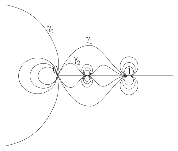
Figure 5. A few preimages of $\gamma$ under the iteration of $K$ (Proposition 3.30).

Proof.

For a postcritical point $z=K^{n}(-1)$, $n\geq 0$,

$$\operatorname{Re}(\phi_{A}(z))=\operatorname{Re}(\phi_{A}(K^{n}(-1))=\operatorname{Re}(\phi_{A}(-1))+n\neq\alpha,$$

by the condition (3.8) on $\alpha$. Hence, the postcritical set does not intersect $\gamma$, so $K^{n}$ is a strict cover of degree $2^{n}$ over $\gamma$, i.e., $(K^{n})^{-1}\gamma$ has $2^{n}$ components, each of which is a smooth open arc. Since $\gamma$ starts from and ends at $0$, each component starts from and ends at a preimage – of order $\leq n$ – of $0$.

Since $K$ commutes with complex conjugation, $\operatorname{Re}(\phi_{A}(\overline{z}))=\operatorname{Re}(\phi_{A}(z))$. Hence, the image of $P$ under complex conjugation – which is again a petal – is mapped by $\phi_{A}$ to the same right half-plane as $P$, so $P$ is invariant under complex conjugation, so its boundary $\gamma$ is also invariant. Again using the fact that $K$ commutes with complex conjugation, the preimage under $K^{n}$ of $\gamma$ is invariant, so the complex conjugate of each component arc is a component arc.

To show that preimages of $\gamma$ do not intersect ${\mathbb{R}}$: It is easy to show, using the estimate $\phi_{A}(z)\approx-1/z$, that $x\mapsto\operatorname{Re}(\phi_{A}(x))$ is strictly increasing for $x$ small and negative. Using $\phi_{A}(x)=\phi_{A}(K^{n}(x))-n$, and the fact that all iterates $K^{n}$ are strictly increasing on $(-1,0)$, we see that $\operatorname{Re}(\phi_{A}(x))$ is strictly increasing on all of $(-1,0)$. On the other hand, $K$ is strictly decreasing on $(-\infty,-1)$ and maps this interval onto $(-1/4,0)$, so – again applying $\phi_{A}(x)=\phi_{A}(K(x))-1$ – $\operatorname{Re}(\phi_{A}(x))$ is strictly decreasing on $(-\infty,-1)$. In particular:

$$\operatorname{Re}(\phi_{A}(x))\geq\operatorname{Re}(\phi_{A}(-1))\quad\text{for $x\in(-\infty,0)$.}$$

If $K^{n}(z)\in\gamma$ (with $n>0$),

$$\begin{split}\operatorname{Re}(\phi_{A}(z))&=\operatorname{Re}(\phi_{A}(K^{n}(z)))-n=\alpha-n\\ &\leq\alpha-1<\operatorname{Re}(\phi_{A}(-1))=\min_{x<0}\operatorname{Re}(\phi_{A}(x)).\end{split}$$

Thus, the preimage under $K^{n}$ of $\gamma$ does not intersect the negative real axis. Since $\gamma$ does not intersect $[0,\infty]$, which is fully invariant, the preimage does not intersect it either, and hence does not intersect ${\mathbb{R}}$.

By condition (3.8) on $\alpha$, the critical value $-1/4$ of $K$ is in $P$, so the Jordan curve made by appending $0$ to $\gamma$ – the boundary of $P$ – runs once around the critical value. Hence, lifts of $\gamma$ under $K$ do not close. One of the two lifts starts at $0$; it cannot end at $0$ and so must end at $\infty$, which is the other preimage of $0$. Since this lift starts in the upper half-plane and, by assertion (2), does not intersect the real axis, it must lie in the upper half-plane ∎

We denote by

• $\gamma_{0}$ the component of $K^{-1}\gamma$ starting at $0$, i.e., the component in the upper half-plane

• $\gamma_{1}$ the component of $K^{-1}\gamma_{0}$ which begins at $0$. Then $\gamma_{1}$ also lies in the upper half-plane and ends at $1$, the preimage of $\infty$

• $\gamma_{2}$ the component of $K^{-1}\gamma_{1}$ which starts at $0$. Again, $\gamma_{2}$ lies in the upper half-plane; it ends at the unique preimage $x_{2}$ of $1$ in $(0,1)$, whose value can easily be computed to be $(3-\sqrt{5})/2$.

Then $\{0\}\cup\gamma_{1}\cup\{1\}\cup\overline{\gamma_{1}}$ is a Jordan curve; we denote its interior by $P_{R}$.

Lemma 3.31.

$P_{R}$ is an attracting petal for $K^{-1}$.

Proof.

Since

• $\partial(K^{-1}P_{R})=K^{-1}(\partial P_{R})=\{0\}\cup\gamma_{2}\cup\{x_{2}\}\cup\overline{\gamma_{2}};$

• $x_{2}\in(0,1)\subset P_{R}$

• $\gamma_{2}\cup\overline{\gamma}_{2}$ does not intersect $\partial P$,

it follows that the closure of $K^{-1}P_{R}$ is contained in $P_{R}\cup\{0\}$. By local theory, $\gamma_{1}$ is tangent to the imaginary axis at $0$; from this it follows that every $K^{-1}$-orbit with initial point not in $(-\infty,0]$ is eventually in $P_{R}$.

It remains only to verify condition (4) of Definition 2.1. We showed above – using Vitali’s theorem – that $(K^{-1})^{n}$ converges uniformly to $0$ on compact subsets of ${\mathbb{C}}\setminus(-\infty,0]$. Since $\partial P_{R}$ is tangent to the imaginary axis at $0$, it follows from local theory that $(K^{-1})^{n}$ converges uniformly to $0$ on the intersection of $P_{R}$ with a sufficiently small disk centered at $0$; uniform convergence on all of $P_{R}$ follows. ∎

Note the mixed character of $P_{R}$: although it is a repelling petal, its boundary is defined as a curve of constant $\operatorname{Re}(\phi_{A})$, except at the two points $0$ and $x_{2}$, where the $\phi_{A}$ is not defined.

By Proposition 2.10, $C_{R}:=P_{R}\setminus K(P_{R})$ projects bijectively to the repelling cylinder ${\cal C}_{R}$ and hence is mapped bijectively by $\operatorname{ixp}\circ\phi_{R}$ to the punctured plane ${\mathbb{C}}\setminus\{0\}$. We write $C^{+}_{R}$ and $C^{-}_{R}$ for the intersections of $C_{R}$ with the open upper and lower half-planes respectively; then

$$C_{R}=C^{+}_{R}\cup(x_{2},1)\cup C^{-}_{R}.$$

$\operatorname{ixp}\circ\phi_{A}$ is analytic on $C^{+}_{R}$ and on $C^{-}_{R}$ but cannot be continued analytically through any point of $(x_{2},1)$. Thus, the image under $\operatorname{ixp}\circ\phi_{R}$ of $C^{+}_{R}$ (respectively $C^{-}_{R}$) is $W^{+}$ (respectively $W^{-}$.) By an argument given above for $\phi_{A}$,

$$\phi_{R}(\overline{z})=\overline{\phi_{R}(z)}+c\quad\text{with $c$ a pure imaginary constant.}$$

so the imaginary part of $\phi_{R}$ is constant on $(0,\infty)$, so $\operatorname{ixp}\circ\phi_{R}$ maps $[r_{2},1]$ to a circle centered at the origin. We chose the real part of the additive constant in $\phi_{R}$ so that $\phi_{R}$ is real on $(0,\infty)$; then

$$W^{+}={\mathbb{D}}\setminus\{0\}\quad\text{and}\quad W^{-}={\mathbb{C}}\setminus\overline{{\mathbb{D}}}.$$

We now have all the pieces in place to prove that the only asymptotic values of ${\mathbf{k}}$ are $0$ and $\infty$. We assume that $s\mapsto\tau(s),s\in[0,1)$ is a continuous arc in $W^{+}$ converging to the unit circle as $s\to 1$ (but not necessarily to an particular point of the circle) such that ${\mathbf{k}}(\tau(s))$ converges as $s\to 1$ to a finite nonzero value $z_{\infty}$, and we show this leads to a contradiction. We select an $\alpha$ as in (3.8) and also so that

$$\frac{1}{2\pi}\operatorname{Arg}(z_{\infty})-\alpha\notin{\mathbb{Z}}.$$

Since ${\mathbf{k}}(\tau(s))\to z_{\infty}$, we can – by deleting an initial segment of $\tau$ and reparametrizing – assume that

(3.9) $$\frac{1}{2\pi}\operatorname{Arg}(H(\tau(s))-\alpha\notin{\mathbb{Z}}\quad\text{for $0\leq s<1$.}$$

Recall that $\operatorname{ixp}\circ\phi_{R}$ maps $C^{+}_{R}$ bijectively to $W^{+}$. We denote by $\hat{\tau}(s)$ the image of $\tau(s)$ under the inverse of this bijection. We claim that the lift $\hat{\tau}(\,.\,)$ is continuous. To see this, we note that

$${\mathbf{k}}(\tau(s))=\exp(2\pi i\phi_{A}(\hat{\tau}(s))),$$

so, by (3.9).

(3.10) $$\operatorname{Re}(\phi_{A}(\hat{\tau}(s)))-\alpha\notin{\mathbb{Z}}\quad\text{for $0\leq s<1$,}$$

that is, the values of $\hat{\tau}(s)$ lie in the interior of $P^{+}_{R}$, not on the “edges”. Since $\operatorname{ixp}\circ\phi_{R}$ is a local homeomorphism everywhere in the interior of $C^{+}_{R}$, continuity of $\hat{\tau}(s)$ follows.

We recall that $P$ denotes here the attracting petal mapped by $\phi_{A}$ to the half-plane $\{\operatorname{Re}(w)>\alpha\}$. Since the orbit of the initial point $\hat{\tau}(0)$ of the lift is eventually in $P$, and since $\operatorname{Re}(\phi_{A}(\hat{\tau}(0))-\alpha\notin{\mathbb{Z}}$, there exist positive integers $n$ and $m$ since that

$$K^{n}(\hat{\tau}(0))\in C:=\{z\in P:\alpha+m<\operatorname{Re}(\phi_{A}(z))<\alpha+m+1\}$$

Because of (3.10), $\hat{\tau}(s)$ never intersects either boundary arc of the crescent $C$, so, by continuity,

$$\tilde{\tau}(s):=K^{n}(\hat{\tau}(s))\in C\quad\text{for $0\leq s<1$.}$$

Because the base arc $\tau(s)$ (in $W^{+}$) approaches the unit circle as $s\to 1$, $\hat{\tau}(s)$ approaches $[x_{2},1]$, so, because $[0,\infty]$ is mapped to itself by $K$, $\tilde{\tau}(s)$ approaches $[0,\infty]$ as $s\to 1$. We thus have the following situation:

1. $s\mapsto\tilde{\tau}(s)$ is a continuous arc in the crescent $C$.

2. $s\mapsto\tilde{\tau}(s)$ approaches $[0,\infty]$ as $s\to 1$.

3. $\operatorname{ixp}(\phi_{A}(\tilde{\tau}(s)))$ approaches a finite non-zero limit $z_{0}$ as $s\to 1$.

It is now easy to show that these three assertions lead to a contradiction. We first argue that (1) and (2) imply

(3.11) $$|\operatorname{Im}(\phi_{A}(\tilde{\tau}(s)))|\to\infty.$$

Then ${\mathbf{k}}(\tau(s))=\exp(2\pi i\phi_{A}(\tilde{\tau})(s))$ converges to $0$ (if $\operatorname{Im}(\phi_{A}(\tilde{\tau})(s))\to+\infty$) or to $\infty$, contradicting (3).

To prove (3.11): for sufficiently small positive $\epsilon$, there is an attracting petal $P_{\epsilon}$ mapped homeomorphically by $\phi_{A}$ to the half-plane $\{\operatorname{Im}(w)>\alpha-\epsilon\}$. Let $r$ be a positive real number and let $R_{r}$ denote the preimage under the restriction of $\phi_{A}$ to such a $P_{\epsilon}$ of the compact rectangle

$$\{u+iv:\alpha+m\leq u\leq\alpha+m+1,-r\leq v\leq r\}$$

Since $R_{r}$ is compact and disjoint from $[0,\infty]$, its distance from $[0,\infty]$ is strictly positive. By (1), if $|\operatorname{Im}(\phi_{A}(\tilde{\tau}(s))|\leq r$, then $\tilde{\tau}(s)\in R_{r}$. Hence, by (2), $|\operatorname{Im}(\phi_{A}(\tilde{\tau}(s))|$ is eventually $>r$. Since this is true for all $r$, (3.11) holds.

It is evident that $\{0,\infty\}\subset\operatorname{Asym}(H)$. Indeed, for small enough $\epsilon>0$ the projection of $\gamma_{1}\cap D_{\epsilon}(1)$ by $\operatorname{ixp}\circ\phi_{R}$ is a simple curve in ${\mathbb{D}}$ whose image under $H$ lands at $0$; similarly $\gamma_{2}$ yields a curve whose image under $H$ lands at $\infty$.

Now let

$$\tau:[0,1)\to{\mathbb{D}}=\operatorname{Dom}(H)$$

be a curve such that $\tau(t)$ converges to the unit circle ${\mathbb{T}}$ as $t\to 1-$. Let

$$\tilde{\tau}:[0,1)\subset\hat{\mathbb{C}}\setminus{\mathbb{R}}_{\geq 0}$$

be a component of its lift under $\operatorname{ixp}\circ\phi_{R}$, parametrized so that

(3.12) $$\tilde{\tau}(t)\to{\mathbb{R}}_{\geq 0}\text{ as }t\to 1-.$$

Let $C^{\prime}$ be a connected component of $K^{n}(C)$ for $n\in{\mathbb{Z}}$. We will say that the curve $\tilde{\tau}$ crosses $C^{\prime}$ if there exist $t_{1}\neq t_{2}\in(0,1)$ and $n\in{\mathbb{Z}}$ such that

$$\tilde{\tau}:(t_{1},t_{2})\to C^{\prime},\;K^{n}(\tilde{\tau}(t_{1}))\in\gamma,\text{ and }K^{n}(\tilde{\tau}(t_{2}))\in h(\gamma).$$

Note that every time $\tilde{\tau}$ crosses some $C^{\prime}$, the image ${\mathbf{k}}(\tau)$ winds once around the cylinder ${\mathbb{C}}/{\mathbb{Z}}\simeq\hat{\mathbb{C}}\setminus\{0,\infty\}$. Hence, we have the following two possibilities:

1. $\tilde{\tau}$ crosses finitely many connected components of $\cup_{n\in{\mathbb{Z}}}K^{n}(C)$;

2. $\lim_{t\to 1-}{\mathbf{k}}(\tau(t))\in\{0,\infty\}.$

In case (2), we are done.

Standard considerations of dynamics on $J(K)$ imply that for every $x\in{\mathbb{R}}_{\geq 0}$ which is not a preimage of $0$, there exists an infinite sequence of cross-cuts $l_{k}\equiv K^{-{n_{k}}}(\gamma_{i})$ for some choice of the inverse branch and $i=1,2$ such that denoting $N_{k}$ the cross-cut neighborhood of $l_{k}$ in $\hat{\mathbb{C}}\setminus{\mathbb{R}}_{\geq 0}$, we have

$$\overline{N_{k}}\cap{\mathbb{R}}\ni\{x\}.$$

In view of (1) and (2) this implies that $x$ cannot be accumulated by $\tilde{\tau}$. Since points $x$ as above form a dense set on ${\mathbb{R}}_{\geq 0}$, we see that there exists a limit

$$s=\lim_{t\to 1-}\tilde{\tau}(t)\text{ and }s\in\cup K^{-n}(0).$$

In view of (1), this implies that

$$\lim_{t\to 1-}{\mathbf{k}}(\tau(t))\in\{0,\infty\}.$$

∎

3.5. Parabolic renormalization of $f_{0}$

We now have:

Proposition 3.32.

The maps $f_{0}$ and $K$ are both renormalizable.

Proof.

The arguments are identical, so we only argue for $f_{0}$. Let us replace ${\mathbf{h}}_{f_{0}}$ by $c{\mathbf{h}}_{f_{0}}$ if needed so that ${\mathbf{h}}^{\prime}_{f_{0}}(0)=1$. We have to show that the coefficient $a$ in the Taylor expansion

$${\mathbf{h}}_{f_{0}}(z)=z+az^{2}+\cdots$$

is not equal to $0$, or, in other words, that $z=0$ is a simple parabolic point of ${\mathbf{h}}_{f_{0}}$. Let $P_{0}$ be an attracting petal of $z=0$. For $n\geq 1$ denote $P_{-n}$ the component of the preimage $({\mathbf{h}}_{f_{0}})^{-1}(P_{-(n-1)})$ which contains $P_{-(n-1)}$. We claim that there exists $n$ such that $P_{-n}$ contains the unique critical value $v$ of ${\mathbf{h}}_{f_{0}}$. Assume the contrary. Then for every $n$ the domain $P_{-n}$ is a topological disk. Denote

$$B_{0}=\cup P_{-n}\subset\hat{W}^{+}.$$

The Fatou coordinate $\phi_{A}$ of ${\mathbf{h}}_{f_{0}}$ extends to all of $B_{0}$ via the functional equation

$$\phi_{A}\circ{\mathbf{h}}_{f_{0}}(z)=\phi_{A}(z)+1$$

as an unbranched analytic map. It is trivial to see that its image is the whole complex plane ${\mathbb{C}}$, and hence $U$ must be a parabolic domain. This is impossible, however, as $U$ is a subset of a Jordan domain $\hat{W}^{+}\subset{\mathbb{C}}$.

Now assume that $a=0$. Then the parabolic point $z=0$ has at least two distinct attracting directions $v_{1},v_{2}\in S^{1}$. Consider corresponding attracting petals $P_{A}^{1}\cap P_{A}^{2}=\emptyset$. As we have shown above, the critical value $v$ must be contained in the intersection of their preimages. This leads to a contradiction, as in this case

$$\lim{\mathbf{h}}_{f_{0}}^{n}(v)/|{\mathbf{h}}_{f_{0}}^{n}(v)|=v_{1}=v_{2}.$$

∎

We now turn to the dynamics of the parabolic renormalization

$$F\equiv{\cal P}(f_{0}):\hat{W}^{+}\to\hat{\mathbb{C}}.$$

Definition 3.3.

The points $z\in\hat{W}^{+}$ whose orbits do not escape $\hat{W}^{+}$ form the filled Julia set $K(F)$. Its boundary $J(F)$ is the Julia set.

Lavaurs [Lav] has shown that

Theorem 3.33 ([Lav]).

The interior of the filled Julia set $K(F)$ coincides with the basin of the parabolic point $0$. Repelling periodic orbits of $F$ are contained in $J(F)$ and are dense in $J(F)$.

Let $P^{0}\equiv P_{A}$ be an attracting petal of $F$. For $n\in{\mathbb{N}}$ inductively define $P^{-n}$ to be the connected component of the inverse image $F^{-1}(P^{-(n-1)})$ which contains $P^{-(n-1)}$. The same considerations as in the proof of Proposition 3.32 imply:

Proposition 3.34.

There exists $n\in{\mathbb{N}}$ such that $P^{-n}$ is a topological disk which contains $v$ in its closure.

3.6. A note on the general theory for analytic maps of finite type

As the previous example clearly demonstrates, when $f$ has global covering properties, we can expect the Écale-Voronin map ${\cal E}_{f}$ to also possess a well-understood global covering structure. The appropriate setting for a global structure theory for Écalle-Voronin maps is that of analytic maps of finite type, developed in A. Epstein’s thesis [Ep]. While we will not need these results in our investigation, we will briefly mention some of them below for the sake of completeness of the exposition.

Definition 3.4 ([Ep]).

Let $f:W\to X$ be an analytic map between two Riemann surfaces. Assume further that $X$ is compact, and $W$ lies in some compact surface $Y$. Suppose that $f$ is nowhere constant, and that every isolated singularity of $f$ is essential. We say that $f$ is a map of finite type if $\operatorname{Sing}(f)$ is a finite set.

Rational endomorphisms $f:\hat{\mathbb{C}}\to\hat{\mathbb{C}}$ are obviously maps of finite type. Epstein demonstrated:

Theorem 3.35.

[Ep] If an analytic map $f$ with a parabolic cycle is of finite type, then the corresponding Écalle-Voronin maps ${\cal E}_{f}:W_{f}\to\hat{\mathbb{C}}$ inherit the same property.

Epstein further showed that the familiar properties, such as density of repelling periodic points and topological minimality, hold for Julia sets of analytic dynamical systems of finite type. Most importantly, he proved that the Fatou-Sullivan structure theory holds for the Fatou sets of such dynamical systems:

Theorem 3.36.

[Ep] Every connected component of the Fatou set of a map of finite type is pre-periodic. All periodic Fatou components are either basins (attracting or parabolic), or rotation domains (Siegel disks or Herman rings).

4. A class of analytic mappings invariant under ${\cal P}$

4.1. Definition of ${{{{\mathbf{P}}}}_{0}}$

We will now specialize to a much narrower class of analytic maps with parabolic orbits. As before, we write

$$f_{0}(z)=z+z^{2},$$

and we set

$$F\equiv{\cal P}(f_{0})\text{ and }W_{F}=\operatorname{Dom}({\cal P}(f_{0})).$$

Definition 4.1.

We will denote $\widetilde{{{{\mathbf{P}}}}}$ the class of analytic germs $f(z)$ at the origin which have maximal analytic extensions

$$f:{\cal D}(f)\to\hat{\mathbb{C}}$$

such that

• ${\cal D}(f)$ is a simply-connected domain;

• Denoting $\varphi_{f}$ the Riemann mapping

  $$\varphi_{f}:{\mathbb{D}}\to{\cal D}(f),\text{ with }\varphi_{f}(0)=0\text{ and }\varphi^{\prime}_{f}(0)>0,$$

  we have

  $$f\circ\varphi_{f}(z)=v\cdot F\circ\varphi_{F}(e^{2\pi i\theta}z),\text{ for }v\neq 0,\;\theta\in{\mathbb{R}}.$$

Note that denoting $c$ and $c^{F}$ the unique critical values of $f$ and $F={\cal P}(f_{0})$ respectively, we get the rescaling factor as $v=c/c^{F}$.

If we again let ${\mathbf{k}}$ be the normalized ${\mathbf{h}}_{K}$ for the Koebe function $K(z)$, then, by Proposition 3.25, the property (II) in the above definition is equivalent to

• Denoting $\varphi_{f}$ the Riemann mapping

  $$\varphi_{f}:{\mathbb{D}}\to{\cal D}(f),\text{ with }\varphi_{f}(0)=0\text{ and }\varphi^{\prime}_{f}(0)>0,$$

  we have

  $$f\circ\varphi_{f}(z)=v\cdot{\mathbf{k}}(e^{2\pi i\theta}z),\text{ for }v\neq 0,\;\theta\in{\mathbb{R}}.$$

We note:

Proposition 4.1.

For all $f\in\widetilde{{{{\mathbf{P}}}}}$ we have $f^{\prime\prime}(0)\neq 0$.

Proof.

Suppose $f^{\prime\prime}(0)=0$. By multiplying by a non-zero constant, if necessary, we may reduce the proof to the case when $f^{\prime}(0)=1$, so that $f(z)=z+az^{n}+\cdots$ for $n>2$. A Leau-Fatou flower of $f$ has $n-1\geq 2$ attracting petals. Since $f$ has a single critical value $c^{f}$, there exists an ample petal $P_{A}$ such that

$$P_{A}\cap\cup_{k\in{\mathbb{N}}}f^{k}(c^{f})=\emptyset.$$

Let $\phi_{A}$ be an attracting Fatou coordinate defined on $P_{A}$. Set $P_{0}\equiv P_{A}$ and inductively define $P_{-n}$ as the component of the preimage $f^{-1}(P_{-(n-1)})$ which contains $P_{-(n-1)}$ for $n\in{\mathbb{N}}$. The function $\phi_{A}$ analytically extends via the functional equation

$$\phi_{A}\circ f(z)=\phi_{A}(z)+1$$

to the union

$$U\equiv\cup P_{-n}\subset\operatorname{Dom}(f).$$

A simple induction shows that $\phi_{A}$ is univalent on $P_{-n}$, and hence on all of $U$. On the other hand, $\phi_{A}(U)={\mathbb{C}}$, which is impossible since $U$ is a hyperbolic domain. ∎

Definition 4.2.

We define $\widehat{{{{\mathbf{P}}}}}$ as the set of maps $f\in\widetilde{{{{\mathbf{P}}}}}$ of the form

$$f(z)=z+z^{2}+\cdots$$

at the origin.

We further define ${{{{\mathbf{P}}}}}\subset\widehat{{{{\mathbf{P}}}}}$ as the collection of maps $f\in\widehat{{{{\mathbf{P}}}}}$ such that the domain ${\cal D}(f)$ has locally connected boundary. Finally, ${{{{\mathbf{P}}}}_{0}}\subset{{{{\mathbf{P}}}}}$ consists of maps whose domain of definition is Jordan.

Since $F={\cal P}(f_{0})\in{{{{\mathbf{P}}}}_{0}}$, we have

Proposition 4.2.

The class ${{{{\mathbf{P}}}}_{0}}$ is non-empty.

We now set out to prove the following theorem:

Theorem 4.3.

Every $f\in{{{{\mathbf{P}}}}_{0}}$ is renormalizable, and the parabolic renormalization ${\cal P}(f)\in{{{{\mathbf{P}}}}_{0}}$.

Let $f\in\widetilde{{{{\mathbf{P}}}}}$ and let $P_{0}$ be an attracting petal of the parabolic point $z=0$. For $n\geq 1$ let $P_{-n}$ be the component of $f^{-1}(P_{-(n-1)})$ which contains $P_{-(n-1)}$. We let

$$B_{0}^{f}\equiv\cup P_{-n},$$

and call it the immediate basin of $0$. We note:

Proposition 4.4.

For $f\in\widetilde{{{{\mathbf{P}}}}}$ the unique critical value $c^{f}\in B_{0}^{f}$. Moreover, there exists an attracting petal $P_{A}\subset B_{0}^{f}$ which is a topological disk containing $c^{f}$ in its interior.

Proof.

Assume that $v\notin B_{0}^{f}$. The attracting Fatou coordinate $\phi_{A}^{f}$ extends from $P_{0}$ to the whole of $B_{0}^{f}$ via the functional equation

$$\phi_{A}^{f}\circ f(z)=\phi_{A}^{f}(z)+1.$$

A simple induction shows that $P_{-n}$ is an increasing sequence of topological disks, on each of which $\phi_{A}$ is univalent. Hence, $\phi_{A}$ restricted to $B_{0}^{f}$ is a conformal homeomorphism onto the image. Yet it is clear that the image of $\phi_{A}$ restricted to $B_{0}^{f}$ is the whole of ${\mathbb{C}}$, which contradicts the fact that $B_{0}^{f}$ is a hyperbolic domain. The second part of the statement is elementary, and is left to the reader. ∎

Pushing the argument a little further, we have:

Proposition 4.5.

For $f\in\widetilde{{{{\mathbf{P}}}}}$ the immediate basin $B_{0}^{f}$ is simply connected and contains exactly one critical point of $f$. The restriction $f:B_{0}^{f}\to B_{0}^{f}$ is a degree-$2$ branched covering.

Proof.

By Proposition 4.4, there exists $n$ such that $P_{-n}$ contains the critical value $c^{f}$. Inductively applying Lemma 3.7, we see that for $k\in{\mathbb{N}}$ the domain $P_{-(n+k)}$ is a topological disk, and $f:P_{-(n+k)}\to P_{-(n+k-1)}$ is a branched covering of degree $2$ with a single, simple critical point. ∎

The proof of Theorem 4.3 will rely on the following key result, which is a direct analogue of Theorem 3.10.

Theorem 4.6.

Let $f\in{{{{\mathbf{P}}}}_{0}}$, and denote $B^{0}_{f}$ the immediate basin of the parabolic point $0$ of $f$. Then $B_{f}^{0}$ is a Jordan domain. Denote $\hat{f}$ the continuous extension of $f$ to $\partial B_{0}^{f}$. There exists a homeomorphism $\rho:\partial B_{0}^{f}\to{\mathbb{T}}$ such that

$$\rho(\hat{f}(z))=2\rho(z)\operatorname{mod}1.$$

The proof of Theorem 4.6 is quite involved, as it will require a detailed understanding of the covering properties of a map in ${{{{\mathbf{P}}}}_{0}}$. Let us show how Theorem 4.6 implies Theorem 4.3:

Proof.

Consider a Riemann map

$$v:{\mathbb{D}}\to B^{f}_{0}$$

which maps $0$ to the sole critical point of $f$ inside $B^{f}_{0}$. By Theorem 4.6 and Carathéodory Theorem, the Riemann map has a continuous extension to a homeomorphism $\tilde{v}:\overline{{\mathbb{D}}}\to\overline{B^{f}_{0}}$.

Let us further normalize the Riemann map ${\mathbb{D}}\to B^{f}_{0}$ by requiring that $\tilde{v}(1)=0.$ This specifies the mapping uniquely, and we denote it $\psi_{f}$.

By Theorem 2.33,

$$(\psi_{f})^{-1}\circ f\circ\psi_{f}=B:{\mathbb{D}}\to{\mathbb{D}}\text{, where }B(z)=\frac{3z^{2}+1}{3+z^{2}}.$$

Let us set

$$\chi=\psi_{f_{0}}\circ(\psi_{f})^{-1}:B_{0}^{f}\mapsto B_{0}^{f_{0}}.$$

By the discussion above, this mapping is a conjugacy:

$$\chi\circ f|_{B_{0}}=f_{0}\circ\chi|_{B_{0}}.$$

Let us fix

$$D=\{|w|<|c^{f}|\},$$

and let $g$ be the branch of $f^{-1}$ fixing $0$ which is defined in $D$. For the moment, the map ${\cal P}_{f}$ is only defined locally in a neighborhood of $0$, which is a priori dependent on the choice of a repelling petal $P_{R}^{f}$. Let us fix a petal $P_{R}^{f}\subset D$.

The map $F={\cal P}(f_{0})$ has a maximal extension to a Jordan domain $W_{F}$. Let us use Theorem 3.10 to select a simple arc $\gamma$ connecting $0$ with $a\in J_{f_{0}}$ inside $B_{0}^{f_{0}}\cap P_{R}^{f_{0}}$ in some repelling petal of $f_{0}$, such that:

• ${\gamma}\cap J_{f_{0}}=\{a\}$;

• $\gamma\cap f_{0}(\gamma)=\{0\}$;

• denoting $V_{0}\subset P_{R}^{f_{0}}$ the Jordan domain bounded by $\gamma$, $f_{0}(\gamma)$, and the Jordan subarc of $J_{f_{0}}$ between $a$ and $f_{0}(a)$, we have a one-to-one correspondence between points in $W_{f_{0}}$ and points in

  $$\hat{V}_{0}\equiv(V_{0}\cup\gamma)\setminus\{a\};$$

• $\hat{V}\equiv\chi(\hat{V}_{0})\subset P_{R}^{f}$.

Denote ${\cal W}\subset{\cal C}_{R}^{f}$ the quotient of $\hat{V}$ by the action of $f$. Let $W\subset{\mathbb{C}}$ be the image of ${\cal W}$ by $\operatorname{ixp}\circ\phi_{R}^{f}$ with the puncture at $0$ filled. By construction, $W$ is a Jordan domain, which contains a neighborhood of $0$. We claim that:

1. the germ ${\cal P}(f)$ analytically continues to all of $W$, and, moreover,

2. ${\cal P}(f)$ cannot be analytically continued to a neighborhood of any point $z\in\partial W$.

Since $V\subset P_{R}^{f}\cap B_{0}^{f}$, the first statement is immediate by the definition of ${\cal P}(f)$. Furthermore, by (3.1), the set of critical points

$$\text{Crit}(\phi^{f}_{A})=\chi(\text{Crit}(\phi^{f_{0}}_{A}))$$

contains $\partial B_{0}^{f}$ in its closure. Since $\partial W$ is a projection of a Jordan subarc of $\partial B_{0}^{f}$, this implies (2). We have thus shown the existence of a Jordan domain

$$\operatorname{Dom}(f)=W.$$

Let

$$\varphi_{f}:\operatorname{Dom}(f)\to{\mathbb{D}}$$

be the unique Riemann mapping normalized as in Definition (4.1). The uniqueness of the Riemann mapping implies that, up to a pre-composition with a rotation, it is given by the composition

$$\operatorname{ixp}\circ\phi_{R}^{f}\circ\chi^{-1}\circ(\phi_{R}^{f_{0}})^{-1}\circ\operatorname{ixp}^{-1}\circ\varphi_{F},$$

with suitably chosen inverse branches.

The map $\chi$ induces a conformal isomorphism between attracting Fatou cylinders ${\cal C}^{f}_{A}\to{\cal C}^{f_{0}}_{A}$. After uniformizing the cylinders by ${\mathbb{C}}^{*}$, it takes the form

$$\tau\equiv\operatorname{ixp}\circ\phi_{A}^{f_{0}}\circ\chi\circ(\phi_{A}^{f})^{-1}\circ\operatorname{ixp}^{-1}:{\mathbb{C}}^{*}\to{\mathbb{C}}^{*}$$

(with suitably chosen inverse branches). By Proposition 2.12, $\tau$ is a multiplication by a non-zero constant.

A diagram chase now implies that

$${\cal P}_{f}\circ\varphi_{f}(z)=v\cdot F\circ\varphi_{F}(e^{2\pi i\theta}z)$$

for some $v\neq 0$ and $\theta\in{\mathbb{R}}$. Since the unique critical value of the mapping on the left coincides with that of the mapping on the right, $v=c^{{\cal P}(f)}/c^{F}$.

∎

Let $f\in{{{{\mathbf{P}}}}_{0}}$. By definition of parabolic renormalization, for any repelling petal $P_{R}^{f}$ the projection of the intersection $P_{R}^{f}\cap B_{0}^{f}$ by $\operatorname{ixp}\circ\phi_{R}^{f}$ lies in the domain $\operatorname{Dom}({\cal P}(f))$. We remark, that it covers all of it:

Remark 4.1.

For any choice of $P_{R}^{f}$, the projection

$$\operatorname{ixp}\circ\phi_{R}^{f}(P_{R}^{f}\cap B_{0}^{f})\cup\{0,\infty\}$$

is a union of two disjoint Jordan domains $W^{+}\ni 0$ and $W^{-}\ni\infty$ with

$$W^{+}=\operatorname{Dom}({\cal P}(f)).$$

We begin the proof with a lemma:

Lemma 4.7.

Let $D$ be a Jordan domain containing $0$ such that

• $c^{f}\notin D$;

• there exists a Jordan arc $\tau\ni c^{f}$ in $\hat{\mathbb{C}}\setminus D$ running to $\infty$ such that $\tau\cap B^{f}_{0}$ is connected.

Analytically extend $g$ to $D$. If $w\in B^{f}_{0}\cap D$, then $g(w)\in B^{f}_{0}$.

Proof.

Standard considerations imply that $g$ extends to a branch $\hat{g}$ of $f^{-1}$ defined and analytic on ${\mathbb{C}}\setminus\tau$. Note that $B^{f}_{0}\setminus\tau$ is also connected. For a point $z_{0}$ on the negative real axis and near to $0$, the asymptotic development for the attracting Fatou coordinate (Proposition 2.6) implies that $z_{0}$ and $g(z_{0})\approx z_{0}$ both lie in $B_{0}^{f}$.

Let $z\in B^{f}_{0}\setminus\tau$; then there is a Jordan arc $\gamma$ in $B^{f}_{0}\setminus\tau$ from $z_{0}$ to $z$. By the covering properties of $f$, there is a unique lift $\tilde{\gamma}$ of $\gamma$ starting at $g(z_{0})$. Furthermore, this lift is contained in $B^{f}_{0}$, so its end point is in $B^{f}_{0}$. On the other hand, for $\hat{g}$ as above,

$$s\mapsto\hat{g}(\gamma(s))$$

is another lift with the same starting point. By uniqueness of lifts, it coincides with $\tilde{\gamma}$. In particular, the end point of $\tilde{\gamma}$ is $\hat{g}(z)$. Since we already know that $\tilde{\gamma}$ lies in $B^{f}_{0}$, it follows that $\hat{g}(z)\in B^{f}_{0}$. In particular, if $z\in D$, then $\hat{g}(z)=g(z)$, so $g(z)\in B^{f}_{0}$, as asserted. ∎

Proof of Remark 4.1.

Extend the local inverse $g$ to all of $P_{R}^{f}$. If necessary, replace $P_{R}^{f}$ with $g^{n}(P_{R}^{f})$ for a sufficienly large $n\in{\mathbb{N}}$ to guarantee that there exists a domain $D$ as described in Lemma 4.7 such that $P_{R}^{f}\subset D$.

Denote

$$W=\operatorname{ixp}\circ\phi_{R}^{f}(P_{R}^{f}\cap B_{0}^{f})\text{ and }V=\operatorname{ixp}\circ\phi_{R}^{f}(P_{R}^{f}\setminus B_{0}^{f}).$$

Lemma 4.7 implies that $W$ and $V$ are disjoint. The common boundary $J=\partial W=\partial V$ is the projection

$$J=\operatorname{ixp}\circ\phi_{R}^{f}(P_{R}^{f}\cap\partial B_{0}^{f}).$$

By Theorem 4.6, $J$ is a union of two disjoint Jordan curves. Hence, $W$ is a union of two Jordan domains $W^{+}\ni 0$ and $W^{-}\ni\infty$, bounded by the components of $J$. On the other hand, $\operatorname{Dom}({\cal P}(f))$ is also a Jordan domain, which does not intersect $J$. Hence, it is contained in the component of $W$ which surrounds $0$, and is, in fact, equal to it by the maximality of the analytic continuation of ${\cal P}(f)$. ∎

4.2. The structure of the immediate parabolic basin of a map in ${{{{\mathbf{P}}}}}$

In this section we will prove several results about lifts of parametrized paths of the form

$$s:[0,1]\to\hat{\mathbb{C}}.$$

We will always assume $s(t)$ to be continuous on $(0,1)$. We will say that $s$ lands at a point $a\in\hat{\mathbb{C}}$ if

$$\lim_{t\to b}s(t)=a\text{ for }b\in\{0,1\}.$$

We will generally use the same letter $s$ to denote the function $s(t)$ and the curve $s([0,1])$ which is its range. We will call the image of the open interval $(0,1)$ under $s(t)$ an open path, and will denote it by $\overset{\circ}{s}$. Several times we will encounter the situation when there is a domain $W\subset\hat{\mathbb{C}}$ and a curve

$$s:(0,1)\mapsto{W},$$

which lands at a point $w\in\partial W$ (to fix the ideas, assume that $s(0)=w$). If $w$ has more than one prime end in $W$, then there is a unique prime end $\hat{w}$ such that for every prime end neighborhood $N(\hat{w})$ we have $s\cap N(\hat{w})\neq\emptyset$. In this case, we will write

$$s(t)\underset{t\to 0+}{\longrightarrow}\hat{w}.$$

Let $f\in{{{{\mathbf{P}}}}}$. Let $s\mapsto\gamma(s)$ be a continuous path such that:

• $\gamma(0)=\gamma(1)=0$;

• $\gamma(s)\neq c^{f}$ for all $s\in(0,1)$;

• the winding number $W(\gamma,c^{f})=1$;

• there is an $\epsilon\in(0,\pi/2)$ such that $\gamma\cap D_{\epsilon}(0)$ lies in the sector $\{\text{Arg}(z)\in(-\pi-\epsilon,-\pi+\epsilon)\}$.

Standard path-lifting considerations imply that there exists a unique continuous mapping $s\mapsto\tilde{\gamma}(s)$, defined for $0\leq s<1$ such that

$$\tilde{\gamma}(0)=0,\text{ and }f(\tilde{\gamma}(s))=\gamma(s)\text{ for }0\leq s<1.$$

We claim:

Proposition 4.8.

We have the following.

1. For any loop $\gamma$ as above, there exists a limit

   $$t\in\partial\operatorname{Dom}(f)=\lim_{s\to 1}\tilde{\gamma}(s).$$

2. This point (which we will denote $t^{f}$) is the same for all loops $\gamma$ satisfying the above properties.

3. For $f=F\equiv{\cal P}(f_{0})$, the point $t^{F}$ is the projection of the inverse orbit

   $$z_{-n}=({g_{0}})^{n}(-1)$$

   by $\operatorname{ixp}\circ\phi_{R}$.

4. Similarly, for $f=H\equiv{\cal P}(h)$, the point $t^{H}$ is the projection of the inverse orbit

   $$z_{-n}=K^{-n}(1),$$

   where the inverse branch is selected to preserve the interval $(0,1)$.

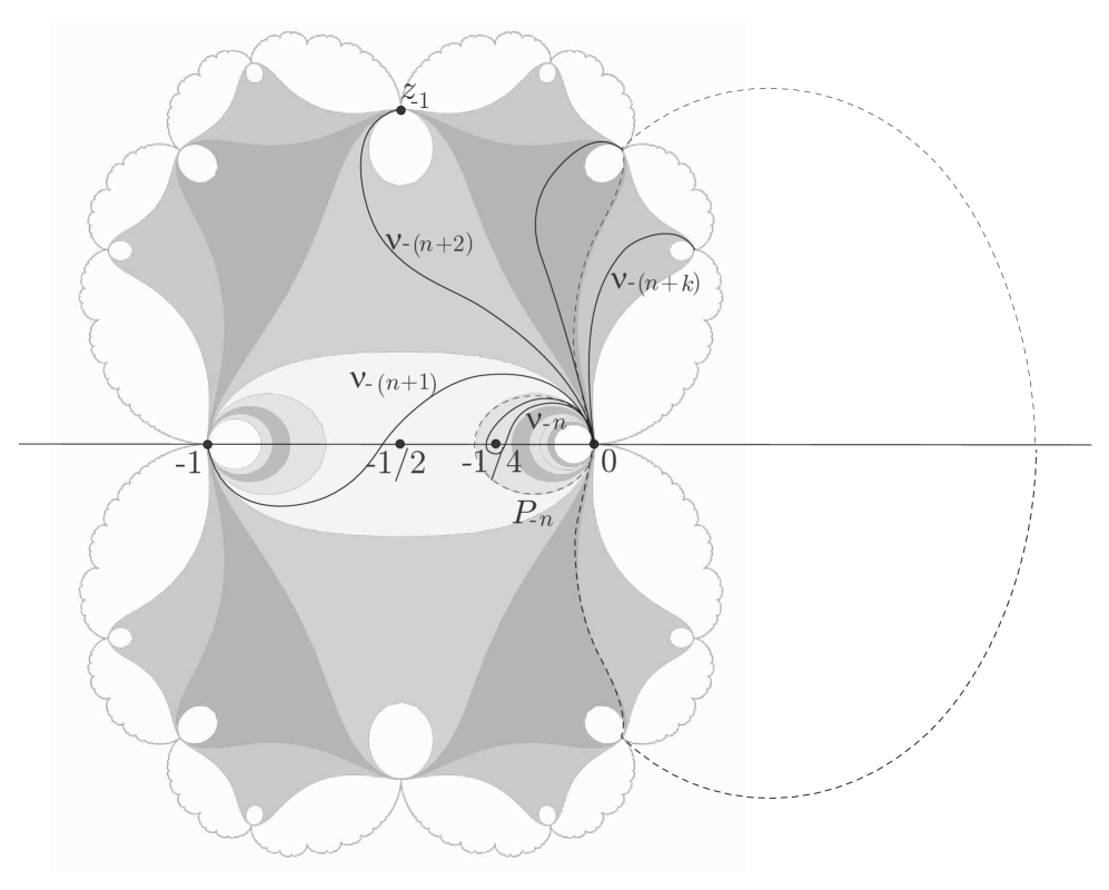
Figure 6. An illustration of the proof of Proposition 4.8

Proof of Proposition 4.8.

We will prove (1) - (3) for $f=F\equiv{\cal P}(f_{0})$. By the definition of ${{{{\mathbf{P}}}}}$ and by Carathéodory Theorem, this will imply (1) and (2) in the general case. The proof of (4) follows along the same lines as the proof of (3) and will be left to the reader.

Let us begin by selecting a simple curve $\sigma\subset\hat{\mathbb{C}}$ which connects $0$ and $\infty$, does not intersect with $\gamma$ except at the endpoint $0$, and such that an analytic branch of the logarithm defined on a neighborhood of $\sigma$ has bounded imaginary part.

Recall that the attracting Fatou coordinate $\phi_{A}^{f_{0}}$ holomorphically extends to the whole immediate basin $B_{0}^{f_{0}}$ via the equation

$$\phi_{A}^{f_{0}}\circ f_{0}(z)=\phi_{A}^{f_{0}}(z)+1.$$

This extension is a branched covering $B_{0}^{f_{0}}\to{\mathbb{C}}$ with simple ramification points at preimages of the critical point $-1/2$.

It is elementary to see what the lift of $\sigma$ to the dynamical plane of $f_{0}$ looks like. We summarize its properties below, and invite the reader to verify them. Let us denote

$$\overset{\circ}{\sigma}\equiv\sigma\setminus\{0,\infty\}.$$

The preimage of $\overset{\circ}{\sigma}$ under $\operatorname{ixp}\circ\phi_{A}^{f_{0}}$ is a countable collection of disjoint simple curves $\cup\overset{\circ}{s_{j}}$. We will denote the closure of $\overset{\circ}{s_{j}}$ by $s_{j}$. It is obtained by adjoining two endpoints to $\overset{\circ}{s}_{j}$: two elements of the grand orbit $\cup_{n\geq 0}(f_{0})^{-n}(0)$, which are not necessarily distinct.

The curves $s_{j}$ form a grand orbit under $f_{0}$ as well. The connected components

$$S_{i}\text{ of }B_{0}^{f_{0}}\setminus\cup s_{j}$$

are mapped by the attracting Fatou coordinate $\phi_{A}^{f_{0}}$ onto curvilinear strips $\tilde{S}_{i}\subset{\mathbb{C}}$ of infinite height and of unit width. The strips $\tilde{S}_{i}$ are bounded by unit translates of the same curve $\tilde{\sigma}\subset{\mathbb{C}}$. Let us enumerate these strips in such a way that

$$T:\tilde{S}_{i}\to\tilde{S}_{i+1},\text{ where }T(z)=z+1.$$

For a fixed $\tilde{S}_{i}$ we have

$$\sup_{x,y\in\tilde{S}_{i}}(\operatorname{Re}(x)-\operatorname{Re}(y))<\infty.$$

This is where we have used the assumption on the branches of $\log$ in $\hat{\mathbb{C}}\setminus\sigma$. Thus for every $\ell\in{\mathbb{Z}}$ the union $\cup_{i\geq\ell}\tilde{S}_{i}$ contains a right half-plane.

Now let us take any component $S_{i}\subset B_{0}^{f_{0}}$. The above observation implies that, for any $\ell\in{\mathbb{N}}$,

$$\phi_{A}^{f_{0}}(\cup_{k\geq\ell}f^{k}(S_{i}))\supset\{\operatorname{Re}z>A\}$$

for some $A\in{\mathbb{R}}$. Note that if $\ell$ is large enough, then $\cup_{k\geq\ell}f^{k}(S_{i})$ does not contain any preimages of $-1/2$, and hence the restriction of $\phi_{A}^{f_{0}}$ to it is unbranched. Denote the boundary components of $S_{i+\ell}$ by $s$ and $f_{0}(s)$. Then $s$ bounds an attracting petail $P$, and

$$P=\cup_{k\geq\ell}f^{k}(S_{i}).$$

We now complete the proof as follows. Fix

$$S\equiv S_{i+\ell}=P\setminus\overline{f_{0}(P)}.$$

The curve $\overset{\circ}{\gamma}=\gamma((0,1))$ has a univalent pull-back $\overset{\circ}{\nu}\subset S$. We continuously extend it to a parametrized loop

$$\nu:[0,1]\to S\cup\{0\}$$

which starts and ends at the parabolic point $0$.

Denote $P_{0}\equiv P$ and, for $j\in{\mathbb{N}}$, let $P_{-j}$ be the connected component of $(f_{0})^{-1}(P_{-(j-1)})$ which contains $P_{-(j-1)}$. By Proposition 4.4, there exists $n\in{\mathbb{N}}$ such that $P_{-n}$ is an attracting petal such that the critical value $-1/4$ is contained in $P_{-n}\setminus\overline{P_{-(n-1)}}$. Denote $\nu_{0}=\nu$ and for $1\leq j\leq n$ let $\nu_{-j}\subset P_{-j}\setminus P_{-(j-1)}$ be the univalent pull-back of $\nu_{-(j-1)}$. The curve $\nu_{-n}$ is a parametrized loop

$$\nu_{-n}:[0,1]\to B_{0}^{f_{0}}\text{ with }\nu_{-n}(0)=\nu_{-n}(1)=0.$$

By the choice of $n$, the winding number

$$W(\nu_{-n},-1/4)=1.$$

Consider the parameterized curve

$$\nu_{-(n+1)}\subset P_{-(n+1)}\setminus P_{-n}$$

such that $\nu_{-(n+1)}(0)=0$ and

$$f_{0}(\nu_{-(n+1)})=\nu_{-n}.$$

Evidently,

$$\nu_{-(n+1)}(1)=-1,$$

which is the other preimage of the parabolic point $z=0$ under $f_{0}$. To complete the argument, let us now consider the connected component $W$ of

$$B_{0}^{f_{0}}\setminus\overline{P_{-(n+1)}}\supset W$$

which contains the “upper” preimage of $-1$, the point

$$z_{-1}\equiv\frac{-1+\sqrt{3}i}{2}\in{\mathbb{H}},$$

in the boundary. Let $\nu_{-(n+2)}\subset W$ be the next preimage,

$$f_{0}(\nu_{-(n+2)})=\nu_{-(n+1)},\text{ with }\nu_{-(n+2)}(0)=0\text{ and }\nu_{-(n+2)}(1)=z_{-1}.$$

The inverse branch ${g_{0}}$ of the quadratic map $f_{0}$ univalently extends to a map

$${g_{0}}:W\to W.$$

For $k\geq 3$ denote $\nu_{-(n+k)}$ the preimage of $\nu_{-(n+k-1)}$ by this branch. By Denjoy-Wolff Theorem,

$$\nu_{-(n+k)}\to 0.$$

Furthermore, $\nu_{-(n+k)}$ is disjoint from $P_{-(n+1)}$. For any given ample repelling petal $P_{R}$ there exists $k$ such that $\nu_{-(n+k)}\subset P_{R}$. Consider the projection

$$\tilde{\gamma}\equiv\operatorname{ixp}\circ\phi_{R}^{f_{0}}(\nu_{-(n+k)}).$$

By construction, it satisfies the properties (1)-(3). ∎

To help understand the shape of the immediate basin of $F\in{{{{\mathbf{P}}}}_{0}}$, let us look at the drawing in Figure 7. It illustrates the case $F={\cal P}(f)$ (the reader may think of $f=f_{0}$, to fix the ideas). The left figure shows a fragment of the boundary of the immediate basin $B_{0}^{f}$ near the parabolic fixed point $0$. If we look on the right, we see a schematic picture of the Jordan domain $\operatorname{Dom}({\cal P}(f))$. The point $t^{{\cal P}(f)}\in\partial\operatorname{Dom}({\cal P}(f))$ is the “tip of the tail” of the immediate basin $B_{0}^{{\cal P}(f)}$. On the left the reader can see how the tail is formed. The lift of the basin $B_{0}^{f}$ fits inside a suitable repelling crescent $C_{R}^{f}$, reaching to the upper tip of the crescent (which under $\operatorname{ixp}\circ\phi_{R}^{f}$ becomes the parabolic point $z=0$ on the right). The point $t^{{\cal P}(f)}$ lifts under $\operatorname{ixp}\circ\phi_{R}^{f}$ to an $f^{-k}$-preimage $w\in C_{R}^{f}$ of the parabolic point $0$. The lift of the immediate basin $B_{0}^{{\cal P}(f)}$ to $C_{R}^{f}$ reaches to $w$; its shape near $w$ is a conformal image of the shape near $0$ (a tail). The map $\operatorname{ixp}\circ\phi_{R}^{f}$ is conformal in a neighborhood of $w$, and hence the basin $B_{0}^{{\cal P}(f)}$ also has a tail ending at $t^{{\cal P}(f)}$.

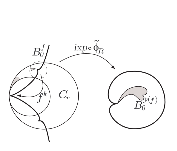
Figure 7. The formation of a “tail” in the immediate parabolic basin of ${\cal P}(f)$.

4.3. Definition of ${{{{\mathbf{P}}}}_{1}}$ and puzzle partitions

Definition 4.3.

We let ${{{{\mathbf{P}}}}_{1}}$ to be the collection of maps $f\in{{{{\mathbf{P}}}}}$ for which the point $t^{f}$ is accessible from the complement of the domain ${\cal D}(f)$. We thus have

$${{{{\mathbf{P}}}}_{0}}\subset{{{{\mathbf{P}}}}_{1}}\subset{{{{\mathbf{P}}}}}.$$

Theorem 4.6 will follow from a stronger statement:

Theorem 4.9.

Let $f\in{{{{\mathbf{P}}}}_{1}}$, and denote $B^{0}_{f}$ the immediate basin of the parabolic point $0$ of $f$. Then $B_{f}^{0}$ is a Jordan domain. Denote $\hat{f}$ the continuous extension of $f$ to $\partial B_{0}^{f}$. There exists a homeomorphism $\rho:\partial B_{0}^{f}\to{\mathbb{T}}$ such that

$$\rho(\hat{f}(z))=2\rho(z)\operatorname{mod}1.$$

Let us make a new definition. Let $f\in{{{{\mathbf{P}}}}_{1}}$. Consider an attracting petal $P_{A}^{f}$ which contains the unique critical value $c^{f}\in B_{0}^{f}$. Let $\tau\subset B_{0}^{f}$ be a simple curve which connects $c^{f}$ with the parabolic point $0$ and has the property $f(\tau)\subset\tau$. To fix the ideas, we will take this curve to be the horizontal ray

$$\{\operatorname{Re}(z)\geq\operatorname{Re}(\phi_{A}^{f}(c^{f})),\;\operatorname{Im}(z)=\operatorname{Im}(\phi_{A}^{f}(c^{f}))\}$$

in the Fatou coordinate. Using Proposition 4.8, and passing from a curve around the critical value to a slit connecting the critical value with a parabolic point we see:

Proposition 4.10.

There exists a unique simple curve $\Gamma^{\text{in}}$ connecting $t^{f}$ with $0$ such that

$$f(\Gamma^{\text{in}})=\tau.$$

By definition of ${{{{\mathbf{P}}}}_{1}}$, the tip of the tail $t^{f}\in\partial{\cal D}(f)$ is accessible from outside ${{\cal D}(f)}$. Let us continue $\Gamma^{\text{in}}$ by attaching a simple curve $\Gamma^{\text{out}}$ connecting $t^{f}$ to $\infty$ without intersecting $\overline{{\cal D}(f)}$. Let us further require that $\Gamma^{\text{out}}$ coincides with a negative real ray in a neighborhood of $\infty$.

Definition 4.4.

We call $\Gamma\equiv\overline{\Gamma^{\text{in}}\cup\Gamma^{\text{out}}}$ the primary cut of $f$.

We prove the following:

Proposition 4.11.

Let $f\in{{{{\mathbf{P}}}}_{1}}$. There exists a domain $U\subset{\mathbb{C}}$ such that:

• $U$ is a Jordan domain;

• $U\subset\operatorname{Dom}(f)$ and $\partial U\cup\partial\operatorname{Dom}(f)=\{t^{f}\}$;

• $\partial U\subset f^{-1}(\overline{\Gamma^{\text{out}}}\cup\partial\operatorname{Dom}(f))$ and $U\supset\Gamma^{\text{in}}$;

• $U\ni c^{f}$;

• there is a single critical point $p^{f}\in\Gamma^{\text{in}}$ of $f$ inside $U$.

Finally, there is a simple arc $\Gamma^{\text{in}}_{-1}\subset f^{-1}(\Gamma^{\text{in}})\cap U$ with endpoints $u^{+},u^{-}\in\partial U$ such that $\Gamma^{\text{in}}_{-1}\cap\Gamma^{\text{in}}=\{p^{f}\}$ for which the following holds:

• consider the Jordan domain $U^{\prime}$ which is the connected component of $U\setminus\Gamma^{\text{in}}_{-1}$ whose boundary does not contain the point $t^{f}$. Then

  $$f:U^{\prime}\setminus\Gamma^{\text{in}}\longrightarrow\operatorname{Dom}(f)\setminus\Gamma^{\text{in}}$$

  is a univalent map.

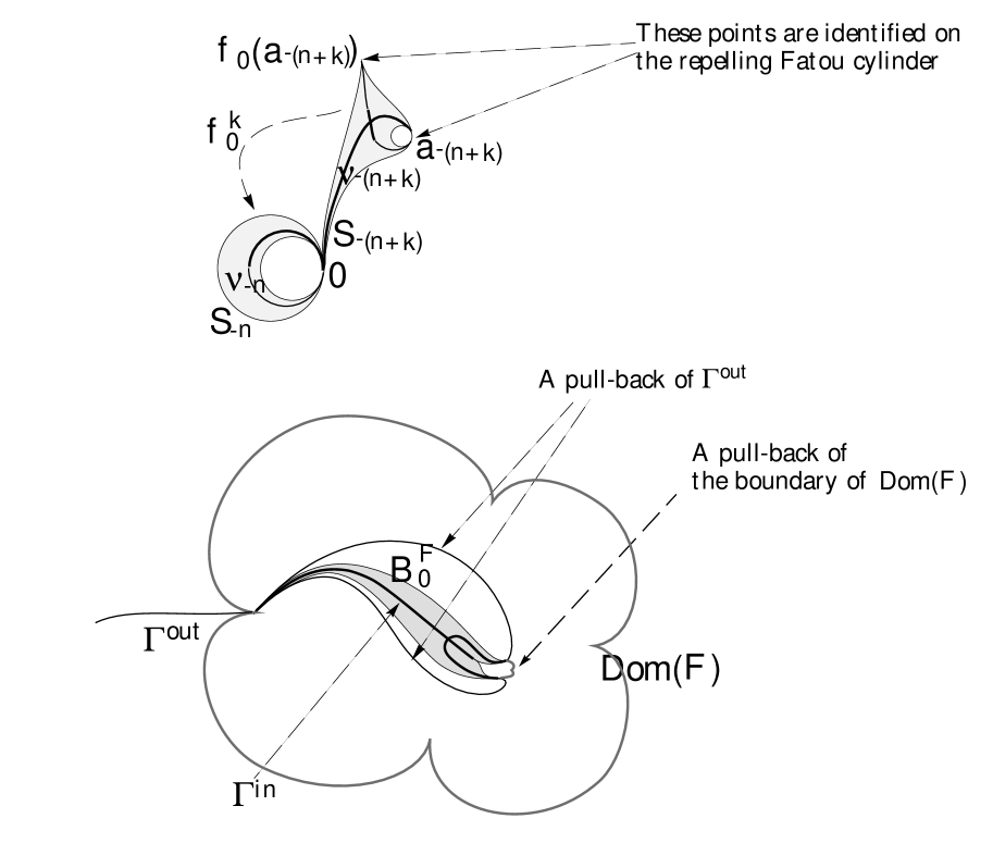
Figure 8. An illustration to the proof of Proposition 4.12. The pull-back of $\hat{\mathbb{C}}\setminus\Gamma$ for $F={\cal P}(f_{0})$.

In view of the definition of ${{{{\mathbf{P}}}}_{1}}$, it suffices to prove a slightly more general statement for $f=F\equiv{\cal P}(f_{0})$:

Proposition 4.12.

Let $F={\cal P}(f_{0})$. Consider any simple arc $\gamma=\gamma_{1}\cup\gamma_{2}$ and any Jordan curve $\tau$ with the following properties:

• $\gamma_{1}$ is a simple arc which connects $0$ and $t^{F}$;

• $\gamma_{2}$ is a simple arc which connects $t^{F}$;

• the curve $\gamma_{1}$ approaches $0$ within a sector $\{\operatorname{Arg}(z)\in(\pi/2,3\pi/2)\}$;

• the curve $\gamma_{2}$ approaches $\infty$ within a sector $\{\operatorname{Arg}(1/z)\in(\pi/2,3\pi/2)\}$;

• the curve $\tau$ separates $c^{F}$ from $\infty$ and $\tau\cap\gamma=\{t^{F}\}.$

There exists a domain $U$ of $F^{-1}(V)$ such that:

1. $U$ is a Jordan domain;

2. $U\subset\operatorname{Dom}(F)$ and $\partial U\cup\partial\operatorname{Dom}(F)=t^{F}$;

3. $\partial U\subset F^{-1}(\overline{\gamma_{2}}\cup\tau);$

4. $U$ contains a single critical point $p^{F}$;

5. there is a simple arc $\delta\subset U$ which is a preimage of $\gamma_{1}$, has endpoints on the boundary of $U$, and intersects $\gamma_{1}$ at the critical point $p^{F}$ only. If we let $U^{\prime}$ be the component of $U\setminus\delta$ not containing $t^{F}$ on the boundary, then the map

   $$F:U^{\prime}\longrightarrow\operatorname{Dom}(F)\setminus F(\delta)$$

   is univalent.

Proof.

Let us again begin by selecting a simple curve $\sigma\subset\hat{\mathbb{C}}$ which connects $0$ and $\infty$, and does not intersect with $\gamma\cup\tau$ except at the point $0$, and such that an analytic branch of the logarithm defined on a neighborhood of $\sigma$ has bounded imaginary part.

Let us parametrize $\gamma$:

$$\gamma(t):[0,1]\to\hat{\mathbb{C}}$$

so that $\gamma(0)=0$ and $\gamma(1)=\infty$.

With a slight abuse of notation we use the same notation for the preimages of $\sigma$ and $\gamma$, etc. as in the proof of Proposition 4.8. Let $S_{-n}$ be the fundamental crescent $P_{-n}\setminus\overline{f(P_{-n})}$ which contains the critical value $-1/4$. The corresponding component $\nu_{-n}\subset\overline{S_{-n}}$ of the lift of $\gamma$ is a simple arc which passes through $-1/4$, and whose two ends land at $0$.

There are two prime ends of the point $0$ in the crescent $S_{-n}$. We denote the “upper” one by $0_{-n}^{+}$, and the “lower” one by $0_{-n}^{-}$. They correspond to the points $0$ and $\infty$ respectively in the quotient ${\cal C}_{A}\simeq\hat{\mathbb{C}}$. We will write

$$\nu_{-n}(t)\underset{t\to 0+}{\longrightarrow}0^{+}_{-n}\text{ and }\nu_{-n}(t)\underset{t\to 1-}{\longrightarrow}0^{-}_{-n}.$$

Writing $S_{-(n+k)}=P_{-(n+k)}\setminus P_{-(n+k-1)}$, we see that

$$f_{0}:S_{-(n+1)}\to S_{-n}$$

is a double covering, branched at

$$-1/2\mapsto-1/4\in\nu_{-n}.$$

We thus obtain two parametrized curves $\nu^{1}_{-(n+1)}$ and $\nu^{2}_{-(n+1)}$ as the lifts of $\nu_{-n}$ by $f_{0}$. The intersection

$$\overset{\circ}{\nu}^{1}_{-(n+1)}\cap\overset{\circ}{\nu}^{2}_{-(n+1)}=-1/2.$$

For $j\leq n+1$ we denote $0_{-j}^{+}$, $0_{-j}^{-}$ the “upper” and the “lower” prime ends of $0$ in $S_{-j}$, so that

$$\tilde{f}_{0}:0^{\pm}_{-j}\mapsto 0^{\pm}_{-(j-1)}.$$

The other preimage of $0$ in $\partial S_{-(n+1)}$ is the point $-1$. We use $-1_{-(n+1)}^{+}$ and $-1_{-(n+1)}^{-}$ to denote its two prime ends in $S_{-(n+1)}$ labeled so that the Carathéodory extension $\tilde{f}_{0}$ maps

$$-1_{-(n+1)}^{+}\mapsto 0^{+}_{-n}\text{ and }-1_{-(n+1)}^{-}\mapsto 0^{-}_{-n}.$$

We have

$$\nu^{1}_{-(n+1)}(t)\underset{t\to 0+}{\longrightarrow}0^{+}_{-(n+1)}\text{ and }\nu_{-(n+1)}(t)\underset{t\to 1-}{\longrightarrow}-1^{-}_{-(n+1)};$$

$$\nu^{2}_{-(n+1)}(t)\underset{t\to 0+}{\longrightarrow}-1^{+}_{-(n+1)}\text{ and }\nu_{-(n+1)}(t)\underset{t\to 1-}{\longrightarrow}0^{-}_{-(n+1)}.$$

Denote $S_{-(n+k)}\subset W$ the pull-back of $S_{-(n+k-1)}$ by the inverse branch ${g_{0}}$; and

$$\nu^{1,2}_{-(n+k)}\subset S_{-(n+k)}$$

the corresponding preimage of $\nu_{-n}$. A trivial induction shows that there are exactly three points

$$\{0,a_{-(n+k)},f(a_{-(n+k)})\}\subset\partial S_{-(n+k)},$$

which map to $0$ under $f_{0}^{k}$. Furthermore, $a_{-(n+k)}$ has two prime ends in $S_{-(n+k)}$; the points $0$ and $f_{0}(a_{-(n+k)})$ each have a single prime end. We denote $a_{-(n+k)}^{\pm}$ the prime end mapped to $0_{-n}^{\pm}$ by the Carathéodory extension $\tilde{f}_{0}^{k}$.

We have

$$\nu^{1}_{-(n+k)}(t)\underset{t\to 0+}{\longrightarrow}0_{-(n+k)}\text{ and }\nu_{-(n+1)}(t)\underset{t\to 1-}{\longrightarrow}f_{0}(a_{-(n-k)});$$

$$\nu^{2}_{-(n+k)}(t)\underset{t\to 0+}{\longrightarrow}a^{+}_{-(n+1)}\text{ and }\nu_{-(n+k)}(t)\underset{t\to 1-}{\longrightarrow}a^{-}_{-(n+1)}.$$

Each of the sets $\nu_{-j}$ is composed of two parts, $\nu_{-j,1}$ and $\nu_{-j,2}$ which are the preimages of $\gamma_{1}$ and $\gamma_{2}$ respectively. For $j\leq n$, they intersect at a single point $b_{-j}$; for $j>n$ there are two such points $b^{1}_{-j}$, $b^{2}_{-j}$.

Denote $\kappa_{-(n+k)}\subset S_{-(n+k)}$ the preimage of $\tau$. Elementary considerations of monodromy, which we spare the reader, imply that $\kappa_{-(n+k)}$ is a union of two simple arcs: one connecting $0$ with $b^{1}_{-(n+k)}$, the other with $b^{2}_{-(n+k)}$; and otherwise disjoint from $\nu_{-(n+k)}$.

Considerations of Denjoy-Wolff Theorem imply that for every ample repelling petal $P_{R}$ there exists $k$ such that $S_{-(n+k)}\subset P_{R}$. Let us project the picture in $S_{-(n+k)}$ back to $\hat{\mathbb{C}}$ using $\operatorname{ixp}\circ\phi_{R}^{f_{0}}$. The points $a_{-(n+k)}$ and $f_{0}(a_{-(n+k)})$ are identified in the projection. We obtain a Jordan domain $U$, bounded by the projections of $\kappa^{1}_{-(n+k)}$, $\kappa^{2}_{-(n+k)}$, $\nu_{-(n+k),2}$. It satisfies the properties (1)-(5) by the construction.

∎

Corollary 4.13.

Let $f\in{{{{\mathbf{P}}}}_{1}}$, and let $U$ be the domain constructed in Proposition 4.11. We have

• $B_{0}^{f}\subset U$;

• $\partial B_{0}^{f}\cap\partial\operatorname{Dom}(f)=\{t^{f}\}$.

Proof.

Since $B_{0}^{f}$ does not intersect with $\overline{\Gamma^{\text{out}}}\cup\partial\operatorname{Dom}(f)$ and $\partial U\subset f^{-1}(\overline{\Gamma^{\text{out}}}\cup\partial\operatorname{Dom}(f))$, we have $B_{0}^{f}\subset U$. Hence,

$$\partial B_{0}^{f}\cap\partial\operatorname{Dom}(f)\subset\{t^{f}\}.$$

On the other hand, the cut $\Gamma^{\text{in}}\subset B_{0}^{f}$, hence

$$t^{f}\in\overline{\Gamma^{\text{in}}}\in\partial B_{0}^{f}.$$

∎

4.4. The immediate basin of a map in ${{{{\mathbf{P}}}}_{1}}$ is a Jordan domain

We are now in a position to begin the proof of Theorem 4.9, which in turn implies Theorem 4.6. Let us fix $F\in{{{{\mathbf{P}}}}_{1}}$ and let $U$ be the domain constructed in Proposition 4.11. The preimage $\overline{F^{-1}(\Gamma^{\text{in}})}\cap B_{0}^{F}$ consists of the curve $\Gamma^{\text{in}}$ and a simple curve $\Gamma^{\text{in}}_{-1}$; the two curves cross at the critical point $p^{F}\in B_{0}^{F}$. To fix the ideas, let us parametrize

$$\Gamma^{\text{in}}:[0,1]\to\overline{B}_{0}^{f}$$

so that $\Gamma^{\text{in}}(0)=0$ and $\Gamma^{\text{in}}(1)=t^{f}$. Let $s_{1}<s_{2}\in(0,1)$ be such that

$$\Gamma^{\text{in}}(s_{1})=c^{F},\;\Gamma^{\text{in}}(s_{2})=p^{F}.$$

By elementary path-lifting considerations, the curve $\Gamma^{\text{in}}_{-1}$ is a cross-cut in $U$. Let $V$ be the connected component of $U\setminus\Gamma^{\text{in}}_{-1}$ which does not contain $t^{F}$ in its boundary. By construction (Proposition 4.11), there exists a univalent branch $G$ of $F^{-1}$ which maps

$$\operatorname{Dom}(F)\setminus\Gamma^{\text{in}}([s_{1},1])\mapsto V\setminus\Gamma^{\text{in}}([s_{1},s_{2}]).$$

We note:

Proposition 4.14.

The inverse branch $G$ maps the domain $\operatorname{Dom}(F)\setminus\Gamma^{\text{in}}$ inside itself.

Let $l(t)$ be a simple path such that $l(0)=u$, $l(1)=F(u)\in\partial\operatorname{Dom}(F)$, and $\overset{\circ}{l}\cap\overline{U}=\emptyset.$ Since $\operatorname{Dom}(F)$ is a Jordan domain, the inverse branch $G$ has a continuous extension to the boundary point $u$. Set $u_{0}\equiv u$, and denote $u_{-n}$ the orbit of $u_{0}$ under $G$. The curve $l$ has a univalent pull-back $l_{-1}\subset\overline{V}$ such that $l_{-1}(0)=u_{-1}$ and $l_{-1}(1)=u.$ We let

$$l_{-n}=G(l_{-(n-1)})\text{ for }n\geq 2.$$

Set

$$\Lambda=\cup_{n\geq 1}l_{-n}.$$

We parametrize this curve by $(0,1]$ so that

$$\Lambda\left(\left[\frac{1}{j},\frac{1}{j-1}\right]\right)=l_{-(j-1)}\text{ for }j\geq 2.$$

Thus, $\Lambda(1/j)=u_{-j}.$ By Proposition 4.14 and Denjoy-Wolff Theorem, we have:

Proposition 4.15.

The curve $\Lambda$ is disjoint from $B_{0}^{F}$, and lands at $0$:

$$\lim_{t\to 0-}\Lambda(t)=0.$$

Definition 4.5.

We call the curve $\hat{\Gamma}\equiv\Gamma\cup\Lambda$ the secondary cut.

Let $u^{+},u^{-}\in\partial U$ be the two endpoints of $\Gamma^{\text{in}}_{-1}$, labeled in such a way that $u^{+}$ is encountered first, when going around $\partial U$ in the positive direction from $t^{f}$. Denote the connected components of $U\setminus\hat{\Gamma}$ by $U^{+}$, $U^{-}$ so that $U^{\pm}\ni u^{\pm}$.

Consider the inverse branch of $f$ which maps $B_{0}^{F}\setminus\Gamma^{\text{in}}([0,s_{1}])$ into $B_{0}^{F}\cap U^{+}$, and let $G_{0}$ be its univalent extension to

$$G_{0}:U\setminus(\Lambda\cup\Gamma^{\text{in}}([0,s_{1}]))\hookrightarrow U^{+}.$$

Replacing $U^{+}$ with $U^{-}$ we similarly define an analytic branch of $F^{-1}$

$$G_{1}:U\setminus(\Lambda\cup\Gamma^{\text{in}}([0,s_{1}]))\hookrightarrow U^{-}.$$

Let $P\subset B_{0}^{F}$ be an attracting petal which contains $c^{F}$ in its interior, and let $P_{-1}$ be a connected component of $F^{-1}(P)$ such that

$$P\subset P_{-1}.$$

We set

$${\mathbf{A}}\equiv U\setminus P_{-1}.$$

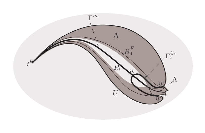
Figure 9. The domain ${\mathbf{A}}$.

Let

$${\mathbf{A}}_{0}\equiv{\mathbf{A}}\cap U^{+}\quad\text{and}\quad{\mathbf{A}}_{1}\equiv{\mathbf{A}}\cap U^{-}$$

If $i_{0}i_{1}\ldots i_{n}$ is an arbitrary sequence of $n+1$ 0’s and 1’s, we define

$${\mathbf{A}}_{i_{0}i_{1}\ldots i_{n}}:=\{z\in{\mathbf{A}}_{0}:f^{j}(z)\in{\mathbf{A}}_{i_{j}}\quad\text{for}\quad 1\leq j\leq n\}$$

The proof of Theorem 4.9 now follows the same lines as in §3.3. It follows from the definitions that

• ${\mathbf{A}}_{i_{0}i_{1}\ldots i_{n}}$ is decreasing in $n$: ${\mathbf{A}}_{i_{0}\ldots i_{n}}\subset{\mathbf{A}}_{i_{0}\ldots i_{n-1}};$

• $F{\mathbf{A}}_{i_{0}i_{1}\ldots i_{n}}={\mathbf{A}}_{i_{1}\ldots i_{n}};$

• ${\mathbf{A}}_{i_{0}i_{1}\ldots i_{n}}={G_{i_{0}}}{\mathbf{A}}_{i_{1}\ldots i_{n}},$ and hence

  $${\mathbf{A}}_{i_{0}i_{1}\ldots i_{n}}={G_{i_{0}}}\circ{G_{i_{1}}}\circ\cdots\circ{G_{i_{n-1}}}{\mathbf{A}}_{i_{n}},$$

  or, more generally,

  $${\mathbf{A}}_{i_{0}i_{1}\ldots i_{n}}={G_{i_{0}}}\circ{G_{i_{1}}}\circ\cdots\circ{G_{i_{j-1}}}{\mathbf{A}}_{i_{j}i_{j+1}\ldots i_{n}}\quad\text{for $1\leq j\leq n-1$.}$$

We show that the diameters of the puzzle pieces ${\mathbf{A}}_{i_{0}i_{1}\ldots i_{n}}$ go to zero as $n\to\infty$, uniformly in $i_{0}i_{1}\ldots i_{n}$. More precisely, let us define

$$\rho_{n}:=\sup\left\{\text{diam}({\mathbf{A}}_{i_{0}\ldots i_{n}}):i_{0}\ldots i_{n}\in\{0,1\}^{n+1}\right\}$$

Since ${\mathbf{A}}_{i_{0}\ldots i_{n}}\supset{\mathbf{A}}_{i_{0}\ldots i_{n+1}}$, the sequence $\rho_{n}$ is non-increasing in $n$, so

(4.1) $$\rho_{*}:=\lim_{n\to\infty}\rho_{n}$$

exists.

We will prove

Proposition 4.16.

The limit $\rho_{*}=0.$

In the same way as Lemma 3.16, we have

Lemma 4.17.

There is an infinite sequence $i_{0}i_{1}\ldots i_{n}\ldots$ so that

$$\operatorname{diam}(A_{i_{0}i_{1}\ldots i_{n}})\geq\rho_{*}\quad\text{for all $n$.}$$

Proof of Proposition 4.16.

Let us assume the contrary: $\rho_{*}>0$.

We fix a sequence $i_{0}i_{1}\ldots$ as in the Lemma 3.16, and we split the proof into three cases:

1. $i_{j}$ is eventually 0;

2. $i_{j}$ is eventually 1;

3. neither of the above holds.

We start with case (3). There are then infinitely many $j$’s so that

$$i_{j}=0\quad\text{and}\quad i_{j+1}=1$$

Let $j_{k}$ be a strictly increasing sequence of such $j$’s. Then, for each $k$,

$$f_{-j_{k}}:={G_{i_{0}}}\circ{G_{i_{1}}}\circ\cdots\circ{G_{i_{j_{k}-1}}}$$

is an analytic branch of the inverse of $f_{0}^{j_{k}}$ mapping ${\mathbf{A}}_{01}$ bijectively to ${\mathbf{A}}_{i_{0}\ldots i_{j_{k}+1}}$. The closure of ${\mathbf{A}}_{01}$ does not intersect the postcritical set of $f$. We now use a version of the argument we gave the proof of Theorem 3.15.

We let $Q$ be an simply connected open neighborhood of $\overline{{\mathbf{A}}_{01}}$ disjoint from the postcritical set. Then each $f_{-j_{k}}$ extends to an analytic branch of the inverse of $F^{j_{k}}$ defined on $Q$ (and we denote this extension also by $f_{-j_{k}}$).

By Montel’s Theorem, there is a subsequence of $(j_{k})$ along which $f_{-j_{k}}$ converges uniformly on compact subsets of $U$ in the spherical metric on $\hat{\mathbb{C}}$. By adjusting the notation, we can assume that the sequence $(f_{-j_{k}})$ itself converges to an analytic function which we denote $h$. Since

$$\text{diam}(f_{-j_{k}}{\mathbf{A}}_{01})=\text{diam}({\mathbf{A}}_{i_{0}\ldots i_{j_{k}+1}})$$

does not go to zero as $k\to\infty$, the function $h$ is non-constant.

Let $z_{0}:={G_{0}}(u^{-})\in{\mathbf{A}}_{01}\cap\partial B_{0}^{f}$. By invarince of the basin boundary, we have $w_{0}=h(z_{0})\in\partial B_{0}^{f}$. Since $h$ is non-constant, $h({\mathbf{A}}_{01})$ contains an open neighborhood $W$ of $w_{0}$. Let $V\Subset W$ be a smaller open neighborhood of $w_{0}$. Then, an arbitrary large iterate $F^{j_{k}}$ maps $V$ inside $Q$, which is impossible, since $f(u^{-})=t^{f}\in\partial\operatorname{Dom}(f)$.

We turn next to case 1 above, and deal first with the situation $i_{j}=0$ for all $j$. We write

$${\mathbf{A}}^{(n)}:={\mathbf{A}}_{\underbrace{0\cdots 0}_{\text{$n$ terms}}}=({G_{0}})^{n-2}{\mathbf{A}}_{00}$$

Now ${G_{0}}$ maps ${\mathbf{A}}_{00}$ into itself, and ${G_{0}}={G}$ on ${\mathbf{A}}_{00}$, so we can write

$${\mathbf{A}}^{(n)}=({G})^{n-2}{\mathbf{A}}_{00}.$$

By Denjoy-Wolff Theorem applied to $g$ and local dynamics near the parabolic point $0$,

$$({G})^{n-2}\to 0\quad\text{uniformly on ${\mathbf{A}}_{00}$},$$

so

$$\text{diam}({\mathbf{A}}^{(n)})\to 0\quad\text{as $n\to\infty$.}$$

Next consider sequences of the form $i_{0}i_{1}\cdots i_{k}00\cdots$, and use the formula

$${\mathbf{A}}_{i_{0}\ldots i_{k}\underbrace{0\cdots 0}_{\text{$n$ terms}}}={G_{i_{0}}}\circ{G_{i_{1}}}\circ\cdots\circ{G_{i_{k}}}A^{(n)}.$$

The mapping ${G_{i_{0}}}\circ{G_{i_{1}}}\circ\cdots\circ{G_{i_{k}}}$ extends to be continuous on $\overline{{\mathbf{A}}_{00}}$, and $\text{diam}(A^{(n)})\to 0$ by what we just proved, so

$$\text{diam}({\mathbf{A}}_{i_{0}\ldots i_{k}\underbrace{0\cdots 0}_{\text{$n$ terms}}})\to 0\quad\text{as $n\to\infty$.}$$

A similar argument, using ${G_{1}}={G}$ on ${\mathbf{A}}_{11}$ shows that

$$\text{diam}({\mathbf{A}}_{i_{0}\ldots i_{k}\underbrace{1\cdots 1}_{\text{$n$ terms}}})\to 0\quad\text{as $n\to\infty$.}$$

∎

Let ${\mathbf{i}}=(i_{j})_{j=0}^{N}$ be a finite or infinite sequence ($N\leq\infty$) of $0$’s and $1$’s. We interpret it as a binary representation of a number in $[0,1]$:

$${\underline{\mathbf{i}}}_{2}\equiv\sum_{j=0}^{N}i_{j}2^{j}\in[0,1].$$

For any such dyadic sequence,

$$\overline{{\mathbf{A}}_{i_{0}}}\supset\overline{{\mathbf{A}}_{i_{0}i_{1}}}\supset\cdots\supset\overline{{\mathbf{A}}_{i_{0}\ldots i_{n}}}\supset\ldots$$

is a nested sequence of compact sets in ${\mathbb{C}}$ with diameter going to 0, so its intersection contains exactly one point, which we denote by $\hat{z}({\mathbf{i}})$. It is immediate from the construction that ${\mathbf{i}}\mapsto\hat{z}({\mathbf{i}})$ is continuous from $\{0,1\}^{\mathbb{Z}}$ to ${\mathbb{C}}$. It is not injective, however, this ambiguity is easily tractable:

Lemma 4.18.

Suppose ${\mathbf{i}}=i_{0}i_{1}\ldots i_{n-1}$ and ${\mathbf{i}}^{\prime}=i^{\prime}_{0}i^{\prime}_{1}\ldots i^{\prime}_{n-1}$ are two finite dyadic sequences of an equal length, and

$$\overline{{\mathbf{A}}_{{\mathbf{i}}}}\cap\overline{{\mathbf{A}}_{{\mathbf{i}}^{\prime}}}\neq\emptyset.$$

Then either ${\underline{\mathbf{i}}}_{2}={\underline{\mathbf{i}^{\prime}}}_{2},$ or ${\underline{\mathbf{i}}}_{2}={\underline{\mathbf{i}^{\prime}}}_{2}\pm 2^{-n}.$

The proof is a straightforward induction in $n$, and is left to the reader.

As a corollary, we get:

Corollary 4.19.

Let ${\mathbf{i}}$ and ${\mathbf{i}^{\prime}}$ be two infinite dyadic sequences. If ${\underline{\mathbf{i}}}_{2}\neq{\underline{\mathbf{i}^{\prime}}}_{2}$, then $\overline{{\mathbf{A}}_{i_{0}\cdots i_{n}}}$ and $\overline{{\mathbf{A}}_{i^{\prime}_{0}\cdots i^{\prime}_{n}}}$ are disjoint for large enough $n$

Proof.

For any ${\mathbf{i}}=i_{0}\cdots i_{n}\cdots$, and any $n$

$$|{\underline{\mathbf{i}}}_{2}-\underline{i_{0}\cdots i_{n-1}}_{2}|\leq 2^{-n}$$

so, if $n$ is large enough so that

$$|{\underline{\mathbf{i}}}_{2}-{\underline{\mathbf{i}^{\prime}}}_{2}|>3\times 2^{-n},$$

then

$$|\underline{i_{0}\cdots i_{n-1}}_{2}-\underline{i^{\prime}_{0}\cdots i^{\prime}_{n-1}}_{2}|>2^{-n},$$

which by Lemma 3.17 implies that $\overline{{\mathbf{A}}_{i_{0}\cdots i_{n-1}}}$ and $\overline{{\mathbf{A}}_{i^{\prime}_{0}\cdots i^{\prime}_{n-1}}}$ are disjoint, as asserted. ∎

Putting together what we know about the map ${\mathbf{i}}\mapsto\hat{z}({\mathbf{i}})$, we finally obtain:

Proposition 4.20.

The angles ${\underline{\mathbf{i}}}_{2}={\underline{\mathbf{i}^{\prime}}}_{2}$ if and only if $\hat{z}({\mathbf{i}})=\hat{z}({\mathbf{i}^{\prime}})$. Hence there is a function $\theta\mapsto z(\theta)$ from the circle ${\mathbb{R}}/{\mathbb{Z}}$ to ${\mathbb{C}}$ so that

$$\hat{z}({\mathbf{i}})={\underline{\mathbf{i}}}_{2}.$$

The function $z(\,.\,)$ is continuous, bijective, and maps the circle onto

$$J\equiv\overline{\cap_{n}((F^{-n})|_{U}\overline{{\mathbf{A}}})}.$$

We thus have:

Corollary 4.21.

The set $J$ is a Jordan curve.

Proposition 4.22.

Let $\tilde{F}:J\to J$ be defined as $\tilde{F}(t^{F})=0$, and coincide with $F$ elsewhere on $J$. The map ${\underline{\mathbf{i}}}_{2}\mapsto\hat{z}({\mathbf{i}})$ is a conjugacy between $\theta\mapsto 2\theta$ and $\tilde{F}(z)$:

$$\tilde{F}(\hat{z}({\mathbf{i}}))=\hat{z}(2\cdot{\underline{\mathbf{i}}}_{2}).$$

Let us denote $B$ the connected component of $\hat{\mathbb{C}}\setminus J$ which contains $c^{F}$. By construction, $B\cap B_{0}^{F}\neq\emptyset$. By the Maximum Principle,

$$F:B\to B.$$

By the classification of dynamics on a hyperbolic domain,

$$B\subset B_{0}^{F}.$$

On the other hand, preimages of $t^{f}$ are dense in $J=\partial B$, and hence

$$B_{0}^{F}\cap J=\emptyset.$$

We conclude:

$$B=B_{0}^{F},$$

and thus Theorem 4.9 is proven.

We illustrate the topological structure of the parabolic basin of a map $f\in{\cal P}({{{{\mathbf{P}}}}_{0}})$ in Figure 10. We have indicated the immediate basin $B_{0}$ as well as several components of $f^{-1}(B_{0})$. To better understand those, we have drawn the preimage $f^{-1}(C)$ of the circle

$$C=\{|z|=|c|\},$$

which cuts across the only critical value $c$ of $f$. These critical level curves partition the domain $W$ into univalent preimages of the disks $D^{+}=D_{|c|}(0)$ and $D^{-}=\hat{\mathbb{C}}\setminus\overline{D^{+}}$.

Two smooth branches in the preimage $f^{-1}(C)$ may intersect at a ramification point of $f$ (all of the ramification points are simple). Each critical component of $f^{-1}(B_{0})$ has one of these branch points, and touches $\partial W$ in two points (“preimages” of the asymptotic value $0$). The non-critical components of $f^{-1}(B_{0})$ arrange themselves in sequences along the critical level curves, as shown.

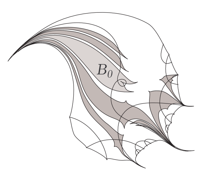
Figure 10. Several components of the parabolic basin of $f\in{{{{\mathbf{P}}}}_{0}}$

4.5. Convergence of parabolic renormalization

By definition of the class ${{{{\mathbf{P}}}}_{0}}$, every map $f\in{{{{\mathbf{P}}}}_{0}}$ can be decomposed as

$$f=v\cdot{\cal P}(f_{0})\circ\varphi_{f}(e^{2\pi i\theta}z):\operatorname{Dom}(f)\to\hat{\mathbb{C}},$$

where $v=c^{f}/c^{{\cal P}(f_{0})}.$ We will denote $\psi_{f}=\varphi_{f}^{-1}$. Thus, $\varphi_{f}$ conformally maps the unit disk ${\mathbb{D}}$ onto $W_{f}=\text{Dom}(f)$ with $\psi_{f}(0)=0$ and $\psi_{f}^{\prime}(0)>0$. We will topologize ${{{{\mathbf{P}}}}_{0}}$ by identifying it with the space of thus normalized conformal maps of the unit disk:

$$f\mapsto\psi_{f},$$

equipped with the compact-open topology.

Let us state an obvious consequence of the Koebe Distortion Theorem:

Lemma 4.23.

Let ${\cal S}$ be a family of univalent maps $h:{\mathbb{D}}\to\hat{\mathbb{C}}$ with $h(0)=0$. Assume further that there exist positive constants $0<a<b$ such that $a\leq|h^{\prime}(0)|\leq b$ for every $h\in{\cal S}$. Then the family ${\cal S}$ is equicontinuous.

H. Inou and M. Shishikura [IS] have recently demonstrated the following:

Theorem 4.24 ([IS]).

There exists a class $\mathbf{F}$ of analytic maps with a simple parabolic fixed point at the origin, such that the following properties hold:

• ${\cal P}({\mathbf{F}})\subset({\mathbf{F}})$;

• there exists a map $f_{*}\in\mathbf{F}$ which is a fixed point of the parabolic renormalization:

  $${\cal P}(f_{*})=f_{*};$$

• denoting $f_{0}(z)=z+z^{2}$, we have ${\cal P}(f_{0})\in\mathbf{F}$, and

  $${\cal P}^{n}(f_{0})\to f_{*}\text{ in }\mathbf{F};$$

• in fact, there is a structure of an infinite-dimensional complex-analytic manifold on $\mathbf{F}$ which is compatible with the local-uniform norm, in which ${\cal P}$ is a contraction.

We remark:

Corollary 4.25.

The fixed point $f_{*}$ has an analytic extension to a mapping in ${{{{\mathbf{P}}}}_{0}}$ which we will denote in the same way. It is also fixed under ${\cal P}$, considered as a transformation ${{{{\mathbf{P}}}}_{0}}\to{{{{\mathbf{P}}}}_{0}}$.

Proof.

By Lemma 4.23, the sequence of parabolic renormalizations ${\cal P}^{n}(f_{0})$ is pre-compact in ${{{{\mathbf{P}}}}_{0}}$. By Theorem 4.24, every limit point of this sequence coincides with $f_{*}$ on a neighborhood of the origin. ∎

5. Numerical results

5.1. Properties of the asymptotic expansion of the Fatou coordinates

A justification of the use of the asymptotic expansion of the Fatou coordinate (Theorem 2.15) for computation has a theoretical basis in the following. Recall (see e.g. [Ram]) that a formal power series $\sum_{m=1}^{\infty}a_{m}x^{-m}$ is of Gevrey order $k$ if

$$|a_{m}|<CA^{n}(n!)^{\frac{1}{k}}\text{ for some choice of positive constants }C,A.$$

As was shown by Écalle [Ec]:

Theorem 5.1.

The asymptotic expansion of Theorem 2.15 is of Gevrey order $1$.

Thus, the asymptotic series of $g(w)$ is rather slowly divergent. A Stirling formula estimate suggest that the first $n$ terms of the series are useful in estimating the value of $g$ for $|w|>\text{const}\cdot n$.

Theorem 5.1 is a part of Écalle’s theory of resurgence as applied specifically to Fatou coordinates (see [Sau] for an account). Recall, that the Borel transform of a formal power series $\sum_{m=1}^{\infty}a_{m}x^{-m}$ consists in applying the termwise inverse Laplace transform:

$$a_{m}x^{-m}\mapsto\frac{a_{m}\zeta^{m-1}}{(m-1)!}.$$

In the case when the formal power series is of Gevrey order $1$, this yields a series

$$\sum_{m=1}^{\infty}\frac{a_{m}\zeta^{m-1}}{(m-1)!},$$

which converges to an analytic function $\hat{h}(\zeta)$ in a neighborhood of the origin. Assume further, that the function $\hat{h}$ extends analytically along the positive real axis, and the extension is of an exponential type. Then, the Laplace transform

$$h(x)=\int_{0}^{\infty}e^{-x\zeta}\hat{h}(\zeta)d\zeta$$

is defined when $\operatorname{Re}x$ is sufficiently large. The original formal power series $\sum_{m=1}^{\infty}a_{m}x^{-m}$ is the asymptotic series of $h(x)$, which should thus be considered a summation of the divergent formal series.

Resurgence theory implies much more detailed information about the asymptotic expansion of the Fatou coordinate given in Theorem 2.15, than that required to perform the Borel summation. In particular, the function $\hat{h}$ analytically extends not just along the positive real axis, but along every path in ${\mathbb{C}}\setminus\{2\pi in,\;n=\pm 1,\pm 2,\ldots\}.$ The attracting Fatou coordinate is obtained using the Laplace transform as described above. The same function $\hat{h}$ also produces the repelling Fatou coordinate: by using the Laplace transform

$$\int_{-\infty}^{0}e^{-x\zeta}\hat{h}(\zeta)d\zeta$$

for $x$ with a large negative real part. The development of the resurgence theory for Fatou coordinates was started by Écalle in [Ec], and was largely completed in the recent work of Dudko and Sauzin [DS].

5.2. Computational scheme for ${\cal P}$

Having mentioned the resurgent properties of the asymptotic expansion of the Fatou coordinate, we proceed to describe the computational scheme for ${\cal P}$. We begin with a germ of an analytic mapping

$$f(z)=z+z^{2}+O(z^{3})$$

defined in a neighborhood of the origin. Applying the change of coordinates $w=\kappa(z)=-1/z$, we obtain

$$F(w)=w+1+\frac{A}{w}+O\left(\frac{1}{w^{2}}\right)$$

defined in a neighborhood of $\infty$. We again use the notation $\Phi_{A}(w)$ for the function which conjugates $F$ with the unit translation

$$\Phi_{A}(F(w))=\Phi_{A}(w)+1$$

for $\operatorname{Re}w>>1$. We let $\Phi_{R}(w)$ be the solution of the same functional equation for $\operatorname{Re}w<<-1$. These changes of coordinate are well-defined up to an additive constant, and

$$\phi_{A}(z)=\kappa^{-1}\circ\Phi_{A}\circ\kappa(z),\;\phi_{R}(z)=\kappa^{-1}\circ\Phi_{R}\circ\kappa(z).$$

As we have seen in Theorem 2.15, the function $\Phi_{A}(w)$ has an asymptotic development

$$\Phi_{A}(w)\sim w-A\log w+\text{const}_{A}+\sum_{k=1}^{\infty}b_{k}w^{-k}.$$

The coordinate $\Phi_{R}(w)$ has an identical asymptotic development, differing only by the value of $\text{const}_{R}$. While this may seem surprising at first glance, recall that these functions are Laplace transforms of different analytic continuations of the Borel transform of the same divergent series (plus the $w-A\log w+\text{const}$ term).

We select a large integer $M$ (in practice, $M\approx 100$). We will use the asymptotic expansion to estimate $\Phi_{A}(w)$ for $w\geq M$ and $\Phi_{R}(w)$ for $w\leq-M$. Consider an iterate $N\approx 2M$ such that

$$\operatorname{Re}F^{N}(w)\geq M\text{ for }\operatorname{Re}w\in[-M-1,-M].$$

Denote $\nu(z)$ the function

$$\nu(z)=\operatorname{ixp}\circ\Phi_{A}\circ F^{N}\circ(\Phi_{R})^{-1}\circ\operatorname{ixp}^{-1}(z).$$

It differs from the parabolic renormalization ${\cal P}(f)$ only by rescaling the function and its argument:

$${\cal P}(f)(z)=a_{1}\nu(a_{0}z).$$

Now consider a contour $\Gamma$ connecting $w=-M-1+iH$ with $F(w)\approx-M+iH$ which is mapped onto the circle $S_{\rho}=\{|z|=\rho\}$ for a small value of $\rho$ by $\operatorname{ixp}\circ\Phi_{R}$. Select $n\in{\mathbb{N}}$ and consider the $n$ points in $S_{\rho}$ given by $x_{k}=\rho\exp(2\pi k/n),\;k=0,\ldots,n-1$. We then evaluate the first $n$ coefficients in the Taylor expansion of $\eta$ at the origin

$$\eta(z)=\sum_{j=0}^{\infty}r_{j}z^{j}$$

using a discrete Fourier transform. Specifically, we calculate

$$s_{k}=\nu(x_{k})\approx\sum_{j=0}^{n-1}r_{j}(x_{k})^{j}=\sum_{j=0}^{n-1}r_{j}\rho^{j}\exp(2\pi kj/n),$$

and apply the inverse discrete Fourier transform:

$$r_{j}\approx\frac{1}{n\rho^{j}}\sum_{k=0}^{n-1}s_{k}\exp(-2\pi kj/n).$$

Since

$${\cal P}(f)(z)=\sum_{j=1}^{\infty}s_{j}a_{1}a_{0}^{j}z^{j},$$

we have

$$a_{1}a_{0}s_{1}=1,\text{ and further }a_{0}=\frac{s_{1}}{s_{2}}.$$

This step completes the computation of the Taylor expansion of ${\cal P}(f)$.

5.3. Computing $f_{*}$

In computing the fixed point $f_{*}(z)$ we find it more convenient to work with the representation of a germ $f(z)=z+z^{2}+\cdots$ in the form:

$$f(z)=z\exp(f_{\log}(z)),$$

where $f_{\log}$ is a germ of an analytic function at the origin with $f_{\log}(z)=z+\cdots.$ We then rewrite the parabolic renormalization operator in terms of its action on $f_{\log}$:

$${\cal P}_{\log}(f_{\log})(z)=(2\pi i)^{-1}\Phi_{A}\circ F^{N}\circ(\Phi_{R})^{-1}\circ\operatorname{ixp}^{-1}(z)-\operatorname{ixp}^{-1}(z).$$

This helps to avoid the round-off error which arises from the growth of $f_{*}$ near the boundary $\partial\operatorname{Dom}(f_{*}).$

Modifying the scheme described above to the operator ${\cal P}_{\log}$, we calculate the fixed point by iterating ${\cal P}$ starting at $f_{0}(z)=z+z^{2}$:

Empirical Observation 5.2.

$$f_{*}(z)\approx z+z^{2}+0.(514-0.0346i)z^{3}+\cdots$$

Our calculations appear reliable up to the size of the round-off error in double-precision arithmetic ($\sim 10^{-14}$) in the disk of radius $r=5$ around the origin. As we will see below, the true radius of convergence for the series for $f_{*}$ is approximately $41$ (see the Empirical Observation 5.5).

We also estimated the leading eigenvalue of $D{\cal P}|_{f_{*}}$:

Empirical Observation 5.3.

The eigenvalue of $D{\cal P}|_{f_{*}}$ with the largest modulus is

$$\lambda\approx-0.017+0.040i,\;|\lambda|\approx 0.044.$$

The small size of $\lambda$ explains the rapid convergence of the iterates of ${\cal P}$ to the fixed point. To obtain this estimate, we write

$$f(z)=z+z^{2}+\sum_{k=3}^{\infty}\text{coeff}_{k}(f)z^{k},$$

and consider the spectrum of the $N\times N$ matrix $A=(a_{ij})_{i,j=3..N+3}$, with

$$a_{ij}=\frac{\text{coeff}_{j}({\cal P}(f_{*}+\epsilon z^{i}))-\text{coeff}_{j}(f_{*})}{\epsilon},$$

which serves as a finite-dimensional approximation to $D{\cal P}|_{f_{*}}$.

5.4. Computing a tail of the domain $\text{Dom}(f_{*})$

Computing the tail using an approximate self-similarity near the tip. Let us denote

$$t_{*}\equiv t^{f_{*}}=\partial\text{Dom}(f_{*})\cap\overline{B_{0}^{f_{*}}}$$

the endpoint of the tail of the immediate basin of $f_{*}$. Let $C_{R}$ be a repelling fundamental crescent of $f_{*}$, and let $w\in C_{R}$ have the property

$$t_{*}=\operatorname{ixp}\circ\phi_{R}(w).$$

Let $k\geq 2$ be such that

$$f^{k}_{*}(w)=0,\text{ so that }f^{k-1}_{*}(w)=t_{*}.$$

Denote $\chi$ the local branch of $f_{*}^{-(k-1)}$ which sends $t_{*}$ to $w$. Then the composition

$$\nu\equiv\operatorname{ixp}\circ\phi_{R}\circ\chi$$

is an analytic map defined in a neighborhood of the endpoint $t_{*}$, which fixes it:

$$\nu(t_{*})=t_{*}.$$

This point can be found numerically:

Empirical Observation 5.4.

$$t_{*}\approx-779.306-643.282i,\text{ and }\nu^{\prime}(t_{*})\approx 0.232+0.264i.$$

Thus, we have identified the endpoint of the largest tail of $\text{Dom}(f_{*})$. This construction also gives us the means to compute the tail itself. This can be done by successively applying $\nu$ to the immediate basin $B_{0}^{f_{*}}$ thus pulling it in towards $t_{*}$.

Now let $q\in C_{R}$ be any other preimage of $0$:

$$f_{*}^{l}(q)=t_{*}\text{ for some }q\in{\mathbb{N}}.$$

Then $v=\operatorname{ixp}\circ\phi_{R}(q)$ is the endpoint of a different tail in $\partial\text{Dom}(f_{*})$. It can be computed by first pulling back the tail of $B_{0}^{f_{*}}$ using the inverse branch

$$f_{*}^{-l}:t_{*}\mapsto q,$$

and then applying $\operatorname{ixp}\circ\phi_{R}.$

Figure 12. The inverse branches used in computing the tail of $\text{Dom}(f_{*})$.

Computing the tail using the functional equation for an inverse branch. A more careful analysis of the tail can be done as follows. Denote $\xi$ the local branch of $f_{*}^{-1}$ defined in a slit neighborhood $D_{r}(0)\setminus[0,r)$ for some small value of $r$, which sends $0\mapsto t_{*}$. We can write the renormalization fixed point equation for this particular branch:

(5.1) $$\xi=\psi_{R}\circ\xi\circ\psi_{A}^{-1},$$

where $\psi_{R}=\chi\circ\operatorname{ixp}\circ\phi_{R}$, and $\psi_{A}^{-1}$ is the appropriately chosen branch of $(\operatorname{ixp}\circ\phi_{A})^{-1}$ (thus the “self-similarity” of the tail is exponential, rather than linear). We are going to use the renormalization equation (5.1) inductively to compute $\xi(z)$ for sufficiently small values of $z$, and thus plot the tail.

Representing the numbers in the image of the tail. Numerical computations indicate that the value of $r=0.0002$ is sufficiently small for our needs, and for $|z|<r$ the difference between the left and the right sides of (5.1) is of the order of $10^{-11}$. The values of $z$ for which we would like to evaluate $\xi(z)$ become too small to be represented by the standard double precision numbers (and even too small for their logarithms to be so represented). We write

$$s(t)=\exp(2\pi t),$$

and choose $\hat{t}$ so that

$$\exp(-2\pi\hat{t})=0.0002,\text{ that is }\hat{t}=1.3555...$$

We then represent a small positive number $x$ as

$$x=\frac{1}{s^{k}(t)},$$

for the unique choices of $t\in[\hat{t},s(\hat{t})),$ and an iterate $k\in{\mathbb{N}}$.

We can write any complex number $z$ with $|z|<r$ uniquely as

$$z=(k,t,\theta)\equiv\frac{\exp(2\pi i\theta)}{s^{k}(t)},\;0\leq\theta<1.$$

Note that this representation of small numbers makes it very easy to compute logarithms. In particular,

$$\operatorname{ixp}^{-1}((k,t,\theta))=\theta+is^{k-1}(t).$$

The next step in applying (5.1) is to apply $\phi_{A}^{-1}$ to the right-hand side of the equation. From the first two terms in the asymptotics of

$$\phi_{A}(z)=-\frac{1}{z}+O(\log|z|)\text{ for small }z,$$

it follows that

$$\phi_{A}^{-1}(y)=-\frac{1}{y+O(\log|y|)}\text{ for large }|y|.$$

A numerical estimate shows that for $|y|\geq 10^{18}$ the $O(\log|y|)$ term dissapears into the round-off error, when added to $y$. Thus

$$\psi_{A}^{-1}((k,t,\theta))\approx-\frac{1}{\theta+is^{k-1}(t)}\approx is^{k-1}(t)=(k-1,t,1/4)$$

provided $s^{k-1}(t)\geq 10^{18}.$ A direct estimate shows that for either $k\geq 3$, or $k=2$ and $t>18\log 10/2\pi\approx 6.596$ the last inequality will hold.

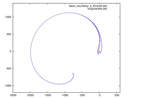
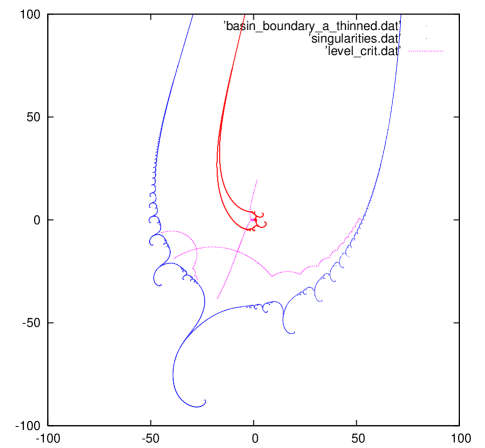
Figure 13. The domain of analyticity of $f_{*}$ and the boundary of the immediate parabolic basin $B_{0}^{f_{*}}$. In the second figure, a part of the critical level curve of $f_{*}$ is also indicated.

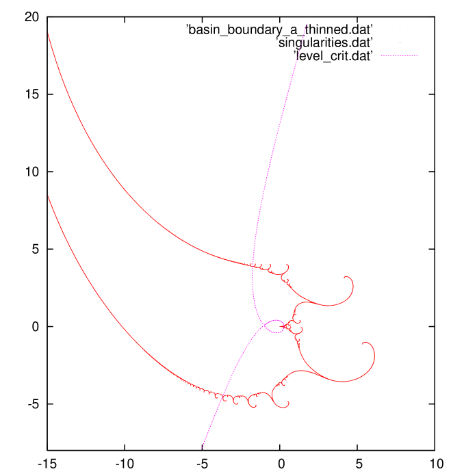
Figure 14. A blow-up of the boundary of the immediate basin of $f_{*}$ in the vicinity of the parabolic point.

The size of the domain of analyticity. To draw the pictures of the domain of analyticity of the fixed point of $f_{*}$ (Figures 13 and 14) we employed the following strategy. First, a periodic orbit of period $2$ in $\partial B_{0}$ was identified. Its preimages give a rough outline of $\partial B_{0}$, but become sparse near the “tails”, which are not visible in this initial outline. At the next step, the large “tail” of $B_{0}$ is computed as described above. Finally, its preimages are used to fill in the remaining gaps in $\partial B_{0}$.

As the final step, we calculate the boundary of $\operatorname{Dom}(f_{*})$ as

$$\partial\operatorname{Dom}(f_{*})=\operatorname{ixp}\circ\phi_{R}(\partial B_{0}\cap P_{R}).$$

An empirical estimate of the inner radius of $\text{Dom}(f_{*})$ around the origin allows us to formulate the following observation (see Figure 14):

Empirical Observation 5.5.

The radius of convergence of the Taylor’s expansion of $f_{*}$ at the origin is $R\approx 41.$

Appendix A Example of a map with a simply-connected parabolic basin whose boundary is not locally connected

Theorem A.1.

There exists a quadratic rational map $R:\hat{\mathbb{C}}\to\hat{\mathbb{C}}$ of degree $2$ with the following properties:

• $R$ has a simple parabolic fixed point at $\infty$ with a proper immediate basin $B_{0}^{R}$ of degree $2$;

• the boundary of the immediate basin $B_{0}^{R}$ is not locally connected.

We begin by recalling:

Proposition A.2.

There exist $\alpha\in{\mathbb{R}}/\setminus{\mathbb{Q}}$ such that no fixed point of multiplier $e^{2\pi i\alpha}$ for a rational function of degree $d$ can be locally linearizable.

The first proof of this result is due to Cremer [1927], who gave a sufficient condition for $\alpha$ (see [Mil1], Theorem 11.2).

Let us fix $\alpha$ as in Proposition A.2 and set $\lambda=e^{2\pi i\alpha}$.

Proposition A.3.

There exists a quadratic rational map $R$ with a simple parabolic point with multiplier $1$ at $\infty$, and a Cremer point with multiplier $\lambda$ at $0$.

Proof.

The reader may find a detailed discussion of the dynamics of quadratic rational maps in Milnor’s paper [Mil2]. Below we give a brief summary of some relevant facts. Every quadratic rational map $F$ has three fixed points, counted with multiplicity. Let $\mu_{1}$, $\mu_{2}$, $\mu_{3}$ denote the multipliers of the fixed points.

$$\sigma_{1}=\mu_{1}+\mu_{2}+\mu_{3},\;\sigma_{2}=\mu_{1}\mu_{2}+\mu_{1}\mu_{3}+\mu_{2}\mu_{3},\;\sigma_{3}=\mu_{1}\mu_{2}\mu_{3}$$

be the elementary symmetric functions of these multipliers.
Proposition ([Mil2], Lemma 3.1). The numbers $\sigma_{1}$, $\sigma_{2}$, $\sigma_{3}$ determine $F$ up to a Möbius conjugacy, and are subject only to the restriction that

$$\sigma_{3}=\sigma_{1}-2.$$

Hence the moduli space of quadratic rational maps up to Möbius conjugacy is canonically isomorphic to ${\mathbb{C}}^{2}$, with coordinates $\sigma_{1}$ and $\sigma_{2}$.

Note that for any choice of $\mu_{1}$, $\mu_{2}$ with $\mu_{1}\mu_{2}\neq 1$ there exists a quadratic rational map $F$, unique up to a Möbius conjugacy, which has distinct fixed points with these multipliers. The third multiplier can be computed as $\mu_{3}=(2-\mu_{1}-\mu_{2})/(1-\mu_{1}\mu_{2})$.

Thus there exists a quadratic rational map $R$ with fixed points at $0,\infty$ such that $R^{\prime}(0)=\lambda$ and $R^{\prime}(\infty)=1$. The map $R$ has only two critical orbits, and at least one of them has to contain the Cremer fixed point $0$ in its closure. Thus the parabolic basin of $\infty$ can contain only one critical value, and hence $\infty$ is a simple parabolic point.

∎

Let us fix $R$ as in Proposition A.3. The following is an immediate consequence of Montel’s Theorem:

Proposition A.4.

The Julia set

$$J(R)=\partial B_{0}^{R}.$$

Let us now argue by way of contradiction and assume that $\partial B_{0}^{R}$ is locally connected. It is elementary to see that $B_{0}^{R}$ is simply-connected. Denote $D:{\mathbb{T}}\to{\mathbb{T}}$ the doubling map $D(x)=2x\operatorname{mod}1$.

Proposition A.5.

There exists a continuous surjective map $\gamma:{\mathbb{T}}\to\partial B_{0}^{R}$ such that

$$\gamma\circ D=R\circ\gamma.$$

Proof.

We use the fact that $R$ is conformally conjugate to the Koebe function $K$ on the immediate basin $B_{0}^{R}$,

$$\psi\circ R\circ\psi^{-1}=K,$$

and apply Carathéodory Theorem to the conformal map $\psi$. ∎

Let us denote $W=\gamma^{-1}(0).$ We claim:

Proposition A.6.

The set of angles $\gamma$ is finite.

To prove this first note that $R$ is a local homeomorphism at $0$ and therefore it induces a homeomorphism on $W$. The proposition now follows from the following general fact (see e.g. [Mil1], Lemma 18.8):

Lemma A.7.

Let $X$ be a compact metric space and let $h:X\to X$ be a homeomorphism. If $h$ is expanding then $X$ is finite.

We conclude:

Corollary A.8.

There exists a periodic angle $x\in B$.

We are now set to prove Theorem A.1:

Proof.

Let $\psi$ be as in Proposition A.5 and let

$$\ell=\psi^{-1}({\mathbb{R}})\subset B_{0}^{R}.$$

Let us denote $U^{+}$, $U^{-}$ the components of $B_{0}^{R}\setminus\ell$. To fix the ideas, assume that the angle $x$ from Proposition A.8 corresponds to a prime end $p$ in the Carathéodory completion of $U^{+}$, and has period $m$ under the doubling map. Let $Q:U^{+}\to U^{+}$ be the branch of $R^{-m}$ whose Carathéodory extension fixes $p$. By Denjoy-Wolff Theorem, all orbits of $Q$ converge to $0$. Hence, $0$ has a non-empty basin under $Q$, and thus is either repelling or parabolic for $R$, which contradicts our assumptions. ∎

We finally note, that up to a conjugacy by $z\mapsto az$ with $a\in{\mathbb{C}}^{*}$, our map $R$ has the form

$$R(z)=\frac{z^{2}+\lambda z}{z+1}.$$

Appendix B Example of a map in ${{{{\mathbf{P}}}}}\setminus{{{{\mathbf{P}}}}_{0}}$.

We begin by showing:

Theorem B.1.

There exists a quadratic rational map $R$ with a simple parabolic fixed point whose immediate basin $B_{0}^{R}$ is simply connected and has a locally connected boundary, which is not a Jordan curve.

We find our example in the family of quadratic rational maps

$$R_{a}(z)=\frac{a}{z^{2}+2z}$$

which was considered in [AY]. For $a\neq 0$ the map $R_{a}$ has two simple critical points $c_{1}=-1$ and $c_{2}=\infty.$ The latter one is periodic with period 2:

$$\infty\mapsto 0\mapsto\infty.$$

Fix $a_{0}=32/27$ and let $R\equiv R_{a_{0}}$. The rational function $R$ has a parabolic fixed point $z_{0}=-\frac{4}{3}$ with multiplier $1$. Since there is a single critical orbit of $R$ which may be attracted by $z_{0}$, the point $z_{0}$ is a simple parabolic fixed point. Elementary considerations imply that $B_{0}^{R}$ is simply-connected, it is bounded since a neighborhood of $\infty$ belongs to the basin of the super-attracting cycle of period $2$.

By Montel’s Theorem $\partial B_{0}^{R}=J(R)$. The rational map $R$ can be described as a conformal mating of the basilica $z\mapsto z^{2}-1$ and the parabolic map $z\mapsto z+z^{2}$. The Julia set of $R$ is locally connected by [TY].

The other fixed point of $R$ is $\alpha=\frac{2}{3}$. It is repelling: $R^{\prime}(\alpha)=-\frac{5}{4}$. It is elementary to verify that the interval $[0,\alpha]$ is invariant under the second iterate of $R$, and that

$$R^{2}(x)<x\text{ for }x\in(0,\alpha).$$

Hence, the interval $(0,\alpha)$ belongs to the super-attracting basin, and so does the interval $(\alpha,\infty)$. The point $\alpha$ is on the boundary of the immediate basin $B_{0}^{R}$ and hence must be accessible from $B_{0}^{R}$. By real symmetry, $\alpha$ is bi-accessible from $B_{0}^{R}$. Consider the parabolic renormalization $F\equiv{\cal P}(R)$. Preimages of $\alpha$ are dense in $\partial B_{0}^{R}$, and therefore the boundary ${\cal D}(F)$ contains locally conformal preimages of a neighborhood of $\alpha$ in $J(R)$. In particular, $\partial{\cal D}(F)$ contains bi-accessible points, and therefore is not Jordan. On the other hand, $\partial{\cal D}(F)$ is a locally homeomorphic image of a locally connected set, and hence is locally connected. Thus, $F\in{{{{\mathbf{P}}}}}\setminus{{{{\mathbf{P}}}}_{0}}$. Note that by Theorem 4.9, the parabolic renormalization ${\cal P}(F)\in{{{{\mathbf{P}}}}_{0}}.$

References

- [AY] M. Aspenberg, M. Yampolsky. Mating non-renormalizable quadratic polynomials, Commun. Math. Phys., 287(2009), p.1-40
- [BE] X. Buff, A. Epstein. A parabolic Pommerenke-Levin-Yoccoz inequality. Fund. Math. 172, no 3.(2002), 249-289
- [BH] X. Buff, J.H. Hubbard. Dynamics in One Complex Variable. Manuscript.
- [Co] J. B. Conway. Functions of One Complex Variable II. Graduate Texts in Mathematics 159. Springer-Verlag, 1995
- [Do1] A. Douady, Systéms dynamiques holomorphes, Seminar Bourbaki, Astérisque, 105-106 (1983) 39-64.
- [Do2] A. Douady. Does a Julia set depend continuously on the polynomial? In Complex dynamical systems: The mathematics behind the Mandelbrot set and Julia sets. ed. R.L. Devaney, Proc. of Symposia in Applied Math., Vol 49, Amer. Math. Soc., 1994, pp. 91-138.
- [DH] A. Douady, J.H. Hubbard. Etude dynamique des polynômes complexes, I-II. Pub. Math. d’Orsay, 1984.
- [Du] A. Dudko. Dynamics of holomorphic maps: Resurgence of Fatou coordinates, and Poly-time computability of Julia sets. PhD Thesis, University of Toronto, 2012.
- [DS] A. Dudko, D. Sauzin. Écalle-Voronin invariants via resurgence. Manuscript in preparation, 2011.
- [Ec] J. Écalle. Les fonctions résurgentes, Publ. Math. d’Orsay [Vol. 1: 81-05, Vol. 2: 81-06, Vol. 3: 85-05] 1981, 1985
- [Ep] A. Epstein, Towers of finite type complex analytic maps. PhD Thesis, CUNY, 1993.
- [EKT] A. Epstein, L. Keen, C. Tresser. The set of maps with any given rotation interval is contractible. Commun. Math. Phys. 173, 313-333, 1995.
- [EY] A. Epstein, M. Yampolsky. The universal parabolic map. Accepted to Ergodic Th. & Dynam. Sys., available from http://www.math.toronto.edu/yampol
- [IS] H. Inou and M. Shishikura. The renormalization for parabolic fixed points and their perturbation. Preprint, 2008.
- [Lan] O.E. Lanford. The zero rotation number fixed point. Manuscript.
- [Lav] P. Lavaurs. Systémes dynamiques holomorphes: Explosion de points périodiques, Thèse, Université de Paris-Sud, 1989.
- [Lyu] M. Lyubich. The dynamics of rational transforms: the topological picture. Russian Math. Surveys 41:4(1986), 43-117.
- [Mil1] J. Milnor. Dynamics in One Complex Variable. 3rd ed. Annals of Math. Studies 160. Princeton University Press, 2006
- [Mil2] J. Milnor, Geometry and dynamics of quadratic rational maps, Experim. Math., 2 (1993) 37-83.
- [Mil3] J. Milnor, Pasting together Julia sets - a worked out example of mating, Experiment. Math. 13(2004), no. 1, 55–92.
- [Ram] J.-P. Ramis. Séries divergentes et théories asymptotiques, Panoramas et Synthèses (1994)
- [Sau] D. Sauzin. Resurgent functions and splitting problems. RIMS Kokyuroku 1493, p. 48-117, 2005 available from http://www.imcce.fr/Equipes/ASD/person/Sauzin/sauzpreprint.php
- [Sh] M. Shishikura. The Hausdorff dimension of the boundary of the Mandelbrot set and Julia sets. Ann. of Math. (2) 147(1998), no. 2, 225-267.
- [TY] L. Tan, Y. Yin, Local connectivity of the Julia set for geometrically finite rational maps, Science in China (Serie A) 39 (1996), 39 47.
- [Vor] S.M. Voronin. Analytic classification of germs of conformal maps with identity linear part. Funct. Anal. Appl., 15(1981), 1-17.
- [Ya] M. Yampolsky. The attractor of renormalization and rigidity of towers of critical circle maps, Commun. Math. Phys., 218(2001), no. 3, 537-568.
- [YZ] M. Yampolsky, S. Zakeri. Mating Siegel quadratic polynomials, Journ. Amer. Math. Soc., 14(2000), 25-78