Lattice oscillator model, scattering theory and a many-body problem

Abstract

We propose a model for the quantum harmonic oscillator on a discrete lattice which can be written in supersymmetric form, in contrast with the more direct discretization of the harmonic oscillator. Its ground state is easily found to be annihilated by the annihilation operator defined here, and its excitation spectrum is obtained numerically. We then define an operator whose continuum limit corresponds to an angular momentum, in terms of the creation-annihilation operators of our model. Coherent states with the correct continuum limit are also constructed. The versatility of the model is then used to calculate, in a simple way, the generalized position-dependent scattering length for a particle colliding with a single static impurity in a periodic potential and the exact ground state of an interacting many-body problem in a one-dimensional ring.

1 Introduction

The quantum harmonic oscillator is a paradigmatic model with applications in all branches of physics, too numerous to be counted. Due to the special structure of its Hamiltonian, it is possible to obtain its eigenstates exactly in several different ways. Perhaps the most celebrated one is the algebraic solution by means of the creation-annihilation (ladder) operators [1], which is by far the simplest and most elegant and, moreover, it is the first step towards field quantization [2].

For more complicated problems the use of numerical methods becomes necessary. One of the most popular techniques is the finite-difference discretization, which is often employed in high-energy physics to obtain non-perturbative results [3]. However, this method has severe problems, since the symmetries of the original problem are usually lost on the lattice and can only be recovered once the continuum limit is taken which, in practice, is numerically impossible. As an important example, the lattice harmonic oscillator, though it can be written as the Mathieu equation in quasi-momentum space [4, 5], is not factorizable and not even its ground state can be obtained in closed form. This fact is very disappointing, since then the supersymmetric (SUSY) structure of the system is not transparent – in fact, not even present – until the continuum limit is taken.

In this article, we construct a model for the lattice harmonic oscillator which has a correct continuum limit. Its Hamiltonian is shape invariant [1] and, though the excitations cannot be accessed analytically, its ground state is exactly solvable for any value of the oscillator frequency and the lattice spacing. The excitations can, however, be obtained by solving an equation which is analogous to the Hermite equation. We propose then a definition of coherent states, finding that their correct continuum limit cannot be obtained if they are defined as eigenstates of the lattice annihilation operators, so their definition has to be given in terms of the displacement operator. Our model is completely analogous to that for a single particle in a periodic potential, and we use it to calculate the lowest band zero energy scattering length in a particle-impurity collision. We then make further use of the analogy of the model with a many-body system with anharmonic interactions on a finite ring which can be solved exactly for the ground state.

2 Position and momentum operators on the lattice

We define the following operators in quasi-momentum space as the momentum ($\hat{p}$) and position ($\hat{x}$) operators,

$$\hat{p} \equiv\frac{\hbar}{d}\sin{kd}$$ (1)

$$\hat{x} \equiv\mathrm{i}\frac{\partial}{\partial k},$$ (2)

where $d$ ($>0$) is the lattice spacing and $k\in(-\pi/d,\pi/d]$ is the quasi-momentum. The operators $\hat{p}$ and $\hat{x}$ are constructed in analogy with their continuous space counterparts. Note that $\hat{x}$ coincides with its continuum analog while $\hat{p}=\hbar k+O(d^{2})$ as $d\to 0$, and therefore their continuum limits are correctly described. We can write the lattice analog of the harmonic oscillator annihilation $\hat{a}$ and creation $\hat{a}^{\dagger}$ operators as

$$\hat{a} =(\hat{X}+\mathrm{i}\hat{P})/\sqrt{2}$$ (3)

$$\hat{a}^{\dagger} =(\hat{X}-\mathrm{i}\hat{P})/\sqrt{2},$$ (4)

where the quadrature operators are defined as

$$\hat{X} \equiv(m\omega/\hbar)^{1/2}\hat{x},$$ (5)

$$\hat{P} \equiv(m\hbar\omega)^{-1/2}\hat{p}.$$ (6)

However, by using the lattice operators of Eqs. (1) and (2) we see that $[\hat{X},\hat{P}]=\mathrm{i}\cos(kd)$ and $[\hat{a},\hat{a}^{\dagger}]=\cos(kd)$. In other words, the canonic commutation relations are valid up to a factor of $\cos(kd)$. In the limit of small lattice spacing, we obtain the correct commutation relation of the continuous space case $\lim_{d\to 0}[\hat{X},\hat{P}]=\mathrm{i}$. The commutation relation $[\hat{X},\hat{P}]$ yields a generalized uncertainty principle (GUP) [6] of the form

$$\Delta X\Delta P\geq\frac{1}{2}|\langle\cos(kd)\rangle|,$$ (7)

which resembles the GUP of systems with a minimal length [7]. The GUP (7) does not imply any minimal $\Delta X$ (it can be zero). However, we have a maximal dispersion for the momentum,

$$\Delta P\leq\Delta P_{\mathrm{max}}=\sqrt{\frac{\hbar\pi}{m\omega d^{3}}},$$ (8)

which is infinite in the continuum limit, as it should.

3 The lattice harmonic oscillator

If we wish to construct a lattice theory for the harmonic oscillator having a similar structure as its continuum limit, we have to consider the operator

$$\hat{N}\equiv\hat{a}^{\dagger}\hat{a}=\frac{1}{2}(\hat{P}^{2}+\hat{X}^{2}+\mathrm{i}[\hat{X},\hat{P}]).$$ (9)

So far, the “number” operator, Eq. (9), has exactly the same appearance as in continuous space. Its explicit form is given by

$$\hat{N}=\frac{1}{2}\left(-\frac{m\omega}{\hbar}\frac{\partial^{2}}{\partial k^{2}}+\frac{\hbar}{m\omega d^{2}}\sin^{2}(kd)-\cos(kd)\right).$$ (10)

The number operator written in this way looks rather unusual. If we rewrite $\sin^{2}(kd)=(1-\cos(2kd))/2$, and perform Fourier transform to direct lattice space, then we see that the number operator $\hat{N}$ acts as

$$(\hat{N}\psi)(x) =\frac{1}{2}\big{[}\frac{m\omega}{\hbar}x^{2}\psi(x)-\frac{\psi(x+d)+\psi(x-d)}{2}$$ (11)

$$+\frac{\hbar}{2m\omega d^{2}}\big{(}\psi(x)-\frac{\psi(x+2d)+\psi(x-2d)}{2}\big{)}\big{]}$$

where $n=x/d\in\mathbb{Z}$ are the lattice points. Thus, the number operator corresponds to a lattice with nearest-neighbor and next-nearest-neighbor hoppings with an external harmonic trap, plus a trivial constant. After taking the continuum limit $d\to 0$, one easily verifies that $\hbar\omega\hat{N}\to\hat{p}^{2}/2m+m\omega^{2}x^{2}/2-\hbar\omega/2$.

3.1 Ground state and lattice Hermite equation

From now on we consider the Hamiltonian

$$H\equiv\hbar\omega\big{(}\hat{N}+\frac{1}{2}\big{)}.$$ (12)

If operator $\hat{a}$ annihilates a wave function in $k$-space which is $2\pi$-periodic,[8] then it is the ground state of $H$ with energy $E_{0}=\hbar\omega/2$. Equation $\hat{a}\psi_{0}(k)=0$ is readily solved and the ground state wave function has the form

$$\psi_{0}(k)=\mathcal{N}e^{-\gamma_{d}}e^{\gamma_{d}\cos(kd)},$$ (13)

where $\gamma_{d}\equiv\hbar/(m\omega d^{2})$. In the continuum limit, Eq. (13) reduces to the well-known harmonic oscillator ground state, $\psi_{0}(k)\sim\exp(-\hbar k^{2}/m\omega)$. We use this result to verify the uncertainty principle on the lattice, and find that in the ground state of the lattice harmonic oscillator, the uncertainty relation is also minimal,

$$\Delta X\Delta P=\frac{1}{2}\left|\frac{\langle\psi_{0}|\,\cos(kd)\,|\psi_{0}\rangle}{\langle\psi_{0}|\psi_{0}\rangle}\right|,$$ (14)

since in general $\Delta X\Delta P\geq|\langle\big{[}\hat{X},\hat{P}\big{]}\rangle|/2$.

Further analogy with the harmonic oscillator in continuous space can be observed by solving the eigenvalue problem for the number operator $\hat{N}\psi(k)=\tilde{N}\psi(k)$ with the ansatz $\psi(k)=\psi_{0}(k)\phi(k)$. The eigenvalue problem is then transformed to the equation

$$\phi^{\prime\prime}(k)-2\frac{\hbar}{m\omega}\frac{\sin(kd)}{d}\phi^{\prime}(k)+2\frac{\hbar}{m\omega}\tilde{N}\phi(k)=0$$ (15)

that determines the unknown $\phi(k)$ for which periodic boundary conditions (PBC) $\phi(k+2\pi/d)=\phi(k)$ are assumed. Note the analogy of Eq. (15) with the Hermite equation: the naive substitution $\sin(kd)/d\sim k$, valid for $kd\ll 1$, yields the well-known continuum limit, in which the eigenvalues $\tilde{N}$ become natural numbers.

In Fig. 1 we plot the low-energy eigenvalues $\tilde{N}$ of $\hat{N}$, Eq. (10), for a small value of the lattice spacing $d$. We see that the lowest eigenvalue is indeed zero, while the rest of the eigenvalues appear to be quasi-degenerate but almost linearly spaced as $\tilde{N}_{s+2}-\tilde{N}_{s}=1$. The reason is that, in direct lattice space, the number operator includes tunneling to nearest and second nearest neighbors, therefore inducing the quasi-degeneracy, except for the ground state. The relevant eigenstates for the continuum limit are those labeled by even quantum numbers $s$ and, in direct lattice space, appear to be essentially a superposition of the discretized Hermite functions $\psi_{s/2}(x=2nd)-\psi_{s/2}(x=-(2n+1)d)$.

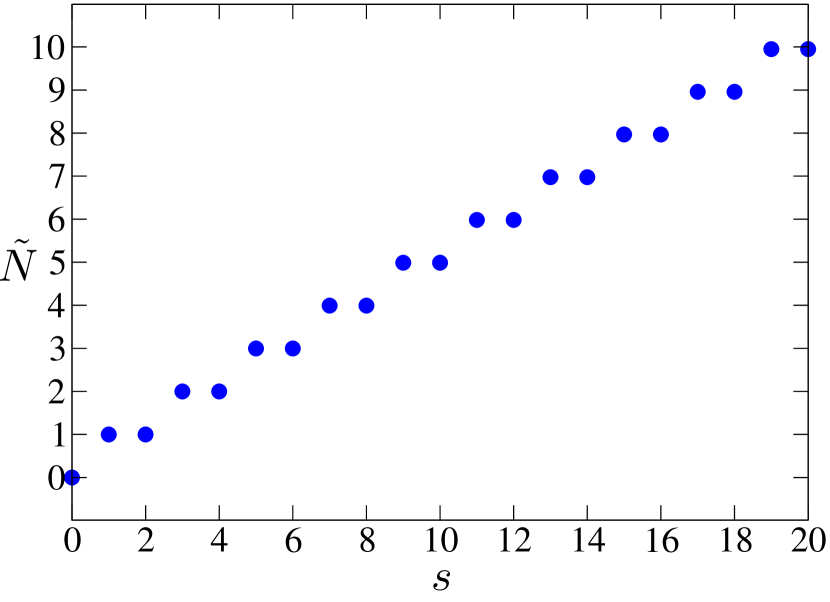
Figure 1: Eigenvalues of $\hat{N}$, Eq. (10), for $d=\frac{1}{10\sqrt{5}}\sqrt{\frac{\hbar}{m\omega}}$.

3.2 Coherent states

It is natural to define now the coherent states for the lattice harmonic oscillator. First, we try the eigenstates of the annihilation operator, $\hat{a}\psi_{\alpha}=\alpha\psi_{\alpha}$, with $\alpha\in\mathbb{C}$. The solution of this equation is

$$\psi_{\alpha}(k)=\exp\left[-\mathrm{i}2\sqrt{\frac{\hbar}{m\omega}}\alpha k\right]\psi_{0}(k)$$ (16)

with $\psi_{0}(k)$ being the ground state, Eq. (13). If we assumed $\alpha$ to be any complex number, $\psi_{\alpha}$ would not fulfill the PBC. Hence, if we insist on $\psi_{\alpha}$ to be correct, we have no choice but to restrict the values of $\alpha$ to $\alpha_{j}=\frac{1}{2}\sqrt{\frac{m\omega}{\hbar}}j,\hskip 5.69046ptj\in\mathbb{Z}$, which is a very unsatisfactory answer since the coherent states would then be restricted to equally spaced real numbers. Therefore the coherent states $\psi_{\alpha}$ do not present a very convenient definition. This apparently difficult situation can be resolved in a rather elegant way, however, relaxing the requirement that the coherent states be eigenstates of the lattice annihilation operator $\hat{a}$. To this end, we define the coherent states $\Psi_{\alpha}$ as solutions of the equation $\hat{a}\Psi_{\alpha}(k)=\alpha\cos(kd)\Psi_{\alpha}(k)$,

$$\Psi_{\alpha}(k)=\exp\left[-\mathrm{i}2\alpha\sqrt{\frac{\hbar}{m\omega}}\frac{\sin(kd)}{d}\right]\psi_{0}(k),$$ (17)

which are obviously $2\pi$-periodic for all $\alpha\in\mathbb{C}$, and have the correct continuum limit. We can further justify Eq. (17) as a definition since even in the continuum the coherent states are solutions of $(\hat{a}+\alpha\mathrm{i}[\hat{X},\hat{P}])\Psi_{\alpha}=0$. The only issue we cannot generalize to the lattice case is the usual form of the displacement operator, since on the lattice the Baker-Hausdorff formula is not valid due to the commutator $\big{[}\hat{a},[\hat{a},\hat{a}^{\dagger}]\big{]}\neq 0$. Therefore we define here the displacement (or translation) operator for lattice and continuum as $\hat{D}(\alpha)=e^{-\mathrm{i}2\alpha\hat{P}}$, which generates unnormalized coherent states.

3.3 Angular momentum

A major inconvenience of lattice discretizations, if these are introduced artificially and not due to a true underlying crystal structure, is the absence of continuous rotational symmetry. To be more concrete, we lack conservation of angular momentum or, more dramatically, we do not even have a definition of angular momentum on the lattice!

We propose here a rather simple lattice analog of the angular momentum. The requirements this operator has to satisfy are rather relaxed: (i) it should have a correct continuum limit, (ii) there should be a ground state of some relevant enough Hamiltonian with a well defined “angular momentum” on the lattice and, (iii) the lattice angular momentum cannot commute with the lattice Hamiltonian. Requirement (iii) is easy to satisfy: take any Hamiltonian which respects the symmetries of the lattice. We discuss now how (i) and (ii) can be met. Consider first a two-dimensional (2D) oscillator with Hamiltonian $H^{(\mathrm{2D})}=\hbar\omega\big{[}\hat{N}_{1}+\hat{N}_{2}+1]$, with $\hat{N}_{i}=\hat{a}^{\dagger}_{i}\hat{a}_{i}$. We define the lattice angular momentum in 2D, in analogy with the continuum, as

$$\hat{L}\equiv\hat{x}_{1}\hat{p}_{2}-\hat{x}_{2}\hat{p}_{1}=\mathrm{i}(\hat{a}_{1}\hat{a}^{\dagger}_{2}-\hat{a}^{\dagger}_{1}\hat{a}_{2}),$$ (18)

and we see that condition (i) is fulfilled. As promised, requirement (ii) is automatically satisfied by the ground state of $H^{(\mathrm{2D})}$, $\psi_{0}^{(\mathrm{2D})}(k_{1},k_{2})=\psi_{0}(k_{1})\psi_{0}(k_{2})$, with $\psi_{0}(k_{i})$ defined in Eq. (13), and by the ground state of the 2D free particle Hamiltonian $H_{F}=-2J\sum_{k_{1},k_{2}}(\cos(k_{1}d)+\cos(k_{2}d))\,|k_{1},k_{2}\rangle\langle k_{1},k_{2}|\,$, $\psi(k_{1},k_{2})=\delta(k_{1})\delta(k_{2})$, both having angular momentum $L=0$ as a good quantum number. It must be noted that lattice angular momentum operators have been defined in the context of rotating gases in an optical lattice in [9], but with such definition requirement (ii) is no longer satisfied for the ground state of the lattice oscillator. We now show by explicit calculation that the angular momentum on the lattice is in general not a conserved quantity

$$[\hat{L},\hat{N}_{1}+\hat{N}_{2}]= \mathrm{i}\big{[}\cos(k_{1}d)\hat{a}_{1}\hat{a}^{\dagger}_{2}+\hat{a}_{2}\hat{a}^{\dagger}_{1}\cos(k_{1}d)$$ (19)

$$-\hat{a}_{1}\hat{a}^{\dagger}_{2}\cos(k_{2}d)-\cos(k_{2}d)\hat{a}_{2}\hat{a}^{\dagger}_{1}\big{]},$$

which, as expected, is non-zero, but vanishes in the continuum limit. It must be noted now that the lattice angular momentum operator, Eq. (18), can be used as a definition not only for the model discussed here, but for any tight-binding lattice model even without next-nearest-neighbor hopping.

4 Application to impurity scattering in a periodic potential

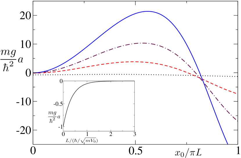
Figure 2: Scattering lengths for $mV_{0}L^{2}/\hbar^{2}=10^{-3}$, $1/2$, $1$ and $3/2$ (at $x_{0}=0$ from bottom to top). Inset: $a(0)$ as a function of $L$.

The model presented here can be applied to construct completely different systems and obtain some of their properties exactly. As a first application, let us consider a single particle moving on the real line. It is readily verified that the Hamiltonian with the periodic potential,

$$V(x)=V_{0}\sin^{2}(x/L)-\frac{\hbar}{L}\sqrt{\frac{V_{0}}{2m}}\cos(x/L)$$ (20)

has a ground state $\psi_{0}(x)=\exp[\lambda_{L}\cos(x/L)]$, with $\lambda_{L}=\sqrt{2mV_{0}}L/\hbar$, since the potential and kinetic energy operators are dual to those for the lattice Harmonic oscillator in quasi-momentum space. We consider a single static impurity located at $x_{0}\in(-\pi L,\pi L]$ (this is the central site, and by translation applies to an impurity at any site), with zero range interaction potential $V_{g}(x)=g\delta(x-x_{0})$, and we show how to get the low-energy scattering properties of the system in a very simple manner. First we notice that, since $V$ has a purely continuous spectrum and the impurity is immobile, upon collision the incident waves can only acquire a phase shift. Therefore, for low-energy scattering we only need the periodic ($\psi_{0}$) and aperiodic (which we call $\psi_{I}$) solutions for zero energy. The aperiodic solution centered at the first site is given by

$$\psi_{I}(x)=\psi_{0}(x)\int^{x}dxe^{-2\lambda_{L}\cos(x/L)}\equiv\psi_{0}(x)\Phi(x).$$ (21)

This aperiodic solution is clearly antisymmetric and it holds that $\Phi(x)=\beta x+\phi_{p}(x)$, where $\phi_{p}(x+2\pi L)=\phi_{p}(x)$. Recall that without the periodic potential, this solution corresponds to setting $\phi_{p}\equiv 0$, and the scattering length $a_{0}$ of a static Dirac delta impurity is defined [10] by the zero-energy solution $f_{0}(x)=1-|x|/a_{0}$. Clearly, $f_{0}$ is the sum of the periodic (free) solution and the aperiodic (unnormalizable) solution, with the inverse scattering length as a coefficient. In analogy to the free space situation, we define a position-dependent scattering length $a(x_{0})$, $x_{0}\in(-\pi L,\pi L]$, in terms of the zero-energy solution

$$f(x;x_{0})=\psi_{0}(x)-\frac{|\psi_{I}(x)-\psi_{I}(x_{0})|}{a(x_{0})},$$ (22)

which, written in this way, satisfies the boundary condition

$$f^{\prime}(x_{0}^{+})-f^{\prime}(x_{0}^{-})=2mgf(x_{0})/\hbar^{2}$$ (23)

imposed by the Dirac delta, if

$$a(x_{0})=-\frac{\hbar^{2}}{mg}\left[\frac{\left(\psi_{0}\Phi\right)^{\prime}}{\psi_{0}}\right]_{x=x_{0}}$$ (24)

for $x_{0}\in(-\pi L,\pi L]$, and $a(x_{0}+n2\pi L)=a(x_{0})$, with $n\in\mathbb{Z}$. In the simplest case of $x_{0}=0$, the scattering length is shown to have the form $a(0)=-\hbar^{2}e^{-2\lambda_{L}}/(mg)$. If $x_{0}\neq 0$ it has to be calculated numerically. In Fig. 2 we plot the scattering length $a(x_{0})$, showing how strongly it depends on the position of the impurity. The scattering length never diverges (there is no resonance), but $mga(x_{0})/\hbar^{2}$ can actually become positive and indeed very large with increasing $V_{0}$ at $x_{0}\neq 0$, even though the corresponding free-space scattering length (we assume $g>0$) is negative. This means that interactions in a periodic potential can effectively change both quantitative and qualitatively, depending on where the scattering takes place.

5 A many-body system

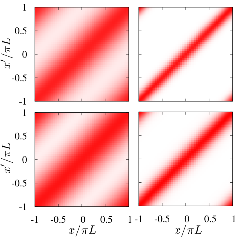
Figure 3: Pair correlation functions $\rho(x,x^{\prime})$; the clearer the color the lower its value. Top $N=4$ particles, bottom $N=2$ particles. Left $\lambda L^{2}=0.1$, right $\lambda L^{2}=1$. All values are normalized to the peak.

As a second application, we construct a many-body Hamiltonian of interacting particles on a finite ring whose ground state can be obtained in closed form. We consider $N$ particles on a ring of length $2\pi L$. The position of particle $i\in\{1,\ldots,N\}$ is denoted by $x_{i}\in(-\pi/L,\pi L]$ and its momentum by $p_{i}=-\mathrm{i}\hbar\partial/\partial x_{i}$, and for all the functions involved we use PBC. We consider the following Hamiltonian

$$H =\frac{\hbar^{2}}{2m}\sum_{i=1}^{N}\hat{A}_{i}^{\dagger}\hat{A}_{i},$$ (25)

$$\hat{A}_{i} =\frac{\partial}{\partial x_{i}}+\lambda L\sum_{j=1,j\neq i}^{N}\sin(x_{i,j}/L),$$ (26)

where $x_{i,j}=x_{i}-x_{j}$. With these definitions, the many-body Hamiltonian (25) is $2\pi$-periodic. In the limit of an infinitely long ring, $L\to\infty$, we are left with $N$ particles interacting via pairwise harmonic potentials. However, for any finite-size ring the interactions are anharmonic and contain three-body terms.

Since the Hamiltonian $H$, Eq. (25), is the sum of semi-positive operators, it follows that $H\geq 0$. Hence, if there exists a non-singular periodic function $\psi_{0}$ which is annihilated by all $A_{i}$, $i=1,\ldots,N$, then it is the ground state of $H$ and its eigenenergy is zero. The set of $N$ equations $\hat{A}_{i}\psi_{0}=0$ is easily shown to be satisfied by the wave function

$$\psi_{0}(x_{1},\ldots,x_{N})=\mathcal{N}\prod_{i<j=1}^{N}\exp\Big{[}2\lambda L^{2}\cos(x_{i,j}/L)\Big{]},$$ (27)

with $\mathcal{N}$ the normalization constant. It is remarkable that for any $L<\infty$, the ground state (27) is square integrable, even if $\lambda<0$, but in taking the limit of $L\to\infty$ this will no longer be true.

In Fig. 3 we plot some ground state pair correlation functions, defined as

$$\rho(x,x^{\prime})\propto\int_{\Omega}dx_{3}\ldots dx_{N}|\psi_{0}(x,x^{\prime},\ldots,x_{N})|^{2},$$ (28)

where $\Omega\equiv(-\pi/L,\pi/L]^{N-2}$. We note that as $\lambda L^{2}$($>0$) becomes larger, the particles tend to be tighter co-localized, which also happens for increasing number of particles.

6 Conclusions

We have constructed a lattice model of the harmonic oscillator with a correct continuum limit whose properties, especially in the ground state, are the perfect analogous of those in continuous space. We have also defined lattice coherent states and a lattice “angular momentum” in terms of the creation and annihilation operators of the model. By establishing connections with other systems, we were able to describe low-energy scattering in a periodic potential and an anharmonically interacting many-body system. These results are relevant for lattice simulations, cold collisions, many-body theory and quantum information [11, 12].

References

References

- [1] F. Cooper, A. Khare and U. Sukhatme, Phys. Rep. 251, 267 (1995).
- [2] A. Messiah, Quantum Mechanics (Dover, 1999).
- [3] H.J. Rothe, Lattice Gauge Theories, An Introduction (Cambridge University Press 2005).
- [4] E. Chalbaud, J.-P. Gallinar and G. Mata, J. Phys. A 19, L385 (1986).
- [5] D.C. Mattis, Rev. Mod. Phys. 58, 361 (1986).
- [6] A.F. Ali, S. Das and E.C. Vagenas, Phys. Lett. B 678, 497 (2009); S. Das, E.C. Vagenas and A.F. Ali, ibid. 690, 407 (2010).
- [7] S. Hossenfelder, Quantum Grav. 23, 1815 (2006).
- [8] For simplicity, we will call a function -periodic when it is actually -periodic.
- [9] R. Bhat et al., Phys. Rev. A 74, 063606 (2006).
- [10] E.H. Lieb, R. Seiringer, J.P. Solovej and J. Yngvason, The Mathematics of the Bose Gas and its Condensation (Birkhäuser, 2005).
- [11] M.A. Marchiolli, M. Ruzzi and D. Galetti, Phys. Rev. A 76, 032102 (2007).
- [12] P.E.M.F. Mendoça, R.d.J. Napolitano, M.A. Marchiolli, C.J. Foster and Y.-C. Liang, Phys. Rev. A 78, 052330 (2008).