Coronal radiation of a cusp of spun-up stars and the X-ray luminosity of Sgr A*

Abstract

Chandra has detected optically thin, thermal X-ray emission with a size of $\sim 1$ arcsec and luminosity $\sim 10^{33}$ erg s^-1 from the direction of the Galactic supermassive black hole (SMBH), Sgr A*. We suggest that a significant or even dominant fraction of this signal may be produced by several thousand late-type main-sequence stars that possibly hide in the central $\sim 0.1$ pc region of the Galaxy. As a result of tidal spin-ups caused by close encounters with other stars and stellar remnants, these stars should be rapidly rotating and hence have hot coronae, emitting copious amounts of X-ray emission with temperatures $kT\hbox{\hbox to0.0pt{\hbox{\lower 4.0pt\hbox{$\sim$}}\hss}\hbox{$<$}}$ a few keV. The Chandra data thus place an interesting upper limit on the space density of (currently unobservable) low-mass main-sequence stars near Sgr A*. This bound is close to and consistent with current constraints on the central stellar cusp provided by infrared observations. If coronally active stars do provide a significant fraction of the X-ray luminosity of Sgr A*, it should be moderately variable on hourly and daily time scales due to giant flares occurring on different stars. Another consequence is that the quiescent X-ray luminosity and accretion rate of the SMBH are yet lower than believed before.

1 Introduction

Our Galactic nucleus with its supermassive black hole (SMBH) of mass $M_{\rm{BH}}\approx 4\times 10^{6}$ $M_{\odot}$ is a subject of intensive studies in radio, submillimeter, infrared, X-ray and gamma-ray bands (see Genzel, Eisenhauer, & Gillessen 2010 for a recent review). The Chandra X-Ray Observatory, with its excellent spatial resolution (Weisskopf et al., 2002), has revealed a rich variety of compact and diffuse X-ray sources in the central square degree of the Milky Way (Muno et al., 2004; Wang, Dong, & Lang, 2006; Muno et al., 2008, 2009). One of the most interesting findings is the detection of faint extended X-ray emission surrounding the radiosource Sgr A* associated with the SMBH (Baganoff et al. 2003, hereafter B03). The X-ray source has a radius of only $\sim 1$”, or $\sim 0.04$ pc for a Galactic Centre (GC) distance of $\sim 8$ kpc. Its X-ray luminosity is few $10^{33}$ erg s^-1, and the spectrum is consistent with thermal emission from optically thin $kT\sim 1$–4 keV plasma, absorbed by a column $N_{\rm{H}}\sim 10^{23}$ cm^-2 of neutral gas (B03). This column density is roughly consistent with the interstellar extinction towards the GC region.

The currently favoured view is that the X-ray emission from the central arcsecond around Sgr A* is truly diffuse and associated with hot gas flowing towards the central SMBH (Quataert 2002; B03; Yuan, Quataert, & Narayan 2003; Cuadra et al. 2006; Xu et al. 2006). According to this scenario, the X-ray luminosity is dominated by thermal gas emission near the Bondi radius, $R_{\rm{B}}=GM_{\rm{BH}}/c_{\rm{s}}^{2}\sim 0.05$ pc (where $c_{\rm{s}}$ is the gas sound speed, corresponding to a temperature of a few $10^{7}$ K). The Chandra observations imply that the outer inflow rate is $\dot{M}_{\rm{out}}\sim 10^{-5}M_{\odot}$ yr^-1. Although this rate is very low compared to active galactic nuclei, if the SMBH were accreting gas at this rate in radiatively efficient mode its bolometric luminosity would be several $\times 10^{40}$ erg s^-1, i.e. 5 orders of magnitude higher than the total luminosity of Sgr A* (predominantly emitted at radio to submillimeter wavelengths). The radiative output can be much lower in the case of an advection-dominated accretion flow (ADAF). However, there is an additional problem that if all of the gas captured at $R_{\rm{B}}$ with rate $\dot{M}_{\rm{out}}$ were flowing towards the SMBH, that would contradict an upper limit on the gas density in the inner regions imposed by measurements of Faraday rotation in the direction of Sgr A*, which imply that $\dot{M}_{\rm{in}}\hbox{\hbox to0.0pt{\hbox{\lower 4.0pt\hbox{$\sim$}}\hss}\hbox{$<$}}10^{-7}M_{\odot}$ yr ^-1 (e.g. Bower et al. 2003). Largely to circumvent this problem, radiatively inefficient accretion flow (RIAF) models have been proposed for Sgr A*, in which very little mass available at large radii actually accretes onto the black hole (e.g. Yuan, Quataert, & Narayan 2003). To summarise, the question of gas accretion onto the SMBH in the GC remains an open and hotly debated issue.

B03 also discussed the alternative possibility of the extended X-ray emission from Sgr A* being the sum of a large number of point X-ray sources. However, these authors could not suggest good candidates for being such objects. Below, we revisit this hypothesis and suggest that combined emission of a few thousand late-type main-sequence (MS) stars may contribute significantly to or even dominate the X-ray emission from the vicinity of Sgr A*.

The GC stellar cluster is the densest concentration of stars in the Milky Way. There are few $10^{5}M_{\odot}$ of stars within $0.25$ pc of Sgr A*, with the space density of massive ($\mathrel{\hbox{\hbox to0.0pt{\hbox{\lower 4.0pt\hbox{$\sim$}}\hss}\hbox{$>$}}}10M_{\odot}$) stars rising inwards down to the smallest resolvable projected distances of $\sim 0.005$ pc from the SMBH (see Alexander 2005; Genzel, Eisenhauer, & Gillessen 2010 for reviews). If the space density of presumably much more numerous late-type MS stars behaves similarly, many of these should be rapidly rotating as a result of repeated tidal spin-ups caused by close encounters with other stars and stellar remnants (Alexander & Kumar 2001, hereafter AK01). We pursue this idea further by pointing out that fast rotation in stars with outer convective zones is always associated with strong coronal activity and greatly enhanced X-ray emission. Hence, if there is indeed a high-density cusp of late-type MS stars in the GC, which could be verified by near-infrared (NIR) observations with future extremely large telescopes, their cumulative coronal radiation can be responsible for a significant fraction of the X-ray emission from the vicinity of Sgr A*.

2 The model

AK01 estimated typical rotational velocities that stars in a GC stellar cusp can acquire over their lifespans as a result of repeated tidal interactions. We use their results to calculate the rotational evolution of stars. In addition, we take into account a counteracting effect – magnetic braking of stellar rotation.

2.1 The stellar cusp near the Galactic SMBH

The key question and major source of uncertainty for this study is how many late-type MS stars are present near Sgr A*. Unfortunately, NIR observations cannot yet provide a direct answer, since Sun-like stars are too faint and probably too densely clustered in the Galactic nucleus to be detected and individually resolved by present-day 8–10 meter telescopes.

High spatial resolution NIR observations, which currently can reliably resolve individual stars brighter than $K\sim 17$ in the GC region, have demonstrated that the space density of such bright stars increases inwards as $\rho_{\ast}(r)\propto r^{-\gamma}$, with $\gamma\approx 1.2$, in the innermost $\sim 0.25$ pc, whereas the slope steepens to $\gamma\approx 1.75$ at larger distances (Schödel et al. 2007; the actual slope of the nuclear cluster is inferred to be yet steeper once the contribution of the Galactic bulge to stellar counts is taken into account, Graham & Spitler 2009). Given the limit $K\hbox{\hbox to0.0pt{\hbox{\lower 4.0pt\hbox{$\sim$}}\hss}\hbox{$<$}}17$ and taking into account the extinction of $A_{K}\sim 3$ towards the GC, this radial profile represents the combined space density of early-type MS stars of mass $\mathrel{\hbox{\hbox to0.0pt{\hbox{\lower 4.0pt\hbox{$\sim$}}\hss}\hbox{$>$}}}5M_{\odot}$ (i.e. of B and earlier types) and low-mass giants (see Fig. 2 in Genzel, Eisenhauer, & Gillessen 2010). Furthermore, a very similar radial profile describes well the surface brightness of diffuse NIR light in the GC region, i.e. the cumulative emission of unresolved stars (Schödel et al., 2007; Yusef-Zadeh et al., 2011). The diffuse light is expected to be dominated by medium- ($\hbox{\hbox to0.0pt{\hbox{\lower 4.0pt\hbox{$\sim$}}\hss}\hbox{$<$}}5M_{\odot}$) and low- ($\hbox{\hbox to0.0pt{\hbox{\lower 4.0pt\hbox{$\sim$}}\hss}\hbox{$<$}}1M_{\odot}$) mass MS stars. Hence, one can infer that there is a central cusp with $\gamma\approx 1.2$ in the space density of such stars (this issue is further discussed in §2.1.2 below).

Further constraints on the radial profile and composition of the GC stellar cluster are provided by spectroscopic NIR observations, which can distinguish early-type MS stars from evolved low-mass stars, but are currently limited to $K\hbox{\hbox to0.0pt{\hbox{\lower 4.0pt\hbox{$\sim$}}\hss}\hbox{$<$}}15.5$. Such studies have demonstrated that the number density of B dwarfs in the central $\sim 0.5$ pc monotonically rises towards Sgr A* with a slope $\gamma\sim 2.5$ (Buchholz, Schödel, & Eckart, 2009; Do et al., 2009; Bartko et al., 2010); in particular, there are several tens of B stars in the central arcsecond, i.e. within 0.05 pc of the SMBH – the famous S-star cluster. In contrast, the surface number density of red giants is approximately constant within several arcseconds of Sgr A* (Do et al., 2009; Buchholz, Schödel, & Eckart, 2009; Bartko et al., 2010), which implies that the radial distribution of evolved low-mass stars is not steeper than $r^{-1}$.

These observed distributions probably reflect a combination of effects (see Alexander 2005 for a detailed discussion). Two-body interactions can establish a relaxed distribution, $\rho_{\ast}(r)\propto r^{-(3/2+p_{\rm M})}$, of stars in the GC region on a time scale shorter than the Hubble time, with the more massive stars being more concentrated, $p_{\rm M}\sim 0.25$, than the lighter ones, $p_{\rm M}\hbox{\hbox to0.0pt{\hbox{\lower 4.0pt\hbox{$\sim$}}\hss}\hbox{$<$}}0$ (Bahcall & Wolf, 1977). In addition, the spatial distribution of early-type stars can be strongly affected by the recent history of star formation in the GC region, which is not well known. Finally, the observed dearth of evolved stars in the innermost region may be at least partially caused by destruction of giants’ envelopes during collisions with stars and stellar remnants (e.g. Genzel et al. 1996; Alexander 1999; Dale et al. 2009).

We conclude that existing observations neither strongly support nor reject the possibility that there is a central cusp with $\gamma\mathrel{\hbox{\hbox to0.0pt{\hbox{\lower 4.0pt\hbox{$\sim$}}\hss}\hbox{$>$}}}1$ in the space density of low-mass ($\sim 1M_{\odot}$) MS stars.

2.1.1 Parametrisation

Based on the above discussion and following Genzel, Eisenhauer, & Gillessen (2010), we assume the following radial profile of total stellar mass density within 0.25 pc of Sgr A*:

$$\rho_{\ast}(r)=A\left(\frac{r}{0.25~{}\rm{pc}}\right)^{-1.3}M_{\odot}~{}{\rm pc}^{-3},$$ (1)

where the coefficient $A$ is discussed below. We further assume that the adopted power-law slope $\gamma=1.3$ pertains to the entire MS population in the central 0.25 pc. For completeness, we also adopt that $\rho_{\ast}(r)\propto r^{-1.8}$ at $r>0.25$ pc (Genzel, Eisenhauer, & Gillessen, 2010), but this is of little importance for the present study, which focuses on the immediate vicinity of Sgr A*.

The current best estimate of the coefficient of the mass density profile (equation 1) is $A\sim 1.5\times 10^{6}M_{\odot}$ pc^-3, with a combined statistical and systematic uncertainty of a factor of $\sim 2$ (Genzel, Eisenhauer, & Gillessen, 2010). This estimate is based on dynamical measurements (proper motions and radial velocities of stars) of the total enclosed mass of the stellar cluster in the central parsec (Trippe et al., 2008; Schödel, Merritt, & Eckart, 2009) and the assumption that total mass density follows the number density of bright stars at $r<1$ pc. It is important to emphasise that there are no dynamical measurements of the enclosed mass of the stellar cluster at distances $r\hbox{\hbox to0.0pt{\hbox{\lower 4.0pt\hbox{$\sim$}}\hss}\hbox{$<$}}0.5$ pc from Sgr A*, where the gravitational potential is dominated by the SMBH, apart from a fairly weak upper limit of $\sim 10^{5}M_{\odot}$ on any extended mass within $\sim 0.005$ pc (Gillessen et al., 2009).

We further assume a ratio $f_{\rm{LMS}}=0.5$ for the number of MS stars with masses between 0.4 and 1.5 $M_{\odot}$ (i.e. early M to late A stars) per $M_{\odot}$ of total mass in the GC stellar cusp, and a ratio $f_{\rm{SR}}=0.25$ for the number of stellar remnants (white dwarfs, neutron stars and black holes) per $M_{\odot}$ of total mass. These fiducial numbers are very close to those adopted by AK01, who assumed a Salpeter power-law ($\alpha=2.35$) present-day mass function (PMF) with a low-mass cutoff of $\sim 0.4M_{\odot}$. This is a good approximation for a continuously forming stellar population with the canonical (such as found in the solar neighbourhood) initial mass function (IMF), somewhat affected by mass segregation in the potential well of the SMBH. As discussed in detail by Löckmann, Baumgardt, & Kroupa (2010), this scenario is consistent with the $K$-band luminosity function measured at $K\hbox{\hbox to0.0pt{\hbox{\lower 4.0pt\hbox{$\sim$}}\hss}\hbox{$<$}}17$ in the innermost arcsec and also at $>12^{\prime\prime}$ from Sgr A* (Bartko et al., 2010), as well as with the ratio of total mass to diffuse light in the central parsec. However, we stress that there still remains much uncertainty regarding the star formation history in the GC region and consequently the PMF of stars and stellar remnants near Sgr A*. In particular, the disc(s) of massive Wolf-Rayet/O stars found between 1” and 12” from Sgr A* demonstrate that a starburst with a highly unusual, top-heavy IMF occured $6\pm 2$ Myr ago (Paumard et al., 2006; Bartko et al., 2010).

2.1.2 Constraint from diffuse NIR light measurements

Although, as we stressed above, Sun-like stars cannot yet be directly observed and counted in the GC region, it is possible to estimate or at least place upper limits on the number density of low-mass stars near Sgr A* by carefully subtracting the contribution of individual detected stars from NIR images and measuring the surface brightness of the remaining diffuse light, presumable made up by weaker, undetectable stars.

Adaptive optics NIR imaging observations performed at the ESO VLT (Schödel et al., 2007) suggest that the cumulative surface brightness of unresolved, $K\mathrel{\hbox{\hbox to0.0pt{\hbox{\lower 4.0pt\hbox{$\sim$}}\hss}\hbox{$>$}}}17$ stars increases approximately as $\theta^{-0.2}$ in the central few arcseconds, where $\theta$ is the projected distance from Sgr A* in arcsec. The measured enclosed flux density of diffuse K-band ($\sim 2.3$ $\mu$m) light is

$$F_{\nu}(<\theta)\approx 0.05\theta^{1.8}~{}{\rm Jy}.$$ (2)

Depending on the (unknown) PMF of stars in the central region, this cumulative flux can be dominated by unresolved stars of higher or lower mass. Conservatively assuming that at most half of the total diffuse light is provided by low-mass ($\sim 0.4$–$1.5M_{\odot}$) MS stars, with $K\sim$ 21–23, the above value of the diffuse light flux implies that there are $\hbox{\hbox to0.0pt{\hbox{\lower 4.0pt\hbox{$\sim$}}\hss}\hbox{$<$}}3\times 10^{4}\theta^{1.8}$ Sun-like stars near Sgr A*, or equivalently their total number within 0.1 pc,

$$N_{\rm LMS}(r<0.1~{}{\rm pc})\hbox{\hbox to0.0pt{\hbox{\lower 4.0pt\hbox{$\sim$}}\hss}\hbox{$<$}}6\times 10^{4}.$$ (3)

For our assumed stellar density profile (equation 1) and the adopted value $f_{\rm{LMS}}=0.5$, this corresponds to the following upper limit:

$$A\hbox{\hbox to0.0pt{\hbox{\lower 4.0pt\hbox{$\sim$}}\hss}\hbox{$<$}}5\times 10^{6}M_{\odot}$~{}pc$^{-3}.$$ (4)

Recently, Yusef-Zadeh et al. (2011) studied the diffuse NIR light around Sgr A* using HST observations. They found that the surface brightness at 1.45–1.9 $\mu$m rises towards Sgr A* as $\theta^{-0.34\pm 0.04}$ and $\theta^{-0.13\pm 0.04}$ at $\theta>0.7^{\prime\prime}$ and $\theta<0.7^{\prime\prime}$, respectively, and concluded that the diffuse light is likely dominated by low-mass ($\sim 0.8M_{\odot}$) MS stars with a total number of $\sim 4\times 10^{4}$ within $r=0.1$ pc. This estimate is in good agreement with the upper limit (equation 3) derived above from the VLT AO imaging data.

2.2 X-ray emission from spun-up stars

2.2.1 Tidal spin-up

AK01 presented a formalism for estimating the tidal spin-up of a target star of mass $M_{\ast}$ and radius $R_{\ast}$ due to a fly-by of another star or stellar remnant of mass $m$ with relative velocity $v_{\rm{rel}}$ and impact parameter $R$. Both the target star and the impactor were assumed to be in Keplerian orbits around a SMBH. In addition, AK01 performed numerical SPH simulations of close encounters, $R\hbox{\hbox to0.0pt{\hbox{\lower 4.0pt\hbox{$\sim$}}\hss}\hbox{$<$}}$ few $R_{\ast}$, when the linear formalism becomes inaccurate. In view of the current uncertainties associated with the structure and composition of the GC stellar cusp and with the efficiency of tidal spin-up, we take a simplistic approach that consists of parametrising our model based on the results of AK01.

Our assumptions are as follows. First, for realistic parameters of the GC stellar cusp, neither MS stars more massive than few $M_{\odot}$ nor low-mass giants, with their large moments of inertia, can be significantly spun up by repeated tidal interactions. Furthemore, coronal activity driven by magnetic dynamo is limited to stars with $M_{\ast}\hbox{\hbox to0.0pt{\hbox{\lower 4.0pt\hbox{$\sim$}}\hss}\hbox{$<$}}1.5M_{\odot}$ (i.e. up to late A stars, Güdel 2004). It is however unclear whether it is sub-solar mass or 1–1.5$M_{\odot}$ stars that will dominate in the combined X-ray emission of the stellar cusp. On one hand, the X-ray luminosity is a nearly constant fraction of the bolometric luminosity of late-type stars that rotate in the saturation regime (see equation 18 below), so that $L_{\rm{X}}\propto L_{\rm{bol}}\propto M_{\ast}^{4}$ for such stars. On the other hand, the efficiency of tidal spin-up decreases while the efficiency of magnetic braking increases with increasing $M_{\ast}$ (see §2.2.2 below). In view of the uncertainties, we made computations assuming that all stars that can be spun up are Sun-like ($M_{\ast}=M_{\odot}$, $R_{\ast}=R_{\odot}$ and $L_{\ast}=L_{\odot}$) and their space density is $f_{\rm{LMS}}\rho_{\ast}=0.5\rho_{\ast}$.

Since stars can be tidally spun up not only in mutual encounters but also due to interactions with stellar remnants, the total number of impactors is defined by the sum $f_{\rm{LMS}}+f_{\rm{SR}}=0.75$ in our model. As concerns the parameter $f_{\rm{SR}}$, white dwarfs, neutron stars and black holes are all expected to be present in the central cluster. We simply assume that all stellar remnants have $M_{\rm{SR}}=M_{\odot}$, the same mass as the MS stars.

We next need to define the stellar velocity field. Following AK01, we assume that the GC stellar cusp has undergone two-body relaxation. The one-dimensional velocity dispersion of stars is then (Bahcall & Wolf, 1977)

$$\sigma_{\ast}(r)=\sqrt{\frac{1}{p_{M}+5/2}}{\frac{GM_{\rm{BH}}}{r}},$$ (5)

which is a weak function of stellar mass, with $p_{M}$ ranging from 0 for the least massive stars to $1/4$ for the most massive ones. Since we are here interested in late-type MS stars, we adopt $p_{M}=0$, so that

$$\sigma_{\ast}(r)\approx 370\left(\frac{r}{0.05~{}{\rm pc}}\right)^{-1/2}~{}{\rm km}~{}{\rm s}^{-1},$$ (6)

where we have adopted the SMBH mass $M_{\rm{BH}}=4\times 10^{6}M_{\odot}$ (Ghez et al., 2008; Gillessen et al., 2009). The distribution of relative velocities $v_{\rm{rel}}$ of interacting pairs of stars (or stars and stellar remnants) is approximately the Maxwellian one with a dispersion of $\sqrt{6}\sigma_{\ast}$ (e.g. AK01).

We now address the question of what kind of encounters are important. As is detailed in AK01, the efficiency of tidal spin-up falls rapidly when the periseparation $R_{\rm{p}}$ between the impactor and the target star becomes larger than $\sim$ 2–3 $R_{\ast}$. The spin-up resulting from a closer fly-by depends on the impactor’s orbit in the gravitational potential of the target star and on the mass ratio of the two components. Crudely, i) the efficiency of tidal spin-up increases with decreasing periseparation down to $R_{\rm{p}}\sim R_{\ast}$ when loss of mass during the interaction becomes important, and ii) for given $R_{\rm{p}}\sim 2R_{\ast}$, the net change $\Delta\Omega$ in the rotational angular velocity of the target star is inversely proportional to $v_{\rm{p}}$, the relative speed of the components at periastron.

In line with our simplistic approach, we adopt that

$$\Delta\Omega = \left\{\begin{array}[]{ll}\Delta\Omega_{\rm{s}}(\Omega_{\rm{b}}R_{\odot}/v_{\rm{p}})&{\rm if}~{}~{}R_{\rm{p}}\leq R_{\rm{s}};\\ 0&{\rm if}~{}~{}R_{\rm{p}}>R_{\rm{s}}.\end{array}\right.$$ (9)

with $\Delta\Omega_{\rm{s}}=0.25\Omega_{\rm{b}}$ and $R_{\rm{s}}=2.5R_{\odot}$. Here $\Omega_{\rm{b}}\equiv(GM_{\ast}/R_{\ast})^{1/2}$ is the star’s centrifugal breakup speed, which for solar-type stars corresponds to an equatorial speed of $\approx 440$ km s^-1, or an orbital period of $\approx 3$ hours ($\approx 200$ times the rotation rate of the Sun). We further assume that repeated spin-ups ${\bf\Delta\Omega_{\rm{s}}}$ have random orientations with respect to the target star’s rotation axis ${\bf\Omega}$ (this, by the way, implies that stars occasionally can experience tidal spin-downs).

The periastron speed $v_{\rm{p}}$, which enters equation (9), can be derived from the relative velocity of the impactor and the target star at infinity via the standard relation for hyperbolic orbits,

$$v_{\rm{p}}=v_{\rm{rel}}\sqrt{1+4\left(\frac{\Omega_{\rm{b}}R_{\odot}}{v_{\rm{rel}}}\right)^{2}\frac{R_{\odot}}{R_{\rm{s}}}}$$ (10)

(here it is assumed that $R_{\rm{p}}=R_{\rm{s}}$). Therefore, $v_{\rm{p}}\geq 2\Omega_{\rm{b}}(R_{\odot}/R_{\rm{s}})R_{\odot}=0.8\Omega_{\rm{b}}R_{\odot}$, with the minimum reached at $v_{\rm{rel}}=0$, and given equation (9), $\Delta\Omega$ never exceeds $0.3125\Omega_{\rm{b}}$ in our model. In fact, since typical relative velocities in the stellar cusp (see equation 6) $v_{\rm{rel}}=\sqrt{6}\sigma_{\ast}\mathrel{\hbox{\hbox to0.0pt{\hbox{\lower 4.0pt\hbox{$\sim$}}\hss}\hbox{$>$}}}\Omega_{\rm{b}}R_{\odot}$, we only rarely approach this limit and typically have $\Delta\Omega\hbox{\hbox to0.0pt{\hbox{\lower 4.0pt\hbox{$\sim$}}\hss}\hbox{$<$}}0.1\Omega_{\rm{b}}$.

The rate of encounters experienced by a star located at distance $r$ from the SMBH and leading to its spin-up can be found as (Binney & Tremaine 1987, AK01)

$$\frac{dN_{\rm{s}}}{dt}(r)=4\sqrt{\pi}(f_{\rm{LMS}}+f_{\rm{SR}})\rho_{\ast}(r)\sigma_{\ast}(r)R_{\rm{s}}^{2}$$

$$\times\left[1+\left(\frac{\Omega_{\rm{b}}R_{\odot}}{\sigma_{\ast}^{2}(r)}\right)^{2}\frac{R_{\odot}}{R_{\rm{s}}}\right],$$ (11)

where $\rho_{\ast}(r)$ and $\sigma_{\ast}(r)$ are given by equations (1) and (6), respectively. Equation (11) includes the gravitational focusing term.

Sufficiently close to the SMBH, also collisions of stars leading to their destruction may become important. The characteristic periseparation for such catastrophic events is $R_{\rm{d}}\sim 0.5R_{\ast}=0.5R_{\odot}$ (AK01), and the corresponding rate is

$$\frac{dN_{\rm{d}}}{dt}(r)=4\sqrt{\pi}(f_{\rm{LMS}}+f_{\rm{SR}})\rho_{\ast}(r)\sigma_{\ast}(r)R_{\rm{d}}^{2}$$

$$\left[1+\left(\frac{\Omega_{\rm{b}}R_{\odot}}{\sigma_{\ast}^{2}(r)}\right)^{2}\frac{R_{\odot}}{R_{\rm{d}}}\right].$$ (12)

Therefore, for our adopted parameter values destructive collisions occur $(R_{\rm{s}}/R_{\rm{d}})^{2}\hbox{\hbox to0.0pt{\hbox{\lower 4.0pt\hbox{$\sim$}}\hss}\hbox{$<$}}25$ (the exact value weakly depends on the distance from the SMBH through the gravitional focusing term) times less frequently than spin-up encounters.

Our choice of values for the parameters characterising tidal spin-up is further discussed in §3.1.1, where we compare the results of our test simulation with the results of a simulation with a similar set-up by AK01.

2.2.2 Magnetic braking

A single spinning star cannot sustain its rotation indefinitely, because it loses angular momentum with the stellar wind via magnetic braking. Following usual practice (see §13 in Schrijver & Zwaan 2000), we parametrise this effect as follows:

$$\frac{d\Omega}{dt} = \left\{\begin{array}[]{ll}-t_{\rm{mb}}^{-1}\Omega&{\rm if}~{}~{}\Omega\geq\Omega_{\rm{c}};\\ -t_{\rm{mb}}^{-1}\left(\frac{\Omega}{\Omega_{\rm{c}}}\right)^{2}\Omega&{\rm if}~{}~{}\Omega<\Omega_{\rm{c}}.\end{array}\right.$$ (15)

Here, $\Omega_{\rm{c}}$ is the angular velocity at which coronal activity reaches saturation (see §2.2.3 below). We adopt $\Omega_{\rm{c}}=0.1\Omega_{\rm{b}}$, which is approximately equivalent to the condition ${\rm Ro}^{\prime}\approx 0.1$ for the modified Rossby number (which is approximately the ratio of the stellar period and the characteristic convective turnover time) often used as an activity saturation criterion for late-type stars (see Güdel 2004 for review). In the standard situation of a star-forming region, the characteristic time $t_{\rm{mb}}$ in equation (15) has the meaning of duration of stellar “youth”, a period when stellar activity is at its maximum. Observations of stellar clusters of different ages and stars in the field suggest that $t_{\rm{mb}}\sim$ 50–100 Myr for solar-type stars and that this time increases with decreasing $M_{\ast}$, perhaps up to $\sim 200$ Myr for K/M dwarfs (Güdel, 2004). At age $t\gg t_{\rm{mb}}$, the decelaration of a star follows the Skumanich law (Skumanich, 1972), $\Omega(t)\propto t^{-1/2}$, in agreement with equation (15).

Since the efficiency of magnetic braking is determined by stellar mass and rotation rate, the empirical relations for $d\Omega/dt$ pertaining to stars in the solar neighbourhood should be equally applicable to the GC stellar cusp, with the only difference being that slow-down intervals, governed by equation (15), can now alternate with abrupt tidal spin-ups.

2.2.3 Rotation–luminosity relation

The X-ray luminosity of a coronally active star depends on its rotation rate approximately as (Güdel, 2004)

$$\frac{L_{\rm{X}}}{L_{\rm{bol}}} = \left\{\begin{array}[]{ll}10^{-3}&{\rm if}~{}~{}\Omega\geq\Omega_{\rm{c}};\\ 10^{-3}(\Omega/\Omega_{\rm{c}})^{2}&{\rm if}~{}~{}\Omega<\Omega_{\rm{c}}.\end{array}\right.$$ (18)

Most of the emission is at energies below 1 keV. However, in the GC region, with its large extinction, we are more interested in hard X-ray emission at energies above 2 keV. There is a well-known trend of spectral hardening with increasing coronal X-ray luminosity. Following Sazonov et al. (2006) and in view of equation (18), we adopt for the luminosity of solar-type stars in the 2–10 keV energy band

$$L_{\rm{HX}}=0.25\left(\frac{L_{\rm{X}}}{10^{-3}L_{\rm{bol}}}\right)^{0.25}L_{\rm{X}}.$$ (19)

It is important to note that the above formulae, used in our computations, are, strictly speaking, only appropriate for the “quiescent” state of coronally active stars. In reality, as we discuss in detail below (in §4.2.1), coronally active stars occasionally experience giant flares during which their X-ray luminosity increases by several orders of magnitude and can become comparable to the bolometric luminosity of the star; moreover, the emission becomes harder. If several such giant flares occur simultaneously in the GC stellar cluster at any given time, the cumulative X-ray (2–10 keV) luminosity of the entire cluster can be larger by tens of per cent or even by a factor of few than would be expected based on equations (18) and (19).

2.3 Contribution from active binaries

Almost certainly, rapidly rotating single stars are not the only kind of X-ray sources present in the GC stellar cusp. Among other plausible contributors to the cumulative X-ray emission are coronally active stellar binaries (ABs) of RS CVn, BY Dra and Algol types. In ABs, we deal with a star (in fact two stars) that rapidly rotates due to synchronisation with the orbital motion in a close binary.

We have recently demonstrated that ABs together with cataclysmic variables (CVs) produce the bulk of the Galactic ridge X-ray emission (GRXE), the apparently diffuse background observed all over the Milky Way including the GC region (Revnivtsev et al., 2006; Revnivtsev, Vikhlinin, & Sazonov, 2007; Revnivtsev et al., 2009). The combined emissivity of ABs and CVs per unit stellar mass in the 2–10 keV energy band is $\sim 3\times 10^{27}$ erg s^-1 $M_{\odot}^{-1}$, of which $\sim 1.5\times 10^{27}$ erg s^-1 $M_{\odot}^{-1}$ is provided by ABs with $L_{\rm{HX}}<10^{31}$ erg s^-1 (Sazonov et al., 2006). Since the space density of CVs and ABs with $L_{\rm{HX}}>10^{31}$ erg s^-1 is only $\sim 10^{-5}M_{\odot}^{-1}$ (Sazonov et al., 2006), we expect at most a few such systems to be present within 0.25 pc of the SMBH and none within the innermost 0.05 pc, given the mass profile (equation 1). If we assume that the relative numbers of ABs and solar-type stars are the same as in the Solar vicinity and take into account that our (implicitly) adopted stellar mass function has a low-mass cutoff of $\sim 0.4M_{\odot}$ (see §2.1), we can expect ABs with $L_{\rm{HX}}<10^{31}$ erg s^-1 to produce $\epsilon_{\rm{AB}}\sim 2.5\times 10^{27}$ erg s^-1 $M_{\odot}^{-1}$ in the GC stellar cusp. The contribution of ABs can be estimated by multiplying this fractional emissivity by the total mass density $\rho_{\ast}$.

In reality, there might be fewer ABs per unit stellar mass near Sgr A* than in the Solar vicinity because binary stars can be destroyed by encounters with single stars in dense stellar environments. Although luminous ($L_{\rm{HX}}\sim 10^{30}$–$10^{31}$ erg s^-1) RS CVn systems have orbital periods $\sim 1$–10 days and separations $\sim$ a few $10^{-2}$ a.e. (Strassmeier et al., 1993), even such tight systems can be evaporated on a time scale of $10^{8}$–$10^{10}$ years within 0.25 pc of Sgr A* (Perets, 2009), while one should take into account the fact that one or both components of RS CVn binaries are typically in their subgiant phase of evolution, i.e. such systems are usually old. Therefore, our adopted fractional X-ray emissivity of ABs should in fact be considered an upper limit on the actual conribution of such systems.

2.4 Final set-up

Table 1: Model parameters.

Symbol,	Explanation	Adopted value or
acronym		allowed range
A	Mass density coefficient	$\hbox{\hbox to0.0pt{\hbox{\lower 4.0pt\hbox{$\sim$}}\hss}\hbox{$<$}}5\times 10^{6}M_{\odot}~{}{\rm pc}^{-3}$
$f_{\rm{LMS}}$	Fraction of low-mass stars	0.5 per $M_{\odot}$
$f_{\rm{SR}}$	Fraction of remnants	0.25 per $M_{\odot}$
$M_{\ast}$	Star’s mass	$1M_{\odot}$
$M_{\rm{SR}}$	Remnant’s mass	$1M_{\odot}$
$R_{\rm{s}}$	Spin-up collision radius	$2.5R_{\odot}$
$R_{\rm{d}}$	Destructive collision radius	$0.5R_{\odot}$
$\Delta\Omega_{\rm{s}}$	Spin-up velocity	$0.25\Omega_{\rm{b}}$
$\Omega_{\rm{c}}$	Saturation velocity	$0.1\Omega_{\rm{b}}$
$\Omega_{0}$	Initial velocity	$0.1\Omega_{\rm{b}}$
$t_{\rm{mb}}$	Magnetic braking time	$\sim 50$–200 Myr
$t_{\rm{c}}$	Cluster’s lifetime	10 Gyr
$\epsilon_{\rm{AB}}$	Emissivity of ABs	$\hbox{\hbox to0.0pt{\hbox{\lower 4.0pt\hbox{$\sim$}}\hss}\hbox{$<$}}2.5\times 10^{27}$ erg s-1 $M_{\odot}^{-1}$
$M_{\rm{BH}}$	SMBH mass	$4\times 10^{6}M_{\odot}$
$D_{\rm{GC}}$	Sgr A* distance	8 kpc

There are a few additional parameters in our model. One is the lifetime of the GC stellar cusp, $t_{\rm{c}}$. We adopt $t_{\rm{c}}=10^{10}$ yr and assume that stars are formed at a constant rate over this time span. Another one is the rotational velocity of newly born stars, $\Omega_{0}$. We adopt $\Omega_{0}=0.1\Omega_{\rm{b}}$, which implies that stars begin their lives with marginally saturated coronal activity. Finally, we assume the distance to the GC to be $D_{\rm{GC}}=8$ kpc (Ghez et al., 2008; Gillessen et al., 2009).

The parameters of the model are summarised in Table 1. The key parameters, i.e. those whose uncertainty strongly affects the predicted X-ray luminosity of the GC stellar cusp, are the mass density coefficient $A$ and, to a lesser degree, the characteristic magnetic braking time $t_{\rm{mb}}$. We allowed their values to vary within the indicated ranges, consistent with existing observations of the GC region and nearby stars, respectively. Also, as was discussed in §2.3, the contribution of active binaries, $\epsilon_{\rm{AB}}$, can vary from essentially zero to the value quoted in Table 1. The values of the other parameters are fixed in the model. Most of these can be considered to be well determined: first of all $M_{\rm{BH}}$, $D_{\rm{GC}}$, $\Omega_{\rm{c}}$ and $\Omega_{0}$, and to a lesser degree $R_{\rm{s}}$, $R_{\rm{d}}$ and $\Delta\Omega_{\rm{s}}$. The lifetime of the stellar cusp, $t_{\rm{c}}$, has very little influence on the results of the simulations. The relative fractions and typical masses of low-mass stars and stellar remnants ($f_{\rm{LMS}}$, $f_{\rm{SR}}$, $M_{\ast}$, $M_{\rm{SR}}$) may actually be significantly different from our adopted values, but this uncertainty is largely absorbed in the uncertainty on the mass density coefficient $A$.

We carried out computations by combining numerical integration over the radial mass profile (equation 1) with a simple Monte-Carlo approach for individual stars within a given radial bin. For each star, first its age, $t_{0}$, is drawn randomly between 0 and $t_{\rm{c}}$. Then the fate of the star is followed from $-t_{0}$ until $t=0$ (present day). During each small interval $dt$, the star can either spin down by magnetic braking or experience a tidal impact leading to its spin-up. In the latter case, the star’s angular velocity increases as ${\bf\Omega}(t+dt)={\bf\Omega}(t)+{\bf\Delta\Omega}$, where the direction of ${\bf\Delta\Omega}$ is drawn randomly whereas its amplitude is calculated according to a relative velocity $v_{\rm{rel}}$ that is drawn randomly from the Maxwellian distribution with a dispersion equal to $\sqrt{6}\sigma_{\ast}(r)$ (recall that tidal spin-up is most efficient for low-velocity encounters). At $t=0$, the X-ray luminosity of the star is calculated according to its final angular velocity, $\Omega(0)$.

3 Results

Below, we first discuss (§3.1) the computed intrinsic properties of cusps of spun-up, X-ray luminous stars, such as the number of spin-up events per star, distribution of rotational velocities of spun-up stars and X-ray luminosity density as a function of distance from the SMBH. We then compare (§3.2) the computed X-ray surface brightness profiles with an actual X-ray image of Sgr A*, to which end we analyse archival Chandra data. We then present (§3.3) approximate fitting relations that allow one to predict the X-ray luminosity and radial profile of a GC stellar cusp for a given mass density coefficient $A$. Finally, in §3.4 we analyse the Chandra spectrum of Sgr A* and discuss its consistency with the expected X-ray spectrum of an ensemble of coronally active stars.

3.1 Properties of the cusp of spun-up stars

Figure 1 shows examples of synthetic X-ray light curves of stars located at different distances from the SMBH. The parameter values are as quoted in Table 1, in particular $A=4\times 10^{6}M_{\odot}$ pc^-3 and $t_{\rm{mb}}=100$ Myr. We see sharp spin-ups caused by tidal interactions and subsequent long periods of decaying coronal activity. Outbursts have very short rise times and characteristic durations (FWHM) $\sim t_{\rm{mb}}\sim 100$ Myr. Since our model essentially ignores inefficient, distant collisions, namely those with $R_{\rm{p}}>R_{\rm{s}}=2.5R_{\odot}$ (see equation 9), it typically takes just one spin-up episode to bring a star into the regime of coronal saturation ($\Omega\sim\Omega_{\rm{c}}$, and hence $L_{\rm{HX}}\sim 10^{30}$ erg s^-1). The cumulative X-ray emission of the stellar cusp is dominated by those stars that are currently caught shortly after the latest spike in their light curve.

Figure 1: Examples of X-ray light curves for stars located at different distances from the SMBH, for $A=4\times 10^{6}M_{\odot}$ pc^-3, $t_{\rm{mb}}=100$ Myr and other parameter values as given in Table 1.

Figure 2 shows the radial profiles of key average properties of the stellar cusp. The top panel shows mass density, $\rho_{\ast}$, and X-ray (2–10 keV) luminosity density, $\epsilon_{\rm{HX}}$, as functions of distance from Sgr A*. The dependence $\epsilon_{\rm{HX}}(r)$ can be approximately described by equation (20) below. The middle panel of Fig. 2 shows the average number of tidal spin-up events experienced by stars as a function of radius. Finally, the bottom panel shows the radial profile of angular rotational velocity. Specifically, we present the average value $\langle\Omega/\Omega_{\rm{b}}\rangle$ and a characteristic value $\tilde{\Omega}/\Omega_{\rm{b}}$ such that stars with $\Omega\geq\tilde{\Omega}$ produce half of the total X-ray emission at a given radius; also shown is the relative fraction of such rapid rotators.

Figure 2: Radial profiles of average stellar properties in the GC cusp for $A=4\times 10^{6}M_{\odot}$ pc^-3, $t_{\rm{mb}}=100$ Myr and other parameter values as given in Table 1. Top panel: Mass density (solid line and left axis) and 2–10 keV luminosity density (dashed line and right axis). Middle panel: Number of spin-ups per star. In the region to the left of the vertical dotted line, stars are likely to be destroyed by a catastrophic collision. Bottom panel: Angular rotational velocity (left axis): its average value $\langle\Omega/\Omega_{\rm{b}}\rangle$ (solid line) and a characteristic value $\tilde{\Omega}/\Omega_{\rm{b}}$ such that stars with $\Omega\geq\tilde{\Omega}$ produce 50% of the total (excluding the contribution of ABs) 2–10 keV emission at a given radius (dotted line). Also shown is the corresponding relative fraction of such rapid rotators (dashed line and right axis).

We see that stars experience on average $\langle N_{\rm{s}}\rangle\sim 70$, $\sim 20$, $\sim 7$ and $\sim 1.5$ spin-up events over their lifetimes at 0.005, 0.01, 0.02 and 0.05 pc from the SMBH, respectively. Outside of the innermost 0.006 pc region, the average time between impacts is longer than the characteristic magnetic braking time: $\langle\Delta t_{\rm{s}}\rangle\sim 0.5t_{\rm{c}}/\langle N_{\rm{s}}\rangle>t_{\rm{mb}}$. As a result, the majority of stars have managed to spin down after their last tidal interaction. However, a noticeable fraction of stars had their last spin-up not more than a few $t_{\rm{mb}}$ ago and it is these stars that produce the bulk of the X-ray emission in the GC stellar cusp. For example, half of the total emission at 0.01 pc from the SMBH is produced by 18% of stars, namely those having $\Omega\mathrel{\hbox{\hbox to0.0pt{\hbox{\lower 4.0pt\hbox{$\sim$}}\hss}\hbox{$>$}}}0.055\Omega_{\rm{b}}$, half of the emission at 0.02 pc by 12% of stars, with $\Omega\mathrel{\hbox{\hbox to0.0pt{\hbox{\lower 4.0pt\hbox{$\sim$}}\hss}\hbox{$>$}}}0.05\Omega_{\rm{b}}$, and at 0.05 pc by 6%, also with $\Omega\mathrel{\hbox{\hbox to0.0pt{\hbox{\lower 4.0pt\hbox{$\sim$}}\hss}\hbox{$>$}}}0.05\Omega_{\rm{b}}$.

Within 0.011 pc of the SMBH, stars are likely to be destroyed by a catastrophic collision (see the middle panel of Fig. 2 and §2.2.1 above). This will probably lead to a significant depletion of the stellar cusp. In addition, by providing gas for accretion onto the central SMBH, such collisions can cause strong outbursts of Sgr A* (see §4.3.2 below).

3.1.1 Comparison with AK01

We made a special computation for the case of 10-Gyr old stars that begin their lives with no rotation, are subsequently spun up by repeated tidal interactions and do not lose angular momentum via magnetic braking, for a stellar cusp with $A=3\times 10^{6}M_{\odot}$ pc^-3. These conditions are nearly identical to the scenario considered by AK01.

The stars acquired high rotational velocities over their lifespans, $\langle\Omega\rangle\approx 0.26\Omega_{\rm{b}}$, $\approx 0.17\Omega_{\rm{b}}$ and $\approx 0.10\Omega_{\rm{b}}$ at 0.02, 0.05 and 0.1 pc from the SMBH, respectively. These values are close to but somewhat lower than the corresponding numbers in AK01 (see their Fig. 7), $\sim 0.3\Omega_{\rm{b}}$, $\sim 0.2\Omega_{\rm{b}}$ and $\sim 0.15\Omega_{\rm{b}}$, respectively. This indicates that our choice of values for the $R_{\rm{s}}$ and $\Delta\Omega_{\rm{s}}$ parameters, which define the efficiency of tidal spin-up in our simplified treatment, is reasonable and not overly optimistic.

3.2 X-ray surface brightness profile

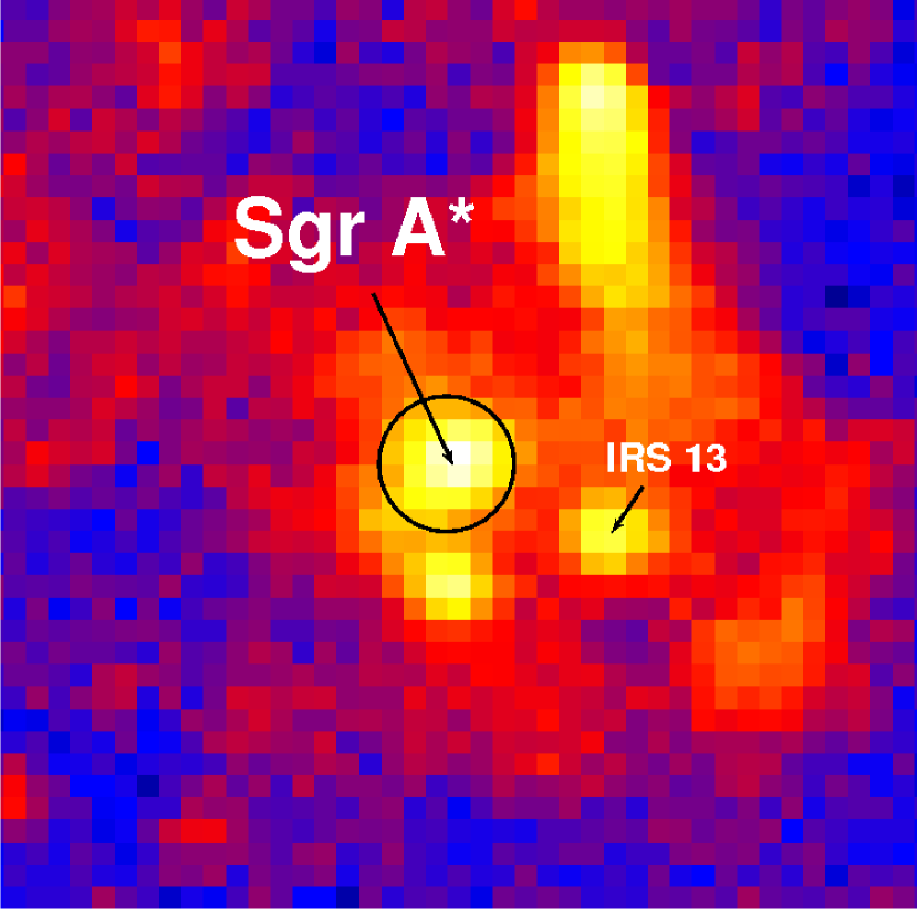
Figure 3: Chandra image (north is up and east is left) of the central $\sim 20^{\prime\prime}\times 20^{\prime\prime}$ of the Galaxy in the 2–8 keV energy band. The angular size of each pixel is $0.492^{\prime\prime}\times 0.492^{\prime\prime}$. The positions of the radiosource Sgr A* and the star cluster IRS 13 are marked. Flares of Sgr A* have been filtered out. The circle with a radius of 3 pixels drawn around Sgr A* denotes the region used for X-ray spectral analysis.

We now address the X-ray surface brightness profile of Sgr A*. Since the observations reported by B03, the Sgr A* field has been re-observed with Chandra many times. The total effective exposure accumulated is $\sim 1.2$ Ms, which represents a factor of $\sim 25$ increase with respect to B03. We used these archival data to measure the X-ray surface brightness around Sgr A*.

Since apart from the quiescent emission studied in this paper, Sgr A* also exhibits X-ray flares (Porquet et al., 2008), which likely originate in the inner regions of an accretion flow onto the SMBH (as suggested by multiwavelength and in particular radio interferometric observations, Yusef-Zadeh et al. 2009; see however our discussion in §4.2.1), we made an attempt to filter out such flares from the Chandra data. Specifically, we excluded observations in which increases by a factor of 4 or more in the X-ray flux from Sgr A* integrated over 100 s intervals were detected. The filtered data set has a total effective exposure of 620 ks. The resulting image of the central $\sim 20^{\prime\prime}\times 20^{\prime\prime}$ region of the Galaxy obtained with the ACIS-I detector is shown in Fig. 3.

Figure 4: Radial surface brightness profiles of the X-ray emission to the north and to the south of Sgr A* (open and filled circles, respectively), in comparison with the radial profile of the nearby source CXOGC J174540.9$-$290014 (crosses) normalised to match the central peak of the northern profile of Sgr A*. Also shown are the fits of the northern profile of Sgr A* and the profile of CXOGC J174540.9$-$290014 by a sum of a constant and a Gaussian with $\sigma=1.45$ and 0.75 pixels, respectively (solid lines). The Gaussian components are shown separately with the dashed lines.

Even though we display only the innermost part of the GC region in Fig. 3, the X-ray image still exhibits a lot of detail apart from the source at Sgr A*. In particular, there are two bright features within 5” of Sgr A*, including the complex IRS 13 of hot, massive stars (see Genzel, Eisenhauer, & Gillessen 2010 for a review). Both of these features are located to the south of Sgr A*. We therefore constructed two surface brightness profiles by integrating Chandra counts in one pixel-wide semi-annuli to the north and to the south of Sgr A* (Fig. 4). For comparison we show the radial profile of the presumably point-like, bright source CXOGC J174540.9$-$290014 located $\sim 20^{\prime\prime}$ from Sgr A* (and hence not shown in Fig. 3), which was also discussed by B03. This profile can be fitted (taking into account the finite width of the pixels) reasonably well by a sum of a constant and a Gaussian with $\sigma\approx 0.37^{\prime\prime}$. The latter can be used as an approximation of the point-spread function (PSF) for our mosaic Chandra image of the Sgr A* region. Fitting the northern radial profile of Sgr A* with the same model gives $\sigma\approx 0.7^{\prime\prime}$, whereas the southern profile is significantly non-Gaussian. We can therefore estimate the intrinsic (i.e. PSF subtracted) size of the central source at $\approx 0.6^{\prime\prime}$. Our estimates of the PSF width and the intrinsic size of the emission centred at Sgr A* are in good agreement with the original results of B03.

Figure 5 compares the Chandra radial profile measured to the north of Sgr A* with the X-ray surface brightness profile expected for a stellar cusp with $A=4\times 10^{6}M_{\odot}$ pc^-3, $t_{\rm{mb}}=100$ Myr and other parameter values as given in Table 1, i.e. the same model as in Fig. 2. We have converted all modelled profiles to Chandra counts using the spectral model described below in §3.4. The dotted line is the model without taking into account the angular resolution of the telescope, while the solid line shows the model convolved with a Gaussian with $\sigma=0.37$” to approximate the Chandra PSF. We see that the unconvolved model surface brightness in the innermost region is approximately inversely proportional to the projected distance (see equation 21 below). Finally, the dashed line shows the same model but assuming that the central “destruction” zone (see Fig. 2) is devoid of stars. Since complete depletion of the innermost cusp by collisions is unlikely, the solid and dashed curves may be regarded as an upper and lower limits on the expected emission, respectively.

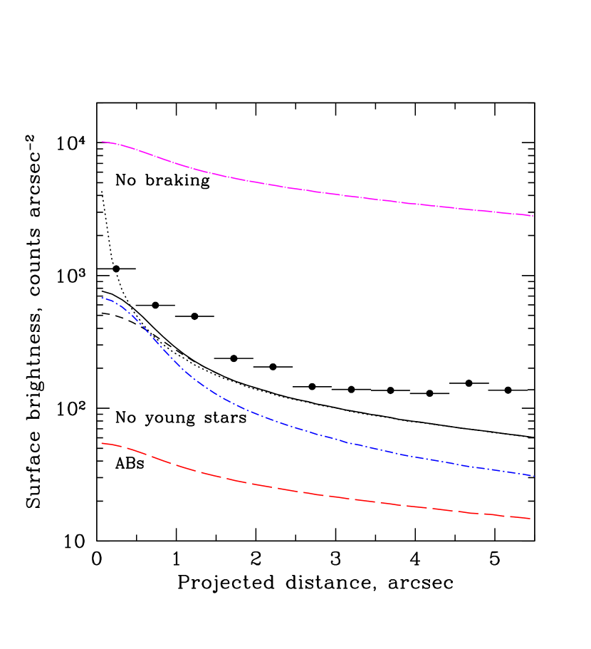
Figure 5: Surface brightness profile of the extended X-ray emission around Sgr A*. The data points are Chandra 2–8 keV measurements to the north of Sgr A*. The dotted line is a model with $A=4\times 10^{6}M_{\odot}$ pc^-3, $t_{\rm{mb}}=100$ Myr and other parameter values as given in Table 1. There is a $\sim 20$% systematic uncertainty in the normalisation of the model, associated with the conversion of the intrinsic (unabsorbed) flux to Chandra counts. The solid line is the same model convolved with a Gaussian with $\sigma=0.37$”, approximating the Chandra PSF. The short-dashed line is the model assuming that there are no stars in the central “destruction” zone (see Fig. 2). The magenta dot-long-dashed line illustrates what would be if the stars experienced no magnetic braking. The blue dot-short-dashed line is a modification of the model, in which all stars are born simultaneously 10 Gyr ago, so that there is no contribution from young (and therefore coronally active) stars. Finally, the maximal expected contribution of active binaries is shown with the red long-dashed line.

The model reproduces the innermost part of the Chandra surface brightness profile fairly well, underpredicting the measured X-ray flux from the central arcsecond by $\sim 25$%, which is comparable with the uncertainty in the conversion of the intrinsic (i.e. unabsorbed) source flux to Chandra counts (see Table 2). For comparison, we show with the magenta dot-long-dashed line in Fig. 5 the same model, but assuming that the stars experience no magnetic braking. The resulting X-ray emission is more than an order of magnitude stronger than is observed, because all stars now spin with $\Omega>0.1\Omega_{\rm{b}}$, as a result of the rotation received at birth and in tidal interactions, and produce coronal emisssion with maximal possible efficiency.

The effect of X-ray emission induced by tidal spin-ups is limited to $\sim 1.5^{\prime\prime}$ ($\sim 0.06$ pc) from Sgr A*. However, our model is also able to account for a significant fraction of the apparently diffuse X-ray emission detected by Chandra further away from Sgr A*. In our model, which assumes continuous star formation over $t_{\rm{c}}=10$ Gyr, this additional emission is partly associated with late-type MS stars that were born at most several magnetic braking times (i.e. a few $10^{8}$ yr) ago and hence continue to rotate fast and produce strong X-ray emission. Note that the region between 1” and 12” from Sgr A*, where a starburst apparently occured just $\sim 6$ Myr ago (Paumard et al., 2006), is expected to contain a large number of young, strongly X-ray emitting stellar objects that may account for a significant fraction of the apparently diffuse X-ray emission (Nayakshin & Sunyaev, 2005).

An additional significant contribution can be provided by active binaries (see the red long-dashed line line in Fig. 5) if such systems are present and have not been evaporated in the GC central cusp (see the discussion in §2.3). This combination of young stars and ABs resembles the situation in the solar neighbourhood, where young single stars, ABs and catacalysmic variables all provide similar contributions to the cumulative X-ray emission (Sazonov et al., 2006).

Importantly, the X-ray flux from the innermost $\sim 1.5^{\prime\prime}$ region is essentially determined by the total mass of late-type MS stars in the central cusp and is almost insensitive to the history of star formation preceeding the present epoch. This is illustrated in Fig. 5 with the blue dot-short-dashed line, which is the result of a computation for the same model as before but assuming that all stars were born at the same time 10 Gyr ago. The flux from the vicinity of Sgr A* is nearly the same as in the case of continuous star formation, but the emission outside $\sim 1.5^{\prime\prime}$ from Sgr A* has decreased due to the disappearance of young stars.

Figure 6: As Fig. 5, but for a set of different models. The dotted, solid and dashed lines are for $t_{\rm{mb}}=100$ Myr and $A=2$, 4 and $6\times 10^{6}M_{\odot}$ pc^-3, respectively (collisional destruction of stars in the vicinity of the SMBH is not taken into account). The dash-dotted line is for $t_{\rm{mb}}=200$ Myr and $A=3\times 10^{6}M_{\odot}$ pc^-3.

The uncertainties associated with some of our model parameters (Table 1), in particular with the mass density coefficient $A$ and magnetic braking time scale $t_{\rm{mb}}$, translate into an uncertainty of the predicted X-ray emission from stars in the vicinity of Sgr A*. In Fig. 6, we demonstrate how the X-ray surface brightness profile is modified by changing these parameters within reasonable ranges. We see that with $t_{\rm{mb}}$ fixed at 100 Myr, the data favour (if we were to explain the entire X-ray emission from Sgr A* by coronal radiation from spun-up stars) a rather high stellar density $A\sim$ (4–6)$\times 10^{6}M_{\odot}$ pc^-3 (taking into account the $\sim 20$% uncertainty in the model normalisation due to the conversion to Chandra counts). On the other hand, taking $t_{\rm{mb}}=200$ Myr, which is still a reasonable value for $\hbox{\hbox to0.0pt{\hbox{\lower 4.0pt\hbox{$\sim$}}\hss}\hbox{$<$}}M_{\odot}$ stars, we can reproduce the emission from Sgr A* already with $A\sim 3\times 10^{6}M_{\odot}$ pc^-3.

3.3 Approximate scaling formulae

Based on the results of our simulations, we can write down an approximate formula (which provides good fits to the computational results at least up to $A=1.2\times 10^{7}M_{\odot}$ pc^-3) for the expected radial profile of the intrinsic, i.e. unabsorbed, X-ray (2–10 keV) luminosity density of a stellar cusp of density $\rho_{\ast}(r)=A(r/0.25~{}{\rm pc})^{-1.3}$, assuming a magnetic braking time $t_{\rm{mb}}=100$ Myr:

$$\epsilon_{\rm{HX}}(r)\approx 7.5\times 10^{34}A_{6}^{1.6}\left(\frac{r}{0.05~{}\rm{pc}}\right)^{-2}$$

$$+3\times 10^{34}A_{6}\left(\frac{r}{0.05~{}\rm{pc}}\right)^{-1.3}~{}{\rm erg}~{}{\rm s}^{-1}~{}{\rm pc}^{-3},$$ (20)

where $A_{6}=A/(10^{6}M_{\odot}~{}{\rm pc}^{-3})$.

The first term on the right-hand side of equation (20) reflects the contribution of spun-up stars, whereas the second term is due to the combined emission of recently born (less than a few $t_{\rm{mb}}$ ago) and hence rapidly rotating stars and ABs. The latter contibution obviously scales linearly with the cusp density. In contrast, the cumulative X-ray luminosity of spun-up stars grows approximately as $A^{1.6}$ with increasing cusp density, since it is not only the total number of stars that increases, but also the relative fraction of fast rotators among them. The amplitude of the second term should be regarded as indicative only, because it can vary by a large factor depending on the actual star formation history in the cusp and the actual presence of ABs there.

Given the GC distance of 8 kpc and taking into account the absorption column $N_{\rm{H}}\approx 1.1\times 10^{23}$ cm^-2 towards Sgr A* (see Table 2 below), equation (20) translates into an approximate relation for the expected surface brightness of a GC stellar cusp in the 2–10 keV energy band:

$$S_{\rm HX,obs}(\theta)\approx 1.13\times 10^{-15}A_{6}^{1.6}\theta^{-1}$$

$$+8.6\times 10^{-16}A_{6}\theta^{-0.3}~{}{\rm erg}~{}{\rm s}^{-1}~{}{\rm cm}^{-2}~{}{\rm arcsec}^{-2},$$ (21)

where $\theta$ is the projected distance from Sgr A* in arcsec. For $A_{6}\mathrel{\hbox{\hbox to0.0pt{\hbox{\lower 4.0pt\hbox{$\sim$}}\hss}\hbox{$>$}}}2$, the first term dominates at $\theta\hbox{\hbox to0.0pt{\hbox{\lower 4.0pt\hbox{$\sim$}}\hss}\hbox{$<$}}$1–2” from Sgr A*.

It is important to emphasise that if magnetic braking, for some reason, operates less efficiently in spun-up stars in the GC region than in stars in the solar neighbourhood, i.e. $t_{\rm{mb}}>100$ Myr, then rapidly rotating stars will constitute a larger fraction of all stars in the cusp and thus produce more X-ray emission per unit stellar mass, e.g. by $\sim 50$% if $t_{\rm{mb}}=200$ Myr for a given value of $A$. A similar effect may result if the X-ray luminosity of the stellar cusp is dominated by (presumably) much more numerous K/M dwarfs rather than by Sun-like stars. In either case, it is possible that a somewhat lighter stellar cluster, than predicted by equation (21), could produce a given X-ray flux from Sgr A*.

3.4 X-ray spectrum

We have demonstrated that a high-density cusp of late-type MS stars in the GC region can produce X-ray emission with the radial surface brightness profile as observed by Chandra near Sgr A*. Will this emission from rapidly spinning stars also have a spectrum similar to that of Sgr A*?

To answer this question, we re-measured the spectrum of Sgr A* reported by B03. Since the GC region is rich in high-energy phenomena, a significant or even dominant fraction of the X-ray emission observed outside of the innermost few arcseconds (see the image in Fig. 3) may have a different nature from the central X-ray cusp. We therefore constructed a spectrum from the photons detected within 3 pixels ($\approx 1.5^{\prime\prime}$) of Sgr A*. We modelled the detector background for Chandra/ACIS using the $acisbg$ task (http://cxc.cfa.harvard.edu/contrib/maxim/acisbg/) based on the stowed dataset. The background-subtracted 2–8 keV flux from the studied region is $1.45\times 10^{-13}$ erg s^-1 cm^-1 (with a statistical uncertainty of a few per cent), in good agreement with B03.

In agreement with B03, the measured spectrum of Sgr A* (Fig. 7) is consistent with thermal emission of optically thin, hot plasma, modified at low energies by absorption in cold gas. In addition, we detect a $\sim 3\sigma$ significant excess that is consisent with a 6.4 keV fluorescent line of neutral iron. We fitted the Chandra data in the 2–8 keV energy band by different models in XSPEC (version 12.5.1, Arnaud 1996) and found that a good fit is provided by the model $wabs*(cevmkl+gauss)$. The best-fit parameters are given in Table 2 and the spectral fit is shown in Fig. 7. CEVMKL is a sum of MEKAL (Mewe, Gronenschild, & van den Oord, 1985; Liedahl, Osterheld, & Goldstein, 1995) models for optically thin plasmas with a range of temperatures and a power-law distribution of emission measures, $d{\rm EM}\propto(T/T_{\rm max})^{\alpha-1}dT/T_{\rm max}$, where we fix $\alpha=1$ (the results are only weakly sensitive to this parameter). In fact, using a single-temperature MEKAL model instead of CEVMKL provides a similarly good fit to the strongly absorbed spectrum of Sgr A*, but we have chosen CEVMKL because it is more physically justified in application to X-ray spectra of coronally active stars.

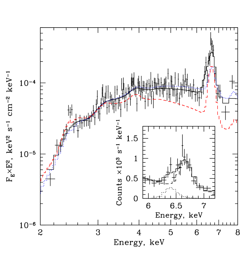
Figure 7: Spectrum of X-ray emission from the region with radius of 1.5” around Sgr A* measured by Chandra in the 2–8 keV energy band (data points) and its best fit by the $wabs*(cevmkl+gauss)$ model with the parameters given in Table 2. For comparison shown are the best-fit $cevmkl$ models (see Table 2) of ASCA spectra of the coronally active stars V711 Tau (blue dotted) and 47 Cas B (red dashed), modified by cold gas absorption with $N_{\rm{H}}=1.08\times 10^{23}$ cm^-2 and normalised to match the spectral flux of Sgr A* at 3 keV. The inset shows a blow-up of the Sgr A* spectrum at $\sim$6–7 keV. The 6.4 keV line and CEVMKL components are shown by the dotted and dashed lines, respectively.

Table 2: Best-fit spectral parameters for the X-ray emission within 1.5” of Sgr A* and for two coronally active stars.

Parameter	Sgr A*	V711 Tau	47 Cas B
	Chandra/ACIS-I (2–8 keV)	ASCA/GIS (2–9 keV)
	$wabs*(cevmkl+gauss)$	$cevmkl$
$T_{\rm max}$ (keV)	$3.2\pm 0.3$	$3.74\pm 0.08$	$2.4\pm 0.3$
$\alpha$	1 (fixed)	1 (fixed)	1 (fixed)
$A_{\rm Fe}$	$0.80\pm 0.12$	$0.32\pm 0.07$	1 (fixed)
$N_{\rm{H}}$, cm-2	$(10.8\pm 0.6)\times 10^{22}$	—	—
${\rm EW}_{6.4~{}{\rm keV}}$ (eV)	$110_{-40}^{+30}$	—	—
$\chi^{2}$/dof	156/130	419/315	33/49
Unabsorbed 2–10 keV flux (erg s-1 cm-2)	$(4.3\pm 0.8)\times 10^{-13}$	$2.9\times 10^{-11}$	$2.4\times 10^{-12}$
Distance (pc)	$8\times 10^{3}$	29.0	33.6
Unabsorbed 2–10 keV luminosity (erg s-1)	$(3.3\pm 0.6)\times 10^{33}$	$2.9\times 10^{30}$	$3.2\times 10^{29}$

Notes: The abundances of all elements except Fe were fixed at solar values (Grevesse & Sauval, 1998). The derived Fe abundance for V711 Tau is indicative only, given the simplicity of the adopted model. The quoted distances to the stars are based on Hipparcos parallax measurements (Perryman & ESA, 1997).

Table 2 also gives the absorption-corrected flux and luminosity of Sgr A* in the 2–10 keV band for the adopted spectral model. These values have $\sim 20$% uncertainties. In summary, all of the characteristics of the X-ray spectrum of Sgr A* derived here are in good agreement with the estimates of B03 (although these authors used a single-temperature thermal model), but the associated statistical uncertainties have now become small due to the greatly increased observational time and statistics.

3.4.1 Comparison with stellar spectra

According to the reference mass density model (equation 1, $A=4\times 10^{6}M_{\odot}$ pc^-3), which we used to describe the X-ray surface brightness profile (Fig. 5), the total mass of stars and stellar remnants within the cylinder with a projected radius of 1.5” around Sgr A* is $8.4\times 10^{4}M_{\odot}$ ($6.3\times 10^{4}M_{\odot}$) within $\pm 0.25$ pc ($\pm 0.1$ pc) along the line of sight. Since within $\sim 0.1$ pc from Sgr A* the bulk of the coronal X-ray luminosity is produced by $\sim 10$% of low-mass stars (see the bottom panel of Fig. 2 and the related discussion in §3) and we assumed $f_{\rm{LMS}}=0.5$, the X-ray flux accumulated by Chandra within 1.5” of Sgr A* can be produced by some 3–5 thousand rapidly spinning stars, each emitting $10^{29}$–$10^{30}$ erg s^-1 in the 2–10 keV energy band.

As was mentioned in §2.2.3, there is a well-known trend of X-ray spectral hardening with increasing coronal luminosity, which in turn is closely linked to stellar rotation. Although the rotational velocities are expected to vary from one star to another in a GC stellar cusp, its cumulative X-ray emission will be dominated by stars that are in ($\Omega>\Omega_{\rm{c}}$) or close to being in ($\Omega\hbox{\hbox to0.0pt{\hbox{\lower 4.0pt\hbox{$\sim$}}\hss}\hbox{$<$}}\Omega_{\rm{c}}$) saturation regime of coronal activity (see again the bottom panel of Fig. 2).

An ultimate spectral test of our model would consist in constucting a composite X-ray spectrum of an ensemble of stars rotating at various angular velocities representing the distribution of $\Omega$ values predicted by the model. We feel that performing such a computation is premature given the relative simplicity of our current model. In particular, this model deals with only one type of star, namely $1M_{\odot}$ dwarfs. In reality, depending on the composition of the GC stellar cusp, its X-ray luminosity may be dominated by K/M dwarfs rather than by less numerous Sun-like stars. The rotational velocity distributions and X-ray spectra may be somewhat different for stars of different types, and a composite spectrum of the stellar cusp should take this into account. Perhaps more importantly, the combined spectrum of the stellar cusp may contain a significant contribution from giant stellar flares (with $L_{\rm{X}}\sim L_{\rm{bol}}$), especially at energies above $\sim 3$ keV. As discussed in §4.2.1 below, the statistics of such flares remains very limited. Moreover, such events are usually detected by all-sky monitors and their X-ray spectra are poorly studied at brightness peak. This renders it practically impossible to estimate the contribution of giant flares to the cumulative X-ray spectrum of the stellar cusp. In view of these complications and uncertainties, we restrict our discussion below to a fairly qualitative comparison of the spectrum of the extended emission from Sgr A* with the spectra of a couple of well-studied coronally active stars in the Solar neighbourhood.

The first object, V711 Tau, is a well-known RS CVn system. It consists of K0-2 IV and G0-5 V stars, tidally locked with a period of 2.84 days (Fekel, 1983). Given the masses and radii of the components of $M_{1}=1.4\pm 0.2M_{\odot}$, $M_{2}=1.1\pm 0.2M_{\odot}$, $R_{1}=3.9\pm 0.2R_{\odot}$ and $R_{2}=1.3\pm 0.2R_{\odot}$ (Fekel, 1983), the subgiant component rotates at a significant fraction of its breakup velocity, $\Omega/\Omega_{\rm{b}}\approx 0.27$, and is therefore definitely in saturated regime of coronal activity. We emphasise that although V711 Tau is an active binary, its spectral properties should resemble those of a single star that has just been spun up by a strong tidal interaction to $\Omega>\Omega_{\rm{c}}$.

The other object, 47 Cas B, is a relatively young ($\sim 100$ Myr old) solar analog (spectral type G0-2 V) belonging to the Pleiades moving group (Telleschi et al., 2005). It has a likely rotation period of $\sim 1$ day (see Telleschi et al. 2005 and references therein), so that $\Omega/\Omega_{\rm{b}}\sim 0.1$, with this fast rotation being due to the star’s young age rather than due to its binarity (the star is actually a member of a wide binary system). It might thus be close to but not necessarily fully in saturation regime of coronal activity. Therefore, 47 Cas B probably more closely resembles a typical spun-up star in the GC stellar cusp than V711 Tau.

We obtained the X-ray spectra of these two systems using archival data of the GIS instrument aboard the ASCA observatory. Both spectra are well fit in the 2–9 keV band by the CEVMKL model. The best-fit parameters are given in Table 2. The fit for V711 Tau could be improved further by allowing the abundances of S, Si and other metals to vary, but such small modifications are unimportant for our current purpose of comparing the spectral continua of Sgr A* and coronally active stars. Fig. 7 shows the best-fit models for V711 Tau and 47 Cas B, modified by cold gas absorption with $N_{\rm{H}}=1.08\times 10^{23}$ cm^-2, as measured for Sgr A*, and normalised to the flux of Sgr A* at 3 keV.

We see that the spectra of V711 Tau and 47 Cas B are slightly harder and somewhat softer, respectively, than the spectrum of Sgr A*. This appears to be consistent with i) V711 Tau having saturated coronal activity – as witnessed by its very high hard X-ray luminosity, $L_{\rm{HX}}\sim 3\times 10^{30}$ erg s^-1 (2–10 keV, Table 2) and ii) 47 Cas B being not quite saturated – its X-ray luminosity of $\sim 2.5\times 10^{30}$ erg s^-1 (0.1–10 keV, Telleschi et al. 2005, of which $\sim 3\times 10^{29}$ erg s^-1 is at 2–10 keV, Table 2) might be somewhat below the saturation level of $\sim 10^{-3}L_{\rm{bol}}$.

Although it is difficult to draw firm conclusions from this exemplary analysis, it indicates that the non-flaring emission of an ensemble of spun-up stars can produce a spectrum that is sufficiently hard to explain the low-energy (below $\sim 4$ keV) spectral continuum observed from Sgr A*. However, to account for the hard X-ray (at energies above $\sim 4$ keV) flux from Sgr A* within the stellar cusp model, one possibly needs an additional significant contribution from giant stellar flares. This appears plausible (see §4.2.1 and §4.2.2) but requires further study.

3.4.2 Iron abundance

The Chandra spectrum of Sgr A*, in particular the strength of the 6.7-7.0 keV blend of FeXXV and FeXXVI lines, indicates a somewhat sub-solar ($\sim 0.7$–0.9 relative to the solar value of Grevesse & Sauval 1998) abundance of iron in the X-ray emitting plasma. This result appears to be consistent with the model of cumulative emission of coronally active stars.

Indeed, both V711 Tau and 47 Cas B exhibit significantly subsolar iron abundances. For V711 Tau, this is already suggested by the ASCA spectrum presented here: $A_{\rm Fe}\sim 0.3$. More reliable estimates are provided by analyses of high-resolution spectra obtained with the Reflection Grating Spectrometer on XMM-Newton, which indicate $A_{\rm Fe}\sim 0.2$ (Audard et al., 2003) and $\sim 0.5$ (Telleschi et al., 2005) for V711 Tau and 47 Cas B, respectively (for the Fe abundance of Grevesse & Sauval 1998). These examples reflect the well-known phenomenon of reduced abundance of iron and other low first ionisation potential elements in active stellar coronae (see Güdel 2004 for a review).

3.4.3 6.4 keV emission

Combined radiation of coronally active stars can also possibly account for at least part of the flux of 6.4 keV emission apparent in the Chandra spectrum of Sgr A* (see Fig. 7). Indeed, a significant fraction (up to 50%) of the hard X-ray emission produced in the corona of a star irradiates the underlying chromosphere and photosphere and produces fluorescent emission, mainly in the 6.4 keV line of iron. Such fluorescent emission provides a means of probing the geometry of coronal flares and the photospheric abundance of iron.

This problem has been of interest for a long time in application to the Sun, first theoretically (Bai, 1979; Basko, 1979) and then observationally as powerful 6.4 keV emission was actually observed during solar flares (e.g. Culhane et al. 1981; Phillips et al. 1994). Recently, 6.4 keV emission has also been detected during coronal flares of few other stars, including the RS CVn binary II Peg (Osten et al., 2007), the G-type giant HR 9024 (Testa et al., 2008) and the M dwarf EV Lac (Osten et al., 2010). The measured equivalent widths of the 6.4 keV line range from a few tens to $\sim 200$ eV, which is similar to the values reported for solar flares and agrees with the expected flux of fluorescent emission arising due to irradiation of a stellar atmosphere of solar Fe abundance by hard X rays from a coronal loop located at $\hbox{\hbox to0.0pt{\hbox{\lower 4.0pt\hbox{$\sim$}}\hss}\hbox{$<$}}0.3R_{\ast}$ above the atmosphere (Drake, Ercolano, & Swartz, 2008).

To our knowledge, there have been no reports of 6.4 keV emission in non-flaring spectra of coronally active stars, probably due to the insufficient sensitivity and/or low spectral resolution of the existing instruments and the presence of the much stronger 6.7 keV and 7.0 keV line complexes of iron in coronal spectra. However, based on the existing evidence for solar and stellar flares we may expect the integrated spectrum of a cusp of rapidly spinning stars to contain a 6.4 keV line with an equivalent width ${\rm EW}\sim 50$ eV. Moreover, as is further discussed below in §4.2.2, if giant coronal flares contribute significantly to the cumulative X-ray emission of the cusp, somewhat stronger fluorescent emission can be expected, possibly consistent with the value ${\rm EW}=110^{+30}_{-40}$ eV measured in the spectrum of Sgr A*.

Another possibility to explain part of the observed 6.4 keV emission is fluorescent emission from a cold gas permeating the stellar cusp. However, in order to account for, say, ${\rm EW}\sim 50$ eV, this gas must have a column density $\sim 3\times 10^{23}$ cm^-2, assuming irradiation by $\sim 3.2$ keV thermal emission from Sgr A*, solar abundance of iron (${\rm Fe}/{\rm H}=3.16\times 10^{-5}$) and adopting the ionisation cross sections from Verner & Yakovlev (1995) and fluorescent yield of 0.34. This is much larger than the total absorption column of $\approx 10^{23}$ cm^-2 measured by Chandra towards Sgr A*.

We conclude that photospheric fluorescent emission accompanying the coronal activity of spun-up stars can possibly explain the tentatively detected 6.4 keV emission from Sgr A*.

4 Discussion

We have demonstrated that the combined coronal radiation of a high-density cluster of late-type MS stars “rejuvenated” by tidal interactions can in principle explain the main properties of the quiescent X-ray emission from Sgr A*, namely its characteristic size (${\rm FWHM}\sim 1.5^{\prime\prime}$), luminosity ($\sim 10^{33}$ erg s^-1, observed in the 2–10 keV band) and possibly (this issue needs further study) spectrum (optically thin thermal emission with $kT\hbox{\hbox to0.0pt{\hbox{\lower 4.0pt\hbox{$\sim$}}\hss}\hbox{$<$}}3.5$ keV, absorbed by $N_{\rm{H}}\sim 10^{23}$ cm^-2). In this scenario, extended X-ray emission is produced by several thousand rapidly spinning stars (with periods of $\mathrel{\hbox{\hbox to0.0pt{\hbox{\lower 4.0pt\hbox{$\sim$}}\hss}\hbox{$>$}}}1$ day) with nearly saturated coronal activity.

Below, we first discuss the implications of our model for the mass density of the GC stellar cusp (§4.1), then compare the observational properties of the model with those of truly diffuse X-ray emission from a hot accretion flow onto the SMBH (§4.2) and finally discuss the implications for the accretion onto the SMBH (§4.3).

4.1 Implications for the GC stellar cusp

The existence of a cusp in the number density distribution of low-mass MS stars near Sgr A* has not yet been proven by direct observations. According to our baseline model, to explain the bulk of the X-ray emission from Sgr A* there must be $\sim$ (2–3)$\times 10^{4}$ Sun-like stars within a column of 1” radius centered on Sgr A* (within 0.25 pc along the line of sight). This number corresponds to a range $\sim$ (4–6)$\times 10^{6}M_{\odot}$ pc^-3 for the coefficient $A$ characterising the radial profile of stellar mass density (equation 1) and to a relative fraction $f_{\rm{LMS}}=0.5$ of low-mass stars per $M_{\odot}$.

Equations (20) and (21) can be used to predict the contribution of coronal radiation of low-mass stars (not only spun-up stars but also young stars and active binaries) to the observed X-ray emission from the Sgr A* region for a given density of the GC stellar cusp, assuming that tidally spun-up stars experience efficient magnetic braking ($t_{\rm{mb}}=100$ Myr).

As follows from our discussion in §2.1, the space density of stars required to explain the quiescent X-ray flux from Sgr A* somewhat exceeds the range $A\sim$ (1–3) $\times 10^{6}M_{\odot}$ pc^-3, suggested by the available statistics of bright stars in the central parsec of the Galaxy. Furthermore, it is possible that low-mass stars near Sgr A* are underabundant near Sgr A*, as suggested by the paucity of red giants in the central several arcseconds. However, the number of low-mass stars in the central arcsecond required to explain the Chandra data is consistent with the upper limit deduced from the measured surface brightness of NIR diffuse light near Sgr A* (see equations 3 and 4).

Furthermore, it is possible that a cusp of low-mass stars will produce a higher X-ray luminosity for a given density than implied by our baseline model:

1. First, if magnetic braking operates somewhat less efficiently than assumed, then a larger fraction of the stars will retain their fast rotation since their last spin-up episode. As we discussed in §3.3, increasing the characteristic time $t_{\rm{mb}}$ from 100 Myr to a still reasonable (especially for K/M dwarfs) 200 Myr leads to a 50% increase in the luminosity of the stellar cusp.

2. Secondly, as discussed in §4.2.1 below, multiple giant stellar flares may significantly increase the X-ray luminosity of the stellar cusp.

3. Thirdly, in our baseline model stellar remnants played a relatively unimportant role, as we assumed their relative fraction to be $f_{\rm{SR}}=0.25$ and the average mass $M_{\rm{SR}}=1M_{\odot}$. In reality, the innermost region of the Galaxy may be overpopulated by stellar-mass black holes (e.g. Morris 1993; Freitag, Amaro-Seoane, & Kalogera 2006; Löckmann, Baumgardt, & Kroupa 2010). These heavy objects can spin up low-mass stars much more efficiently than stars or white dwarfs (see AK01).

4. Finally, in our simulations we implicitly assumed that stars were in circular orbits around the SMBH. A more accurate computation should take into account mutual interactions of stars moving in eccentric orbits around the SMBH, which might increase the number of spun-up stars.

In summary, given the remaining uncertainties on the observational side and the fact that the presented model is somewhat simplistic, it seems plausible that a factor of few less stars in the central region might still produce the bulk of the X-ray flux observed from Sgr A*.

4.2 Comparison with accretion flow models

The crucial question is how to distinguish observationally the combined coronal radiation of a cluster of spun-up stars from the diffuse emission of a quasi-spherical accretion flow of hot gas onto the central SMBH, which has been the favoured explanation for the quiescent X-ray emission from Sgr A* so far. Below, we discuss differences and similarities between the two models.

4.2.1 Variability and flares

We have so far assumed that the X-ray luminosity emitted by a coronally active star is solely determined by its current rotation rate. In reality, virtually all stars with coronae experience flares during which their X-ray luminosity increases by orders of magnitude. Therefore, the cumulative X-ray emission of a GC stellar cusp must be variable at some level.

Statistics of coronal flares in stars of different types implies (see §13 in the review of Güdel 2004 and references therein) that X-ray/UV flare luminosities (or total energies) obey a power law with a slope of $\approx 2$, i.e. $dN/dL\propto L^{-2}$, and it remains unclear if the strongest or weakest flares dominate in the long term-integrated energy output of stellar coronae and if the ”quiescent” luminosity is in fact just a superposition of weak flares.

Particularly interesting are giant flares observed from nearby RS CVn systems. Only a few dozen such flares have been detected in several decades of X-ray astronomical observations by all-sky monitors (see Arefiev, Priedhorsky, & Borozdin 2003). In particular, the SSI instrument aboard the Ariel V spacecraft detected 7 flares that were attributed to RS CVn binaries (Pye & McHardy, 1983), including 2 flares from one of the best studied systems II Peg. Interestingly, all these flares had similar properties, namely peak luminosities of (1–6)$\times 10^{32}$ erg s^-1 (in the 2–18 keV energy band), characteristic durations $\sim 5$ hours and total emitted energies (in the X-ray band) $\sim 6\times 10^{36}$ erg s^-1. Based on this statistics, Pye & McHardy (1983) concluded that a typical RS CVn binary produces about 1 such giant flare per year. This explains why dedicated observations of individual RS CVn systems by X-ray telescopes, which typically last less than a day, fail to detect such extreme flares.

On Dec. 16, 2005, another giant flare was detected from II Peg by the hard X-ray instrument BAT and X-ray telescope (XRT) aboard the Swift spacecraft (Osten et al., 2007). These observations provided uniquely detailed, broad-band information on a giant flare. During the flare, the luminosity peaked at $\sim 1.3\times 10^{33}$ and $\sim 8\times 10^{32}$ erg s^-1 in the 0.8–10 keV and 10–200 keV, respectively. Thus, the total X-ray luminosity of the corona for 1–2 hours reached $\mathrel{\hbox{\hbox to0.0pt{\hbox{\lower 4.0pt\hbox{$\sim$}}\hss}\hbox{$>$}}}40$% of the bolometric luminosity of the binary system ($\sim 5\times 10^{33}$ erg s^-1, Mewe et al. 1997). For comparison, the non-flaring X-ray (0.5–12 keV) luminosity of II Peg is $\sim 10^{31}$ erg s^-1 (Huenemoerder, Canizares, & Schulz, 2001), or $\sim 10^{-3}$ of its bolometric luminosity. This implies that stellar coronae that are already in a saturation regime can brighten up by an additional factor of $\mathrel{\hbox{\hbox to0.0pt{\hbox{\lower 4.0pt\hbox{$\sim$}}\hss}\hbox{$>$}}}100$ during giant flares.

New data on giant flares are now coming from the MAXI all-sky monitor on the International Space Station. Already during the first year of operation it detected 14 flares from 7 RS CVn binaries, including 2 huge flares with peak (1.5–10 keV) luminosities $\sim 5\times 10^{33}$ erg s^-1 from II Peg and GT Mus (Tsuboi et al., 2011). These new results, first, confirm that giant flares occur roughly once a year per RS CVn system and, second, suggest that stellar coronae may produce even more extreme flares than was considered possible before.

The spun-up stars in a GC cusp should be similar to RS CVn systems as regards their coronal activity, apart from being less luminous by a factor of few, since the X-ray bright component in RS CVn binaries is often a subgiant rather than a normal star. We may thus expect every spun-up star to undergo a giant X-ray flare with a luminosity of $10^{32}$–$10^{33}$ erg s^-1 and duration of a few hours roughly once a year. A ”superflare” of the M dwarf EV Lac (Osten et al., 2010), already mentioned in §3.4.3, at the peak of which the X-ray (0.3–100 keV) luminosity reached more than 3 bolometric luminosities of the star, might serve as a good example of such a giant flare on a single coronally active star (note, however, that this particular flare was fairly short, $\sim 0.5$ hour).

Given that some 3–5 thousand spun-up stars are required to produce the measured X-ray flux from Sgr A*, we may expect several stars to experience giant flares at any moment. The cumulative luminosity of these flares may be comparable or exceed the total luminosity of the remaining several thousand ”quiescent” stars. In fact, due to flaring activity the integrated X-ray luminosity of a GC stellar cusp can be significantly higher than expected based on equations (18) and (19).

If the cumulative emission of spun-up stars is dominated by strong flares, we can expect the X-ray flux from Sgr A* to vary on hourly and daily time scales by tens of per cent or even by a factor of few, due to the changing number and intensity of flares. This variability should be especially strong at higher energies, i.e. around 10 keV and above, because the coronal emission spectrum hardens during flares, as for example was the case during the superflare of II Peg (Osten et al., 2007). In principle, the already existing Chandra and XMM-Newton data can be used to verify this prediction. Furthermore, it is possible that some of the weaker, $\sim 1$ hour long X-ray flares observed from Sgr A* (e.g., Baganoff et al. 2003; Porquet et al. 2008) were in fact produced by stellar coronae.

At the same time, it is clear that the stronger X-ray flares observed from Sgr A*, during which its luminosity reaches several $\times 10^{34}$ and even more than $10^{35}$ erg s^-1, are of different origin and most likely produced in the close vicinity of the SMBH (see Genzel, Eisenhauer, & Gillessen 2010 for review). In particular, by analysing the Chandra data for some of such flares we have verified that their origin is consistent with a point source (within the Chandra PSF) at the position of Sgr A*.

4.2.2 Multifrequency properties

The primary radiative component of active stellar coronae is optically thin X-ray emission of a multitemperature gas, with a dominant temperature $kT\sim$ a few keV. A similar X-ray spectrum can be produced by a hot accretion flow if the accretion rate is sufficiently low. In this case, the bulk of the total X-ray luminosity is due to gas near the Bondi radius $R_{\rm{B}}\sim 0.05$ pc, whereas the additional emission produced in the inner regions of the presumably advection-dominated accretion flow is relatively unimportant. As argued by Quataert (2002), such a situation may be realised in the quiescent state of the SMBH associated with Sgr A*, for which $L_{\rm{HX}}\sim 10^{-11}L_{\rm{Edd}}$, where $L_{\rm{HX}}$ and $L_{\rm{Edd}}$ are the observed X-ray luminosity and the SMBH Eddington luminosity, respectively.

Given the same thermal character of the X-ray emission in the scenarios of a cluster of spun-up stars and hot accretion flow onto the SMBH, are there spectral features that could distinguish these models from one another?

Thermal X-ray lines

Both models naturally produce coronal X-ray lines, in particular a 6.7 keV line of FeXXV. As we showed in §3.4.2, the Chandra spectrum in the 6.7 keV region indicates a somewhat subsolar abundance of Fe for Sgr A*, which is in line with the known trend for active stellar coronae. However, the measured deviation from the solar abundance is minor ($A_{\rm Fe}\approx 0.7$–0.9) and does not seem to contradict the hot accretion flow model for Sgr A* either. Indeed, recent studies of chemical abundances in the atmospheres of supergiants belonging to young stellar clusters near Sgr A* have demonstrated that these several million-old stars were formed from an interstellar medium with a nearly solar Fe/H ratio (see Davies et al. 2009 and references therein). Therefore, one can expect the gas currently feeding the SMBH to have approximately solar Fe abundance as well.

What could the widths of the X-ray lines tell us? In the stellar cusp model, the line widths should reflect the emission-weighted, radially integrated distribution of projected stellar velocities. Given equation (6) and the model surface brightness profile shown in Fig. 5, the lines produced within $\sim 1^{\prime\prime}$ of Sgr A* should be broadened by $\sigma\sim 500$ km s^-1, which corresponds to ${\rm FWHM}\sim 25$–30 eV for the 6.7 line of iron. Hence, the lines are unresolvable with CCD detectors.

It is more difficult to predict the line widths in the case of a hot accretion flow onto the SMBH. In ADAF-type models, ions tend to acquire the virial velocities in the gravitational potential of the black hole (Narayan & Yi, 1994). However, in the case of Sgr A* most of the luminosity measured by Chandra from the central arcsecond is believed to be produced near the Bondi radius. In this case, the broadening of the lines of heavy elements is probably determined by bulk motions in the gas, which should be of the order of the stellar velocity dispersion if the gas is supplied by winds of hot stars (see, e.g., Quataert 2004; Cuadra et al. 2006).

Therefore, to a first approximation, thermal X-ray lines should be similarly broadened in both scenarios.

6.4 keV line

A stand-alone issue is 6.4 keV emission of neutral (or weakly ionised) iron. As we discussed in §3.4.3, we have tentatively detected such a line, with an equivalent width ${\rm EW}=110_{-40}^{+30}$ eV in the Chandra spectrum.

There is no obvious reason to expect 6.4 keV emission in the scenario of a hot accretion flow onto the SMBH. On the contrary, as we discussed in §3.4.3, a 6.4 keV line is naturally produced in stellar coronae, due to the irradiation of the underlying photosphere by the coronal radiation and subsequent fluorscence. We noted, however, that ”quiescent” coronae are unlikely to produce 6.4 keV emission stronger than ${\rm EW}\sim 50$ eV. However, during strong flares, the coronal spectrum becomes significantly harder (see below), hence a larger fraction of the total luminosity is emitted above the ionisation thereshold of iron (7.1 keV) and consequently a 6.4 keV line with a larger equivalent width can be produced. For example, during a “superflare” from the M dwarf EV Lac, 6.4 keV emission with ${\rm EW}\sim 200$ eV was detected by Swift/XRT (Osten et al., 2010).

Therefore, if strong flares significantly contribute to the X-ray luminosity of the stellar cusp, we may expect a strong 6.4 keV line with ${\rm EW}\hbox{\hbox to0.0pt{\hbox{\lower 4.0pt\hbox{$\sim$}}\hss}\hbox{$<$}}100$ eV to be present in the X-ray spectrum. This feature, if confirmed with higher statistical significance by future observations (in particular, by long observations with the Chandra High Energy Tranmission Grating, HETG), is thus a clear indicator in favour of the stellar cusp model for the extended X-ray emission from Sgr A*.

Hard X-ray emission

If the X-ray source at Sgr A* is associated with a Bondi/ADAF accretion flow onto the SMBH, then in addition to the dominant soft X-ray emission originating in the vicinity of the Bondi radius there should be a hard X-ray continuum due to the bremsstrahlung emission from the much hotter accretion flow at $R\ll R_{\rm{B}}$, whose luminosity (at energies above 10 keV) might be $\sim 1/3$ of the X-ray luminosity (below 10 keV) of Sgr A* (Quataert, 2002). Non-thermal (e.g. synchrotron or syncrotron-self-Compton) emission produced in the innermost region of the accretion flow may provide some additional hard X-ray flux. Therefore, a hard X-ray continuum is a generic feature of Bondi/ADAF models for Sgr A*.

A significant hard X-ray continuum is also expected in the case of a cluster of spun-up, coronally active stars. Indeed, as we have already discussed, strong coronal flares can contribute significantly to the total X-ray luminosity of the GC cusp. It is well-known (see e.g. Dennis & Schwartz 1989; Aschwanden 2002 for reviews) that in solar flares only part of the total energy released via magnetic reconnection goes into heating of thermal plasma, and only a fraction of this thermal energy is radiated away as X-ray (and UV) emission. A significant amount of energy goes into acceleration of non-thermal electrons and ions. The non-thermal electrons lose a small fraction of their energy as hard X-ray bremsstrahlung and radio gyrosynchrotron emission.

During solar flares, non-thermal hard X-ray emission is some 5 orders of magnitude weaker than thermal X-ray emission (see Fig. 94 in Aschwanden 2002). However, during the 2005 giant flare of the RS CVn binary II Peg, its hard X-ray and soft X-ray luminosities were comparable (see S4.2.1 above). Therefore, if strong flares play a significant role in the combined emission of the GC stellar cusp, it might emit in total $\hbox{\hbox to0.0pt{\hbox{\lower 4.0pt\hbox{$\sim$}}\hss}\hbox{$<$}}10^{33}$ erg s^-1 in hard X-rays (at energies above 10 keV), corresponding to a hard X-ray flux $\hbox{\hbox to0.0pt{\hbox{\lower 4.0pt\hbox{$\sim$}}\hss}\hbox{$<$}}10^{-13}$ erg s^-1 cm^-2 for the GC distance of $\approx 8$ kpc. Such a signal can in principle be detected by the NuSTAR telescope, to be launched in 2012, which will have $\sim 10^{\prime\prime}$ (FWHM) angular resolution and reach sensitivity $\sim 10^{-14}$ erg s^-1 cm^-2 in the 10–30 keV energy band for an exposure of 1 Ms (Harrison et al., 2010). As we discussed in §4.2.1 above, this hard X-ray signal should be significantly variable on time scales of hours and days as a result of flaring activity on stars.

We conclude that both the stellar cusp and the accretion flow models predict hard X-ray bremsstrahlung emission at some significant level, although these predictions are very uncertain at the moment.

Gamma-ray emission

Besides electrons, also protons and ions are accelerated in coronal flares, reaching kinetic energies up to GEVs. In the case of the Sun, just a small fraction of such sub-cosmic rays escape into interplanetary space, while the majority eventually hit the lower corona and chromosphere and lose energy there (see Dennis & Schwartz 1989; Aschwanden 2002 for reviews). A small fraction of the energy lost by these particles (and also by high-energy electrons) is emitted as gamma-ray continuum and gamma-ray lines.

Similarly to the case of hard X-ray emission, it is difficult to predict the gamma-ray luminosity of a cluster of spun-up stars. In solar flares, comparable amounts of energy are emitted in the hard X-ray and gamma-ray bands, which reflects the more fundamental fact that similar amounts of energy are injected into acceleration of electrons and ions (see §7 and in particular Figs. 86 and 94 in Aschwanden 2002). Therefore, following our suggestion that a GC stellar cusp may produce up to $\sim 10^{33}$ erg s^-1 in hard X rays, it is possible that a similar luminosity is also emitted in gamma-rays, mainly at 0.5–10 MeV.

This predicted flux of gamma quanta, $\hbox{\hbox to0.0pt{\hbox{\lower 4.0pt\hbox{$\sim$}}\hss}\hbox{$<$}}10^{-7}({\rm MeV}/E)$ s^-1 cm^-2 (where $E$ is the photon energy), is too weak to be detected by present-day gamma-ray telescopes. For example, the SPI spectrometer aboard the INTEGRAL observatory, after observing the Galactic bulge region for more than 10 Ms, detects 511 keV positron-annihilation emission with a flux $\sim 10^{-3}$ s^-1 cm^-2 and provides upper limits $\sim 10^{-4}$ s^-1 cm^-2 on gamma-ray emission in the 0.511–10 MeV energy range (Churazov et al., 2011). Moreover, the angular resolution of the existing gamma-ray instruments is by far insufficient to study the Sgr A* region. Therefore, detection of gamma-ray emission from a GC stellar cusp may be a matter of distant future.

As concerns the scenario of a hot accretion flow onto the SMBH, Mahadevan, Narayan, & Krolik (1997) attempted to predict the gamma-ray luminosity of Sgr A* in the ADAF context. Some of their models resulted in a strong flux $\sim 10^{-7}$ s^-1 cm^-2 of $\sim 100$ MeV photons due to the decay of neutral pions, with a much weaker emission being produced at both lower and higher energies. However, we feel that these estimates should be regarded as indicative at best due to the many assumptions involved.

Radio emission

Related to the production of hard X rays and gamma-rays is the question of radio emission. The radio emission of stellar coronae has been well studied, so we can make relatively robust estimates in this case. It has been shown (Guedel & Benz, 1993) that across several decades in luminosity there is a linear correlation between the soft X-ray and radio (6 or 3.6 cm) luminosities, $L_{\rm{X}}/L_{\rm R}\sim 10^{5.5}$, the same for different classes of stars. Moreover, roughly the same relation seems to hold for large coronal flares. Indeed, Osten et al. (2007) discuss that during giant flares of RS CVn binaries such as II Peg, V711 Tau and UX Ari, the radio luminosity exceeded the quiescent levels by a factor of $\mathrel{\hbox{\hbox to0.0pt{\hbox{\lower 4.0pt\hbox{$\sim$}}\hss}\hbox{$>$}}}100$ (Waldram et al., 2003; Richards et al., 2003), i.e. by nearly the same factor as the X-ray luminosity.

Given that the radio spectra of coronally active stars are approximately flat in the centimeter–decimeter range (e.g. García-Sánchez, Paredes, & Ribó 2003), and using the X-ray–radio correlation mentioned above, we may estimate the radio luminosity of a GC stellar cusp at $\nu L_{\nu}\hbox{\hbox to0.0pt{\hbox{\lower 4.0pt\hbox{$\sim$}}\hss}\hbox{$<$}}10^{28}$ erg s^-1. For comparison, the measured quiescent luminosity of Sgr A* is much higher, namely $\sim 4\times 10^{32}$, $\sim 5\times 10^{31}$ and $\sim 6\times 10^{30}$ erg s^-1 at 3.6, 26 and 90 cm, respectively (An et al., 2005).

We conclude that a GC stellar cusp is unlikely to contribute significantly to the radio emission of Sgr A* and thus to affect the generally accepted view that this emission is produced in the inner accretion flow onto the SMBH.

We summarise our comparison of the stellar cusp and hot accretion flow models in Table 3, where we indicate which of the observable properties of Sgr A* can possibly be accounted for by either model. We see that some properties (namely the iron 6.4 keV line) favour the stellar model, others (radio emission and strong flares of Sgr A*) are only consistent with the hot accretion flow model, and some (hard X-ray emission) allow both possibilities at the moment. This suggests that coronal radiation from spun-up stars may dominate in the extended X-ray emission around Sgr A*, whereas the hot accretion flow onto the SMBH possibly contributes significantly to the harder X-ray component and is also resposible for the phemonena spatially associated with the close vicinity of Sgr A*, such as the radiosource itself and strong flaring activity.

Table 3: Consistency of stellar cusp and hot accretion flow models with available data.

Component	Stellar cusp	Accretion flow
Quiescent emission
X-ray radial profile	yes	yes
X-ray luminosity	yes	yes
Soft X-ray spectrum	yes	yes
Hard X-ray spectrum	?	?
Fe 6.4 keV line	yes	no
Radio source	no	yes
Faraday rotation limit	yes	?
Variable emission
Strong flares	no	yes
Weak flares	yes	yes

4.3 Implications for gas accretion onto the SMBH

If a major fraction of the extended X-ray emission from Sgr A* is produced by a high-density stellar cluster, it will have a number of implications for the growth of the central SMBH, as considered below.

4.3.1 Accretion rate

Previously, the accretion rate through the outer boundary of the Bondi-type accretion flow onto the SMBH was estimated at $\dot{M}_{\rm{out}}\sim 10^{-5}M_{\odot}$ yr^-1 (e.g. Yuan, Quataert, & Narayan 2003), based on the density and temperature of the presumably diffuse gas at $R_{\rm{B}}\sim 0.05$ pc, as measured with Chandra. As we already discussed in §1, this accretion rate in combination with the very low ($\hbox{\hbox to0.0pt{\hbox{\lower 4.0pt\hbox{$\sim$}}\hss}\hbox{$<$}}10^{36}$ erg s^-1) bolometric luminosity of Sgr A* puts a very strong upper limit on the radiative efficiency of accretion onto the SMBH and hence strong requirements for ADAF-type models for Sgr A*. On the other hand, Faraday rotation measurements in the direction of Sgr A* imply that accretion onto the SMBH occurs at $\dot{M}_{\rm{in}}\hbox{\hbox to0.0pt{\hbox{\lower 4.0pt\hbox{$\sim$}}\hss}\hbox{$<$}}10^{-7}M_{\odot}$ yr ^-1 (Bower et al., 2003).

To satisfy these observational constraints, so-called radiatively inefficient accretion flow models were suggested for Sgr A*. In these models, in contrast to the original ADAF concept, very little mass available at large radii actually accretes onto the black hole, while most of the gas outflows or circulates in convective motions (see Yuan, Quataert, & Narayan 2003 and references therein). Hence, in this scenario, the SMBH accretes gas at a rate $\dot{M}_{\rm{in}}\hbox{\hbox to0.0pt{\hbox{\lower 4.0pt\hbox{$\sim$}}\hss}\hbox{$<$}}10^{-7}M_{\odot}$ yr${}^{-1}\ll\dot{M}_{\rm{out}}$, which allows one to both obtain the necessary X-ray luminosity and to satisfy the rotation measure limit.

In our scenario, if the bulk of the quiescent X-ray emission from Sgr A* is produced by spun-up stars, then the external accretion rate, $\dot{M}_{\rm{out}}$, itself may be significantly lower than believed before. In addition, since the stars are now responsible for the bulk of the X-ray luminosity of Sgr A*, the internal accretion rate, $\dot{M}_{\rm{in}}$, will be lower than thought before. This should be taken into account and can actually be helpful in future developments of hot accretion flow models for Sgr A*.

4.3.2 Gas supply by stars

On the other hand, the spun-up stars themselves can provide gas for accretion onto the SMBH via stellar winds. Although mass loss from solar-like stars increases with increasing coronal activity, this trend reverses near the saturation limit of coronal activity, so that the maximal loss rate of a few $10^{-12}M_{\odot}$ yr^-1 is experienced by $\sim 1$ Gyr old stars (in the solar neighbourhood), i.e. by moderately fast rotators (Wood et al., 2005). Therefore, since the total mass of stars within 0.05 pc of the SMBH is at most a few $10^{4}M_{\odot}$, the integrated mass loss rate by stellar winds from the late-type MS stars cannot exceed $10^{-7}M_{\odot}$ yr^-1. However, as follows from our preceeding discussion is §4.3.1, even with this low injection rate stellar winds may contribute significantly to the total accretion rate of the SMBH.

A potentially more interesting mechanism of gas supply is tidal interactions of stars. Indeed, SPH simulations suggest that collision-like encounters, namely those with $R_{\rm{p}}\sim R_{\ast}$, not only cause a strong spin-up but also a significant loss of mass from the star(s), $\sim 0.1M_{\odot}$ per collision (AK01, Freitag & Benz 2005). For the mass density profile (equation 1) with $A\sim 3\times 10^{6}M_{\odot}$ pc^-3, such close encounters will occur every $\sim 3\times 10^{4}$ ($\sim 2\times 10^{4}$) years within 0.02 (0.1) pc of Sgr A* (most collisions take place in the innermost 0.02 pc). Since these encounters occur well within the SMBH sphere of influence, we can expect that every few $10^{4}$ years $\hbox{\hbox to0.0pt{\hbox{\lower 4.0pt\hbox{$\sim$}}\hss}\hbox{$<$}}0.1M_{\odot}$ of stellar debris will accrete onto the SMBH and produce an outburst. Less frequently, even larger amounts of gas ($\hbox{\hbox to0.0pt{\hbox{\lower 4.0pt\hbox{$\sim$}}\hss}\hbox{$<$}}1M_{\odot}$) can be provided by catastrophic collisions of stars, i.e. those leading to their complete distruction, and by close collisions of stars with neutron stars and stellar-mass black holes, which are likely to be present in significant numbers in the central stellar cluster.

The injection of $\sim 0.1$–$1M_{\odot}$ of gas from a stellar collision onto the SMBH can cause an outburst at a significant fraction of its Eddington lumonisity. Indeed, the free-fall time to the SMBH from a typical stellar collision distance of $\sim 0.02$ pc is $\sim 20$ years. Since the infalling gas will need to get rid of its angular momentum on its way to the black hole, the accretion episode will probably last $\sim$ $10^{2}$ years. This implies an accretion rate of $\sim 10^{-3}$–$10^{-2}M_{\odot}$ yr^-1 (if all of the gas actually reaches the black hole), or $\sim 10^{-2}$–$10^{-1}$ of the critical accretion rate for the $\approx 4\times 10^{6}M_{\odot}$ SMBH. Therefore, stellar collisions can cause outbursts of Sgr A* with luminosity $\hbox{\hbox to0.0pt{\hbox{\lower 4.0pt\hbox{$\sim$}}\hss}\hbox{$<$}}10^{42\div 43}$ erg s^-1 every $\sim 10^{4}$–$10^{5}$ years. Even stronger but shorter outbursts are expected to occur at a similar rate due to tidal distruction of stars in the loss cone by the SMBH (see Alexander 2005 for review).

The detection of reflected X-ray emission from the Sgr B2 molecular cloud in the GC region implies that Sgr A* experienced an outburst with a luminosity of few $\times 10^{39}$ erg s^-1 (2–200 keV) that lasted at least $\sim 10$ years and ended some 100–300 years ago (Sunyaev, Markevitch, & Pavlinsky, 1993; Revnivtsev et al., 2004; Terrier et al., 2010). Such an event could possibly be caused by accretion onto the SMBH of gas torn off from a star that experienced a close collision with another star or stellar remnant in the nuclear cluster. Moreover, the data also allow for the possibility that this outburst lasted longer than 10 years and was stronger at its outset. In such a case, it might have been caused by a catastrophic collision of stars. We also note that Cramphorn & Sunyaev (2002) searched for traces of X-ray outbursts of Sgr A* in the past, looking for delayed X-ray emission reflected from the neutral atomic and molecular gas distributed over the Milky Way. They concluded that there was no prolonged X-ray activity of Sgr A* at or above one per cent of its Eddington level (i.e. $\sim 5\times 10^{42}$ erg s^-1) in the last $\sim 80,000$ years. This limit is consistent with the above estimates for tidal interaction and destruction of stars.

5 Conclusion

We have demonstrated that a significant or even dominant fraction of the extended X-ray emission from Sgr A* can be produced by a putative cusp of low-mass MS stars. To account for the bulk of the extended emission, there must be $\sim$ (2–3)$\times 10^{4}$ Sun-like stars within a column of 1” radius centered on Sgr A*, of which roughly every ten’s star is predicted to be rapidly rotating and producing strong thermal X-ray emission with $kT\hbox{\hbox to0.0pt{\hbox{\lower 4.0pt\hbox{$\sim$}}\hss}\hbox{$<$}}$ a few keV as a result of tidal spin-ups caused by close encounters with other stars and stellar remnants. Turning the argument around, the Chandra data place an interesting upper limit on the space density of (currently unobservable) low-mass MS stars near Sgr A*. This bound is close to and consistent with current constraints on the central stellar cusp provided by NIR observations.

The model is based on well-understood physical mechanisms, namely tidal spin-up due to close fly-bys of stars and stellar remnants, generation of coronal activity by stellar rotation and braking of stellar rotation by magnetised wind.

We have discussed potentially observable signatures of the stellar cusp model in comparison with the scenario of a hot accretion flow onto the SMBH. We demonstrated that the cumulative luminosity of spun-up stars in the central cusp can be variable by tens of per cent or even by a factor of few on hourly and daily timescales as a result of giant flares occuring on various stars. This variability could be searched for in archival Chandra and XMM-Newton data. Moreover, it is possible that some of the weaker ($L_{\rm{HX}}\sim$ a few $\times 10^{33}$ erg s^-1), $\sim 1$ hour long X-ray flares from Sgr A* were produced by stellar coronae. There is also a chance to detect variable coronal emission from the GC stellar cusp at energies above 10 keV with the upcoming NuSTAR mission.

We have tentatively detected a 6.4 keV line with an equivalent width of $110^{+30}_{-40}$ eV in the Chandra spectrum of Sgr A*. We argued that such a line can be expected in the stellar cusp model as a result of irradiation of the stellar photospheres by the hard X-ray coronal radiation. On the other hand, such emission is not expected to be produced in a hot accretion flow onto the SMBH. It is thus very important to verify the presence of a 6.4 keV line in the Sgr A* spectrum with more data. The planned ultradeep Chandra HETG observations of Sgr A* (PI: Baganoff) could solve this task.

On the other hand, the stellar cusp model cannot account for the radio emission and strong multiwavelength flares of Sgr A*. These are likely associated with the inner regions of a hot accretion flow onto the SMBH. Moreover, it is not yet clear if an ensemble of spun-up stars can explain the hard X-ray emission (at energies above $\sim 4$ keV) as easily as the softer emission from Sgr A*, since the spectra of typical coronally active stars may be insufficiently hard. We have suggested that giant stellar flares might provide a significant contribution to the total X-ray flux and thus significantly harden the cumulative spectrum of the stellar cusp, but this issue needs further study.

Finally, it is plausible that spun-up stars make up the bulk of the softer X-ray emission from Sgr A* while a hot accretion flow contributes significantly at higher energies.

References

- Alexander (1999) Alexander T., 1999, ApJ, 527, 835
- Alexander (2005) Alexander T., 2005, PhR, 419, 65
- Alexander & Kumar (2001) Alexander T., Kumar P., 2001, ApJ, 549, 948 (AK01)
- An et al. (2005) An T., Goss W. M., Zhao J.-H., Hong X. Y., Roy S., Rao A. P., Shen Z.-Q., 2005, ApJ, 634, L49
- Arefiev, Priedhorsky, & Borozdin (2003) Arefiev V. A., Priedhorsky W. C., Borozdin K. N., 2003, ApJ, 586, 1238
- Arnaud (1996) Arnaud K. A., 1996, ASPC, 101, 17
- Aschwanden (2002) Aschwanden M. J., 2002, SSRv, 101, 1
- Audard et al. (2003) Audard M., Güdel M., Sres A., Raassen A. J. J., Mewe R., 2003, A&A, 398, 1137
- Baganoff et al. (2003) Baganoff F. K., et al., 2003, ApJ, 591, 891 (B03)
- Bahcall & Wolf (1977) Bahcall J. N., Wolf R. A., 1977, ApJ, 216, 883
- Bai (1979) Bai T., 1979, SoPh, 62, 113
- Bartko et al. (2010) Bartko H., et al., 2010, ApJ, 708, 834
- Basko (1979) Basko M. M., 1979, SvA, 23, 224
- Binney & Tremaine (1987) Binney J., Tremaine S., 1987, in Galactic Dynamics (Princeton: Princeton Univ. Press), 541
- Bower et al. (2003) Bower G. C., Wright M. C. H., Falcke H., Backer D. C., 2003, ApJ, 588, 331
- Buchholz, Schödel, & Eckart (2009) Buchholz R. M., Schödel R., Eckart A., 2009, A&A, 499, 483
- Churazov et al. (2011) Churazov E., Sazonov S., Tsygankov S., Sunyaev R., Varshalovich D., 2011, MNRAS, 411, 1727
- Cramphorn & Sunyaev (2002) Cramphorn C. K., Sunyaev R. A., 2002, A&A, 389, 252
- Cuadra et al. (2006) Cuadra J., Nayakshin S., Springel V., Di Matteo T., 2006, MNRAS, 366, 358
- Culhane et al. (1981) Culhane J. L., et al., 1981, ApJ, 244, L141
- Dale et al. (2009) Dale J. E., Davies M. B., Church R. P., Freitag M., 2009, MNRAS, 393, 1016
- Davies et al. (2009) Davies B., Origlia L., Kudritzki R.-P., Figer D. F., Rich R. M., Najarro F., 2009, ApJ, 694, 46
- Dennis & Schwartz (1989) Dennis B. R., Schwartz R. A., 1989, SoPh, 121, 75
- Do et al. (2009) Do T., Ghez A. M., Morris M. R., Lu J. R., Matthews K., Yelda S., Larkin J., 2009, ApJ, 703, 1323
- Drake, Ercolano, & Swartz (2008) Drake J. J., Ercolano B., Swartz D. A., 2008, ApJ, 678, 385
- Fekel (1983) Fekel F. C., Jr., 1983, ApJ, 268, 274
- Freitag, Amaro-Seoane, & Kalogera (2006) Freitag M., Amaro-Seoane P., Kalogera V., 2006, ApJ, 649, 91
- Freitag & Benz (2005) Freitag M., Benz W., 2005, MNRAS, 358, 1133
- García-Sánchez, Paredes, & Ribó (2003) García-Sánchez J., Paredes J. M., Ribó M., 2003, A&A, 403, 613
- Genzel et al. (1996) Genzel R., Thatte N., Krabbe A., Kroker H., Tacconi-Garman L. E., 1996, ApJ, 472, 153
- Genzel, Eisenhauer, & Gillessen (2010) Genzel R., Eisenhauer F., Gillessen S., 2010, RvMP, 82, 3121
- Ghez et al. (2008) Ghez A. M., et al., 2008, ApJ, 689, 1044
- Gillessen et al. (2009) Gillessen S., Eisenhauer F., Trippe S., Alexander T., Genzel R., Martins F., Ott T., 2009, ApJ, 692, 1075
- Graham & Spitler (2009) Graham A. W., Spitler L. R., 2009, MNRAS, 397, 2148
- Grevesse & Sauval (1998) Grevesse N., Sauval A. J., 1998, SSRv, 85, 161
- Guedel & Benz (1993) Guedel M., Benz A. O., 1993, ApJ, 405, L63
- Güdel (2004) Güdel M., 2004, A&ARv, 12, 71
- Harrison et al. (2010) Harrison F. A., et al., 2010, SPIE, 7732,
- Huenemoerder, Canizares, & Schulz (2001) Huenemoerder D. P., Canizares C. R., Schulz N. S., 2001, ApJ, 559, 1135
- Liedahl, Osterheld, & Goldstein (1995) Liedahl D. A., Osterheld A. L., Goldstein W. H., 1995, ApJ, 438, L115
- Löckmann, Baumgardt, & Kroupa (2010) Löckmann U., Baumgardt H., Kroupa P., 2010, MNRAS, 402, 519
- Mahadevan, Narayan, & Krolik (1997) Mahadevan R., Narayan R., Krolik J., 1997, ApJ, 486, 268
- Mewe, Gronenschild, & van den Oord (1985) Mewe R., Gronenschild E. H. B. M., van den Oord G. H. J., 1985, A&AS, 62, 197
- Mewe et al. (1997) Mewe R., Kaastra J. S., van den Oord G. H. J., Vink J., Tawara Y., 1997, A&A, 320, 147
- Morris (1993) Morris M., 1993, ApJ, 408, 496
- Muno et al. (2004) Muno M. P., et al., 2004, ApJ, 613, 326
- Muno et al. (2008) Muno M. P., Baganoff F. K., Brandt W. N., Morris M. R., Starck J.-L., 2008, ApJ, 673, 251
- Muno et al. (2009) Muno M. P., et al., 2009, ApJS, 181, 110
- Narayan & Yi (1994) Narayan R., Yi I., 1994, ApJ, 428, L13
- Nayakshin & Sunyaev (2005) Nayakshin S., Sunyaev R., 2005, MNRAS, 364, L23
- Osten et al. (2007) Osten R. A., Drake S., Tueller J., Cummings J., Perri M., Moretti A., Covino S., 2007, ApJ, 654, 1052
- Osten et al. (2010) Osten R. A., et al., 2010, ApJ, 721, 785
- Paumard et al. (2006) Paumard T., et al., 2006, ApJ, 643, 1011
- Perets (2009) Perets H. B., 2009, ApJ, 690, 795
- Perryman & ESA (1997) Perryman M. A. C., et al., 1997, The Hipparcos and Tycho catalogues, ESASP, 1200
- Phillips et al. (1994) Phillips K. J. H., Pike C. D., Lang J., Watanbe T., Takahashi M., 1994, ApJ, 435, 888
- Porquet et al. (2008) Porquet D., et al., 2008, A&A, 488, 549
- Pye & McHardy (1983) Pye J. P., McHardy I. M., 1983, MNRAS, 205, 875
- Quataert (2002) Quataert E., 2002, ApJ, 575, 855
- Quataert (2004) Quataert E., 2004, ApJ, 613, 322
- Revnivtsev et al. (2004) Revnivtsev M. G., et al., 2004, A&A, 425, L49
- Revnivtsev et al. (2006) Revnivtsev M., Sazonov S., Gilfanov M., Churazov E., Sunyaev R., 2006, A&A, 452, 169
- Revnivtsev, Vikhlinin, & Sazonov (2007) Revnivtsev M., Vikhlinin A., Sazonov S., 2007, A&A, 473, 857
- Revnivtsev et al. (2009) Revnivtsev M., Sazonov S., Churazov E., Forman W., Vikhlinin A., Sunyaev R., 2009, Natur, 458, 1142
- Richards et al. (2003) Richards M. T., Waltman E. B., Ghigo F. D., Richards D. S. P., 2003, ApJS, 147, 337
- Saar & Brandenburg (1999) Saar S. H., Brandenburg A., 1999, ApJ, 524, 295
- Sazonov et al. (2006) Sazonov S., Revnivtsev M., Gilfanov M., Churazov E., Sunyaev R., 2006, A&A, 450, 117
- Schödel et al. (2007) Schödel R., et al., 2007, A&A, 469, 125
- Schödel, Merritt, & Eckart (2009) Schödel R., Merritt D., Eckart A., 2009, A&A, 502, 91
- Schrijver & Zwaan (2000) Schrijver C. J., Zwaan C., 2000, Solar and Stellar Magnetic Activity. Cambridge Univ. Press, Cambridge
- Skumanich (1972) Skumanich A., 1972, ApJ, 171, 565
- Strassmeier et al. (1993) Strassmeier K. G., Hall D. S., Fekel F. C., Scheck M., 1993, A&AS, 100, 173
- Sunyaev, Markevitch, & Pavlinsky (1993) Sunyaev R. A., Markevitch M., Pavlinsky M., 1993, ApJ, 407, 606
- Telleschi et al. (2005) Telleschi A., Güdel M., Briggs K., Audard M., Ness J.-U., Skinner S. L., 2005, ApJ, 622, 653
- Terrier et al. (2010) Terrier R., et al., 2010, ApJ, 719, 143
- Testa et al. (2008) Testa P., Drake J. J., Ercolano B., Reale F., Huenemoerder D. P., Affer L., Micela G., Garcia-Alvarez D., 2008, ApJ, 675, L97
- Trippe et al. (2008) Trippe S., et al., 2008, A&A, 492, 419
- Tsuboi et al. (2011) Tsuboi Y., et al.,, 2011, Proc. 4th international MAXI symposium, in press
- Verner & Yakovlev (1995) Verner D. A., Yakovlev D. G., 1995, A&AS, 109, 125
- Waldram et al. (2003) Waldram E. M., Pooley G. G., Grainge K. J. B., Jones M. E., Saunders R. D. E., Scott P. F., Taylor A. C., 2003, MNRAS, 342, 915
- Wang, Dong, & Lang (2006) Wang Q. D., Dong H., Lang C., 2006, MNRAS, 371, 38
- Weisskopf et al. (2002) Weisskopf M. C., Brinkman B., Canizares C., Garmire G., Murray S., Van Speybroeck L. P., 2002, PASP, 114, 1
- Wood et al. (2005) Wood B. E., Müller H.-R., Zank G. P., Linsky J. L., Redfield S., 2005, ApJ, 628, L143
- Xu et al. (2006) Xu Y.-D., Narayan R., Quataert E., Yuan F., Baganoff F. K., 2006, ApJ, 640, 319
- Yuan, Quataert, & Narayan (2003) Yuan F., Quataert E., Narayan R., 2003, ApJ, 598, 301
- Yusef-Zadeh et al. (2009) Yusef-Zadeh F., et al., 2009, ApJ, 706, 348
- Yusef-Zadeh et al. (2011) Yusef-Zadeh, F., Bushouse, H., Wardle, M., 2011, ApJ (in press), arXiv:1109.2175