Utilization of the second gradient theory in continuum mechanics to study motions and thermodynamics of liquid-vapor interfaces

Abstract

A thermomechanical model of continuous fluid media based on second gradient theory is used to study motions in liquid-vapor interfaces. At equilibrium, the model is shown to be equivalent to mean-field molecular theories of capillarity. In such fluids, conservative motions verify first integrals that lead to Kelvin circulation theorems and potential equations. The dynamical surface tension of liquid-vapor interfaces is deduced from viscous fluid equations. The result provides and explains the Marangoni effect.

,

Revisited and completed version of Physicochemical Hydrodynamics,
Series B, Physics, vol. 174, 1986, p.p. 667-682

1 Introduction

Usually, liquid-vapor interfaces are represented by material surfaces endowed with an energy related to the Laplace surface tension. Several studies conducted in the fields of fluid mechanics and thermodynamics represent the interface as a surface separating two media and having its own energy density and characteristic behaviors [1, 2, 3, 4, 5, 6, 7, 8]. When working far from the critical temperature, detailed theoretical or experimental studies show that the capillary layer thickness ranges over a few molecular beams [3, 8, 9]. For fluid conditions defined by temperature and density, molecular models such as those used in gas kinetic theory lead to state laws associated with non-convex internal energies as the one associated with the van der Waals model for the pressure [9, 10, 11, 12, 13, 14]. Such models provide a direct verification of the Maxwell rule applied to isothermal liquid-vapor transition [15]; nonetheless, they present two disadvantages:
First, for density values ranging between the vapor and liquid bulk densities, the pressure may become negative; however, traction created by simple physical experiments can lead to such pressure values [9, 12, 16].
Second, in the field between vapor and liquid, the internal energy distribution cannot be represented by a convex surface associated with the density and entropy and seems to be inconsistent with the existence of equilibrium state.
To overcome these disadvantages, the thermodynamical investigation uses a plane domain in place of the portion corresponding to the non-convex internal energy. The fluid can no longer be considered as a continuous medium. The interface is represented by a material surface with a null thickness. In such a case, the only possible representation of the dynamic behavior of the interface is a discontinuous surface and its essential structure remains unknown. At equilibrium, the disadvantages can be eliminated by appropriately modifying the stress tensor of the capillary layer which is then expressed in an anisotropic form. As a consequence, the energy of the continuous medium must be modified [10, 17, 18].

If the fluid interface must be represented as a continuous medium, how can the stress tensor of the capillary layer be written in a dynamic expression [4]? In previous articles, we proposed a dynamic theory named internal capillarity based on the second gradient of deformation of the medium [19, 20, 21]. Elaborated in the sixties for the static case, the theory points out the advantage of using a three-dimensional approach of the capillarity in a continuous mechanical model [17, 22]. The deduced equations of equilibrium provide a satisfying representation of isothermal liquid-vapor equilibrium states. The approach is not new, and dates back to van der Waals and Korteweg [23, 24]. Cahn and Hilliard again used such an approach in 1959 in reference to the free energy [10], and went back to a Landau-Ginsburg model [14]. The representation proposed in the present study is based on the notion of internal energy which is more useful when the temperature is not uniform. The apparent contradiction between the Korteweg classical stress theory and the Clausius-Duhem inequality makes the dynamic study of phase transformation more difficult [25], but the use of the capillary fluid model rectifies this apparent anomaly [11, 19]. In the more general case of internal capillarity, by representing energy in terms of second gradient of deformation [26] and by applying a simple algebraic identity, it is possible to draw a relationship between energy equation, motion equation, mass conservation equation and entropy [19]. For a conservative fluid, an additional term with a heat flux dimension must be introduced into the energy equation. In the case of viscous fluid, previous results provide a set of equations which do not modify the Clausius-Duhem inequality and make them compatible with the second law of thermodynamics. In the non-viscous case, classical fluid motions and motions of fluids endowed with internal capillarity reveal a common structure that induces a thermodynamic form of equation of motion and potential equations [17, 27, 28]. This leads to the same classification of motions, generalization of Kelvin theorems, Crocco-Vaszonyi equation and first integrals conserved across the interfaces [29, 30]. By representing the internal energy as a function of entropy, density, density gradient and by using a single constant $\lambda$, the resulting equations are thereby identical to those obtained with molecular models of mean field theory in the isothermal case [9].

For a surface area relatively large with respect to the capillary layer thickness, the surface tension is calculated by integration throughout the interface. Lengthwise, the surface tension is not constant and depends on the dynamical distribution of density and temperature. This dynamical distribution based on equations of motion, calls upon a Navier-Stokes viscosity. For interfaces in isothermal equilibrium, the results are classical [9, 10, 12, 13, 18]. The study of motion in the interface without mass transfer needs the surface tension gradient and the velocity gradients associated with the dynamic viscosity. The ensuing Marangoni effect has been interpreted by using a limit analysis wherein the approximate quantities correspond to the physical dimensions of the interface. When the mass flow across the interface is not null, a general dynamic form of the Laplace equation is given [21]. The method herein presented is completely different from classical calculations based on the balance equations established for both sides of a discontinuous surface, which takes account of density variations only as a difference across the interface [31]. In the particular case of isothermal liquid-vapor equilibria, an invariant integral of motions compatible with the interface coincides with a generalization of the rule advanced by Maxwell, associated with phase transitions [15].

The model of a viscous fluid endowed with internal capillarity is therefore substantiated by the consequences verified in both equilibrium states and non-isothermal motions. The model provides a better understanding of the behavior of liquid-vapor interfaces in motion. It at least gives a partial answer to the question: Is the fluid at the interface rigid or moving ? [32] and proposes a theory which takes account of the stress tensor and dynamics in the structure of the interface [4]. The resulting behaviors are not the laws governing classical fluids since they include an anisotropic stress tensor in the momentum equation and an additional heat flux term in the energy equation.

2 Equations of motion for a fluid endowed with internal capillarity

2.1 Case of conservative fluids

The second gradient theory [26], conceptually more straightforward than the Laplace theory, can be used to construct a theory of capillarity. In the present text the only addition with respect to compressible fluids is an internal mass energy which is a function of density $\rho$, entropy $s$ and also $\mathop{\mathrm{g}rad}\rho$. The specific internal energy $\varepsilon$ characterizes both the compressibility and capillarity properties of the fluid [33],

$$\varepsilon=f(\rho,s,\beta),$$

where

$$\beta=(\mathop{\mathrm{g}rad}\rho)^{2}.$$

The equation of motion for a conservative fluid writes

$$\rho\,\mathbf{a}=\mathop{\mathrm{d}iv}\mathbf{\mathbf{\sigma}}-\rho\,\mathop{\mathrm{g}rad}\Omega,$$ (1)

where $\mathbf{a}$ denotes the acceleration vector, $\Omega$ the extraneous force potential and $\mathbf{\mathbf{\sigma}}$ the general stress tensor

$$\mathbf{\mathbf{\sigma}}=-p\,\mathbf{I}-\lambda\,(\mathop{\mathrm{g}rad}\rho)(\mathop{\mathrm{g}rad}\rho)^{T}$$ (2)

or

$$\begin{array}[]{ccc}{\sigma}_{ij}=-p\,\delta_{ij}-\lambda\,\rho_{,i}\rho_{,j}\,,\quad i,j\in\{1,2,3\}&&\end{array}$$

where

$$\lambda=2\,\rho\,\varepsilon^{\prime}_{\beta}$$

and

$$p=\rho^{2}\varepsilon^{\prime}_{\rho}-\mathop{\mathrm{d}iv}(\lambda\,\mathop{\mathrm{g}rad}\rho)$$ (3)

It should be noted that:

$$\theta=\varepsilon_{s}^{\prime}$$ (4)

is the Kelvin temperature expressed as a function of $\rho$, $s$ and $\beta$.

Proof: The equation of motion is obtained by using the virtual work principle. The virtual displacement, denoted by $\delta\textbf{x}$, has been defined by J. Serrin ([34], p. 145). For a fluid endowed with internal capillarity, the virtual work principle ([34], iv, section 14) is stated as follows: the motion of a fluid is such that:

$$\delta\left(\int_{V}\rho\,(\varepsilon+\Omega)\,dv\right)-\int_{V}\rho\,\mathbf{a}\,\delta\textbf{x}\,dv=0,$$

where $V$ is an arbitrary material volume. The variation of entropy ([34], p. 148) must satisfied the condition $\delta s=0$; while taking account of

$$\delta\left(\frac{\partial\rho}{\partial\textbf{x}}\right)=\frac{\partial\delta\rho}{\partial\textbf{x}}-\frac{\partial\rho}{\partial\textbf{x}}\frac{\partial\delta\textbf{x}}{\partial\textbf{x}},$$

we obtain

$$\delta\beta=2\,\left(\frac{\partial\delta\rho}{\partial\textbf{x}}-\frac{\partial\rho}{\partial\textbf{x}}\frac{\partial\delta\textbf{x}}{\partial\textbf{x}}\right)\mathop{\mathrm{g}rad}\rho$$

and

$$\delta\varepsilon=\varepsilon^{\prime}_{\rho}\,\delta\rho+\varepsilon^{\prime}_{s}\,\delta s+\varepsilon^{\prime}_{\beta}\,\delta\beta,$$

as well as eqs. (14.5) and (14.6) in [34]. For virtual displacement $\delta\textbf{x}$ null at the edge of $V$ and integration by parts, the integrals calculated on the edge of $V$ have a null contribution; we obtain:

$$\int_{V}(\rho\,\mathbf{a}-\mathop{\mathrm{d}iv}\mathbf{\sigma}+\rho\mathop{\mathrm{g}rad}\Omega)\,\delta\textbf{x}\,dv=0,$$

where $\mathbf{\sigma}$ is expressed by Eq. (2). Classical methods of the calculus of variations lead to Eq. (1). It appears that a single term $\lambda$ accounts for the effects of the second gradient deformation in the equation of motion. Scalar $\lambda$ depends on $\rho,s$ and $\beta$ as $\varepsilon$ does. In a study of surface tension based on gas kinetic theory, Rocard obtained the same expression as Eq. (2) for the stress tensor but with $\lambda$ constant. If $\lambda$ is constant, specific internal energy $\varepsilon$ writes:

$$\varepsilon(\rho,s,\beta)=\alpha(\rho,s)+\frac{\lambda}{2\rho}\ \beta.$$

The second gradient term $\displaystyle{\lambda}\,\beta/(2\rho)$ is simply added to the specific internal energy $\alpha(\rho,s)$ of the classical compressible fluid. The pressure of the compressible fluid is denoted $P\equiv\rho^{2}\alpha_{\rho}^{\prime}$ and the temperature is denoted $\Theta\equiv\alpha_{s}^{\prime}$.

Consequently,

$$p=P-\lambda\,\left(\frac{\beta}{2}+\rho\,\Delta\rho\right).$$

For the pressure $P$, Rocard uses either the van der Waal pressure

$$P=\rho\,\frac{R\,\Theta}{1-b\rho}-a\rho^{2}$$

or other laws of which he provides a comparison. It should be noted that if $\lambda$ is constant, this implies that $\theta=\Theta$ and there exits a relationship, independent of the second gradient terms, between $\theta,\rho$ and $s$.

2.2 Case of viscous fluids

If the fluid is endowed with viscosity, the equation of motion includes not only the stress tensor $\mathbf{\mathbf{\sigma}},$ but also the viscous stress tensor $\mathbf{\mathbf{\sigma}}_{v}$:

$$\mathbf{\mathbf{\sigma}}_{v}=\nu\,\texttt{tr}\,\textbf{D}+2\,\mu\,\textbf{D},$$

where D is the deformation tensor, symmetric gradient of the velocity field u

$$\textbf{D}=\frac{1}{2}\left\{\frac{\partial\textbf{u}}{\partial\textbf{x}}+\left(\frac{\partial\textbf{u}}{\partial\textbf{x}}\right)^{T}\right\}.$$

Of course in second gradient theory, it would be coherent to add terms accounting for the influence of higher order derivatives of the velocity field to the viscous stress tensor $\mathbf{\mathbf{\sigma}}_{v}$; this has not been done in the present case. Equation (2) is modified by adding the virtual work of the forces of viscosity and we obtain:

$$\rho\,\mathbf{a}=\mathop{\mathrm{d}iv}(\mathbf{\mathbf{\sigma}}+\mathbf{\mathbf{\sigma}}_{v})-\rho\mathop{\mathrm{g}rad}\,\Omega.$$

3 Equation of energy for viscous fluids endowed with internal capillarity

Let $e$ be total volumic energy, $e\equiv\rho\displaystyle\left(\frac{1}{2}\,\textbf{u}^{2}+\varepsilon+\Omega\right)$, $q$ the heat flux vector, $r$ the heat supply and $h=\varepsilon+\displaystyle\frac{p}{\rho}$ the specific enthalpy. We define the following quantities:

M=ρ  a -div(σ +σ _v)+ρ  gradΩ,B=⋅ρ+ρdivu,S=ρ  θ  ⋅s+divq-r-tr(σ _vD),E=∂e∂t+div[(e-σ -σ v)u]-div(λ ⋅ρgradρ)+divq-r-ρ∂Ω∂t.

Theorem: For an internal energy written as in Eq. (1) and for any motion in the fluid, the relation

$$E-\mathbf{M}\cdot\mathbf{u}-\left(\frac{1}{2}\,u^{2}+h+\Omega\right)B-S\equiv 0$$ (5)

is an identity.

Proof: In the first member, the dissipative terms $q,r$ and $\mathbf{\mathbf{\sigma}}_{v}$ cancel out; this also is the case for the extraneous force potential and the inertia terms. After having replaced $\mathbf{\mathbf{\sigma}},p$ and $\theta$ by their respective values in Eqs (3 - 6), it remains to prove that the terms from internal energy $\varepsilon$ also cancel out. These terms include the following expressions:

a) in $E:$ $\displaystyle\frac{\partial(\rho\varepsilon)}{\partial t}+\mathop{\mathrm{d}iv}(\rho\,\varepsilon\,\textbf{u})-\mathop{\mathrm{d}iv}(\mathbf{\mathbf{\sigma}}\textbf{u})-\mathop{\mathrm{d}iv}(\lambda\,\overset{\cdot}{\rho}\mathop{\mathrm{g}rad}\rho)$

$\qquad\qquad\equiv\rho\overset{\cdot}{\varepsilon}+\varepsilon(\overset{\cdot}{\rho}+\rho\mathop{\mathrm{d}iv}\textbf{u})-\mathop{\mathrm{d}iv}(\mathbf{\mathbf{\sigma}})\textbf{u}-tr\left(\mathbf{\mathbf{\sigma}}\displaystyle\frac{\partial\textbf{u}}{\partial x}\right)-\mathop{\mathrm{d}iv}(\lambda\,\overset{\cdot}{\rho}\mathop{\mathrm{g}rad}\rho)$,

or finally,

$\qquad\qquad\equiv\rho(\varepsilon_{s}^{\prime}\overset{\cdot}{s}+\varepsilon_{\rho}^{\prime}\overset{\cdot}{\rho}+\varepsilon_{\beta}^{\prime}\overset{\cdot}{\beta})+\varepsilon(\overset{\cdot}{\rho}+\rho\mathop{\mathrm{d}iv}\textbf{u})-\mathop{\mathrm{d}iv}(\mathbf{\mathbf{\sigma}})\textbf{u}+p\mathop{\mathrm{d}iv}\textbf{u}$

$\qquad\qquad+\lambda\,(\mathop{\mathrm{g}rad}\rho)^{T}\displaystyle\frac{\partial\textbf{u}}{\partial x}\mathop{\mathrm{g}rad}\rho-\mathop{\mathrm{d}iv}(\lambda\,\overset{\cdot}{\rho}\mathop{\mathrm{g}rad}\rho)$;

b) in $\mathbf{M\cdot\textbf{u}}$ : $-\mathop{\mathrm{d}iv}(\mathbf{\mathbf{\sigma}})\mathbf{u}$;

c) in $\displaystyle\left(\frac{1}{2}\,\textbf{u}^{2}+h+\Omega\right)B$ : $\displaystyle\left(\varepsilon+\frac{p}{\rho}\right)(\overset{\cdot}{\rho}+\rho\mathop{\mathrm{d}iv}\textbf{u})$;

d) in $S$ : $\rho\,\varepsilon_{s}^{\prime}\,\overset{\cdot}{s}$.

So, the first member of Eq. (5) writes:

$$\rho\,\varepsilon_{\rho}^{\prime}\,\overset{\cdot}{\rho}+\frac{\lambda}{2}\,\overset{\cdot}{\beta}-\frac{p}{\rho}\,\overset{\cdot}{\rho}+\lambda\,(\mathop{\mathrm{g}rad}\rho)^{T}\frac{\partial V}{\partial x}\mathop{\mathrm{g}rad}\rho-\mathop{\mathrm{d}iv}(\lambda\,\overset{\cdot}{\rho}\mathop{\mathrm{g}rad}\rho).$$

Finally, by taking Eq. (5) into account, we obtain that

$$\lambda\,(\mathop{\mathrm{g}rad}\rho)^{T}\frac{d(\mathop{\mathrm{g}rad}\rho)}{dt}+\overset{\cdot}{\rho}\,\mathop{\mathrm{d}iv}\lambda\,(\mathop{\mathrm{g}rad}\rho)+\lambda\,(\mathop{\mathrm{g}rad}\rho)^{T}\frac{\partial\textbf{u}}{\partial\textbf{x}}\mathop{\mathrm{g}rad}\rho-\mathop{\mathrm{d}iv}(\lambda\,\overset{\cdot}{\rho}\mathop{\mathrm{g}rad}\rho)$$

is identically null.

Corollary 1: For a conservative motion of a fluid endowed with internal capillarity, the conservation of entropy along the trajectories is equivalent to

$$\frac{\partial e}{\partial t}+\mathop{\mathrm{d}iv}[(e-\mathbf{\mathbf{\sigma}})\textbf{u}]-\mathop{\mathrm{d}iv}(\lambda\,\overset{\cdot}{\rho}\mathop{\mathrm{g}rad}\rho)-\rho\;\frac{\partial\Omega}{\partial t}=0,$$ (6)

which is the equation of conservation of energy. This is derived from Eq. (5) when $\mathbf{\mathbf{\sigma}}_{v}=0,\mathop{\mathrm{d}iv}q=r=0$ and $M=0,B=0,S=0$. It leads us to add the additional term $\mathop{\mathrm{d}iv}(\lambda\,\overset{\cdot}{\rho}\mathop{\mathrm{g}rad}\rho)$ to the equation of energy. The vector $\lambda\,\overset{\cdot}{\rho}\mathop{\mathrm{g}rad}\rho$ has the dimension of a heat flux vector and even occurs in the conservative case.

Corollary 2: For a motion of a viscous fluid endowed with internal capillarity, the energy equation

$$\frac{\partial e}{\partial t}+\mathop{\mathrm{d}iv}[(e-\mathbf{\mathbf{\sigma}}-\mathbf{\mathbf{\sigma}}_{v})\textbf{u}]-\mathop{\mathrm{d}iv}(\lambda\,\overset{\cdot}{\rho}\mathop{\mathrm{g}rad}\rho)+\mathop{\mathrm{d}iv}q-r-\rho\frac{\partial\Omega}{\partial t}=0$$

is equivalent to the entropy equation

$$\rho\theta\overset{\cdot}{s}+\mathop{\mathrm{d}iv}q-r-tr(\mathbf{\mathbf{\sigma}}_{v}\textbf{D})=0.$$ (7)

Equation (7) corresponds to the classical version of the entropy variation expressed by the function of dissipation of viscous stresses $\psi=tr(\mathbf{\mathbf{\sigma}}_{v}\textbf{D}).$

4 The Planck inequality and the Clausius - Duhem inequality

For any motion in a viscous fluid endowed with capillarity, it has been assumed that

$$\rho\,\theta\,\overset{\cdot}{s}+\mathop{\mathrm{d}iv}q-r\geqslant 0\,.$$ (8)

Inequality (8) represents the Planck inequality [35]. Let generally write the Fourier principle as

$$q\cdot\mathop{\mathrm{g}rad}\theta\leqslant 0\,.$$

Then, the Clausius-Duhem inequality can be directly deduced as

$$\rho\,\overset{\cdot}{s}+\mathop{\mathrm{d}iv}\frac{q}{\theta}-\frac{r}{\theta}\geqslant 0\,.$$

When in motion, the fluid is endowed with internal capillarity, the law of thermodynamics leads to the existence of a heat flux vector. This heat flux vector introduces an additional term into the classical equation of energy, even if the fluid is non-viscous. It is possible to extend these results to continuous media with an internal energy that contains gradient terms of deformation.

5 Transformation of the motion equations for fluids endowed with internal capillarity

In this section, we rewrite Eq. (2) in other forms.

5.1 Case $\lambda$ constant

Let us note $\omega=\Omega-\lambda\,\Delta\rho.$ Then, Eq. (2) can be written

$$\rho\,\mathbf{a}+\mathop{\mathrm{g}rad}\emph{P}+\rho\mathop{\mathrm{g}rad}\,\omega=0\,.$$ (9)

This is a representation of a perfect fluid where P  is the van der Waals pressure; term $\omega$ contains all capillarity terms.
Equations (3) and (5) yield

$$\mathbf{\mathbf{\sigma}}_{ij}=-\emph{P}\,\delta_{ij}+\lambda\,\left\{\left(\frac{1}{2}\ \rho_{,k}\rho_{,k}+\rho\rho,_{kk}\right)\delta_{ij}-\lambda\,\rho_{,i}\rho_{,j}\right\}.$$

Then,

$$\mathbf{\mathbf{\sigma}}_{ij,j}=-\emph{P}_{,i}+\lambda\,\rho\rho_{,ijj}$$

i.e.

$$\mathop{\mathrm{d}iv}\mathbf{\mathbf{\sigma}}=-\mathop{\mathrm{g}rad}\emph{P}+\lambda\,\rho\mathop{\mathrm{g}rad}(\Delta\rho)\,.$$

We can note that for viscous fluids, Eq. (9) writes

$$\rho\,\mathbf{a}+\mathop{\mathrm{g}rad}\emph{P}+\rho\mathop{\mathrm{g}rad}(\Omega-\lambda\,\Delta\rho)-\mathop{\mathrm{d}iv}\mathbf{\mathbf{\sigma}}_{v}=0\,.$$ (10)

5.2 Thermodynamic form of the equation of motion

Commonly - and not only when $\lambda$ is constant - the equation of motion (1) can be written in the following form

$$\mathbf{a}=\theta\mathop{\mathrm{g}rad}s-\mathop{\mathrm{g}rad}(h+\Omega),$$ (11)

which is the thermodynamic form of the equation of motion. In the case without capillarity ($\varepsilon=\alpha(\rho,s)$, $\varepsilon^{\prime}_{\beta}=0)$, Eq. (11) is well-known ([34], p. 171). The equation remains valid for fluids endowed with internal capillarity.

The verification simply consists on writing out the second member of Eq. (11). Let us denote

$$\begin{array}[]{ccc}A=\theta\mathop{\mathrm{g}rad}s-\mathop{\mathrm{g}rad}h&\quad\text{i.e.}&A_{i}=\theta s_{,i}-h_{,i}\,.\end{array}$$

According to Eq. (4), we get: $\displaystyle A_{i}=\varepsilon_{s}^{\prime}s_{,i}-\left(\varepsilon+\frac{p}{\rho}\right)_{,i}.$ Then,

$$A_{i}=\varepsilon_{s}^{\prime}s_{,i}-\left\{\varepsilon_{s}^{\prime}s_{,i}+\varepsilon_{\rho}^{\prime}\,\rho_{,i}+\varepsilon_{\beta}^{\prime}\left(\rho_{,k}\rho_{,k}\right)_{,i}-\frac{p}{\rho{{}^{2}}}\,\rho_{,i}-\frac{1}{\rho}\,p_{,i}\right\}.$$ (12)

Using Eq. (3), Eq. (12) writes $\displaystyle\mathbf{\mathbf{\sigma}}_{ij,j}/\rho$ and consequently $A=\mathop{\mathrm{d}iv}\mathbf{\mathbf{\sigma}}/\rho,$ which proves Eq. (11).

6 Generalized Kelvin theorems

Let $J$ be the circulation of the velocity vector along a closed fluid curve $C$ convected by the fluid flow

$$J=\oint_{C}\textbf{u}^{T}d\textbf{x},$$

and [34],

$$\frac{dJ}{dt}=\oint_{C}\mathbf{a}^{T}d\textbf{x}.$$

Equation (11) implies $\displaystyle\oint_{C}\mathbf{a}^{T}d\textbf{x}=\oint_{C}\theta\,ds$ and consequently yields the following theorems which are valid for fluids endowed with internal capillarity:

Theorem 1: The velocity circulation along a closed isentropic fluid curve is constant.

Corollary 1 : For a homentropic flow [27], the velocity circulation along a closed fluid curve is constant.

Theorem 2: The velocity circulation along a closed isothermal fluid curve is constant.

Corollary 2 : For an isothermal flow, the velocity circulation along a closed fluid curve is constant.

7 Potential equations for conservative fluids and classification of motions

The results of [17, 27, 28, 29] can be applied to conservative motions of fluids endowed with internal capillarity. To any motion of fluids endowed with internal capillarity, there correspond scalar potentials $\varphi,\psi,\tau$ and $\chi$ verifying

$$\left\{\begin{array}[]{l}\quad\overset{\cdot}{\varphi}=\displaystyle\frac{1}{2}\ \textbf{u}^{2}-h-\Omega,\\ \quad\overset{\cdot}{\tau}=0,\\ \quad\overset{\cdot}{\psi}=\theta,\\ \quad{\overset{\cdot}{\chi}=0},\\ \quad\overset{\cdot}{s}=0.\end{array}\right.$$ (13)

The fluid velocity is given by

$$\textbf{u}=\mathop{\mathrm{g}rad}\varphi+\psi\mathop{\mathrm{g}rad}s+\tau\mathop{\mathrm{g}rad}\chi,$$ (14)

together with

$$\frac{\partial\rho}{\partial t}+\mathop{\mathrm{d}iv}(\rho\,\textbf{u})=0.$$

The equations can be used to classify motions in the same way as in the case of non-capillary perfect fluids [27,30].

7.1 Homentropic motions

This case corresponds to $s$ constant in all the fluid. Eq. (14) writes

$$\textbf{u}=\mathop{\mathrm{g}rad}\varphi+\tau\mathop{\mathrm{g}rad}\chi,$$

which leads to the Cauchy theorem [34]

$$\frac{d}{dt}\left(\frac{\mathop{\mathrm{r}ot}\textbf{u}}{\rho}\right)=\frac{\partial\textbf{u}}{\partial\textbf{x}}\frac{\mathop{\mathrm{r}ot}\textbf{u}}{\rho}.$$

7.2 Oligotropic motions

Equation (14) writes

$$\textbf{u}=\mathop{\mathrm{g}rad}\varphi+\psi\mathop{\mathrm{g}rad}s.$$

The flows verify the relation $\mathop{\mathrm{r}ot}\textbf{u}\,_{\cdot}\mathop{\mathrm{g}rad}s=0$. Surfaces with equal entropy are eddy surfaces. The velocity circulation along a closed isentropic fluid curve is null.

Remark: the form of Eqs. (9) and (11) allows to generalize the results of [30].

8 Generalized Crocco -Vazsonyi equation

The equation of energy (6) can be also written

$$\frac{\partial e}{\partial t}+\mathop{\mathrm{d}iv}[\,(e+p)\,\textbf{u}\,]-\mathop{\mathrm{d}iv}\left(\lambda\,\frac{\partial\rho}{\partial t}\mathop{\mathrm{g}rad}\rho\right)-\rho\frac{\partial\Omega}{\partial t}=0,$$ (15)

with $\displaystyle e+p=\rho\left(\frac{1}{2}\,\textbf{u}^{2}+h+\Omega\right)$ and denoting $\displaystyle H=\frac{1}{2}\,\textbf{u}^{2}+h+\Omega$ , Eq. (15) writes

$$\frac{\partial\rho H}{\partial t}+\mathop{\mathrm{d}iv}\rho H\textbf{u}=\rho\frac{\partial\Omega}{\partial t}+\frac{\partial p}{\partial t}+\mathop{\mathrm{d}iv}\left(\lambda\,\frac{\partial\rho}{\partial t}\mathop{\mathrm{g}rad}\rho\right).$$ (16)

The first member is equal to $\rho\overset{\cdot}{H}+H(\overset{\cdot}{\rho}+\rho\mathop{\mathrm{d}iv}\textbf{u})$. Because of mass conservation, the definitive form of the equation of energy writes

$$\rho\overset{\cdot}{H}=\rho\frac{\partial\Omega}{\partial t}+\frac{\partial p}{\partial t}+\mathop{\mathrm{d}iv}\left(\lambda\,\frac{\partial\rho}{\partial t}\mathop{\mathrm{g}rad}\rho\right).$$

By taking account of the identity

$$\mathbf{a}=\frac{\partial\textbf{u}}{\partial t}+\mathop{\mathrm{r}ot}\wedge\,\textbf{u}+\mathop{\mathrm{g}rad}\left(\frac{1}{2}\,\textbf{u}^{2}\right),$$

Equation (11) can be written

$$\frac{\partial\textbf{u}}{\partial t}+\mathop{\mathrm{r}ot}\textbf{u}\wedge\,\textbf{u}=\theta\mathop{\mathrm{g}rad}s-\mathop{\mathrm{g}rad}H.$$ (17)

If the motion is a steady flow, Eq. (17) makes it possible to conclude that $H$ is constant along the stream lines $(\overset{\cdot}{H}=0)$ and Eq. (16) shows that the divergence of the partial energy flux $\rho H\textbf{u}$ is null. Equation (17) leads to the Crocco-Vazsonyi equation generalized to fluids endowed with internal capillarity; in stationary motion,

$$\mathop{\mathrm{r}ot}\textbf{u}\wedge\textbf{u}=\theta\mathop{\mathrm{g}rad}s-\mathop{\mathrm{g}rad}H,$$

where $s$ and $H$ are constant along every stream line.

Remark: Equations (13) show that along each trajectory, and consequently across interfaces, $\tau$, $\chi$ and the entropy $s$ are constant scalars. They represent first integrals of the motion. Other integrals can obviously be found as the Kelvin integrals

$$J=\int_{\Gamma}\tau\,(\mathop{\mathrm{g}rad}\chi)^{T}d\textbf{x}\equiv\int_{\Gamma}\tau\,d\chi$$

are constant along any fluid curve $\Gamma$. Thanks to the Noether theorem, any law of conservation can be represented with an invariance group [36]. The law of conservation expressed with the Kelvin theorems corresponding to isentropic fluid curves is related to the group of permutations associated with particles of equal entropy; the group keeps the equations of motion invariant for both classical perfect fluid and fluid endowed with internal capillarity, but also for any perfect fluid endowed with an internal energy depending on $\rho,s$ and their gradients of any order. It is even tempting to define a general perfect fluid by identifying it with an invariant group or with a continuous medium whose motions verify the Kelvin theorems [37].

9 Dynamic surface tension of liquid-vapor interfaces

Far from the critical conditions, the thickness of a liquid-vapor interface is very small [9, 13]. Outside the capillary layer, density and its spatial derivatives have smooth variations. The density in each phase is reached at points located within the immediate vicinity of the layer. In our study, bubbles and drops of size of a few molecular beams have not been considered. Surfaces of equal density materializing the interface are parallel surfaces and are used to define a system of orthogonal coordinates [38]. Notations are those used in [39]. The subscript 3 refers to the direction normal to surfaces of equal density. Let us denote by $\textbf{e}_{3}$ the unit vector of this index oriented in the increasing density direction. The mass flow through the interface is assumed to be null such that surfaces of equal density are material surfaces. In the capillary layer,

$$\mathop{\mathrm{d}iv}\textbf{u}=0.$$ (18)

Extraneous forces being neglected, Eq. (18) represents velocities compatible with the interface. Equation (10) yields:

$$\rho\,{\mathbf{a}}_{3}+\frac{1}{h_{3}}\frac{\partial{P}}{\partial x_{3}}=\lambda\,\rho\frac{1}{h_{3}}\frac{\partial{\Delta\rho}}{\partial x_{3}}+2\mu\,(\mathop{\mathrm{d}iv}\textbf{D})_{3},$$ (19)

$$\rho\,\mathbf{a}_{tg}+\text{grad}_{tg}{P}=\lambda\,\rho\,{\text{grad}_{tg}}{\Delta\rho}+2\mu\,(\mathop{\mathrm{d}iv}\textbf{D})_{tg},$$

where the subscript $tg$ denotes the tangent component to the surfaces of equal density. The different linear sizes of the interface should be taken in consideration. The capillary layer is measured in Angström and the surface curvature radii are of non-molecular dimensions. The deduced relations result from a limit analysis where the parameter related to the thickness of the capillary layer tends to zero.

The subscripts $v$ and $l$ designating the vapor and the liquid bulks, respectively, integration of Eq. (19) along the third coordinate line yields, when we assume that $\mathbf{a}_{3}$ is bounded through the interface such that its integral is negligible,

$$\emph{P - P}_{v}=\lambda\,\rho\,\Delta\rho-\lambda\,\int_{x_{3}^{v}}^{x_{3}}\Delta\rho\,\frac{\partial\rho}{\partial x_{3}}\,dx_{3}+2\int_{x_{3}^{v}}^{x_{3}}\mu\,(\mathop{\mathrm{d}iv}D)_{3}\,h_{3}\,dx_{3}\,.$$ (20)

The partial derivatives of velocity with respect to coordinates $x_{1}$ and $x_{2}$ are assumed to be bounded. Taking account of Eq. (18), the last term in Eq. (20) is negligible. Furthemore, we have the relation:

$$\Delta\rho=-\frac{2}{R_{m}}\frac{1}{h_{3}}\frac{\partial\rho}{\partial x_{3}}+\frac{1}{h_{3}}\left(\frac{1}{h_{3}}\frac{\partial\rho}{\partial x_{3}}\right)_{,3},$$ (21)

where $R_{m}$ denotes the mean curvature of the surfaces of equal density in the capillary layer, oriented by $\textbf{e}_{3}$ [26]. It follows:

$$\emph{P - P}_{v}=\lambda\,\left\{\rho\Delta\rho-\frac{1}{2}\,(\mathop{\mathrm{g}rad}\rho)^{2}\right\}+2\frac{\lambda\,}{R_{m}}\int_{x_{3}^{v}}^{x_{3}}(\mathop{\mathrm{g}rad}\rho)^{2}\,h_{3}\,dx_{3}.$$ (22)

Denoting $dn\equiv h_{3}\,dx_{3},$ we finally obtain:

$$\begin{array}[]{lllll}\displaystyle\emph{P - P}_{v}=2\,\frac{H}{R_{m}}&&\text{where}&&\displaystyle H=\lambda\,\int_{n_{v}}^{n_{l}}(\mathop{\mathrm{g}rad}\rho)^{2}dn,\end{array}$$

which expresses the Laplace equation for motions. We interpret $H$ as the dynamical surface tension.

Remark: Interpretation of the surface tension at equilibrium.
The eigenvalues of the internal capillary stress tensor are deduced from Eq. (2):
$\lambda_{1}=-p\,+\,\lambda\,(\mathop{\mathrm{g}rad}\rho)^{2}$ is the eigenvalue associated with the plane perpendicular to $\mathop{\mathrm{g}rad}\rho$.
$\lambda_{2\text{ }}=-p$ is the eigenvalue associated with the direction $\mathop{\mathrm{g}rad}\rho.$

In the system of curvilinear coordinates related to the interface, the stress tensor writes

$$\mathbf{\mathbf{\sigma}}=\begin{bmatrix}\lambda_{1}&0&0\\ 0&\lambda_{1}&0\\ 0&0&\lambda_{2}\end{bmatrix}.$$

The equilibrium equation for the plane interface is drawn from Eq. (1); neglecting extraneous forces we get:

$$\lambda_{2}=-\emph{P}_{{}_{0}},$$

where $\emph{P}_{{}_{0}}$ denotes the pressure in the liquid and vapor bulks. The force per unit length along the edge of the interface (see Fig. 1) is:

$$F=\int_{x_{3}^{v}}^{x_{3}^{l}}\lambda_{1}h_{3}\,dx_{3}=-\emph{P}_{{}_{0}}\,L+\int_{x_{3}^{v}}^{x_{3}^{l}}\lambda\,(\mathop{\mathrm{g}rad}\rho)^{2}\,h_{3}\,dx_{3},$$

where $L$ denotes the capillary layer thickness.

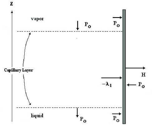
Figure 1: Interpretation of the surface tension in liquid-vapor interfaces as a layer of fluid endowed with internal capillarity.

Obviously, $\emph{P}_{{}_{0}}\,L$ is negligible. Let us denote

$$H=\int_{x_{3}^{v}}^{x_{3}^{l}}\lambda\,(\mathop{\mathrm{g}rad}\rho)^{2}\,h_{3}\,dx_{3},$$

the force per unit length; then $H$ represents the surface tension of the plane interface at equilibrium.

10 Practical calculation of the surface tension

By integrating Eq. (19) on the third coordinate line, the viscosity term being assumed negligible, we obtain

$$\lambda\,\Delta\rho=\frac{\partial}{\partial\rho}\left(\rho\int_{\rho_{v}}^{\rho}\frac{\emph{P - P}_{v}}{\rho^{2}}\,d\rho\right).$$ (23)

Let us notice that $\displaystyle\frac{\partial\emph{P}}{\partial\theta}\frac{\partial\theta}{\partial x_{3}}$ is negligible with respect to $\displaystyle\frac{\partial\emph{P}}{\partial\rho}\frac{\partial\rho}{\partial x_{3}}.$

Taking Eq. (21) into account, a further integration on the third coordinate leads to

$$\frac{\lambda}{2}(\mathop{\mathrm{g}rad}\rho)^{2}=2\frac{\lambda}{R_{m}}\int_{x_{3}^{v}}^{x_{3}}(\mathop{\mathrm{g}rad}\rho)^{2}h_{3}\,dx_{3}+\rho\int_{\rho_{v}}^{\rho}\frac{\emph{P - P}_{v}}{\rho^{2}}\,d\rho\,.$$ (24)

By denoting $x_{3}^{i}$ the third coordinate of the surface of equal density $\rho=\rho_{i}$, then for $x_{3}\in[x_{3}^{v},x_{3}^{i}]$, the term $\ \displaystyle 2\frac{\lambda}{R_{m}}\int_{x_{3}^{v}}^{x_{3}}(\mathop{\mathrm{g}rad}\rho)^{2}h_{3}\,dx_{3}\$ is negligible with respect to $\ \displaystyle\frac{\lambda}{2}\,(\mathop{\mathrm{g}rad}\rho)^{2}$; that is the case for $\displaystyle\rho_{i}=\frac{1}{2}\,(\rho_{v}+\rho_{l})$. For $\rho\in[\rho_{v},\rho_{i}]$,  Eq. (24) writes

$$\frac{\lambda}{2}(\mathop{\mathrm{g}rad}\rho)^{2}=\rho\int_{\rho_{v}}^{\rho}\frac{\emph{P - P}_{v}}{\rho^{2}}d\rho.$$

We obtain the same result for $\rho\in[\rho_{i},\rho_{l}]$ and finally,

$$H=\sqrt{2\lambda\,}\left(\int_{\rho_{v}}^{\rho_{i}}\sqrt{u\int_{\rho_{v}}^{u}\frac{\emph{P - P}_{v}}{\rho^{2}}d\rho}\ du+\int_{\rho_{i}}^{\rho_{l}}\sqrt{u\int_{\rho_{i}}^{u}\frac{\emph{P - P}_{l}}{\rho^{2}}d\rho\ }du\right).$$ (25)

Relation (25) expresses the surface tension of a liquid-vapor interface for motions compatible with the interface. Here P is not only a function of density but also temperature and varies according to the location of the point within the interface. The viscosity has explicitly disappeared in the expression of $H$ (the expression of $H$ does not explicitly take the viscosity into account). In the case of plane interface in isothermal equilibrium, the expression given by Rocard [9] is found again. The value of the internal capillarity constant can be numerically calculated on the basis of experimental values of $H$ and expressions of $P$. By injecting the value of $\lambda$ in Eq. (25), we can calculate surface tension for any dynamic temperature distribution.

Remark: Eq. (23) yields

$$\lambda\,\Delta\rho=\frac{\emph{P}}{\rho}-\frac{\emph{P}_{v}}{\rho_{v}}+\int_{\rho_{v}}^{\rho}\frac{\emph{P}}{\rho^{2}}d\rho$$

and we deduce

$$\int_{\rho_{v}}^{\rho_{l}}\frac{\emph{P}}{\rho^{2}}\,d\rho=\frac{\emph{P}_{v}}{\rho_{v}}-\frac{\emph{P}_{l}}{\rho_{l}}$$

which represents an invariant corresponding to motions compatible with the interface. This invariant leads to the equations (4-11) of [15] demonstrated in the specific case of an interface in isothermal equilibrium. The case of plane interface leads to the Maxwell equal area rule [9, 15].

11 Marangoni effect in liquid-vapor interfaces

Let us denote

$$H_{j}\left(x_{3}\right)=\int_{x_{3}^{j}}^{x_{3}}(\mathop{\mathrm{g}rad}\rho)^{2}h_{3}\,dx_{3},\qquad\mathrm{where}\quad j\in\{\emph{v},\emph{l}\}.$$

By using calculations as in Section 10, for example for $\ x_{3}\in[x_{3}^{v},x_{3}^{l}]$, we obtain

$$H_{v}(x_{3})=\sqrt{2\lambda\,}\left(\int_{\rho_{v}}^{\rho}\sqrt{u\int_{\rho_{v}}^{u}\frac{\emph{P - P}_{v}}{\rho^{2}}d\rho}\ du\right).$$

By injecting Eq. (22) into Eq. (23), we obtain:

$$\rho\,\mathbf{a}_{tg}=\frac{\lambda}{2}\,\text{grad}_{tg}(\mathop{\mathrm{g}rad}\rho)^{2}-\text{grad}_{tg}\left(\frac{2}{R_{m}}H_{j}(x_{3})\right)-\text{grad}_{tg}\emph{P}_{j}+2\mu(\mathop{\mathrm{d}iv}D)_{tg}.$$ (26)

Equation (18) and conditions on partial derivatives of velocity imply:

$$\int_{x_{3}^{v}}^{x_{3}^{l}}(\mathop{\mathrm{d}iv}D)_{tg}h_{3}\,dx_{3}=[De_{3}]_{x_{3}^{v}}^{x_{3}^{l}}\,.$$

Integration of Eq. (26) yields:

$$\frac{\lambda}{2}\int_{x_{3}^{v}}^{x_{3}^{l}}\text{grad}_{tg}(\mathop{\mathrm{g}rad}\rho)^{2}h_{3}\,dx_{3}+2[\mu De_{3}]_{x_{3}^{v}}^{x_{3}^{l}}=0\,.$$

Taking account of

$$\frac{\lambda}{2}\int_{x_{3}^{v}}^{x_{3}^{l}}\text{grad}_{tg}(\mathop{\mathrm{g}rad}\rho)^{2}h_{3}\,dx_{3}=\text{grad}_{tg}\left\{\lambda\int_{x_{3}^{v}}^{x_{3}^{l}}(\mathop{\mathrm{g}rad}\rho)^{2}h_{3}\,dx_{3}\right\},$$

we can conclude

$$\text{grad}_{tg}H+2[\mu De_{3}]_{v}^{l}=0\,.$$

If the viscosity stress tensor of the vapor bulk is supposed to be negligible, we get:

$$\text{grad}_{tg}H+2[\mu D^{l}e_{3}]=0\,.$$

This is the usual Marangoni condition for free boundary problems [6]. In the limit case when the viscosity coefficient is null (as for superfluid helium), the problem must be proposed in another way: the momentum associated with the interface can no longer be neglected and other physical effects must be taken into account [5]. We must note there exist other phenomenal presentations of the Marangoni effect (for example [40]), but to our knowledge, they all consider the interface as a discontinuous surface of the fluid medium. The calculations performed in the present text do not call upon the use of any linear approximations, and only take account of the various physical quantities describing liquid-vapor interfaces while working far from the critical temperature. The use of second gradient theory for representing interfaces has, of course, been considered by several authors. In [11, 41, 42, 43], their source is found to be in free energy which is more directly useable in case of isothermal flows.

12 Conclusion and further developments

As we have seen in this revisited version of [44], the second gradient theory, conceptually more straightforward than the Laplace theory can be used to build a theory of capillarity. Such a theory is able to take account of systems in which fluid interfaces are present. The internal capillarity associated with fluids is the simplest case. A mathematical limit analysis associated with the thickness of the interface when the size of the layer goes toward zero and the behavior of the layer between fluid phases yield the model of material surfaces. Such a theory is able to calculate the superficial tension as well in the case of thin interfaces as thick interfaces. The static model in continuum mechanics of second gradient theory is extended to dynamics. The equation of motion is able to induce a stress tensor. In the fluid case, the theory does not lead to an isotropic stress tensor.

Many developments have been done since paper [44] by the author:

It is possible to obtain the radius of nucleation of microscopic drops and bubbles and to develop a macroscopic theory as the Laplace theory of capillarity for curved interfaces [45]. The stability of interfaces is investigated with differential or partial derivative equations [46]. Classification of fluids endowed with internal capillarity is the extension of the classical fluid one’s [47].
In fact, contact forces are of a different nature than the ones associated with the Cauchy stress tensor. Classical conditions with the tetrahedron construction due to Cauchy are not efficient to study the non-linear behavior of fluids endowed with internal capillarity. We deduced contact forces concentrated on edges representing the boundaries of surfaces of separation. For example, such conditions are necessary to study the stability of thin films in contact with solid walls and the connection with the mean field molecular theories [48, 49, 50, 51, 52].
The model dynamically interprets phenomena in the vicinity of the critical point and authorizes an investigation - at least qualitative - of the dynamic change of phases between bulks in fluids or fluids mixtures [53, 54]. New mathematical equations associated with the hyperbolicity in continuous media can be considered in second gradient theory and consequently in internal capillarity [55, 56].
More recently, we must notice that fluids endowed with internal capillarity are able to model fluid layers at a scale of some nanometers and to recognize the disjoining pressure concept for very thin liquid films [52]. The model can be applied in vegetal biology to interpret the ascent of the crude sap in very high trees as sequoia and giant eucalyptus [57, 58]

References

- [1] R. Defay, I. Prigogine and A. Sanfeld, Surface Thermodynamics, J. Colloid Interf. Sci., 58 (1977) 498.
- [2] A. Sanfeld, Thermodynamics of Surfaces, in Physical Chemistry vol. 1, Academic press, New York (1971).
- [3] G. Emschwiller, Chimie Physique, P.U.F., Paris (1961).
- [4] S. Davis, Rupture of thin liquid films in Waves on Fluid Interface, R.E. Meyer, ed., Academic press, New York (1983).
- [5] L. Landau and E. Lifchitz, Fluids Mechanics, Mir, Moscow (1958).
- [6] A.K. Sen and S.H. Davis, Steady thermocapillarity flows in two-dimensional slots, J. Fluid Mech., 121 (1982) 163.
- [7] S. Ono and S. Kondo, Molecular theory of surface tension in liquid, in Structure of Liquids, S. Flügge, ed., Encyclopedia of Physics, X, Springer, Berlin, (1960).
- [8] V. Levitch, Physicochemical Hydrodynamics, Prentice-hall, New Jersey, (1962).
- [9] Y. Rocard, Thermodynamique, Masson, Paris, (1952).
- [10] J.W. Cahn and J.E. Hilliard, Free energy of a nonuniform system. III. Nucleation in a two-component incompressible fluid, J. Chem. Phys., 31 (1959) 688.
- [11] J.E. Dunn and J. Serrin, On the thermodynamics of interstitial working, Arch. Ration. Anal., 88 (1985) 95.
- [12] A. Brin, Contribution à l’étude de la couche capillaire et de la pression osmotique, Thesis, Paris, (1956).
- [13] J.S. Rowlinson and B. Widom, Molecular Theory of Capillarity, Clarenton Press, Oxford, (1982).
- [14] P.C. Hohenberg and B.I. Halpering, Theory of dynamic critical phenomena, Reviews of Modern Physics, 49 (1977) 435.
- [15] E.C. Aifantis and J.B. Serrin, The mechanical theory of fluid interfaces and Maxwell’s rule, J. Colloid Interf. Sci., 96 (1983) 517.
- [16] G. Bruhat, Cours de Physique Generale: Thermodynamique, Masson, Paris, (1968).
- [17] P. Casal, La theorie du second gradient et la capillarite, C.R. Acad. Sc. Paris, 274 (1972) 1571.
- [18] V. Bongiorno, L.E. Scriven and H.T. Davis, Molecular theory of fluid interfaces, J. Colloid Interf. Sci., 57 (1976) 462.
- [19] P. Casal and H. Gouin, Connection between the energy equation and the motion equation in korteweg theory of capillarity, C.R. Acad. Sc. Paris, 300 (1985) 231.
- [20] P. Casal and H. Gouin, Kelvin’s theorems and potential equation in Korteweg’s theory of capillarity, C.R. Acad. Sc. Paris, 300 (1985) 301.
- [21] H. Gouin, Dynamical surface tension and Marangoni effect for liquid-vapor interfaces in internal capillarity theory, C.R. Acad. Sc. Paris, 303 (1986) 5.
- [22] P. Casal, Capillarité interne en mécanique des milieux continus, C.R. Acad. Sc. Paris, 256 (1963) 3820.
- [23] J.D. van der Waals, Thermodynamique de la capillarité dans l’hypothèse d’une variation continue de densité, Arch. Néerlandaises, XXVIII (1894) 121.
- [24] D.J. Korteweg, Sur la forme que prennent les équations du mouvement des fluides si l’on tient compte des forces capillaires, Arch. Néerlandaises, II, VI (1901) 1.
- [25] M.E. Gurtin, Thermodynamics and the possibility of spatial interaction in elastic materials, Arch. Ration. Mech. Anal., 19 (1965) 339.
- [26] P. Germain, La méthode des puissances virtuelles en mécanique des milieux continus, Journal de Mécanique, 12 (1973) 235.
- [27] P. Casal, Principes variationnels en fluide compressible et en magné-todynamique des fluides, Journal de Mécanique, 5 (1966) 149.
- [28] R.L. Selinger and G.B. Whitham, Variational principles in continuum mechanics, Proc. Roy. Soc. A., 305 (1968) 1.
- [29] H. Gouin, Contribution à une étude géometrique et variationnelle des milieux continus, Thesis, Université d’Aix-Marseille, (1978).
- [30] H. Gouin, Exemples of non-conservative perfect fluid motions, Journal de Mécanique, 20 (1981) 273.
- [31] M. Ishi, Thermo-fluid Dynamic. Theory of Two-phase Flow, Eyrolles, Paris, (1975).
- [32] G. Birkhoff, Numerical fluid dynamics, SIAM Review, 25 (1983) 31.
- [33] J. Pratz, Contribution à la théorie du second gradient pour les milieux isotropes, Thesis, Université of Aix-Marseille, (1981).
- [34] J. Serrin, Mathematical principles of classical fluid dynamics, in Fluid Dynamics 1, S. Flügge, ed., Encyclopedia of Physics, VIII/1, Springer, Berlin, (1959).
- [35] C. Truesdell, Rational Thermodynamics, Mac Graw Hill, New York, (1969).
- [36] H. Gouin, Noether theorem in fluid mechanics, Mech. Res. Comm., 3 (1976) 151.
- [37] H. Gouin, Thermodynamic form of the equation of motion for perfect fluid of grade n, C.R. Acad. Sc. Paris, 305 II (1987) 833, arXiv:1006.0802.
- [38] G. Valiron, Equations fonctionnelles: Applications, Masson, Paris, (1950).
- [39] P. Germain, Mécanique des Milieux Continus, Masson, Paris, (1962).
- [40] L.E. Scriven, Dynamics of a fluid interface. Equation of motion for Newtonian surface fluids, Chem. Engng. Sci., 12 (1960) 98.
- [41] M. Slemrod, Admissibility criteria for propagating phase boundaries in a van der Waals fluid, Arch. Ration. Mech. Anal., 81 (1983) 301.
- [42] M. Slemrod, Dynamic phase transitions in a van der Waals fluid, J. Diff. Equ., 52 (1984) 1.
- [43] J. Dunn, Interstitial working and a nonclassical continuum thermodynamics in New perspectives in thermodynamics, ed., J. Serrin, Springer, Berlin, (1986) 187.
- [44] H. Gouin, Physicochemical Hydrodynamics, Series B, Physics, 174 (1986) 667.
- [45] F. dell’Isola, H. Gouin and P. Seppecher, Radius and surface tension of microscopic bubbles by second gradient theory, C.R. Sc. Paris, 320 IIb (1995) 211, arXiv:0808.0312.
- [46] H. Gouin and M. Slemrod, Stability of spherical isothermal liquid-vapor interfaces, Meccanica, 30 (1995) 305.
- [47] P. Casal and H. Gouin, Invariance properties of perfect fluids of grade n, Lecture Notes in Physics, 344, 85, Springer, Berlin (1989), arXiv:0803.3160.
- [48] H. Gouin, Energy of interaction between solid surface and liquids, Journal of Physical Chemistry, 102 (1998) 1212, arXiv:0801.4481.
- [49] H. Gouin and W. Kosinski, Boundary conditions for a capillary fluid in contact with a wall, Archives of Mechanics, 50 (1998) 907, arXiv:0802.1995.
- [50] H. Gouin and S. Gavrilyuk, Wetting problem for multicomponent fluid mixtures, Physica A, 268 (1999) 291, arXiv:0803.0275.
- [51] H. Gouin, Elastic effects of liquids on surface physics, Comptes Rendus Mécanique, 337 (2009) 218, arXiv:0905.0081.
- [52] H. Gouin, A mechanical model for the disjoining pressure, International Journal of Engineering Science, 47 (2009) 691, arXiv:0904.1809.
- [53] H. Gouin, Dynamic effects in gradient theory for fluid mixtures, IMA Volume in Mathematic and its Applications, 52 (1993) 111, arXiv:0804.0338.
- [54] H. Gouin and T. Ruggeri, Mixtures of fluids involving entropy gradients and accelerations waves in interfacial layers, European Journal of Mechanics/B, 24 (2005) 596, arXiv:0801.2096.
- [55] S. Gavrilyuk and H. Gouin, A new form of governing equations of fluids arising from Hamilton’s principle, International Journal of Engineering Science, 37 (1999) 1485, arXiv:0801.2333.
- [56] S. Gavrilyuk and H. Gouin, Symmetric form of governing equations for capillary fluids in Trends in applications of mathematics to mechanics, Ed. G. Iooss, O. Gu s, A. Nouri, ch.IX, 106 (2000) 306, Chapman & Hall/CRC, arXiv:0802.1670.
- [57] H. Gouin, A new approach for the limit to tree height using a liquid nanolayer model, Continuum Mechanics and Thermodynamics, 20 (2008) 317, arXiv:0809.3529.
- [58] H. Gouin, Liquid-solid interaction at nanoscale and its application in vegetal biology, Colloids and Surfaces A, 393 (2011) 17, arXiv:1106.1275.