On the polar degree of projective hypersurfaces

Abstract.

Given a hypersurface in the complex projective $n$-space we prove several known formulas for the degree of its polar map by purely algebro-geometric methods. Furthermore, we give formulas for the degree of its polar map in terms of the degrees of the polar maps of its components. As an application, we classify the plane curves with polar map of low degree, including a very simple proof of I. Dolgachev’s classification of homaloidal plane curves.

1. Introduction

Let $f$ be a homogeneous polynomial in $n+1$ variables defined over the field of complex numbers. In this note we analyze the relationship between the geometry of its zero scheme $D\subset\mathbb{P}^{n}$ and properties of its polar map $\nabla f\colon\mathbb{P}^{n}\dashrightarrow\mathbb{P}^{n}$, given by its partial derivatives. Easy cases are well understood: the hypersurface $D$ is smooth if and only if the polar map is a morphism; and $D$ has a non-vanishing Hessian if and only if $\nabla f$ is dominant. Nevertheless, there are classical questions still waiting for a satisfactory answer. For example, one asks for a classification of homaloidal hypersurfaces, that is, those whose polar map is birational. This is a natural problem which has received a lot of attention recently. We give a quick survey of its status.

A basic result towards the classification is that the answer depends only on the topology of its zero set. To be precise, if we let $d_{t}(D)$ or $d_{t}(f)$ denote the polar degree of $f$, defined as the topological degree of its polar map, then $d_{t}(f)=d_{t}(f_{\mathrm{red}})$ ([DP03, Cor. 2], [FP07]). So, for classification purposes, we may assume all hypersurfaces are reduced.

The plane case has been settled by I. Dolgachev and the complete list is quite neat [Dol00, Thm. 4]: a reduced homaloidal plane curve must be either the union of three non-concurrent lines; or a smooth conic; or the union of a smooth conic and a tangent line. On the other hand, the picture for higher dimensions is completely different: as it has been shown by C. Ciliberto, F. Russo and A. Simis, there are irreducible homaloidal hypersurfaces of any degree $\geq 2n-3$ for every $n\geq 3$ [CRS08, Thm. 3.13]. Interestingly enough, all these examples exhibit a common feature, to wit, a complicated singular locus, usually non-reduced. Actually, A. Dimca conjectured that do not exist homaloidal hypersurfaces of degree at least three with only isolated singularities whenever $n\geq 3$. There are some results giving plausibility to this, such as [Dim01, Thm. 9], [CRS08, Prop. 3.6] and [Ahm10, Cor. 3.5].

A bit more ambitiously, one may ask for formulas for the polar degree. And as we shall see in the sequel, there are plenty. For starters, we associate to a hypersurface $D$ of degree $k$ a foliation $\mathcal{F}$, now in $\mathbb{P}^{n+1}$, simply by taking the pencil generated by $f$ and $x_{n+1}^{k}$. Next, consider the Gauss map $\mathcal{G}_{\mathcal{F}}\colon\mathbb{P}^{n+1}\dashrightarrow\check{\mathbb{P}}^{n+1}$ of the foliation, $p\mapsto T_{p}\mathcal{F}$. The upshot is that the maps $\nabla f$ and $\mathcal{G}_{\mathcal{F}}$ have the same degree, that is,

$$d_{t}(D)=d_{t}(\mathcal{G}_{\mathcal{F}}).$$ (1)

This has already been shown in [FP07]. With hindsight, we realized that all polar degree formulas known to us can be derived from (1) by purely algebro-geometric methods, often with simpler proofs. One of the aims of this note is to show how this can be done.

Furthermore, it would be interesting to have formulas expressing the polar degree of a hypersurface in terms of that of its components, for this may help to reduce the classification problem to irreducible hypersurfaces. Such formulas actually do exist, as we shall prove below.

Let us describe the contents of this paper. We state our main results along the way.

In Section 2 we outline the basic theory of holomorphic foliations needed for the our purposes. We give a simple proof of (1) and from it we prove in Proposition 2.3 the first formula for the polar degree: given a reduced hypersurface $D\subset\mathbb{P}^{n}$ of degree $k$ with only isolated singularities,

$$\textstyle d_{t}(D)=(k-1)^{n}-\sum\mu_{p}$$ (2)

where $\mu_{p}$ is the Milnor number of the singularity.

Section 3 is devoted to the classification of plane polar maps with low degree. From identity (2) and elementary properties of the Milnor number we obtain in Theorem 3.1 a formula for the polar degree in terms of its subcurves: given reduced curves $C_{1},C_{2}\subset\mathbb{P}^{2}$ with no common components,

$$d_{t}(C_{1}\cup C_{2})=d_{t}(C_{1})+d_{t}(C_{2})+\#(C_{1}\cap C_{2})-1.$$ (3)

We emphasize that the intersection points in (3) are counted without multiplicities. This seems surprising at first sight, but ties up with the general philosophy that the polar degree depends more on the topology than on the algebra. From this Dolgachev’s classification of homaloidal plane curves follows easily, see Theorem 3.2. Next, we list all reduced curves with polar degree two (exactly 9 types) and three (exactly 31 types), see Theorems 3.3 and 3.4.

Back to the general case, we start Section 4 by showing that the polar degree can also be given as the top Chern class of the bundle of logarithmic differentials of a resolution of $D$; precisely, we prove in Proposition 4.1: let $\pi\colon X\to\mathbb{P}^{n}$ be an embedded resolution of singularities of $D$. Then, for a generic hyperplane $H\subset\mathbb{P}^{n}$,

$$\textstyle d_{t}(D)=\int_{X}c(\Omega^{1}_{X}(\log\pi^{*}(D+H))).$$ (4)

Again, this can be derived directly from (1), as it has been already noted in [FP07]. Now, by taking into account that there is a “Gauss-Bonnet theorem for a complement of a divisor” (see Remark 4.2), we obtain in Corollary 4.3 an algebraic proof of a nice formula by Dimca and Papadima [DP03, Thm. 1] relating the polar degree and the topological Euler characteristic of the complement of a generic hyperplane section:

$$d_{t}(D)=(-1)^{n}(1-e(D\setminus H)).$$ (5)

This allows one to compute the polar degree effectively, thanks to P. Aluffi’s algorithm for the computation of the Euler characteristic via Chern-Schwartz-MacPherson classes [Alu03], implemented in Macaulay2 [GS].

With identity (5) at hand, a straightforward use of inclusion-exclusion principle for the Euler characteristic yields a generalization of (3): given $D_{1},D_{2}$ any hypersurfaces in $\mathbb{P}^{n}$,

$$d_{t}(D_{1}\cup D_{2})=d_{t}(D_{1})+d_{t}(D_{2})+(-1)^{n}(e(D_{1}\cap D_{2}\setminus H)-1).$$ (6)

In fact, we have more general versions of formulas (5) and (6), concerning the projective degrees of the polar map; see Corollary 4.3 for more details. Notice that (3) follows immediately from (6), but our first proof is more elementary.

Finally, in Section 5, we give some applications. Building on examples given in [CRS08, Thm. 3.13] and inspired by formula (6), we show in Example 5.1 there are reduced homaloidal hypersurfaces in $\mathbb{P}^{n}$ of any degree $\geq 2$ for every $n\geq 3$, thus eliminating the bound $2n-3$ mentioned above. There is a catch, though: in contrast with theirs, our examples are reducible.

The polar degree of hypersurfaces in $\mathbb{P}^{n}$ with normal crossings is computed in Example 5.2; by specializing to hyperplanes, we compute in Example 5.3 the projective degrees of the standard Cremona transformation of $\mathbb{P}^{n}$ for any value of $n$, recovering a result proved by G. Gonzalez-Sprinberg and I. Pan in [GP06, Thm. 2].

Our last application is given in Example 5.4. Once more helped by (6), we present a somewhat short proof of one of the main results of [Bru07]: a collection of $r$ distinct hyperplanes in $\mathbb{P}^{n}$ is homaloidal if and only if $r=n+1$ and they are in general position.

Acknowledgments. We owe a great deal to Jorge V. Pereira for sharing many of his ideas and for pointing out some helpful references. We thank Giuseppe Borrelli, Eduardo Esteves, Marco Pacini, Ivan Pan and Israel Vainsencher for valuable discussions on the subject.

2. From foliations to polar maps

A codimension one singular holomorphic foliation, from now on just a foliation, $\mathcal{F}$ on $\mathbb{P}^{n}$ is determined by a line bundle $\mathcal{L}$ and an element $\omega\in\mathrm{H}^{0}(\mathbb{P}^{n},\Omega^{1}_{\mathbb{P}^{n}}\otimes\mathcal{L})$ satisfying

1. $\operatorname{codim}\operatorname{Sing}(\omega)\geq 2$ where $\operatorname{Sing}(\omega)=\{x\in\mathbb{P}^{n}\mid\omega(x)=0\}$;

2. $\omega\wedge d\omega=0$ in $\mathrm{H}^{0}(\mathbb{P}^{n},\Omega^{3}_{\mathbb{P}^{n}}\otimes\mathcal{L}^{\otimes 2}).$

The singular set of $\mathcal{F}$, for short $\operatorname{Sing}(\mathcal{F})$, is by definition equal to $\operatorname{Sing}(\omega)$. By Frobenius’ Theorem, the integrability condition (ii) determines in an analytic neighborhood of every point $p\in\mathbb{P}^{n}\setminus\operatorname{Sing}(\mathcal{F})$ a holomorphic fibration of codimension one with relative tangent sheaf coinciding with the subsheaf of $T\mathbb{P}^{n}$ determined by the kernel of $\omega$. Analytic continuation of the fibers of this fibration describes the leaves of $\mathcal{F}$.

One of the most basic invariants attached to an isolated singularity of a foliation $\mathcal{F}$ is its multiplicity $\mu_{p}(\mathcal{F})$, defined as the intersection multiplicity at $p$ of the zero section of $\Omega^{1}_{\mathbb{P}^{n}}\otimes\mathcal{L}$ with the graph of $\omega$. Thus, if $\omega_{p}=\sum_{i=1}^{n}a_{i}dx_{i}$ is a local $1$–form defining $\mathcal{F}$ in a neighborhood of $p$, then

$$\mu_{p}(\mathcal{F})=\dim_{\mathbb{C}}\frac{\mathcal{O}_{p}}{(a_{1},\dots,a_{n})}.$$

The degree of a foliation of $\mathbb{P}^{n}$ is geometrically defined as the number of tangencies of $\mathcal{F}$ with a generic line $\mathbb{P}^{1}\subset\mathbb{P}^{n}$. If $\iota\colon\mathbb{P}^{1}\to\mathbb{P}^{n}$ is the inclusion of such a line, then the degree of $\mathcal{F}$ is the degree of the zero divisor of the twisted $1$-form $\iota^{*}\omega\in\mathrm{H}^{0}(\mathbb{\mathbb{P}}^{1},\Omega^{1}_{\mathbb{P}^{1}}\otimes\mathcal{L}_{|\mathbb{P}^{1}})$. Since $\Omega^{1}_{\mathbb{P}^{1}}=\mathcal{O}_{\mathbb{P}^{1}}(-2)$ the degree of $\mathcal{F}$ is just $\deg(\mathcal{L})-2$.

It follows from Euler sequence that a $1$-form $\omega\in\mathrm{H}^{0}(\mathbb{P}^{n},\Omega_{\mathbb{P}^{n}}^{1}(\deg(\mathcal{F})+2))$ can be interpreted as a homogeneous $1$-form on $\mathbb{C}^{n+1}$, still denoted by $\omega$,

$$\omega=\sum_{i=0}^{n}A_{i}dx_{i}$$

with the $A_{i}$ being homogeneous polynomials of degree $\deg(\mathcal{F})+1$ and satisfying Euler’s relation $i_{R}\omega=0,$ where $i_{R}$ stands for the interior product with the radial vector field $R=\sum_{i=0}^{n}x_{i}\frac{\partial}{\partial x_{i}}$.

The Gauss map of a foliation $\mathcal{F}$ of $\mathbb{P}^{n}$ is the rational map

$$\mathcal{G}_{\mathcal{F}}\colon\mathbb{P}^{n} \dashrightarrow \check{\mathbb{P}}^{n}\,$$

$$p \mapsto T_{p}\mathcal{F}$$

where $T_{p}\mathcal{F}$ is the tangent space of the leaf of $\mathcal{F}$ through $p$. If we interpret $(dx_{0}:\cdots:dx_{n})$ as projective coordinates of $\check{\mathbb{P}}^{n}$, then the Gauss map of the foliation $\mathcal{F}$ is just the rational map $p\mapsto\left(A_{0}(p):\cdots:A_{n}(p)\right).$

Let $H=\iota(\mathbb{P}^{n-1})\subset\mathbb{P}^{n}$ be a hyperplane given by the inclusion $\iota\colon\mathbb{P}^{n-1}\to\mathbb{P}^{n}$. If $\iota^{*}(\omega)$ is identically zero, we say that $H$ is invariant by $\mathcal{F}$; otherwise, after dividing the $1$–form $\iota^{*}(\omega)$ by a codimension one singular set if necessary, we consider the restriction $\mathcal{F}_{|H}$ as the foliation defined by this $1$–form. The following well-known lemma (cf. [CLS92]), which follows from Sard’s Theorem applied to $\mathcal{G}_{\mathcal{F}}$, will be useful to obtain some information for the topological degree of $\mathcal{G}_{\mathcal{F}}$.

Lemma 2.1.

If $H\subset\mathbb{P}^{n}$ is a generic hyperplane and $\mathcal{F}$ is a foliation on $\mathbb{P}^{n}$, then the degree of $\mathcal{F}_{|H}$ is equal to the degree of $\mathcal{F}$ and, moreover,

$$\operatorname{Sing}(\mathcal{F}_{|H})=(\operatorname{Sing}(\mathcal{F})\cap H)\cup\mathcal{G}_{\mathcal{F}}^{-1}(H)$$

with $\mathcal{G}_{\mathcal{F}}^{-1}(H)$ being finite and all the corresponding singularities of $\mathcal{F}_{|H}$ have multiplicity one.

Now let $D\subset\mathbb{P}^{n}$ be a hypersurface given by a homogeneous polynomial $f\in\mathbb{C}[x_{0},\dots,x_{n}]$ of degree $k$. We denote by $d_{t}(D)$ or $d_{t}(f)$ its polar degree, defined as the topological degree of its polar map

$$\nabla f\colon\mathbb{P}^{n} \dashrightarrow \mathbb{P}^{n}$$

$$x \mapsto (f_{x_{0}}(x):\cdots:f_{x_{n}}(x)).$$

Since the polar degree depends only on the zero locus of $f$ (cf. [DP03, FP07]) we may suppose $f$ reduced.

We associate to this hypersurface a foliation $\mathcal{F}$ in $\mathbb{P}^{n+1}$ defined by the pencil generated by $f$ and $x_{n+1}^{k}$, that is, the foliation induced by the $1$-form

$$\omega=x_{n+1}df-kfdx_{n+1}.$$

Remark 2.2.

Let $\mathcal{G}_{\mathcal{F}}$ be the Gauss map associated to this foliation

$$\mathcal{G}_{\mathcal{F}}\colon\mathbb{P}^{n+1} \dashrightarrow \mathbb{P}^{n+1}$$

$$x \mapsto (x_{n+1}f_{x_{0}}(x):\cdots:x_{n+1}f_{x_{n}}(x):-kf(x)).$$

If $\rho(x_{0}:\cdots:x_{n}:x_{n+1})=(x_{0}:\cdots:x_{n})$ is the projection with center at $p=(0:\cdots:0:1)$, we see that the rational maps $\mathcal{G}_{\mathcal{F}}$ and $\nabla f$ fit in the commutative diagram below.

A simple computation shows that the restriction of $\rho$ to a fiber of $\mathcal{G}_{\mathcal{F}}$ induces an isomorphism to the corresponding fiber of $\nabla f$ and so their topological degrees coincide, that is, $d_{t}(f)=d_{t}(\mathcal{G}_{\mathcal{F}})$. This is a particular case of [FP07, Thm. 2] where higher degrees are also considered.

With this at hand we are able to recover a formula for the polar degree of hypersurfaces with only isolated singularities. The main invariant to be considered here is the Milnor number

$$\mu_{p}(f)=\dim_{\mathbb{C}}\frac{\mathcal{O}_{p}}{(\tilde{f}_{x_{1}},\dotsc,\tilde{f}_{x_{n}})}$$

where $\tilde{f}$ is the germ of $f$ at $p$.

Proposition 2.3.

Let $D\subset\mathbb{P}^{n}$ be a hypersurface with isolated singularities, given by a reduced polynomial $f\in\mathbb{C}[x_{0},\dots,x_{n}]$ of degree $k$. Then

$$\textstyle d_{t}(D)=(k-1)^{n}-\sum\mu_{p}(f).$$

Proof.

Consider the foliation $\mathcal{F}$ on $\mathbb{P}^{n+1}$ induced by the $1$-form

$$\omega=x_{n+1}df-kfdx_{n+1}.$$

Notice that all the singularities of this foliation are contained in $D$.

It follows from Lemma 2.1 that the degree $d_{t}(\mathcal{G}_{\mathcal{F}})$ of the Gauss map is given by the number of isolated singularities of $\mathcal{F}|_{H}$ away from $\operatorname{Sing}(\mathcal{F})$, where $H$ is generic hyperplane on $\mathbb{P}^{n+1}$.

Denote by $h=x_{n+1}|_{H}$ and $\tilde{f}=f|_{H}$ the restrictions to $H$. Thus $\mathcal{F}|_{H}$ is induced by the $1$–form

$$\eta=hd\tilde{f}-k\tilde{f}dh.$$

Let us suppose ${h=\sum_{i=1}^{n}a_{i}x_{i}}$ with $a_{0}\neq 0$. On the one hand the singular set of $\eta$ outside $Z(h)$ is given by $\mathcal{G}_{\mathcal{F}}^{-1}(H)\cup\operatorname{Sing}{D}$; and on the other hand it is also given by the intersection of $n$ hypersurfaces of degree $k-1$

$$\bigcap_{i=1}^{n}Z(a_{0}f_{x_{i}}-a_{i}f_{x_{0}})$$

so by Bézout’s Theorem we get $d_{t}(\mathcal{G}_{\mathcal{F}})+\sum\mu_{p}(f)=(k-1)^{n}.$ Now the proposition follows from Remark 2.2. ∎

For different proofs see [DP03, p. 487] and [Huh11, Example 11].

3. Plane polar maps of low degree

The main result of this section is a formula for computing the polar degree of a plane curve in terms of that of its components. Once we have established that, we present the classification of all reduced plane curves with polar degree less or equal than three.

Theorem 3.1.

1. Given an irreducible curve $C\subset\mathbb{P}^{2}$ of degree $k$, then

   $$\textstyle d_{t}(C)=k-1+2p_{g}+\sum(r_{p}-1)$$ (7)

   where $p_{g}$ is the geometric genus and $r_{p}$ is the number of branches at $p$.

2. Given two reduced curves $C,D$ in $\mathbb{P}^{2}$ with no common components, we have

   $$d_{t}(C\cup D)=d_{t}(C)+d_{t}(D)+\#(C\cap D)-1.$$ (8)

Proof.

A more general version of (7) already appeared in [Dol00] but we give the argument for the reader’s convenience. Since $C$ is irreducible, the genus formula gives

$$\textstyle p_{g}=(k-1)(k-2)/2-\sum\delta_{p}$$

where $\delta_{p}=\dim_{\mathbb{C}}\widetilde{\mathcal{O}_{p}}/\mathcal{O}_{p}$ is the codimension of the local ring $\mathcal{O}_{p}$ in its normalization. Now combine this with the Milnor Formula

$$\mu_{p}=2\delta_{p}-r_{p}+1$$

and Proposition 2.3 to get the result.

Let’s prove (8). Write $C=Z(f)$, $D=Z(g)$ and let $k,l$ be their degrees. By Proposition 2.3, the polar degree of the product $fg$ is $(k+l-1)^{2}-\sum\mu_{p}(fg).$ Rewriting,

$$d_{t}(fg)=(k-1)^{2}+(l-1)^{2}+2kl-1-\!\!\!\sum_{p\in C\cap D}\!\!\!\mu_{p}(fg)-\!\!\!\sum_{p\in C\setminus D}\!\!\!\mu_{p}(f)-\!\!\!\sum_{p\in D\setminus C}\!\!\!\mu_{p}(g).$$ (9)

Since $fg$ is reduced, we have the well-known identity [CA00, Cor. 6.4.4]

$$\mu_{p}(fg)=\mu_{p}(f)+\mu_{p}(g)+2\operatorname{I}_{p}(f,g)-1$$

where $\operatorname{I}_{p}$ is the intersection multiplicity. Plugging this into (9) and applying Proposition 2.3

$$d_{t}(fg)=d_{t}(f)+d_{t}(g)+2kl-2\!\!\!\sum_{p\in C\cap D}\!\!\!\operatorname{I}_{p}(f,g)+\#(C\cap D)-1$$

and hence by Bézout’s Theorem we are done. ∎

Theorem 3.1 makes the classification of homaloidal plane curves amazingly simple, since the polar degree never decreases whenever a new component is added. We are ready to prove the celebrated Dolgachev’s theorem [Dol00, Thm. 4]:

Theorem 3.2.

A reduced homaloidal curve in the projective plane must be one the following:

1. Three nonconcurrent lines.

2. A smooth conic.

3. A smooth conic and a tangent line.

Proof.

Let $C\subset\mathbb{P}^{2}$ be a reduced homaloidal curve. Then it follows from equations (7) and (8) that $C$ can have only lines and at most one irreducible conic as components. If $C$ has a conic, then (8) imposes $C$ can have at most one line, which must meet the conic at a single point.

Assume now our curve has only lines. These cannot be all concurrent, for otherwise the polar degree is zero by (8). If $C$ is the union of three nonconcurrent lines, then $d_{t}=1$ by (8). Finally, if $C$ has more than three lines, not all concurrent, once more formula (8) gives $d_{t}>1$. ∎

The polar degree two case is also quite easy.

Theorem 3.3.

A reduced plane curve with polar degree two must be one of the following:

1. Three concurrent lines and a fourth line not meeting the center point.

2. A smooth conic and a secant line.

3. A smooth conic, a tangent and a line passing thru the tangency point.

4. A smooth conic and two tangent lines.

5. Two smooth conics meeting at a single point.

6. Two smooth conics meeting at a single point and the common tangent.

7. An irreducible cuspidal cubic.

8. An irreducible cuspidal cubic and its tangent at the smooth flex point.

9. An irreducible cuspidal cubic and its tangent at the cusp.

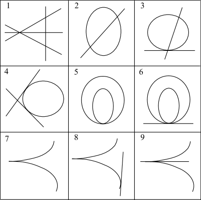
Figure 1. Plane curves with $d_{t}=2$.

Proof.

Such a curve cannot have components of degree greater than 3. From (7) we see that an irreducible cubic with $d_{t}=2$ must be cuspidal; and in view of (8) we may attach to it at most one line and they ought to meet at a single point. This accounts for the last three cases in the statement.

The remaining cases, unions of lines and conics, may be analyzed by inspection and are exactly the ones listed above. ∎

We proceed to classify the plane curves with polar degree three.

Theorem 3.4.

A reduced plane curve with polar degree three must be one of the 31 types shown in Figure 2.

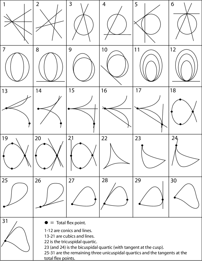
Figure 2. Plane curves with polar degree three.

Proof.

Here irreducible quartics will hop in but only cuspidal rational ones are allowed in view of equation (7). As before, we may attach to such a quartic a tangent line but only at total flex points. A neat list of all cuspidal rational plane quartics and their flex points can be found in [Moe08] (see also [Nam84]): up to projective equivalence there are exactly five, labeled 22, 23, 25, 27 and 30 in Figure 2.

Besides, we have to deal with unions of cubics, conics and lines. Keeping an eye in (7) and (8), all it takes is a careful analysis of the possible configurations and there is not much to say about it, except for the case of cubics and conics, which deserves more attention.

Let $C$ be a conic and let $D$ be a cubic, both irreducible. Since the conic is homaloidal, it follows from equation (8),

$$d_{t}(C\cup D)=d_{t}(D)+\#(C\cap D).$$

Since smooth and nodal cubics have polar degree $\geq 3$, we see there is only one possible case, namely, the cubic must be cuspidal and it must intersect the conic at a single point. This case is missing in Figure 2, for a very simple reason: this configuration does not exist! Although we believe this is well-known we are obliged to give a proof, for we lack a suitable reference.

Let $D$ be a cuspidal cubic and let us show that $C$ and $D$ cannot meet at a point with multiplicity six. By tensorizing the exact sequence that defines the ideal sheaf of $D$ by $\mathcal{O}_{\mathbb{P}^{2}}(2)$, we get

$$0\longrightarrow\mathcal{O}_{\mathbb{P}^{2}}(-1)\longrightarrow\mathcal{O}_{\mathbb{P}^{2}}(2)\longrightarrow i_{*}\mathcal{O}_{D}(2)\longrightarrow 0$$

and the long exact sequence in cohomology yields an isomorphism

$${\mathrm{H^{0}}}(\mathbb{P}^{2},\mathcal{O}_{\mathbb{P}^{2}}(2))\longrightarrow{\mathrm{H^{0}}}(D,\mathcal{O}_{D}(2)).$$

Hence, if a conic meets $D$ at a point $p$ with multiplicity six, this conic is unique. If $p$ is the cusp or the flex, then this conic is the double tangent line. Assume $p$ is neither the cusp nor the flex. Let $L$ be the tangent line at $p$ and write $L\!\cdot\!D=2p+q$. If there were a conic intersecting $D$ at $p$ with multiplicity six, we would get a linear equivalence $4p+2q\sim 6p,$ and hence $2p\sim 2q$, in $D\setminus\{c\}$, where $c$ denotes the cusp. Let $2q+r$ the divisor defined by the restriction on the tangent at $q$. Then $2p+q\sim 2q+r$ and thus $q\sim r$ in $D\setminus\{c\}$. This implies that $q=r$ (see [Har77, Example 6.11.4]). Therefore $q$ would be the flex point of $D$. But $D$ has no points $p$ for which the tangent line passes through the flex point, as can be checked by direct computation or, better, by a simple argument with the dual curve of $D$, which is also a cuspidal cubic. ∎

4. Logarithmic differential forms and the Euler characteristic

In this section we show that the formula (5) of Dimca and Papadima, which relates the polar degree of a hypersurface with the topological Euler characteristic of its affine part, can also be obtained by algebraic methods. As a consequence, we give a generalization of equation (8) for higher dimensions.

Let $X$ be a smooth projective variety of dimension $n$. We say that a divisor $D=\sum D_{i}$ of $X$ has normal crossings if $D$ is reduced, each component $D_{i}$ is smooth and at each point of intersection of some of the divisors $D_{i}$, say $D_{1},\dots,D_{k}$, there are local analytic coordinates $z_{1},\dots,z_{n}$ for $X$ so that $D_{i}$ is given by $z_{i}=0$ for $i=1,\dots,k$.

Let us suppose $D$ reduced. We define the sheaf of logarithmic differentials $\Omega^{1}_{X}(\log D)$ as a subsheaf of the sheaf $\Omega^{1}_{X}(D)$ of $1$-forms with poles at most on $D$ and of order one. This sheaf is the image of the natural map $\Omega_{X}^{1}\otimes\mathcal{O}_{X}^{\oplus n}\to\Omega^{1}_{X}(D)$, which is given by the inclusion $\Omega_{X}^{1}\to\Omega^{1}_{X}(D)$ and by the homomorphisms $\mathcal{O}_{X}\to\Omega^{1}_{X}(D)$ sending $1\mapsto d\log f_{i}$, where $f_{i}$ is a local equation of $D_{i}$. The reducedness assumption on $D$ is not essential here, for the differential logarithmic of a power of a function is a multiple constant of the differential logarithmic of the function. So $D$ and $D_{\mathrm{red}}$ define the same sheaf $\Omega^{1}_{X}(\log D)$. A basic known fact is that if $D$ has normal crossings, then the sheaf $\Omega^{1}_{X}(\log D)$ is locally free of rank $n$.

It has been shown in [FP07] that the polar degree can also be given as the degree of the total Chern class, denoted here by $c(\cdot)$, of the bundle of logarithmic differentials of a resolution of $D$, as we shall review now.

Proposition 4.1.

Let $D\subset\mathbb{P}^{n}$ be a reduced hypersurface and $\pi\colon X\to\mathbb{P}^{n}$ be an embedded resolution of singularities of $D$ so that the total transform $\pi^{*}D$ has normal crossings. Then, for a generic hyperplane $H\subset\mathbb{P}^{n}$,

$$\textstyle d_{t}(D)=\int_{X}c(\Omega^{1}_{X}(\log\pi^{*}(D+H))).$$ (10)

Proof.

This equality is a consequence of the Remark 2.2. We sketch the argument in the next few lines for the convenience of the reader.

Suppose $D$ is given by a homogeneous polynomial $f\in\mathbb{C}[x_{0},\dots,x_{n}]$ of degree $k$. Let $\mathcal{F}$ be the foliation on $\mathbb{P}^{n+1}$ induced by the rational $1$-form

$$\omega=\frac{df}{f}-k\frac{dx_{n+1}}{x_{n+1}}$$

and $\mathcal{G}_{\mathcal{F}}$ its Gauss map. By Lemma 2.1, $d_{t}(\mathcal{G}_{\mathcal{F}})$ coincides with the number of isolated singularities of $\mathcal{F}|_{\mathbb{P}^{n}}$ that are not singularities of $\mathcal{F}$; here, $\mathcal{F}|_{\mathbb{P}^{n}}$ is the restriction of $\mathcal{F}$ to a generic $\mathbb{P}^{n}\subset\mathbb{P}^{n+1}$. Since all the singularities of $\mathcal{F}$ are contained in $Z(x_{n+1}f)$ we have just to count the isolated singularities of $\mathcal{F}|_{\mathbb{P}^{n}}$ away from $Z(x_{n+1}f)$. The intersection in $\mathbb{P}^{n+1}$ of $Z(x_{n+1}f)$ and a generic $\mathbb{P}^{n}$ is isomorphic to the union of $D$ with a generic hyperplane $H\subset\mathbb{P}^{n}$. Thus the rational $1$-form $\omega|_{\mathbb{P}^{n}}$ can be viewed as an element of ${\rm{H^{0}}}(\mathbb{P}^{n},\Omega_{\mathbb{P}^{n}}^{1}(\log(D+H)))$. Since $\pi$ is an embedded resolution for $D$, Bertini’s Theorem implies that it is also an embedded resolution of $D\cup H$ and therefore $\Omega^{1}_{X}(\log\pi^{*}(D+H))$ is locally free. Assuming the singular scheme of $\pi^{*}\omega|_{\mathbb{P}^{n}}\in\mathrm{H}^{0}(X,\Omega_{X}^{1}(\log\pi^{*}(D+H)))$ has just a zero-dimensional part, its length is measured by the top Chern class of $\Omega^{1}_{X}(\log\pi^{*}(D+H))$. And the latter assumption follows from the fact that the residues of $\pi^{*}\omega|_{\mathbb{P}^{n}}$ on each irreducible component of the support of $\pi^{*}(D+H)$ are non-zero. For details see [FP07, Lemmas 3 and 4]. ∎

Remark 4.2.

Let $D$ be a smooth projective variety. The topological Euler characteristic of $D$ is computed by the degree of the Chern total class of the tangent bundle of $D$, that is,

$$\textstyle e(D)=\int_{D}c(TD).$$

This is the Gauss-Bonnet theorem. For the case that $D$ is a divisor with normal crossings of a smooth variety $X$, we have the following version:

$$\textstyle e(X\setminus D)=(-1)^{n}\int_{X}c(\Omega^{1}_{X}(\log D)).$$ (11)

Here, $X\setminus D$ is complement of the support of $D$. This has been proved by R. Silvotti [Sil96, Thm. 3.1] and recovered by P. Aluffi [Alu99, § 2.2] (along the way of his characterization of Chern-Schwartz-MacPherson classes), but both were predated by Y. Norimatsu [Nor78], a two-page gem that apparently had fallen into oblivion.

Let $D=Z(f)\subset\mathbb{P}^{n}$ be a hypersurface and consider its polar map $\nabla f\colon\mathbb{P}^{n}\dashrightarrow\check{\mathbb{P}}^{n}$. For each $i=0,\dots,n-1$, we denote by $d_{i}(D)$ the $i$-th projective degree of the polar map, defined as the degree of the closure of the algebraic set $\nabla f|_{U}^{-1}(L_{i})$, where $L_{i}\subset\check{\mathbb{P}}^{n}$ is a generic linear subspace of dimension $i$ and $U\subset\mathbb{P}^{n}$ is the Zariski open set where the polar map is regular. Notice that $d_{0}(D)$ is just the polar degree $d_{t}(D)$. It follows from [FP07, Cor. 2] that $d_{i}(D)$ coincides with the topological degree of the Gauss map of the restriction of the foliation $\mathcal{F}$ to a generic $\mathbb{P}^{n+1-i}\subset\mathbb{P}^{n+1}$, that is, $d_{i}(D)=d_{t}(\mathcal{G}_{\mathcal{F}|_{\mathbb{P}^{n+1-i}}}).$ Since $\mathcal{F}|_{\mathbb{P}^{n+1-i}}$ is the foliation associated to the divisor $D\cap\mathbb{P}^{n-i}$ for a generic $\mathbb{P}^{n-i}\subset\mathbb{P}^{n}$, it follows from Remark 2.2 that

$$d_{i}(D)=d_{t}(D\cap\mathbb{P}^{n-i}).$$ (12)

We are ready to give formulas relating the projective degrees of the polar map with the Euler characteristic.

Corollary 4.3.

Let $\mathbb{P}^{i},H\subset\mathbb{P}^{n}$ denote a generic linear subspace of dimension $i$ and a generic hyperplane, respectively.

1. Given a hypersurface $D\subset\mathbb{P}^{n}$, we have

   $$d_{i}(D)=(-1)^{n-i}(1-e(D\cap\mathbb{P}^{n-i}\setminus H))$$ (13)

   for $i=0,\dots,n-1$.

2. Given two hypersurfaces $D_{1},D_{2}\subset\mathbb{P}^{n}$, we have

   $$d_{i}(D_{1}\cup D_{2})=d_{i}(D_{1})+d_{i}(D_{2})+(-1)^{n-i}(e(D_{1}\cap D_{2}\cap\mathbb{P}^{n-i}\setminus H)-1)$$ (14)

   for $i=0,\dots,n-1$.

Proof.

In view of (12), it is enough to prove both assertions for $i=0$.

Let us prove that formula (13) holds for $i=0$. We may assume $D$ reduced. Let $\pi\colon X\to\mathbb{P}^{n}$ be an embedded resolution of singularities of $D$ such that $\pi^{*}D$ has normal crossings. Hence it follows from (10) and (11) that

$$(-1)^{n}d_{t}(D) =\textstyle(-1)^{n}\int_{X}c(\Omega^{1}_{X}(\log\pi^{*}(D+H)))$$

$$=e(X\setminus\pi^{*}(D+H))$$

$$=e(\mathbb{P}^{n}\setminus(D+H))$$

$$=1-e(D\setminus H)$$

where in the last equality have used $e(\mathbb{P}^{n})=n+1$ and the inclusion-exclusion principle for the Euler characteristic of algebraic varieties.

Finally, (14) follows from (13) and straightforward manipulations using inclusion-exclusion. ∎

Dimca and Papadima [DP03, Thm. 1] proved formula (13) for $i=0$, by using topological methods. The generalization for higher values of $i$ has been proved by Huh [Huh11, Thm. 8] quite recently. The expression (13) written here is slightly different from theirs. Furthermore, we point out that an identity for the polar degree similar to (14) has appeared in [Dim01, Prop. 5], but only for complete intersections.

Remark 4.4.

Let $D_{1},D_{2}\subset\mathbb{P}^{n}$ be hypersurfaces with no common components. It would be interesting to know whether the ‘correction term’ in (14):

$$(-1)^{n}(e(D_{1}\cap D_{2}\setminus H)-1)$$

is always non-negative, as this would reduce the classification of homaloidal hypersurfaces to the irreducible ones. That is the case in all examples we have checked. If that were the case in general, then we would have the inequality

$$d_{t}(D_{1}\cup D_{2})\geq\max\{d_{t}(D_{1}),d_{t}(D_{2})\}$$

proved in [FP07, Cor. 3] using foliations.

5. Applications

Example 5.1.

Starting with a hypersurface $D$ of degree $d$ in $\mathbb{P}^{n}$, there is a very simple way to construct another hypersurface $Y$, now of degree $d+1$ and sitting in $\mathbb{P}^{n+1}$, with the same polar degree: let $C,L\subset\mathbb{P}^{n+1}$ be the projective cone over $D$ and a generic hyperplane respectively and take $Y$ as their union. Since cones and hyperplanes have null polar degree and $C\cap L$ is isomorphic to $D$, equations (14) and (13) yield

$$d_{t}(Y) =d_{t}(C)+d_{t}(L)+(-1)^{n+1}(e((C\cap L)\setminus H)-1)$$

$$=(-1)^{n}(1-e(D\setminus h))$$

$$=d_{t}(D)$$

where $H$ and $h$ stand for generic hyperplanes in $\mathbb{P}^{n+1}$ and $\mathbb{P}^{n}$, respectively.

As a consequence, let us show that there are homaloidal reduced hypersurfaces in $\mathbb{P}^{n}$ for all $n\geq 3$ and of any degree $\geq 2$. Indeed, this is already known for $n=3$ [CRS08, Thm. 3.13] and so our construction gives homaloidal hypersurfaces in $\mathbb{P}^{4}$ for any degree $\geq 3$. As for degree two, we already know that smooth quadrics are always homaloidal, so we are done for $n=4$. Now one has just to workout the same reasoning for higher values of $n$.

The same construction gives a family of counter-examples for the Hesse’s problem (see [CRS08]), namely, hypersurfaces with vanishing Hessian that are not cones: one has only to notice that null Hessian is equivalent to polar degree zero and that if $D$ is not a cone, then $Y$ is not a cone as well.

Example 5.2.

Let $D=\sum_{i=1}^{r}D_{i}$ be a reduced divisor in $\mathbb{P}^{n}$ with normal crossings. Let $H\subset\mathbb{P}^{n}$ be a generic hyperplane. From the exact sequence of locally free sheaves on $\mathbb{P}^{n}$

$$0\to\Omega_{\mathbb{P}^{n}}^{1}\to\Omega_{\mathbb{P}^{n}}^{1}(\log(D+H))\to\oplus_{i}\mathcal{O}_{D_{i}}\oplus\mathcal{O}_{H}\to 0$$

and from Euler’s exact sequence

$$0\to\Omega_{\mathbb{P}^{n}}^{1}\to\mathcal{O}_{\mathbb{P}^{n}}(-1)^{\oplus n+1}\to\mathcal{O}_{\mathbb{P}^{n}}\to 0$$

we get, by Whitney’s formula and Proposition 4.1, that

$${\textstyle d_{t}(D)=\int_{\mathbb{P}^{n}}c(\Omega_{\mathbb{P}^{n}}^{1}(\log(D+H)))}=\left[\frac{(1-h)^{n}}{(1-k_{1}h)\dotsb(1-k_{r}h)}\right]_{n}$$ (15)

where $[\cdot]_{n}$ stands for the coefficient of $h^{n}$ and $k_{i}$ is the degree of $D_{i}$. For $r=2$,

$$d_{t}(D_{1}\cup D_{2})=d_{t}(D_{1})+d_{t}(D_{2})+q$$

where

$$q=\begin{cases}\displaystyle\frac{k_{2}(k_{1}-1)^{n}-k_{1}(k_{2}-1)^{n}}{k_{1}-k_{2}}&\text{if $k_{1}\neq k_{2}$}\\[11.38092pt] (k-1)^{n}(nk+k-3)&\text{if $k=k_{1}=k_{2}$}.\end{cases}$$

Here the correction term is always non-negative.

Example 5.3.

For a collection of $r$ hyperplanes in $\mathbb{P}^{n}$ in general position, a simple calculation from (15) yields

$$d_{t}=\begin{cases}0&\text{if $r\leq n$}\\ \binom{r-1}{n}&\text{if $r\geq n+1$}\end{cases}$$ (16)

so the polar map is birational if and only if $r=n+1$. In that case the map is, up to change of coordinates, the standard Cremona transformation $\phi\colon\mathbb{P}^{n}\dashrightarrow\mathbb{P}^{n}$, given as the polar map associated to $f=x_{0}\cdots x_{n}$. Now, identities (12) and (16) together yield expressions for the projective degrees of this map, namely

$$\textstyle d_{i}(\phi)=\binom{n}{n-i}$$

for $i=0,\dots,n-1$. These numbers have also been obtained by G. Gonzalez-Sprinberg and I. Pan [GP06, Thm. 2] by applying methods of toric geometry.

Example 5.4.

The first result of the last example holds in more generality. In fact, A. Bruno [Bru07, Thm. A] proved: a collection of $r$ distinct hyperplanes in $\mathbb{P}^{n}$ is homaloidal if and only if $r=n+1$ and they are in general position. We offer an alternative proof, based on formula (14).

Indeed, if $r\leq n+1$ and they are not in general position, then the arrangement is a cone, so the polar degree is zero; and we have seen in Example 5.3 that $n+1$ hyperplanes in general position is homaloidal. So, if $D$ is the union of $r$ hyperplanes, it suffices to show that $d_{t}(D)\geq 2$ whenever $r\geq n+2$ and $D$ is not a cone. The conclusion goes by induction on $n$. For $n=1$ this is immediate, so we assume $n\geq 2$ and $D$ is not a cone. Let $D^{\prime}$ be the union of the first $r-1$ hyperplanes and $H_{r}$ be the last one. By equation (14)

$$d_{t}(D)=d_{t}(D^{\prime})+d_{t}(H_{r})+(-1)^{n}(e(D^{\prime}\cap H_{r}\setminus H)-1).$$

Now, $D^{\prime}\cap H_{r}$ is an arrangement of $r-1$ hyperplanes in $H_{r}$. By equation (13), the correction term in the identity above is exactly the polar degree of this arrangement. Finally, notice that $D^{\prime}\cap H_{r}$ is not a cone because $D$ is not, hence by induction $d_{t}(D)\geq d_{t}(D^{\prime}\cap H_{r})\geq 2$, as wished.

Universidade Federal Fluminense, Instituto de Matemática, Departamento de Análise.
Rua Mário Santos Braga, s/n, Valonguinho, 24020–140 Niterói RJ, Brazil.

E-mail address: tfassarella@id.uff.br

E-mail address: nivaldo@mat.uff.br

References

- [Ahm10] I. Ahmed, Polar Cremona transformations and monodromy of polynomials. Studia Sci. Math. Hungar. 47 (2010), no. 1, 81–89.
- [Alu99] P. Aluffi, Chern classes for singular hypersurfaces. Trans. Am. Math. Soc. 351 (1999), no. 10, 3989–4026.
- [Alu03] P. Aluffi, Computing characteristic classes of projective schemes. J. Symb. Comp. 35 (2003), no. 1, 3–19.
- [Bru07] A. Bruno, On homaloidal polynomials. Michigan Math. J., vol. 55 (2007), 347–354.
- [CLS92] C. Camacho, A. Lins-Neto and P. Sad, Foliations with algebraic limit sets. Ann. of Math. 136 (1992), 429–446.
- [CA00] E. Casas-Alvero, Singularities of plane curves. Lecture Notes Series 276, Cambridge University Press, London, 2000.
- [CRS08] C. Ciliberto, F. Russo and A. Simis, Homaloidal hypersurfaces and hypersurfaces with vanishing Hessian. Adv. Math. 218 6 (2008), 1759–1805.
- [Dim01] A. Dimca, On polar Cremona transformations. An. Ştiinţ. Univ. Ovidius Constanţa Ser. Mat. 9 (2001), 47–53.
- [DP03] A. Dimca and S. Papadima, Hypersurfaces complements, Milnor fibres and higher homotopy groups of arrangements. Ann. of Math. 158 (2003), 473-507.
- [Dol00] I. Dolgachev, Polar Cremona transformations. Michigan Math. J. 48 (2000), 191–202.
- [FP07] T. Fassarella and J. Pereira, On the degree of polar transformations. An approach through logarithmic foliations. Sel. Math. New Series 13 (2007), 239–252.
- [GP06] G. Gonzalez-Sprinberg and I. Pan, On characteristic classes of determinantal cremona transformations. Math. Annalen 335 no. 2 (2006), 479–487.
-
[GS]
R. Grayson and E. Stillman,
Macaulay2, a software system for research in algebraic geometry.
Available at
http://www.math.uiuc.edu/Macaulay2/ - [Har77] R. Hartshorne, Algebraic Geometry. Graduate Texts in Mathematics 152, Springer-Verlag, 1977.
-
[Huh11]
J. Huh,
Milnor numbers of projective hypersurfaces and the chromatic polynomial of graphs.
http://arxiv.org/abs/1008.4749v3, to appear in J. Amer. Math. Soc. (2012). - [Moe08] T. K. Moe, Rational Cuspidal Curves. MSc thesis, Univ. of Oslo (2008).
- [Nam84] M. Namba, Geometry of projective algebraic curves. Monographs and Textbooks in Pure and Applied Math. 88, Marcel Dekker Inc., 1984.
- [Nor78] Y. Norimatsu, Kodaira Vanishing Theorem and Chern Classes for -Manifolds. Proc. Japan Acad., 54, Ser. A. (1978), 107–108.
- [Sil96] R. Silvotti, On a conjecture of Varchenko. Invent. Math. 126 (1996), no. 2, 235–248.