String moduli inflation: an overview
Abstract
We present an overview of inflationary models derived from string theory focusing mostly on closed string moduli as inflatons. After a detailed discussion of the -problem and different approaches to address it, we describe possible ways to obtain a de Sitter vacuum with all closed string moduli stabilised. We then look for inflationary directions and present some of the most promising scenarios where the inflatons are either the real or the imaginary part of Kähler moduli. We pay particular attention on extracting potential observable implications, showing how most of the scenarios predict negligible gravitational waves and could therefore be ruled out by the Planck satellite. We conclude by briefly mentioning some open challenges in string cosmology beyond deriving just inflation.
1 Inflation and string theory
There are several reasons for trying to derive inflationary models from an ultra-violet complete theory such as string theory [1]. Some of the main motivations are:
-
•
Inflation generically involves energy scales which are much higher than those of ordinary particle phenomenology, and so cosmology seems to be more promising to directly probe string-related physics (unless the string scale is around the TeV so that the LHC can put string theory to experimental test [2]).
-
•
The vast majority of inflationary models are based on the existence of very shallow scalar potentials which give rise to extremely light scalar masses, . However, scalar masses are notoriously sensitive to microscopic details since they generically get large contributions when the short-distance sector of the theory is integrated out. Due to this UV-sensitivity of inflation (often called ‘-problem’ [3]), model building can be trusted only via the knowledge of its UV completion.
-
•
String theory has many non-trivial constraints to model building, in the sense that some signals seem to be generic in string-derived effective Lagrangians, while others look very difficult to derive. Therefore an observation of these unlikely signals would strongly constrain inflationary model-building in string theory. Two main examples are tensor modes and non-gaussianities since many, but not all, string inflationary models, predict a very small amount for these two inflationary observables [4, 5].
-
•
The number of known field theoretic models of inflation could be largely reduced and restricted by the requirement of sensible embedding into string theory.
-
•
It is reasonable to expect that inflation combined with particle physics will help us to understand which vacuum of the string landscape we live in, sheding also some light on the particular mechanism through which we end up there.
- •
-
•
Given that the choice of special initial conditions is crucial for most of the available inflationary models, the knowledge of the full microscopic theory might help to address the origin of these initial conditions.
- •
2 Inflation and UV-sensitivity
In this section we shall illustrate the origin of the -problem in generic supergravity potentials focusing on the simplest case of an inflaton which we take as a real scalar field ( for a canonically normalised complex scalar ) in a 4D supergravity. The inflationary potential is given by the -term scalar potential:
| (1) |
Expanding the factor for and keeping the three leading order terms in (1), we can rewrite the inflationary potential as:
| (2) |
and then compute its first and second derivatives:
We shall assume that an appropriate mechanism ensures the flatness of the potential , so that the corresponding slow-roll conditions are satisfied:
| (3) |
Defining , we then obtain for the total slow-roll parameter :
| (4) |
Let us analyse this result separately for the two different kinds of inflationary models:
-
•
Small-field inflationary models: . The expression (4) becomes:
(5) and so the slow-roll conditions are violated. In order to have we should start with with which generally requires fine-tuning of order .
-
•
Large-field inflationary models: . Even though naively for this case the expression (4) becomes:
(6) higher order operators in the potential (2) become more and more important and the series of higher order operators will give rise to a contribution to the potential larger than even if . In this case, generic string or Planck-scale corrections become significant. This is just an indication that the series in is not well defined if and the effective field theory (EFT) is not valid.
We stress that for small field inflationary models, the EFT is under control, and so higher order operators are less and less important but they can still give rise to large corrections to (see (5)). On the other hand, for large field models, the contribution to from dimension 6 and 8 operators are both still much less than unity (see (6)), but it is inconsistent to consider just these operators since higher dimensional ones will be even more important. Thus the situation is even more complicated for large field inflation, since one has to check that higher order operators are not generated not just to preserve inflation but also to have a consistent EFT. Notice also that a canonical Kähler potential naturally brings the potential to large values that invalidate the EFT independent of any expansion, due to the exponential dependence of on .
Hence we realised that inflation is even more UV-sensitive in the case of models with , but why are we interested in this regime? In order to get observable gravity waves from inflation, since Lyth derived the following bound [11]:
| (7) |
which can be easily derived recalling the definition of the number of e-foldings and the ratio between the amplitude of the tensor and scalar perturbations :
| (8) |
which imply:
| (9) |
Substituting in (9) the value for the scales relevant for the measurement of , we obtain the bound (7). Notice that corresponds to , and so corresponding to is even bigger. The present observational limit on is and the forecasts for future cosmological observations are by the ESA satellite PLANCK, by the balloon experiments SPIDER, EPIC and BICEP, and by the planned NASA satellite CMBPol [12, 13].
Hence we need a trans-planckian field range during inflation to see gravity waves. Notice that the value of fixes also the inflationary scale since , and so an observation of would correspond to a direct test of GUT-scale physics.
We conclude this section by stressing that in order to solve the -problem we need two mechanisms: one to obtain a flat potential, i.e. , and the other to protect the flatness of this potential against dangerous higher order operators. If the -problem is present, a fine-tuning will be needed. This is not desirable but, if possible, is not much tuning. A non-trivial question is if the fine-tuning is achievable and computable in string models. A better output would be to find mechanisms in string theory that avoid the fine-tuning.
3 The -problem in string inflation
String compactifications are characterised by the ubiquitous presence of moduli which, after moduli stabilisation, emerge as natural good candidates for inflaton fields. Focusing on single-field slow roll inflation, there are two broad classes of string inflationary models according to the origin of the inflaton field [14]:
- 1.
- 2.
In this section we shall review how the -problem is solved in each class of models, showing how closed string models are more promising than the ones based on open moduli since, in the latter case, slow-roll can be achieved only via fine-tuning.
3.1 Open string models
The inflaton is a brane position modulus that parameterises the separation between two branes or a brane and an anti-brane [9, 10, 18]. In this class of models it is hard to get a flat potential since but one can obtain by means of warping.
However there is no symmetry that protects the inflaton potential from getting large contributions from higher order operators. Let us see this in the illustrative example of /-brane inflation [10]. The Kähler potential for the inflaton , which gives the distance between the and -brane, and the volume modulus is:
| (10) |
The volume mode is fixed following the KKLT procedure [19]: . Therefore the Kähler potential (10) can be expanded as:
| (11) |
where we defined . The canonically normalised inflaton field is , and so also the -term scalar potential can be expanded as:
| (12) |
with the last term in parenthesis giving rise to a large correction to , . Thus inflation can be achieved only by means of fine-tuning. A great effort has been made in order to make sure this fine-tuning is actually possible in string models [20]. This illustrates not only how difficult it is to obtain proper inflationary potentials in this way, but also the level of sophistication of string theoretic models which can address this point in explicitly calculations.
Moreover it is very hard to get large tensor modes due to bounds on field ranges. Let us see the reason following a simple argument. Calling the radial position of the brane and the characteristic size of the Calabi-Yau: , we have the geometric bound . The canonically normalised inflaton field is implying that:
| (13) |
The string scale is related to the 4D Planck scale by dimensional reduction:
| (14) |
Substituting (14) in (13) we end up with:
| (15) |
but in order to trust the EFT we need which implies , and so . Note that this bound holds also for the warped case [4].
3.2 Closed string models
The inflaton is either the real or the imaginary part of a closed string modulus [15, 16, 17, 21, 22, 23, 24, 25, 26]. The relevant 4D closed moduli of type IIB Calabi-Yau orientifold compactifications with -branes and -planes are:
where denotes divisors of the internal three-fold, and are respectively the Ramond-Ramond 2- and 4-form, and is the Neveu Schwarz-Neveu Schwarz 2-form. Notice that the Hodge numbers split under the orientifold action as , and we neglected the axio-dilaton and the complex structure moduli since they acquire large masses via background fluxes [27].
3.2.1 Real part of T-moduli
Examples of inflaton candidates which are the real part of the Kähler moduli are blow-up 4-cycles [16], fibration moduli [17] and the volume mode [25]. In this case it is possible to get due to the no-scale structure of the the Kähler potential if and keeping fixed during inflation, in the sense that the inflaton is a combination of the Kähler moduli orthogonal to the volume mode. In this way the presence of inflaton-dependent higher order operators can be avoided.
Let us be more precise. The tree-level Kähler potential with the leading order correction reads [28]:
| (16) |
with , while the tree-level flux-generated superpotential is just a constant once the and -moduli have been integrated out: . It is crucial to notice that does not depend on the -moduli. is of no-scale type, meaning that:
| (17) |
which in turn implies that at tree-level all the -directions are flat since:
| (18) | |||||
The -moduli and the axio-dilaton are fixed supersymmetrically by imposing and the remaining potential for the -moduli vanishes.
The leading order correction breaks the no-scale structure but lifting only the volume direction. This implies that directions are still flat, and so are natural inflaton candidates.
Moreover the tree-level Kähler potential also depends only on a particular combination of the moduli which is the volume mode. Thus it is possible to evade the -problem since no inflaton-dependent higher order operator gets generated from expanding the prefactor of the -term scalar potential.
The next question to ask is if there are further perturbative corrections that might break the no-scale structure. The answer is yes and they are string loop corrections to the Kähler potential [29, 30, 31]:
| (19) |
These corrections arise from 1-loop processes involving open strings stretching from two different stacks of -branes. These processes can also be interpreted as the tree-level exchange of closed strings carrying Kaluza-Klein momentum. Therefore the dependence on the Kähler moduli of these corrections for an arbitrary Calabi-Yau has been conjectured to be [30] 111Exact computations are possible only for simple toroidal orientifolds [29]. However this conjecture has passed several low-energy tests [31]., where gives the scaling of the 2-point function in string frame, while the inverse power of the volume accounts for the Weyl rescaling from string to 4D Einstein frame. The Kaluza-Klein scale can be written in terms of the Kähler moduli if we denote with the volume of the 2-cycle transverse to the 4-cycle wrapped by the -brane: .
Thus we end up with a correction dangerously larger than the leading order one:
| (20) |
since we need each in order to trust the EFT approach. This implies that all -direction might be lifted instead of just the volume one.
However this naive expectation turns out to be wrong since there is a generic cancellation in the scalar potential of the leading order contribution of the corrections such that even if . This cancellation, named ‘extended no-scale structure’ [31], is a property of the EFT that is crucial to solve the -problem.
Let us be a bit more precise about this cancellation. It can be shown that in the presence of a generic correction to , , and a constant tree-level superpotential, , if is a homogeneous function in the -moduli of degree , then at leading order [31]. This statement can be proven by expanding the inverse Kähler metric and then using the homogeneity ansatz. In such a way, the scalar potential can be expanded as:
| (21) |
where due to the well-known no-scale structure, whereas:
| (22) |
which vanishes for giving rise to the extended no-scale structure, and:
| (23) |
Notice that the correction (20) is indeed a homogeneous function of the -moduli of degree since the volume scales as . Moreover the first non-vanishing contribution to the scalar potential scales as , and so for it is indeed subleading with respect to the contribution which behaves like .
Let us now illustrate these concepts in the simple case of just one modulus: with . The superpotential is a constant while the Kähler potential including the leading and corrections looks like (with ):
| (24) |
The corresponding -term scalar potential becomes:
| (25) |
The first vanishing contribution is due to the no-scale structure, the second term gives the leading correction, the second vanishing piece is the extended no-scale, the fourth term represents the leading correction, while the last term gives the subleading string loop contribution. It is now clear that since .
The extended no-scale structure admits a low-energy interpretation in terms of the Coleman-Weinberg potential [32]:
| (26) |
where the cut-off is given by the Kaluza-Klein scale:
| (27) |
Notice that the first term in (26) is vanishing in any supersymmetric theory with the same number of bosonic and fermionic degrees of freedom. The volume scaling of the Coleman-Weinberg potential therefore turns out to be:
| (28) |
which matches exactly the scaling of the string loop corrections in (25) once we make the substitution :
| (29) |
From this very general analysis of all the possible corrections to the scalar potential, we learnt that the inflationary potential can be generated in two ways:
-
1.
via string loops like in the ‘Fibre inflation’ model [17];
-
2.
via tiny non-perturbative effects like in the ‘Blow-up inflation’ model [16]. In this case the superpotential gets non-perturbative corrections of the form:
(30) which can then be used to generate the inflationary potential but only if there are no loop corrections since they tend to dominate the non-perturbative effects in the inflationary region: . A possible way-out to avoid the presence of open string loop corrections 222Subleading closed string loop effects [33] are likely to depend only on the volume mode. would be to generate the inflationary potential via instantons instead of gaugino condensation on -branes, but one should then carefully check if a high enough inflationary scale could also be obtained.
3.2.2 Imaginary part of T-moduli
Examples of inflaton candidates which are the imaginary part of the Kähler moduli are the -, - or -axions. Except for the -axions, their action enjoys a shift symmetry which is broken only non-perturbatively [34]. This implies that the tree-level Kähler potential does not depend on the axion field , providing a nice mechanism to forbid the appearance of higher order operators from the expansion of the prefactor of the -term scalar potential.
This is of course not enough to solve the -problem since one has still to explain why . Here are some possible attempts:
-
i)
Trying to use just one -axion as the inflaton, it turns out that only for an axion decay constant larger than , and so the potential is not flat enough.
-
ii)
can be obtained without requiring trans-planckian axion decay constants by considering a racetrack superpotential like in the ‘Racetrack inflation’ models [15]. Inflationary slow-roll can be achieved along a -axion direction close to a saddle point only by means of fine-tuning and no observable gravity waves get produced.
-
iii)
can also be obtained for sub-planckian axion decay constants by using -axions which combine together to give the inflaton direction like in the ‘N-flation’ model [21] where turns out to be large 333See also [22] for a model with -axions.. However this model is very hard to realise since the real parts of the -moduli have to be fixed at an energy much larger than the axion potential. Moreover having a scalar potential (and not the superpotential) as a sum of exponentials is a very strong assumption for supergravity actions.
- iv)
4 Inflationary model building for closed moduli
We shall follow a two-step strategy in order to build promising string inflationary models:
-
A)
Find a de Sitter vacuum with all closed string moduli stabilised so that the effective field theory and the whole scalar potential are under control;
- B)
4.1 Moduli stabilisation
The first historic example with all geometric moduli fixed is the KKLT scenario [19] where and take the form:
| (31) |
and all Kähler moduli are stabilised non-perturbatively. Despite all its fundamental achievements, this scenario exhibits some problems:
-
1.
Need to fine-tune such that . This fine-tuning guarantees the presence of a minimum and the fact that one can safely neglect perturbative corrections to the Kähler potential since:
(32) given that for . However for natural values of this is not true anymore.
-
2.
Need non-perturbative effects for each 4-cycle and this is very hard to get. In fact, gets definitely generated only for rigid cycles, and in addition there is a tension between instanton effects and the presence of chirality [37].
-
3.
Need to add -branes to up-lift the initial AdS minimum to dS. However in this way supersymmetry is broken explicitly with some debates about the possibility to work in a supersymmetric framework.
A solution to all these problems is provided by the LARGE Volume Scenario (LVS) [38] which is an extension and a generalisation of the KKLT set-up. No fine-tuning of the background fluxes is necessary, so , and perturbative corrections to have to be taken into account. Let us describe the simplest version of the LVS with for compactifications on a orientifold of the Calabi-Yau . The volume reads . The -term scalar potential can be derived from:
| (33) |
and after axion minimisation (which sets ) takes the form:
| (34) |
Notice that we need non-perturbative corrections only in which is a rigid blow-up 4-cycle [39]. We can integrate out by imposing which gives . Hence (34) simplifies to:
| (35) |
Now setting we obtain corresponding to an exponentially large volume minimum localised at (for ):
| (36) |
Note that in the case of an instanton whereas for gaugino condensation in an theory. The minimum is AdS but, contrary to KKLT, it breaks SUSY spontaneously. The fact that SUSY is broken can be realised by noticing that the scalar potential (34) scales as while the general expression of the -term scalar potential contains a terms that scales as . This forces also some to be non-zero so that a cancellation in at order can be obtained. A detailed calculation reveals that the largest -term is the one of the volume mode, , so that is the main responsible for SUSY breaking and its corresponding fermionic partner is the Goldstino that gets eaten-up by the gravitino [40].
The -term scalar potential can be used to get a dS vacuum [41, 42] 555For possible scenarios with -term uplifting see [43].. In fact wrapping a -brane around and turning on a gauge flux on an internal 2-cycle, leads to the following -term potential:
| (37) |
where the Fayet-Iliopoulos term is given by (with denoting a gauge flux coefficient):
| (38) |
It can be shown that forces all , and so, recalling that , the -term scalar potential reduces to , which can be used as a nice up-lifting potential by fine-tuning the coefficient so that also scales as . Notice that in supergravity a non-vanishing -term can be obtained only if the -term is also non-zero. This does not happen in KKLT since the original AdS minimum is supersymmetric, contrary to the LVS where the AdS minimum breaks SUSY.
We finally point out that in the limit the LVS vacuum reduces to the KKLT one, so in this sense the LVS can be seen as a generalisation of the KKLT scenario. The LVS can also be extended to more complicated topologies allowing the presence of many rigid blow-up modes with non-perturbative effects [40]:
| (39) |
Moreover, as we have already seen, string loop corrections are negligible due to the extended no-scale structure.
4.2 Four-cycle moduli as inflaton fields
4.2.1 Blow-up inflation
The minimal field content for realising ‘Blow-up inflation’ is [16]. The volume is , and the Kähler and superpotential read:
| (40) |
The resulting scalar potential looks like:
| (41) |
and the minimum is located at:
| (42) |
Displacing far from its minimum, this field can drive inflation while keeps the volume minimum stable during the inflationary dynamics. The potential in terms of the canonically normalised inflaton field takes the form:
| (43) |
In order to get both and we need . This implies that we are dealing with a small-field inflationary model that does not yield observably large gravity waves: . On the other hand, the spectral index is in the right region . It is interesting to notice that inflation takes place exactly in the region of field space where the EFT can be trusted since:
| (44) |
The value of the Calabi-Yau volume is fixed by the requirement of generating enough density perturbations, , and it turns out to be .
A dangerous correction to this potential comes from string loops which behave as:
| (45) |
and lead to a correction to the -parameter of the form (where ):
| (46) |
This correction is larger than unity for small since substituting in (46) the expression for the canonically normalised inflaton, we end up with , for . This may be seen as a manifestation of the -problem in the loop corrected potential. If the brane configuration is such that these corrections are absent, then this mechanism works, otherwise fine-tuning is needed in order to get slow-roll inflation. Notice that can become smaller than unity for larger values of but then and the inflationary potential is completely different since it would be generated by string loops instead of non-perturbative effects. Moreover, one should make sure not to hit the walls of the Kähler cone by taking too large. We shall now consider a different model where the inflationary potential is indeed generated by string loops.
4.2.2 Fibre inflation
The ‘Fibre inflation’ model is realised for Calabi-Yaus which are K3 fibrations over a base with an additional blow-up mode, so that [17]. The volume is while the Kähler and superpotential read:
| (47) |
The resulting scalar potential looks like:
| (48) |
and depends only on two moduli: and , which can be stabilised at and . The direction in the -plane orthogonal to the volume is still flat, and so it represents a perfect inflaton candidate. This direction can be lifted only at subleading order by the inclusion of string loop corrections which take the form:
| (49) |
where , and are unknown coefficients. The potential (49) fixes the K3 fibre modulus at . Working in the -plane and displacing far from its minimum, this field can drive inflation while keeps the volume minimum stable. The inflationary potential in terms of the canonically normalised inflaton field looks like (with and ):
| (50) |
The inflationary dynamics is better understood dividing the field space in four different regions as indicated in Figure 1 and then analysing each region separately.
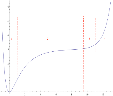
Inflation takes place in region 2 where the dynamics is completely dominated by the first negative exponential in (50), and so the inflationary potential can very well be approximated as:
| (51) |
The boarder between region 1 and 2 is given by an inflectionary point with which develops when the second negative exponential in (50) starts competing with the first one. The parameter becomes of the order unity and so inflation ends. On the other hand, region 3 is characterised by the fact that the positive exponential in (50) starts becoming important leading to . We are still in the slow-roll regime but the spectral index becomes larger than unity in contradiction with CMB observations. Hence we do not consider any inflationary dynamics in this region. Finally the boarder between region 3 and 4 is set by the violation of the slow-roll conditions. Further away in this final region fully dominated by the positive exponential, perturbation theory breaks down due to the fact that the K3 fibre modulus becomes extremely large while the 2-cycle which is the basis of the fibration shrinks to zero size.
This is a nice example of large field inflation since . Furthermore, all adjustable parameters enter only in the prefactor of the inflationary potential, making this model very predictive and leading to an interesting relation between and :
| (52) |
The prediction for the cosmological observables is and . The inflationary scale is fixed by the requirement of generating the observed density perturbations, and sets corresponding to GeV.
Contrary to ‘Blow-up inflation’, this mechanism does not suffer from the -problem in the sense that no corrections to arise at loop level. Being a large field model, loop corrections are suppressed by the size of the field and are naturally small. The -problem is absent because the supergravity potential being almost no-scale is not generic, while the arguments used regarding the -problem assume a generic Kähler potential. There is also a symmetry enhancement in the limit of infinite volume.
4.3 Axions as inflaton fields
As we have already pointed out, the action of an axion field enjoys a shift symmetry which is perturbatively exact. Hence no axion-dependent dimension 6 -suppressed operator of the form can arise, singling out the axion as a natural inflaton candidate in relation to this nice partial solution of the -problem.
4.3.1 Single axion
A typical axion potential is given by:
| (53) |
where denotes the axion decay constant which sets its coupling to gauge bosons:
| (54) |
In the case of -axions , where is an internal 4-cycle, the axion potential might be generated by a stringy instanton wrapping . As we have already seen, the superpotential for the LVS is with , and so the scalar potential in units of becomes (ignoring corrections):
| (55) |
We can therefore reproduce a potential of the form (53) with the scale given by:
| (56) |
The slow-roll parameters for the axion potential (53) look like:
| (57) |
| (58) |
showing how only if , but this is never the case. Thus we realise that the potential of a single axion is not flat enough to drive inflation.
4.3.2 Racetrack inflation
The ‘Racetrack inflation’ models were the first explicit examples of closed string inflation [15]. They were both realised in the context of the KKLT scenario with one and two Kähler moduli respectively. In the first scenario the single-field KKLT framework is modified by including a racetrack superpotential [44]:
| (59) |
The scalar potential has a saddle point in the direction of the axion component of . By a tuning of the parameters of order , the region close to the saddle point can be made flat enough to allow (topological eternal [45]) inflation. The main observational implications are a spectral index and negligible tensor modes ().
Very similar physical implications are obtained in the improved ‘Racetrack inflation’ scenario. In this case the Calabi-Yau manifold has two Kähler moduli and with Kähler and superpotential of the form:
| (60) |
In this case there are two axion-like fields and there is much less room to play with the parameters. However inflation is also obtained in one of the axionic directions. The amount of fine-tuning is similar to the single field case as well as all the physical implications. In particular the value of the spectral index fits perfectly well within the experimentally allowed window.
Both these scenarios were important to realise inflation in a concrete string model even if the amount of fine-tuning of the underlying parameters is significant.
4.3.3 N-flation
The first inflationary scenario based on more than one axion, say for definiteness of them, is the ‘N-flation’ model [21]. The total action takes the form:
| (61) |
The equations of motion imply that each axion evolves independently. However focusing on the collective motion of the axions we obtain:
| (62) |
which gives rise to the possibility to get and for if . Moreover one can get large tensor modes even if each single axion travels a sub-planckian distance in field space: .
The main obstacle against the realisation of such a multiple axion inflationary scenario is the need to fix all the real parts of the -moduli at an energy larger than the axion potential: . This is the only way to avoid the presence of dangerous steep directions along which the field would quickly roll down destroying the inflationary dynamics. However in general the non-perturbative effects used to generate the axion potential give also a mass to the 4-cycle moduli of the same order of magnitude: . For example focusing again on the LVS, . Thus one should try to fix all the ’s perturbatively, which is a hard task without invoking fine-tuning. Another issue is that one should check that these axions do not get eaten-up by any Green-Schwarz mechanism.
4.3.4 Axion monodromy
The first example of a single axion with a flat potential and has been provided by the ‘Axion monodromy’ model [23]. The key-ingredient to obtain a trans-planckian motion for a field like an axion which is periodic with period given by its decay constant: , is to use monodromy, i.e. studying how the axion behaves when it turns around a singularity.
In the case of -branes wrapping a 2-cycle of size , the action for the axion is:
| (63) |
At large , the potential can be approximated as , becoming linear in the canonically normalised inflaton . The -brane breaks the shift symmetry and gives a non-periodic contribution as . Thus undergoes a monodromy that ‘unwraps’ the axion circle. However appears also in the tree-level Kähler potential , and so it is not a good inflaton candidate due to the presence of higher order operators.
A better candidate is the -axion since it does not appear in . Wrapping an -brane around , the potential for the axion looks like:
| (64) |
Again at large , the potential can be approximated as , becoming linear in the canonically normalised inflaton. The inclusion of non-perturbative effects in the Kähler potential from an instanton wrapping gives rise to a cosine modulation:
| (65) |
One needs again to fix the real parts of the -moduli at a higher scale to avoid a possible destabilisation of the inflationary potential, which can be done using warping. The spectral index is and, due to a trans-planckian field range, , observable tensor modes with get produced. Moreover the cosine modulation gives ripples in the power-spectrum [46] and resonant non-gaussianities [47]. However this very promising inflationary model is missing a fully consistent compact example.
5 Open issues beyond inflation
There are several open challenges in string cosmology beyond deriving just closed moduli inflation. In this section we shall just briefly mention some of them:
- •
-
•
Study of finite-temperature corrections to the moduli potential from the thermal bath. In this way one finds a maximal temperature that sets an upper bound on the reheat temperature, , to avoid a decompactification limit. In the KKLT case GeV for TeV [48], while for the LVS case, GeV [49]. It would also be interesting to find a model where finite-temperature corrections generate a late epoch of thermal inflation [50] which might be needed to eliminate relics in the later Universe.
- •
-
•
Derivation of inflationary scenarios which allow TeV-scale supersymmetry solving the generic tension between cosmology and particle phenomenology [54]. The origin of this tension can be illustrated expressing the inflationary scale as and noticing that the scalar potential in the KKLT and LVS cases scale as:
(66) Thus for KKLT: while for LVS: . The requirement of generating the density perturbations, , generically sets , which implies TeV.
Two available solutions are:
-
1.
The volume can be used as the inflaton field [25]. In this way a high inflationary scale can be obtained by having small during inflation, while a low can be achieved for large at the end of inflation. Unfortunately this scenario requires fine-tuning.
-
2.
Some MSSM realisations via -branes at orbifold singularities can be sequestered from the bulk, resulting in a hierarchy between and which might be even of the order [55]. These models allow TeV for large .
-
1.
-
•
Study of multi-field inflationary dynamics that can provide alternative mechanisms [56, 57] to generate the density perturbations, which can lower the inflationary scale and give rise to large non-Gaussianities. Two interesting scenarios are:
- 1.
- 2.
References
References
- [1] F. Quevedo, Class. Quant. Grav. 19 (2002) 5721 [arXiv:hep-th/0210292]; R. Kallosh, Lect. Notes Phys. 738 (2008) 119 [arXiv:hep-th/0702059]; C. P. Burgess, PoS P2GC (2006) 008 [Class. Quant. Grav. 24 (2007) S795] [arXiv:0708.2865 [hep-th]]; L. McAllister and E. Silverstein, Gen. Rel. Grav. 40 (2008) 565 [arXiv:0710.2951 [hep-th]]; M. Cicoli, Fortsch. Phys. 58 (2010) 115 [arXiv:0907.0665 [hep-th]].
- [2] D. Lust et al, Nucl. Phys. B 808 (2009) 1 [arXiv:0807.3333 [hep-th]]; D. Lust et al, Nucl. Phys. B 828 (2010) 139 [arXiv:0908.0409 [hep-th]]; M. Cicoli et al, arXiv:1105.2107 [hep-th].
- [3] E. J. Copeland et al, Phys. Rev. D 49 (1994) 6410 [arXiv:astro-ph/9401011].
- [4] D. Baumann and L. McAllister, Phys. Rev. D 75 (2007) 123508 [arXiv:hep-th/0610285].
- [5] R. Kallosh and A. Linde, JCAP 0704 (2007) 017 [arXiv:0704.0647 [hep-th]].
- [6] N. Barnaby et al, JCAP 0504 (2005) 007 [arXiv:hep-th/0412040]; L. Kofman and P. Yi, Phys. Rev. D 72 (2005) 106001 [arXiv:hep-th/0507257]; D. Chialva et al, JHEP 0601 (2006) 014 [arXiv:hep-th/0508229].
- [7] D. R. Green, Phys. Rev. D 76 (2007) 103504 [arXiv:0707.3832 [hep-th]]; N. Barnaby et al, JCAP 0912 (2009) 021 [arXiv:0909.0503 [hep-th]]; M. Cicoli and A. Mazumdar, JCAP 1009 (2010) 025 [arXiv:1005.5076 [hep-th]]; M. Cicoli and A. Mazumdar Phys. Rev. D 83 (2011) 063527 [arXiv:1010.0941 [hep-th]].
- [8] M. B. Hindmarsh and T. W. B. Kibble, Rept. Prog. Phys. 58 (1995) 477 [arXiv:hep-ph/9411342].
- [9] G. R. Dvali and S. H. H. Tye, Phys. Lett. B 450 (1999) 72 [arXiv:hep-ph/9812483].
- [10] C. P. Burgess et al, JHEP 0107 (2001) 047 [arXiv:hep-th/0105204]; G. R. Dvali et al, arXiv:hep-th/0105203; C. Herdeiro et al, JHEP 0112 (2001) 027 [arXiv:hep-th/0110271]; C. P. Burgess et al, JHEP 0203 (2002) 052 [arXiv:hep-th/0111025]; S. Kachru et al, JCAP 0310 (2003) 013 [arXiv:hep-th/0308055]; H. Firouzjahi and S. H. H. Tye, Phys. Lett. B 584 (2004) 147 [arXiv:hep-th/0312020]; N. Iizuka and S. P. Trivedi, Phys. Rev. D 70 (2004) 043519 [arXiv:hep-th/0403203]; C. P. Burgess et al, JHEP 09 (2004) 033 [arXiv:hep-th/0403119].
- [11] D.H. Lyth, Phys. Rev. Lett. 78 (1997) 1861 [arXiv:hep-ph/9606387].
- [12] L. Verde, H. Peiris and R. Jimenez, JCAP 0601 (2006) 019 [arXiv:astro-ph/0506036].
- [13] J. Bock et al, arXiv:0805.4207 [astro-ph].
- [14] P. Binetruy and M. K. Gaillard, Phys. Rev. D 34, 3069 (1986); T. Banks et al, Phys. Rev. D 52, 3548 (1995) [arXiv:hep-th/9503114].
- [15] J. J. Blanco-Pillado et al, JHEP 0411 (2004) 063 [arXiv:hep-th/0406230]; J. J. Blanco-Pillado et al, JHEP 0609 (2006) 002 [arXiv:hep-th/0603129].
- [16] J. P. Conlon and F. Quevedo, JHEP 0601 (2006) 146 [arXiv:hep-th/0509012]; J. R. Bond et al, Phys. Rev. D 75 (2007) 123511 [arXiv:hep-th/0612197].
- [17] M. Cicoli, C. P. Burgess and F. Quevedo, JCAP 0903 (2009) 013 [arXiv:0808.0691 [hep-th]].
- [18] E. Silverstein and D. Tong, Phys. Rev. D 70, 103505 (2004) [arXiv:hep-th/0310221]; M. Alishahiha et al, Phys. Rev. D 70, 123505 (2004) [arXiv:hep-th/0404084]; K. Becker et al, Nucl. Phys. B 715, 349 (2005) [arXiv:hep-th/0501130].
- [19] S. Kachru et al, Phys. Rev. D 68, 046005 (2003) [arXiv:hep-th/0301240].
- [20] D. Baumann et al, JCAP 0801 (2008) 024 [arXiv:0706.0360 [hep-th]].
- [21] S. Dimopoulos et al, JCAP 0808, 003 (2008) [arXiv:hep-th/0507205].
- [22] T. W. Grimm, Phys. Rev. D 77 (2008) 126007 [arXiv:0710.3883 [hep-th]].
- [23] E. Silverstein and A. Westphal, Phys. Rev. D 78, 106003 (2008) [arXiv:0803.3085 [hep-th]]; L. McAllister et al, Phys. Rev. D 82 (2010) 046003 [arXiv:0808.0706 [hep-th]].
- [24] N. Kaloper, A. Lawrence and L. Sorbo, JCAP 1103 (2011) 023 [arXiv:1101.0026 [hep-th]].
- [25] J. P. Conlon et al, JCAP 0809 (2008) 011 [arXiv:0806.0809 [hep-th]].
- [26] A. Avgoustidis et al, Gen. Rel. Grav. 39 (2007) 1203 [arXiv:hep-th/0606031]; M. Badziak and M. Olechowski, JCAP 0807, 021 (2008) [arXiv:0802.1014 [hep-th]]; H. X. Yang and H. L. Ma, JCAP 0808 (2008) 024 [arXiv:0804.3653 [hep-th]].
- [27] S. B. Giddings et al, Phys. Rev. D 66 (2002) 106006 [arXiv:hep-th/0105097].
- [28] K. Becker, M. Becker, M. Haack, and J. Louis, JHEP 0206 (2002) 060 [arXiv:hep-th/0204254].
- [29] M. Berg, M. Haack, and B. Kors, JHEP 0511 (2005) 030 [arXiv:hep-th/0508043].
- [30] M. Berg, M. Haack and E. Pajer, JHEP 0709 (2007) 031 [arXiv:0704.0737 [hep-th]].
- [31] M. Cicoli, J. P. Conlon and F. Quevedo, JHEP 0801 (2008) 052 [arXiv:0708.1873 [hep-th]].
- [32] S. R. Coleman and E. Weinberg, Phys. Rev. D 7 (1973) 1888; S. Ferrara et al, Nucl. Phys. B 429 (1994) 589 [Erratum-ibid. B 433 (1995) 255] [arXiv:hep-th/9405188].
- [33] G. von Gersdorff and A. Hebecker, Phys. Lett. B 624 (2005) 270 [arXiv:hep-th/0507131].
- [34] J. P. Hsu and R. Kallosh, JHEP 0404 (2004) 042 [arXiv:hep-th/0402047].
- [35] L. Covi et al, JHEP 0806 (2008) 057 [arXiv:0804.1073 [hep-th]].
- [36] L. Covi et al, JHEP 0808 (2008) 055 [arXiv:0805.3290 [hep-th]].
- [37] R. Blumenhagen, S. Moster and E. Plauschinn, JHEP 0801 (2008) 058 [arXiv:0711.3389 [hep-th]].
- [38] V. Balasubramanian et al, JHEP 0503 (2005) 007 [arXiv:hep-th/0502058].
- [39] M. Cicoli, J. P. Conlon and F. Quevedo, JHEP 0810 (2008) 105 [arXiv:0805.1029 [hep-th]].
- [40] J. P. Conlon, F. Quevedo and K. Suruliz, JHEP 0508 (2005) 007 [arXiv:hep-th/0505076].
- [41] C. P. Burgess, R. Kallosh, and F. Quevedo, JHEP 0310 (2003) 056 [arXiv:hep-th/0309187].
- [42] S. L. Parameswaran and A. Westphal, JHEP 0610 (2006) 079 [arXiv:hep-th/0602253]; D. Cremades et al, JHEP 0705 (2007) 100 [arXiv:hep-th/0701154]; S. Krippendorf and F. Quevedo, JHEP 0911 (2009) 039 [arXiv:0901.0683 [hep-th]]. M. Cicoli et al, arXiv:1103.3705 [hep-th].
- [43] A. Saltman and E. Silverstein, JHEP 0411 (2004) 066 [arXiv:hep-th/0402135]; A. Westphal, JHEP 0703 (2007) 102 [arXiv:hep-th/0611332].
- [44] C. Escoda, M. Gomez-Reino and F. Quevedo, JHEP 0311 (2003) 065 [arXiv:hep-th/0307160].
- [45] A. D. Linde, Phys. Lett. B 327 (1994) 208 [arXiv:astro-ph/9402031]; A. Vilenkin, Phys. Rev. Lett. 72 (1994) 3137 [arXiv:hep-th/9402085].
- [46] R. Flauger et al, JCAP 1006, 009 (2010) [arXiv:0907.2916 [hep-th]].
- [47] S. Hannestad et al, JCAP 1006, 001 (2010) [arXiv:0912.3527 [hep-ph]].
- [48] W. Buchmuller et al, JCAP 0501 (2005) 004 [arXiv:hep-th/0411109]; W. Buchmuller et al, Nucl. Phys. B699 (2004) 292 [arXiv:hep-th/0404168].
- [49] L. Anguelova, V. Calo and M. Cicoli, JCAP 0910 (2009) 025 [arXiv:0904.0051 [hep-th]].
- [50] D. H. Lyth and E. D. Stewart, Phys. Rev. Lett. 75 (1995) 201 [arXiv:hep-ph/9502417]; D. H. Lyth and E. D. Stewart, Phys. Rev. D 53 (1996) 1784 [arXiv:hep-ph/9510204].
- [51] T. Barreiro et al, Phys. Rev. D 78, 063502 (2008) [arXiv:0712.2394 [hep-ph]].
- [52] J. P. Conlon and F. Quevedo, JCAP 0708 (2007) 019 [arXiv:0705.3460 [hep-ph]].
- [53] B. S. Acharya et al, JHEP 0806 (2008) 064 [arXiv:0804.0863 [hep-ph]].
- [54] R. Kallosh and A. Linde, JHEP 0412 (2004) 004 [arXiv:hep-th/0411011].
- [55] R. Blumenhagen et al, JHEP 0909 (2009) 007 [arXiv:0906.3297 [hep-th]].
- [56] D. H. Lyth and D. Wands, Phys. Lett. B 524 (2002) 5 [arXiv:hep-ph/0110002]; D. H. Lyth, JCAP 0511 (2005) 006 [arXiv:astro-ph/0510443]; K. Ichikawa et al, Phys. Rev. D 78 (2008) 023513 [arXiv:0802.4138 [astro-ph]].
- [57] G. Dvali et al, Phys. Rev. D 69 (2004) 023505 [arXiv:astro-ph/0303591]; G. Dvali et al, Phys. Rev. D 69 (2004) 083505 [arXiv:astro-ph/0305548]; L. Kofman, arXiv:astro-ph/0303614.
- [58] C. P. Burgess et al, JHEP 1008 (2010) 045 [arXiv:1005.4840 [hep-th]].
- [59] C. P. Burgess, M. Cicoli, M. Gomez-Reino, F. Quevedo, G. Tasinato and I. Zavala, in preparation.