Spontaneously Induced General Relativity:
Holographic Interior for Reissner-Nordstrom Exterior

Abstract

If general relativity is spontaneously induced, that is if the reciprocal Newton constant serves as a VEV, the electrically charged black hole limit is governed by a Davidson-Gurwich phase transition which occurs precisely at the would have been outer horizon. The transition profile which connects the exterior Reissner-Nordstrom solution with the novel interior is analytically derived. The inner core is characterized by a vanishing spatial volume and constant surface gravity, and in some respects, resembles a maximally stretched horizon. The Komar mass residing inside any concentric interior sphere is proportional to the surface area of that sphere, and consequently, is non-negative definite and furthermore non-singular at the origin. The Kruskal structure is recovered, admitting the exact Hawking imaginary time periodicity, but unconventionally, with the conic defect defused at the origin. The corresponding holographic entropy packing locally saturates the ’t Hooft-Susskind-Bousso holographic bound, thus making the core Nature’s ultimate information storage.

I Introduction

Bekenstein-Hawking area entropy HB , which plays a central role in black hole thermodynamics, has given rise to the speculative idea that no physical degrees of freedom reside within the interior of a black hole. Such an idea is theoretically backed by the fact that neither the Gibbons-Hawking GH Euclidean path integral derivation, nor the more locally oriented Wald’s Wald derivation, make actually use of the black hole interior. One may thus conclude that, as far as entropy packing is concerned, the interior of a black hole is apparently superfluous, so that the black hole degrees of freedom, whatever they are, live on or just above the outer horizon. The deal being one bit of information per a quarter of Planck area of the horizon surface bit . The apparent inconsistency between the horizon as a physical entity, the residence stretch of the black hole degrees of freedom, and as the mere point of no return for all in-falling matter, has ignited a well advertised debate in the physical society. The black hole area entropy formula has inspired the so-called holographic principle. The latter asserts that all of information contained in some region of space can be represented as a ’hologram’ on the boundary of that region. It furthermore puts a universal purely geometrical bound, saturated by Bekenstein-Hawking area entropy, on the amount of entropy stored within that region, namely

$$S\leq\frac{A}{4G}~{},$$ (1)

where $A$ denotes the area of the closed spacial boundary, $G$ is Newton’s constant, and $\hbar=c=k_{B}=1$. The holographic principle, primarily introduced by ’t Hooft tHooft , attempting to resolve the black hole information paradox, has been further developed by Susskind Susskind to deal with black hole complementarity, and has eventually acquired a covariant generalization by Bousso Bousso . The holographic principle is recently gaining a major theoretical support from the AdS/CFT duality AdsCFT .

It is commonly believed that general relativity is not necessarily the ultimate theory of gravity. If it is not the fundamental, but rather (say) a spontaneously induced theory of gravity, with $G^{-1}$ treated as a VEV, the black hole limit has been shown Essay to be governed by a phase transition which occurs precisely at the would have been event horizon. Recall that the idea of horizon phase transition PhaseTransition is not new (and in a similar category are black stars BlackStar and stringy fuzzballs fuzzballs ). Whereas the general relativistic exterior black hole solution is fully recovered, it serendipitously connects now, by means of a smooth self similar transition profile, with a novel holographic core. This core is characterized, among other things, by a vanishing spatial volume, a crucial feature for black hole physics. It is in this context of spontaneously induced general relativity that the first local realization of maximal entropy packing has been demonstrated DG . To be a bit more specific, sticking momentarily to spherical symmetry, it has been shown that associated with any inner sphere of circumferential radius $r$ is the total purely geometrical universal entropy

$$S(r)=\frac{\pi r^{2}}{G}~{},$$ (2)

which saturates the holographic bound layer by layer. The accompanying Komar mass Komar , as well as Weinberg’s material energy Weinberg , are notably non-singular, namely

$$M(r)=M(h)\frac{r^{2}}{h^{2}}~{},$$ (3)

where $M(h)$ denotes the overall mass calculated at $r=h$, and $A=\pi h^{2}$ is the horizon area. Such a Komar mass distribution appears to be intimately related to, and thus as fundamental as, the entropy distribution itself. In addition, the fact that the corresponding invariant spatial volume $V(r)\rightarrow 0$ for every $r\leq h$ can explain why the black hole entropy, unlike in any other macroscopic system, is not proportional to the volume of the system. Rather than envision bits of information evenly spread on the horizon surface, they may actually inhabit, universally and holographically in an onion-like manner, the entire black hole interior.

In this paper, by providing a holographic interior for the Reissner-Nordstrom exterior, we extend the Davidson-Gurwich analysisDG . Our paper is organized as follows. We begin by motivating and then introducing the action which governs the spontaneously induces general relativity, and derive the associated gravitational and scalar field equations (section II). These equations do not seem to admit a generic analytical solution, so we start by deriving their asymptotic behavior for the static spherically symmetric case, focusing on the deviation from the Reissner-Nordstrom background (section III). The asymptotic expansion is then used as a boundary condition for numerically plotting the various functions floating around, and to get a first glimpse into the characteristic phase transition which is developed at the would have been black hole horizon (section IV). At this stage, one can already appreciate the vanishing invariant volume of the novel interior core. Consequently, by systematically getting rid of the negligible terms in the field equations, we derive the approximate analytic solution of the core metric (section V). The in-out self-similar transition profile is analytically calculated (section VI), allowing us to finally fix the left over parameters of the inner solution by means of the mass $M$ and the elecric charge $Q$. Various aspects of the inner metric, such as vanishing volume, light cones, Kruskal structure, and singularity issues are discussed in section VII. Finally, owing to the recovery of the exact Hawking imaginary time periodicity (by defusing a conic singularity near the origin) and the emerging of a characteristic non-singular Komar mass function (section VIII), we re-formulate the holographic entropy packing, emphasizing its universal geometric structure (section IX).

II Action and Field equations

The simplest theory which accounts for the coupling of electromagnetism to spontaneously induced general relativity is given by the action

$${\cal I}=-\frac{1}{16\pi}\int\left(\phi R+V(\phi)+F^{\mu\nu}F_{\mu\nu}\right)\sqrt{-g}~{}d^{4}x~{}.$$ (4)

The role of the scalar potential is to allow the conformally coupled Brans-Dicke BD scalar field $\phi(x)$ to develop the vacuum expectation value (VEV)

$$\langle\phi\rangle=\frac{1}{G}~{}.$$ (5)

Several remarks are in order:

(i) The scalar field is kept electrically neutral, and furthermore does not couple directly to electromagnetism. This defines the Jordan frame, rather than the Einstein frame, to be the physical one. Our main conclusions turn out, however, to be frame independent.

(ii) On simplicity grounds, a kinetic scalar term has not been introduced. This, as we shall see, does not make the scalar field non-dynamical. Adding a kinetic term is always a viable option though, with minor effects on the inner metric.

(iii) The specific choice of the double well scalar potential

$$V(\phi)=\frac{3}{2a}\left(\phi-\frac{1}{G}\right)^{2}~{},$$ (6)

makes the theory fully equivalent to a simple $f(R)$ gravity f(R) theory, namely

$${\cal I}=-\frac{1}{16\pi}\int\left(\frac{1}{G}R-\frac{a}{6}R^{2}+F^{\mu\nu}F_{\mu\nu}\right)\sqrt{-g}~{}d^{4}x~{}.$$ (7)

In particular, stability $\acute{\text{a}}$ la Sotiriou-Faraoni stability is guaranteed by construction for $a>0$. The value of $a$ can be made as small as necessary to be compatible with Solar System tests.

Varying the action eq.(4) with respect to the three dynamical fields $g_{\mu\nu},A_{\mu},\phi$ leads respectively to the following equations of motion

$$\phi G_{\mu\nu}+\phi_{;\mu\nu}-g_{\mu\nu}\square\phi$$

$$\quad=\frac{V(\phi)}{2}g_{\mu\nu}-2F_{\mu\alpha}F_{\nu\beta}g^{\alpha\beta}+\frac{F^{2}}{2}g_{\mu\nu}~{},$$ (8)

$$F^{\mu\nu}_{~{};\nu}=0~{},$$ (9)

$$R+\frac{dV(\phi)}{d\phi}=0~{}.$$ (10)

By tracing the gravitational field eqs.(8), and then substituting the resulting Ricci scalar into eq.(10), one can extract the associated Klein Gordon equation

$$\square\phi=\frac{1}{3}\left(\phi\frac{dV(\phi)}{d\phi}-2V(\phi)\right)\equiv\frac{dV_{eff}(\phi)}{d\phi}~{}.$$ (11)

The evolution of the scalar field is thus governed by the effective potential

$$V_{eff}(\phi)=\frac{1}{2aG}\left(\phi-\frac{1}{G}\right)^{2}+const~{}.$$ (12)

The similarity between the two potentials $V(\phi)$ and $V_{eff}(\phi)$ is not generic.

At this stage, our interest lies with the static spherically symmetric case, with the corresponding line element taking the conventional form

$$ds^{2}=-e^{\nu(r)}dt^{2}+e^{\lambda(r)}dr^{2}+r^{2}d\Omega^{2}~{}.$$ (13)

The only non-vanishing entries of the electromagnetic tensor are

$$F_{tr}=-F_{rt}=E(r)~{}.$$ (14)

First, we solve the associated Maxwell equation

$$E^{\prime}(r)+\left(\frac{2}{r}-\frac{\nu^{\prime}(r)+\lambda^{\prime}(r)}{2}\right)E(r)=0~{},$$ (15)

whose straight forward solution is given by

$$\ E(r)=\frac{Q}{r^{2}}e^{\frac{\lambda(r)+\nu(r)}{2}}~{},$$ (16)

with $Q$ denoting the electric charge. Next, we substitute eq.(16) into the three independent gravitational and scalar field equations, which can then be reorganized in the master form

$$\phi^{\prime\prime}-\frac{1}{2}\left(\nu^{\prime}+\lambda^{\prime}\right)\left(\phi^{\prime}+\frac{2}{r}\phi\right)=0~{},$$ (17)

$$\phi^{\prime\prime}+\frac{1}{2}\left(\nu^{\prime}-\lambda^{\prime}\right)\left(\phi^{\prime}-\frac{2}{r}\phi\right)-\frac{2}{r^{2}}\left(1-e^{\lambda}\right)\phi$$

$$\quad\quad=\frac{3e^{\lambda}}{2a}\left(\phi-\frac{1}{G}\right)\left(\phi+\frac{1}{3G}\right)+2e^{\lambda}\frac{Q^{2}}{r^{4}}~{},$$ (18)

$$\phi^{\prime\prime}+\left(\frac{2}{r}+\frac{\nu^{\prime}-\lambda^{\prime}}{2}\right)\phi^{\prime}=\frac{e^{\lambda}}{aG}\left(\phi-\frac{1}{G}\right)~{}.$$ (19)

One can easily verify that associated with the vacuum solution $\displaystyle{\phi(r)=\frac{1}{G}}$ is the Reissner Nordstrom (RN) black hole metric

$$e^{\nu(r)}=e^{-\lambda(r)}=1-\frac{2GM}{r}+\frac{GQ^{2}}{r^{2}}~{}.$$ (20)

However, unlike in general relativity, the Reissner-Nordstrom solution, which we hereby tag with some $\epsilon=0$, is now accompanied by a general class of asymptotically flat $\epsilon\neq 0$ solutions. In this language, our paper is mainly devoted to the unfamiliar physics encountered at the $\epsilon\rightarrow 0$ limit.

III Asymptotic behavior

A general analytic solution of our field equations is still at large. Alternatively, we adopt the strategy to use an asymptotically flat perturbation around the RN solution as a boundary condition for the numerical solution of the field equations. Needless to say, the numeric solution by itself is not our final goal, but the resulting graphs will give us the first clue regarding the structure of the phase transition awaiting ahead. Consider thus a perturbative solution of the general form

$$\phi(r)=\frac{1}{G}\left(1+s\phi_{1}(r)\right)~{},$$ (21)

$$\lambda(r)=-\log\left(1-\frac{2GM}{r}+\frac{GQ^{2}}{r^{2}}+sL_{1}(r)\right)~{},$$ (22)

$$\nu(r)=\log\left(1-\frac{2GM}{r}+\frac{GQ^{2}}{r^{2}}+sN_{1}(r)\right)~{},$$ (23)

where the constant $s$, which can be interpreted as the scalar charge, serves as our small expansion parameter. Naively, one may expect general relativity to be fully recovered at the limit $s\rightarrow 0$, but as we are about to see, this is not necessarily the case. Of particular interest for us is the decoupled linear differential equation

$$\left(1-\frac{2GM}{r}+\frac{GQ^{2}}{r^{2}}\right)\phi_{1}^{\prime\prime}(r)$$

$$\quad+\frac{2}{r}\left(1-\frac{GM}{r}\right)\phi_{1}^{\prime}(r)-\frac{1}{aG}\phi_{1}(r)=0~{},$$ (24)

which quantifies the deviation $s\phi_{1}(r)$ from general relativity. Unfortunately, even this equation is not that cooperative. At large $r$, however, which is equivalent to neglecting $M$ and $Q$, one gets rid of the diverging term to stay with the converging Yukawa tail $\displaystyle{\sim\frac{1}{r}e^{-\frac{r}{\sqrt{aG}}}}$. Consequently, once $M$ and $Q$ are re-introduced, we expect the solution to be of the form

$$\phi_{1}(r)=\frac{f(r)}{r}e^{-\frac{r}{\sqrt{aG}}}~{}.$$ (25)

Clearly, the equation for $f(r)$ is still quite complicated, but it becomes manageable upon keeping only the leading terms at large $r$, that is

$$\sqrt{aG}f^{\prime\prime}(r)-2f^{\prime}(r)-\frac{2GM}{\sqrt{aG}r}f(r)\simeq 0~{}.$$ (26)

The solution of this equation involves the Hypergeometric and the so-called MeijerG functions. It so happens, however, that both these functions exhibit identical divergent behavior. In turn, one can always find a converging linear combination, with the latter being proportional to $\displaystyle{r^{-\frac{GM}{\sqrt{aG}}}}$. To be more specific,

$$\phi_{1}(r)\simeq\frac{e^{-\frac{r}{\sqrt{aG}}}}{r^{1+\frac{GM}{\sqrt{aG}}}}~{}.$$ (27)

With this in hands, we proceed to the linear differential equation for $L_{1}(r)$, namely

$$L_{1}(r)+rL_{1}^{\prime}(r)$$

$$=-\frac{G}{r}\left(Q^{2}-Mr\right)\phi_{1}^{\prime}(r)+\left(\frac{GQ^{2}}{r^{2}}-\frac{r^{2}}{aG}\right)\phi_{1}(r)~{}.$$ (28)

The solution of this equation is a sum of several Gamma functions which, at the large $r$ limit, is well approximated by the expression

$$L_{1}(r)\simeq\frac{1}{\sqrt{aG}}\frac{e^{-\frac{r}{\sqrt{aG}}}}{r^{\frac{GM}{\sqrt{aG}}}}~{}.$$ (29)

By the same token, one can also calculate

$$N_{1}(r)\simeq-\frac{e^{-\frac{r}{\sqrt{aG}}}}{r^{1+\frac{GM}{\sqrt{aG}}}}~{}.$$ (30)

IV Preliminary numerical insight

On pedagogical grounds, to have a glimpse at the new physics offered by spontaneously induced general relativity, we first plot numerical graphs of the various functions involved. Starting at some large enough distance

$$r_{max}>>GM,\sqrt{G}Q,\sqrt{aG}~{},$$ (31)

where the Reissner Nordstrom metric components and the inverse Newton constant are supplemented by the perturbations eqs.(27,29,30), we run a full numerical calculation which produces Figs.(1,2,3), respectively. We do it for a positive scalar charge $s>0$, and focus our attention on the limit $s\rightarrow+0$. The dashed lines in these graphs depict the underlying Reissner-Nordstrom solution.

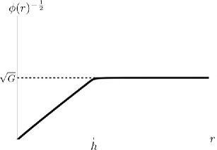
Figure 1: A generic scalar field configuration. As $s\rightarrow+0$, general relativity is recovered at the exterior region, but is spontaneously violated in the inner core.

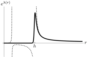
Figure 2: A generic $e^{\lambda(r)}$ plot. Whereas the exterior RN is recovered at the $s\rightarrow+0$ limit, the overall configuration conceptually differs from the full $s=0$ RN solution (dashed line).

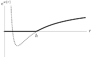
Figure 3: A generic $e^{\nu(r)}$ plot. Whereas the exterior RN is recovered at the $s\rightarrow+0$ limit, the overall configuration conceptually differs from the full $s=0$ RN solution (dashed line).

Naively, one would expect perhaps a full recovery of general relativity at the $s\rightarrow 0$ limit, but can already suspect the appearance of a phase transition near the would have been outer horizon, at

$$h=GM+\sqrt{G^{2}M^{2}-GQ^{2}}~{}.$$ (32)

Serendipitously, representing a ’level crossing’ effect (soon to be clarified), the limit $s\rightarrow+0$ does not reproduce the $s=0$ solution. While the exterior Reissner Nordstrom solution is recovered, which is indeed an important feature by itself, it now connects with a novel interior core. This new interior solution differs conceptually from the Reissner Nordstrom interior by three characteristic features, namely

1. No $t\longleftrightarrow r$ signature flip,

2. Drastically suppressed $e^{\nu(r),\lambda(r)}$, and

3. Locally varying effective Newton constant.

Following the preliminary numerical insight, we now proceed to uncover the geometry/physics of the inner core, and reveal the analytic structure of the phase transition profile.

V A novel core

The key feature now is the fact that $0<e^{\lambda(r)}\ll 1$ in the entire inner core. A closer numerical inspection reveals that all terms in the field equations eqs.(17,18,19) which are proportional to $e^{\lambda(r)}$ are practically negligible relative to the other terms. In particular, the negligible pieces include the scalar potential terms and the electromagnetic energy momentum contributions, thereby indicating a universal inner structure. The field equations take then the slimmer form

$$\phi^{\prime\prime}-\frac{\nu^{\prime}+\lambda^{\prime}}{2}\left(\phi^{\prime}+\frac{2}{r}\phi\right)=0~{},$$ (33)

$$\phi^{\prime\prime}+\frac{\nu^{\prime}-\lambda^{\prime}}{2}\left(\phi^{\prime}-\frac{2}{r}\phi\right)-\frac{2}{r^{2}}\left(1-\kappa e^{\lambda}\right)\phi=0~{},$$ (34)

$$\phi^{\prime\prime}+\left(\frac{2}{r}+\frac{\nu^{\prime}-\lambda^{\prime}}{2}\right)\phi^{\prime}=0~{}.$$ (35)

Strictly for the current approximation $\kappa=0$, but by introducing $\kappa$ we reserve the option of searching for the roots of the transition profile already within the $\kappa=1$ framework which corresponds to plain (insensitive to the scalar potential) $\phi R$ gravity. Switching $\kappa$ off and on is demonstrated in Fig.4.

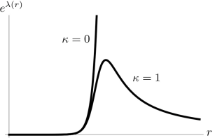
Figure 4: The suppression of $e^{\lambda(r)}$ in the inner core is fully captured by the $\kappa=0$ approximation. $\phi R$ gravity, switched on by $\kappa=1$, already exhibits the transition profile.

The above set of scale invariant equations admit an exact analytic solution given by

$$e^{\nu(r)}=\alpha\left(\frac{r}{h}\right)^{\frac{6}{\epsilon}-4}~{},$$

$$e^{\lambda(r)}=\beta\left(\frac{r}{h}\right)^{\frac{6}{\epsilon}-6+2\epsilon}~{},$$ (36)

$$\phi(r)=\gamma\left(\frac{r}{h}\right)^{-2+\epsilon}~{}.$$

This general solution is governed by a constant of integration $\epsilon\neq 0$. The self consistency of the approximation for all $r<h$ further requires $0<\epsilon\ll 1$. The scale $h$, however, marking the radius of the core (where $r/h$ ceases to be a fraction), is fictitious at this stage, and can be absorbed by re-defining the coefficients $\alpha,\beta,\gamma$. This is a consequence of the fact that eqs.(36) are scale invariant. It remains to be seen what actually fixes the small value of $\epsilon$, removes the arbitrariness of $\alpha,\beta,\gamma$ (in particular $\displaystyle{\gamma\rightarrow\frac{1}{G}}$, as suggested by Fig.1 on matching grounds), and furthermore turns the scale $h$ into the physical quantity defined by eq.(32). At any rate, following our analysis so far, one may rightly suspect an intriguing correlation between the $\epsilon\rightarrow+0$ limit which characterizes the short distance physics, and the $s\rightarrow+0$ limit relevant for the large distance physics.

VI Phase transition

Focus attention now in the neighborhood of $r=h$, where $e^{\lambda(r)}$ acquires its maximum value. We already know, based on numerical evidence (running Fig.4 for a variety of small $\epsilon$ values, that $e^{\lambda(h)}\sim\epsilon^{-1}$, and estimate the width of the transition area to be $\Gamma\sim\epsilon$. One may even suspects a universal self similar transition profile.

We probe the transition at the approximation where

$$e^{\lambda(r)}\left(\phi(r)-\frac{1}{G}\right)\simeq 0~{}.$$ (37)

Just inside, it is the $e^{\lambda(r)}$ factor which is highly suppressed, whereas for $r\geq h$ a similar suppression role is played by $\left(\phi(r)-\frac{1}{G}\right)$. The approximate eq.(35) stays then valid at the transition region as well, and upon a first integration, gives rise to the (negative) conserved quantity

$$\phi^{\prime}(r)r^{2}e^{\frac{\lambda(r)-\nu(r)}{2}}\simeq C~{}.$$ (38)

With eq.(38) incorporated, setting $r\simeq h$ and $\displaystyle{\phi(r)\simeq\frac{1}{G}}$ when appropriate, and neglecting relatively small terms, the two remaining recast field equations read

$$\nu^{\prime}-\lambda^{\prime}\simeq\frac{2}{h}\left(1-\frac{GQ^{2}}{h^{2}}\right)e^{\lambda}~{},$$ (39)

$$\nu^{\prime}+\lambda^{\prime}\simeq-\frac{2}{h}\left(1-\frac{GQ^{2}}{h^{2}}\right)\frac{e^{\lambda}}{1+\frac{2h}{GC}e^{\frac{\nu-\lambda}{2}}}~{}.$$ (40)

We find it useful to introduce

$$\sigma(r)=\frac{\lambda(r)-\nu(r)}{2}~{},$$ (41)

transforming the above pair of equations into

$$\sigma^{\prime}(r)=-\frac{1}{h}e^{\lambda(r)}\left(1-\frac{GQ^{2}}{h^{2}}\right)$$ (42)

$$\frac{\sigma^{\prime\prime}(r)}{\sigma^{\prime}(r)}-\sigma^{\prime}(r)=\frac{\sigma^{\prime}(r)e^{\sigma(r)}}{\frac{2h}{CG}+e^{\sigma(r)}}$$ (43)

Two successive integrations bring us then to the inverse solution $r(\sigma)$

$$r-\bar{r}=-\frac{CG}{2p}\left(e^{-\sigma(r)}-\frac{CG}{2h}\log\left(-\frac{2h}{CG}e^{-\sigma(r)}-1\right)\right)~{},$$ (44)

with two constants of integration $p$ and ${\bar{r}}$ floating around. Substituting back into eqs.(39,40), we finally arrive at the parametric solution

$$e^{\nu(r)}=-\frac{pe^{-\sigma(r)}}{1-\frac{GQ^{2}}{h^{2}}}\left(\frac{2h}{CG}+e^{\sigma(r)}\right)~{},$$ (45)

$$e^{\lambda(r)}=-\frac{pe^{\sigma(r)}}{1-\frac{GQ^{2}}{h^{2}}}\left(\frac{2h}{CG}+e^{\sigma(r)}\right)~{},$$ (46)

which we now attempt to connect with the approximate solutions for the exterior and the interior regimes. To do so, it is convenient to introduce a dimensionless variable

$$x=-\frac{2h}{CG}e^{-\sigma(r)}~{},$$ (47)

so that

$$r-\bar{r}=\frac{h}{p}\left(\frac{CG}{2h}\right)^{2}\left(x+\log(x-1)\right)~{},$$

$$e^{\nu(r)}=-\frac{p}{1-\frac{GQ^{2}}{h^{2}}}(1-x)~{}.$$ (48)

$$e^{\lambda(r)}=-\frac{p\left(\frac{2h}{CG}\right)^{2}}{1-\frac{GQ^{2}}{h^{2}}}\left(\frac{1-x}{x^{2}}\right)~{},$$

1. Matching with the Exterior

In the exterior, let $\displaystyle{x=\frac{1}{\delta}}$ for $0<\delta\ll 1$, hence

$$r-\bar{r}\simeq\frac{C^{2}G^{2}}{4ph}\frac{1}{\delta}~{},$$

$$e^{\nu(r)}\simeq\frac{p}{1-\frac{GQ^{2}}{h^{2}}}\frac{1}{\delta}\simeq\frac{r-\bar{r}}{\frac{C^{2}G^{2}}{4p^{2}h}\left(1-\frac{GQ^{2}}{h^{2}}\right)}~{},$$ (49)

$$e^{\lambda(r)}\simeq\frac{p\left(\frac{2h}{CG}\right)^{2}}{1-\frac{GQ^{2}}{h^{2}}}\delta\simeq\frac{h}{\left(1-\frac{GQ^{2}}{h^{2}}\right)\left(r-\bar{r}\right)}~{}.$$

This can be immediately recognized as the leading expansion terms just outside the Reissner Nordstrom outer horizon. In turn, up to first order corrections, we identify

$${\bar{r}}=h~{},$$ (50)

$$\displaystyle{\frac{p}{C^{2}}=\frac{G^{2}}{4h^{2}p}\left(1-\frac{GQ^{2}}{h^{2}}\right)^{2}~{}.}$$ (51)

2. Matching with the Interior

In the interior, let $x=1+\delta$ for $0<\delta\ll 1$, so that $\displaystyle{r-h\simeq\frac{C^{2}G^{2}}{4ph}\log\delta}$. Although $\log\delta$ is large, $\displaystyle{\frac{C^{2}G^{2}}{4ph^{2}}\log\delta}$ may still be small. In which case,

$$\frac{r}{h}=\delta^{\frac{C^{2}G^{2}}{4ph^{2}}}~{},$$

$$e^{\nu(r)}\simeq\frac{p}{1-\frac{GQ^{2}}{h^{2}}}\delta\simeq\frac{p}{1-\frac{GQ^{2}}{h^{2}}}\left(\frac{r}{h}\right)^{\frac{4ph^{2}}{C^{2}G^{2}}}~{},$$ (52)

$$e^{\lambda(r)}\simeq\frac{p\frac{4h^{2}}{C^{2}G^{2}}}{1-\frac{GQ^{2}}{h^{2}}}\delta\simeq\frac{p\frac{4h^{2}}{C^{2}G^{2}}}{1-\frac{GQ^{2}}{h^{2}}}\left(\frac{r}{h}\right)^{\frac{4ph^{2}}{C^{2}G^{2}}}~{}.$$

This set is nothing but the previously derived eqs.(36) provided we make the identification

$$\frac{\epsilon}{6}=\frac{p}{\left(1-\frac{GQ^{2}}{h^{2}}\right)^{2}}~{}.$$ (53)

We can now furthermore fix the otherwise arbitrary coefficients $\alpha,\beta,\gamma$ which enter the core metric

$$\alpha(\epsilon)=\frac{1}{\beta(\epsilon)}=\left(1-\frac{GQ^{2}}{h^{2}}\right)\frac{\epsilon}{6}~{},\quad\gamma(\epsilon)=\frac{1}{G}~{}.$$ (54)

3. Self similar transition profile

The maximum of $e^{\lambda(r)}$, serving as the characteristic cut-off of spontaneously induced general relativity, occurs for $\displaystyle{e^{-\sigma}=-\frac{CG}{h}}$, and takes the value

$$e^{\lambda}_{max}=\frac{3}{2\epsilon\left(1-\frac{GQ^{2}}{h^{2}}\right)}~{}.$$ (55)

The typical width $\Gamma$, where $e^{\lambda(r)}$ drops to half its maximal size, is given by

$$\Gamma\simeq\frac{\epsilon}{3}h~{},$$ (56)

such that $e^{\lambda}_{max}\Gamma$ stays $\epsilon$-independent. These features are demonstrated in Fig.5 for a variety of $\epsilon$ values (the dashed line represents the $\epsilon\rightarrow+0$ limit).

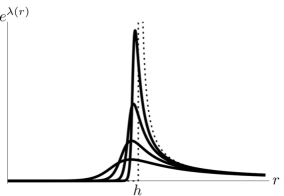
Figure 5: The in-out transition profile is plotted for a decreasing series of $\epsilon$ values. The phase transition into the exterior Reissner Nordstrom solution (dashed line) occurs as $\epsilon\rightarrow+0$.

Owing to the fact that its roots are located in the underlying $\phi R$ gravity, the transition profile turns out to be insensitive to the terms involving the scalar potential, and exhibits a remarkable self similarity feature. This is expressed by the fact that $\epsilon\rightarrow k\epsilon$ only causes scale changes

$$e^{\lambda}\rightarrow k^{-1}e^{\lambda}~{},$$ (57)

$$r-h\rightarrow k(r-h)~{}.$$ (58)

4. The $\epsilon\longleftrightarrow s$ interplay

$\epsilon$ parametrizes the short distance geometry, whereas the scalar charge $s$ parametrizes the long distance perturbation around the Reissner Nordstrom background. The remarkable correlation between the small-$\epsilon$ and the small-$s$ limits has already been qualitatively established, but it seems impossible to derive the exact $\epsilon(s)$ relation, and and at this stage, has only been obtained numerically. This can be done e.g. by plotting $\frac{12}{r}\left(\nu^{\prime}(r)+\lambda^{\prime}(r)\right)\simeq\epsilon$ at short distances, or alternatively by extracting $(e^{\lambda}_{max})^{-1}\sim\epsilon$ at the transition region.

First, one can numerically verify that $\epsilon(s)$ is practically $a$-independent, at least for large enough $a$’s. Thus, holding $a$ fixed, we then plot $\epsilon(s)$ for various values of $M$ (and momentarily keep $Q=0$). The results are summarized in Fig.6.

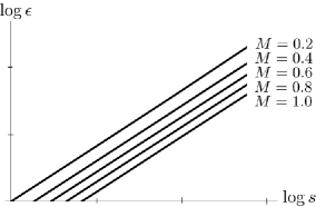
Figure 6: The $\epsilon\longleftrightarrow s$ interplay: The linearity of $\epsilon(s)$ is demonstrated for various values of $M$ (in units of $\sqrt{G/a}$).

From the slope we deduce that, for large $a$, $\epsilon$ is proportional to $s$, and that the proportionality factor is $M$-dependent. Taking into account the structure of the $s$ term which enters the approximation eq.(27), and invoking continuity arguments (next order necessarily included) at $r\simeq h$, we elegantly fit the numerical graphs by the empirical formula

$$\epsilon\simeq\frac{4e^{-\frac{h}{\sqrt{aG}}}s}{\left(1-\frac{GQ^{2}}{h^{2}}\right)h^{1+\frac{GM}{\sqrt{aG}}}}~{}.$$ (59)

VII Core geometry

Altogether, the core metric is well approximated by

$$ds^{2}_{in}\simeq-\alpha(\epsilon)\left(\frac{r}{h}\right)^{\frac{6}{\epsilon}-4}dt^{2}+\frac{1}{\alpha(\epsilon)}\left(\frac{r}{h}\right)^{\frac{6}{\epsilon}-6+2\epsilon}dr^{2}+r^{2}d\Omega^{2}~{},$$ (60)

where $\alpha(\epsilon)$ is given explicitly by eq.(54). This metric is accompanied by the associated scalar field

$$\phi(r)\simeq\frac{1}{G}\left(\frac{r}{h}\right)^{-2+\epsilon}~{}.$$ (61)

As $\epsilon\rightarrow+0$, the metric connects with the perturbed exterior Reissner Nordstrom spacetime, and the scalar field approaches its general relativistic VEV.

1. Vanishing volume

The first geometrical quantity to calculate is the invariant spatial volume $V(r)$ associated with a sphere of circumferential radius $r$. Doing it in the interior core, one approaches a vanishingly small volume at the $\epsilon\rightarrow+0$ limit, namely

$$V(r)=4\pi\int_{0}^{r}e^{\frac{1}{2}\lambda(r)}r^{2}~{}dr$$

$$\quad\simeq\sqrt{\frac{6\epsilon}{1-\frac{GQ^{2}}{h^{2}}}}\left(\frac{r}{h}\right)^{\frac{3}{\epsilon}}\frac{4\pi}{3}h^{3}~{}.$$ (62)

This is to be fully contrasted with the corresponding finite surface area

$$A(r)=4\pi r^{2}~{}.$$ (63)

The $V(r)$ plot, depicted in Fig.7, gives us a simple answer why is the black hole volume physically irrelevant (unlike in any other system, the black hole entropy is proportional to the horizon surface area).

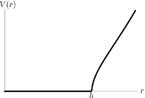
Figure 7: The invariant volume $V(r)$: Every inner concentric sphere of finite surface area $4\pi r^{2}$ exhibits a vanishingly small volume.

2. Light cone structure

Radial null geodesics at $r=h+\delta r$, just outside the would have been horizon, obey

$$\frac{dr}{dt}=\pm\left(1-\frac{GQ^{2}}{h^{2}}\right)\frac{\delta r}{h}~{}.$$ (64)

Inside the core, the formula transforms into

$$\frac{dr}{dt}=\pm\left(1-\frac{GQ^{2}}{h^{2}}\right)\frac{\epsilon r}{6h}~{},$$ (65)

where the exact role played by $\delta r$ in eq.(64) is being taken by $\frac{1}{6}\epsilon r$ in eq.(65). In particular, as far as an observer at asymptotic distances is concerned, a light ray sent from some $r_{0}<h$ inwards will never reach the origin even for a finite $\epsilon$, as can be seen from

$$r(t)=r_{0}e^{-t/\tilde{t}},\quad\tilde{t}=\frac{6h}{\epsilon\left(1-\frac{GQ^{2}}{h^{2}}\right)}~{}.$$ (66)

In other words, the entire core resembles a ’near horizon’ territory, and as $\epsilon\rightarrow+0$, it looks from the outside as an apparently ’frozen world’ Paddy . In many respects, the role played by the outer Reissner Nordstrom event horizon gets now shifted to the origin.

3. Constant surface gravity

To get a deeper clue about what is going on, we calculate the surface gravity function

$$\kappa(r)=\frac{\nu^{\prime}(r)}{2}e^{\frac{\nu(r)-\lambda(r)}{2}}$$ (67)

inside the core, and find

$$\kappa(r)\simeq\left(1-\frac{2}{3}\epsilon\right)\frac{1-\frac{GQ^{2}}{h^{2}}}{2h}\left(\frac{h}{r}\right)^{\epsilon}\rightarrow\kappa~{}.$$ (68)

Not only do we face a constant surface gravity core, all the way from $r\leq h$ to the origin at $r=0$, but its value is immediately identified as $2\pi$ the Hawking temperature

$$\boxed{\kappa=\frac{1}{2h}\left(1-\frac{GQ^{2}}{h^{2}}\right)}~{}.$$ (69)

This will certainly have far reaching consequences (soon to be revealed) on the Komar mass and the associated thermodynamics.

4. Singularity issues?

When approaching the origin, it is convenient to invoke the proper length coordinate

$$\eta(r)=\frac{h\left(\frac{r}{h}\right)^{-2+\frac{3}{\epsilon}+\epsilon}}{\left(\frac{3}{\epsilon}-2+\epsilon\right)\sqrt{\left(1-\frac{GQ^{2}}{h^{2}}\right)\frac{\epsilon}{6}}}~{},$$ (70)

and expand the inner metric, up to ${\cal O}(\epsilon)$ pieces, to expose the Rindler structure of the $R_{2}$ sub-metric

$$ds_{in}^{2}\simeq-\kappa^{2}\eta^{2}dt^{2}+d\eta^{2}+\left(\frac{3\kappa\eta^{2}}{\epsilon h}\right)^{\frac{3}{\epsilon}}h^{2}d\Omega^{2}~{}.$$ (71)

The recovery the exact Hawking’s imaginary time periodicity, which first of all reassures the accuracy of the transition profile eq.(VI), is regarded as the anchor connecting us to black hole thermodynamics. Notice, however, that unlike in the original Reissner Nordstrom case, the Euclidean origin corresponds now to the center of spherical symmetry $r=0$ rather than to $r=h$.

A word of caution is in order. Inside the core, the the various scalars are well approximated by

$$R=-\frac{2}{r(\eta)^{2}}~{},$$ (72)

$$R^{\mu\nu}R_{\mu\nu}\simeq\frac{8\epsilon^{2}}{9\eta^{4}}\left(1-\frac{GQ^{2}}{h^{2}}\right)^{2}+\left[\frac{2}{r^{4}(\eta)}\right]~{},$$ (73)

$$R^{\mu\nu\lambda\sigma}R_{\mu\nu\lambda\sigma}\simeq\frac{16\epsilon^{2}}{9\eta^{4}}\left(1-\frac{GQ^{2}}{h^{2}}\right)^{2}+\left[\frac{4}{r^{4}(\eta)}\right]~{},$$ (74)

where the square parentheses $\left[...\right]$ denote relatively small terms which survive the $\epsilon\rightarrow 0$ limit. Reflecting the $\displaystyle{\frac{\epsilon}{\eta^{2}}}$ ratio, the singularity analysis bifurcates:

(i) Clearly, for any finite $\eta$, as small as desired, the limit $\epsilon\rightarrow 0$ is regular. The Rindler sub-metric gets then multiplied by a 2-sphere of constant radius $h$, and consistently, the Kretschmann curvature approaches the Reissner Nordstrom horizon value of $\displaystyle{\frac{4}{h^{4}}}$.

(ii) However, for any finite $\epsilon$, as small as desired, the limit $\eta\rightarrow 0$ is singular. Whereas the pseudo-horizon does provide some protection from the singularity (e.g. it takes an infinite amount of time for light from the singularity to reach any external observer), an observer willing to wait long enough will see unbounded high curvature. Such a behavior is far worse than that of the Reissner Nordstrom solution, and constitutes a severe problem. It may be that a more complicated Lagrangian could alleviate this behavior, or else that quantum effects could eventually cure it.

The point is, however, that the parameter $\epsilon$ and the coordinate $\eta$ cannot really be treated on the same footing. Any given metric must first of all be specified by its parameters, and only then can it serve the whole range of coordinates. In turn, the right order is to first let $\epsilon\rightarrow 0$, and only then approach the $\eta\rightarrow 0$ origin. In other words, using momentarily a two variable language, $\epsilon$ must tend to zero faster than $\eta^{2}$ (we return to this point in the Kruskal analysis). This argument is supposed to solve the above dilemma by choosing the first option.

5. Kruskal structure at the origin

Another view on the geometry surrounding the origin is provided by means of the Kruskal-Szekeres coordinate transformation

$$u=f(r)\cosh\omega t~{},~{}v=f(r)\sinh\omega t~{},$$ (75)

which by choosing $\displaystyle{\frac{f^{\prime}(r)}{\omega f(r)}=e^{\frac{\lambda(r)-\nu(r)}{2}}}$ gives rise to a metric of the form

$$ds_{in}^{2}=K^{2}(r)\left(-dv^{2}+du^{2}\right)+r^{2}d\Omega^{2}~{}.$$ (76)

In our case, we find

$$\log f(r)\simeq\frac{6\omega h}{\left(1-\frac{GQ^{2}}{h^{2}}\right)}\frac{\left(\frac{r}{h}\right)^{\epsilon}}{\epsilon^{2}}~{},$$ (77)

and the crucial point has to do with the $\epsilon$-expansion

$$\left(\frac{r}{h}\right)^{\epsilon}=1+\epsilon\log\frac{r}{h}+\frac{1}{2}\left(\epsilon\log\frac{r}{h}\right)^{2}+...~{}.$$ (78)

As was emphasized earlier, a small parameter and a small coordinate cannot be treated on equal footing. The parameter $\epsilon$ which specifies the metric must tend to zero faster than any function of the coordinates, say $\left(\log\frac{r}{h}\right)^{-1}$ in this case. The corresponding Kruskal scale function $K(r)$ is then given by

$$K(r)\simeq\left(\frac{r}{h}\right)^{\displaystyle{\frac{3}{\epsilon}\left(1-\frac{2\omega h}{1-\frac{GQ^{2}}{h^{2}}}\right)}}~{},$$ (79)

which consistently singles out the Hawking imaginary time periodicity eq.(69) on the grounds of defusing the conic singularity at the origin.

5. Frame independence

Although the Jordan frame is the physical one in the hereby discussed theory, the Einstein frame is still of interest. In 4-dimensions, the transition is established by substituting

$$g_{\mu\nu}=\phi^{-1}\bar{g}_{\mu\nu}~{}.$$ (80)

By an accompanying change of variables, namely by

$$\rho=r\left(\frac{r}{h}\right)^{1-\frac{\epsilon}{2}},$$ (81)

the resulting metric $d\bar{s}^{2}_{in}$ takes the form

$$d\bar{s}^{2}_{in}=-\alpha(\epsilon)\left(\frac{\rho}{h}\right)^{\frac{3}{\epsilon}-\frac{1}{4}}dt^{2}+\frac{1}{4\alpha(\epsilon)}\left(\frac{\rho}{h}\right)^{3\left(\frac{1}{\epsilon}-\frac{3}{4}\right)}d\rho^{2}+\rho^{2}d\Omega^{2}~{},$$ (82)

to be compared with eq.(60). A closer inspection reveals that all physical conclusions remain intact, in particular the forthcoming formula of the Komar mass.

VIII Non-singular Komar Mass

General relativity does not offer a unique definition for the term mass. The ADM mass, for example, only makes sense globally, at asymptotically flat spatial infinity. But in the presence of a timelike Killing vector, like in the present case, it is the Komar mass which becomes a tenable choice. Invoking Stoke’s theorem and performing the angular integration for a static spherically symmetric metric, the Komar mass Komar becomes proportional to the surface gravity, and is simply given by

$$m_{K}(r)=\kappa(r)\frac{r^{2}}{G}~{}.$$ (83)

In the exterior region, it exhibits the familiar classical formula

$$m_{K}^{out}(r)\simeq M-\frac{Q^{2}}{r}~{}.$$ (84)

The constant mass term (the mass sources are solely in the interior) is accompanied by the familiar decreasing electromagnetic contribution. For the Reissner Nordstrom geometry, this results hold everywhere, including in the interior, but this is definitely not the case here. To be specific, in our interior region, we derive

$$m_{K}^{in}\simeq\left(1-\frac{2}{3}\epsilon\right)\left(\frac{h}{r}\right)^{\epsilon}\frac{\kappa r^{2}}{G}~{},$$ (85)

and immediately appreciate its $\epsilon\rightarrow 0$ limit

$$\boxed{m_{K}^{in}(r)\rightarrow\left(M-\frac{Q^{2}}{h}\right)\frac{r^{2}}{h^{2}}}~{}.$$ (86)

Every concentric inner sphere of invariant surface area $A(r)=4\pi r^{2}$ carries a geometric fraction $\displaystyle{\frac{A(r)}{A(h)}}$ of the total Komar mass enclosed by the would have been Reissner Nordstrom outer horizon. The Komar mass function is plotted in Fig.8. It exhibits two truly exceptional features which the general relativistic Reissner Nordstrom metric simply falls short to provide. To be specific, $m_{K}(r)$ is now

• Non-singular at the origin.

• Non-negative definite.

The Komar mass is universally distributed all over the core, and the positive energy condition is automatically respected.

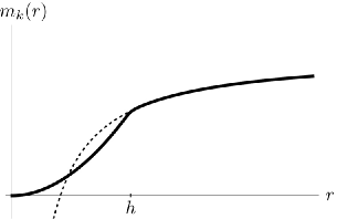
Figure 8: Unlike in the Reissnner Nordstrom case (dashed line), the Komar mass $m_{K}(r)$ is non-singular at the origin, and furthermore obeys the positive energy condition.

A note is now in order. The so-called material energy is a tenable alternative to the Komar mass. Following Weinberg Weinberg , it is the integration of the energy as measured in a locally inertial frame. Technically speaking, one supplements the naive (non-covariant) mass formula by the missing $\sqrt{-g_{tt}g_{rr}}$ factor, to give

$$M_{W}(r)=\frac{1}{G}\int_{0}^{r}e^{\frac{1}{2}(\nu+\lambda)}\left(1+e^{-\lambda}(\lambda^{\prime}r-1)\right)dr~{},$$ (87)

for a spherically symmetric metric. With regard to the present case, it seems that the two mass definitions, Komar mass and Weinberg’s material energy, are distinguished from each other only by their different ${\cal O}(\epsilon)$ corrections.

IX Holographic entropy packing

The geometric anchor connecting us to black hole thermodynamics is the imaginary time periodicity of the Euclidean manifold (or alternatively, the Kruskal $\omega$ parameter which characterizes the Lorentzian manifold), which underlies the Hawking temperature

$$T=\frac{\kappa}{2\pi}=\frac{1}{4\pi h}\left(1-\frac{GQ^{2}}{h^{2}}\right)~{}.$$ (88)

$T=T_{\infty}$ is the temperature at infinity associated with the thermal state of the field theory which lives on the black hole background The striking feature is that, unlike in conventional black hole physics, the exact Hawking periodicity has been recovered in the present theory by defusing the conic defect at the origin, rather that at the event horizon. A variety of related features which include

• ’Near horizon’ like light cone structure eq.(65),

• Equi surface gravity eq.(68),

• Rindler structure eq.(71),

• Kruskal structure eq.(79),

• Universal Komar mass eq.(86),

all point out towards non-trivial physics associated with the black hole interior.

Starting from the Smarr formula Smarr

$$m_{K}(h)=\frac{\kappa}{4\pi}A(h)~{},$$ (89)

or more precisely, from its thermodynamic oriented formulation

$$M-\frac{Q^{2}}{h}=2TS~{},$$ (90)

one first confronts the $\{M,Q\}$ black hole with its $\{M+\Delta M,Q+\Delta Q\}$ extension, to find

$$\Delta M-\frac{Q}{h}\Delta Q=T\Delta S~{}.$$ (91)

The result, as is well known, is the 1st law of charged black hole thermodynamics. Next we multiply eq.(90) by the $r^{2}/h^{2}$ ratio, to obtain a meaningful formula for an inner sphere of circumferential radius $r\leq h$

$$m_{K}^{in}(r)=\frac{\kappa}{4\pi}A(r)~{},$$ (92)

or equivalently

$$\left(M-\frac{Q^{2}}{h}\right)\frac{r^{2}}{h^{2}}=2Tֿ\left(S\frac{r^{2}}{h^{2}}\right)~{},$$ (93)

and attempt to understand its significance. Note that an analogous formula simply does not exist for the interior of ordinary black holes. In some respects, as could already been inferred from the light cone structure, and from the other features on the list at the beginning of this section, the inner spherical surface resembles in some respects a maximally stretched horizon. Consequently, it becomes meaningful to ask what portion $S(r)$ of the total entropy $S\equiv S(h)$ is stored within an arbitrary inner sphere of a finite surface area $A(r)=4\pi r^{2}$ (and most importantly, of a vanishing invariant volume $V(r)\rightarrow 0$) which hosts a Komar mass $M_{K}(r)$? Already at this stage, one can already deduce that

$$\boxed{S(r)=S\frac{r^{2}}{h^{2}}=\frac{\pi r^{2}}{G}}~{},$$ (94)

and appreciate the emerging purely geometrical ’t Hooft-Susskind universal entropy bound eq.(1), and the fact that the bound is locally saturated.

It remains, however, to figure out how exactly does the core configuration change when supplementing the pair $\{M,Q\}$ by tiny amounts $\{\Delta M,\Delta Q\}$, respectively? The crucial point to notice then is that, at the $\epsilon\rightarrow 0$ limit, the resulting configuration appears to be nothing but a linearly stretched version of the former configuration. Exactly in the same way that an ordinary black hole changes it size once $M,Q$ get shifted, meaning $h\rightarrow h+\Delta h$ accordingly, any infinitely thin concentric layer of radius $r$ is puffed up to a new radius $r\rightarrow r+\Delta r$ (see illustration in Fig.9), in such a way that

$$\Delta\left(\frac{r}{h}\right)=0~{}~{}\Longrightarrow~{}~{}\Delta r=\frac{r}{h}\Delta h~{}.$$ (95)

This is a reflection of the fact that, as $\epsilon\rightarrow 0$, the one and only length scale floating around is $h$. Altogether, in analogy with eq.(91), and subject to the geometric rule eq.(95), we have

$$\Delta\left(M\frac{r^{2}}{h^{2}}\right)-\frac{1}{h}\left(Q\frac{r}{h}\right)\Delta\left(Q\frac{r}{h}\right)=T\Delta S(r)~{}.$$ (96)

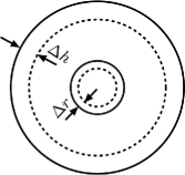
Figure 9: The $\{M+\Delta M,Q+\Delta Q\}$ configuration (solid circles) is a linearly stretched version of the $\{M,Q\}$ configuration (dashed circles). As $h\rightarrow h+\Delta h$, each point at a circumferential radius $r$ gets radially shifted by an amount $\Delta r=\displaystyle{\frac{r}{h}\Delta h}$.

The emerging entropy packing profile turns out to be (i) Locally holographic, i.e. exhibits proportionality to $A(r)$ for every $r\leq h$, and (ii) $M,Q$-independent, and hence universal. The overall picture is then of an onion-like entropy packing model DG . The entropy of any inner sphere is maximally packed, and unaffected by the outer layers. In particular, any additional piece of entropy is maximally packed on its own external layer, with $M,Q$ as well as $M_{K}(r)$ being adjusted accordingly.

An interesting point has to do with the entropy to energy ratio, which is $r$-independent in our case, but is never smaller than $2\pi r$

$$\frac{S(r)}{M_{K}(r)}=\frac{S(h)}{M_{K}(h)}=\frac{\pi h^{2}}{G\left(M-\frac{Q^{2}}{h}\right)}\geq 2\pi r~{}.$$ (97)

This is in apparent violation of Bekenstein’s universal entropy bound Bbound . The reason seems to be the following. Whereas the entropy $S(r)$ of some inner sphere is universal, the associated Komar mass $M_{K}(r)\sim M^{-1}$ is affected by the total mass $M$ of the whole system. Admittedly, Bekenstein’s universal bound is relevant Bviolation only for weakly self gravitating isolated physical systems, and for these it is a much stronger bound than the holographic one.

The various scalings involved may suggest that the holographic entropy packing is indeed a matter of interpretation. To be more explicit, let us examine the issue from the point of view of a physicist who is convinced that general relativity is the fundamental theory of gravity, and therefore is totally unaware of its hereby advocated spontaneously induced nature. Such a physicist (not to be confused with an Einstein frame observer whose metric is $\phi^{-1}g_{\mu\nu}$ rather the $g_{\mu\nu}$) would recast the underlying field equations into their basic Einstein form ${\cal R}_{\mu\nu}-\frac{1}{2}g_{\mu\nu}{\cal R}=8\pi G{\cal T}_{\mu\nu}^{eff}$, moving all terms and factors, save for the Einstein tensor itself, to the r.h.s., thereby defining an effective energy/momentum tensor ${\cal T}_{\mu\nu}^{eff}$. In particular, inside the core, the dynamical Newton constant is given by

$$G_{in}(r)=\frac{1}{\phi(r)}=G\frac{r^{2}}{h^{2}}~{},$$ (98)

but our ’general relativistic’ observer still insists on it being $G$, which requires from his side the effective replacement

$$G\mapsto G\frac{h^{2}}{r^{2}}~{}.$$ (99)

The Hawking temperature, on the other hand, is defined at asymptotic distances, and thus, is fully respected by our ’naive’ observer, that is

$$T\mapsto T~{}.$$ (100)

But this cannot be the case, unless of course

$$GM\mapsto GM~{},~{}GQ^{2}\mapsto GQ^{2}~{}~{}\Longrightarrow~{}~{}h\mapsto h~{}.$$ (101)

In turn, fully consistent with our analysis, the following counter replacements are in order

$$M\mapsto M\frac{r^{2}}{h^{2}}~{},~{}Q\mapsto Q\frac{r}{h}~{}.$$ (102)

All the above nicely converge now back into

$$S=\frac{\pi h^{2}}{G}\mapsto\frac{\pi r^{2}}{G}~{},$$ (103)

which completes the interpretation of an observer ignorant of the local variations of the Newton constant inside the core.

X Summary and outlook

It has come as a big surprise that spontaneously induced general relativity does not always admit a full general relativistic limit. Such an intriguing possibility is demonstrated in this paper at the charged black hole level, where the exterior general relativistic Reissner-Nordstrom solution connects with a novel holographic interior; the phase transition takes then place precisely at the would have been outer event horizon. The new physics associated with the inner core has been discussed in some details, with our main result being the local realization of the ’t Hooft-Susskind-Bousso holographic principle (the holographic bound, as we recall, is not applicable inside ordinary black holes). Notably, this is achieved without invoking string theory and/or the AdS/CFT correspondence. Our results are not sensitive to the exact shape of the scalar potential, thus leaving the door open a more general class of $f(R)$ gravity models, and will only suffer minor modifications upon introducing an optional Brans-Dicke kinetic term.

The emerging maximal entropy packing mechanism sheds new light on how information is stored within a black hole. The interior core, resembling now a maximally stretched horizon, is not a ’boring’ place any more (at least in the sense discussed in the introduction), but has started functioning as Nature’s ultimate information storage. Rather than envision bits of information evenly spread solely on the horizon surface or in its vicinity, a bit per Planck area, they are now universally and holographically spread in the whole black hole interior. Rather than tiling the horizon by Planck area patches, the traditional way it is being done in quantum black hole models, the present work suggests the alternative of filling up the interior with (say) light sheet unit intervals. The overall picture is then of an onion-like entropy packing shell model. Reflecting our main formula eq.(94), the entropy of any inner sphere, being geometric in nature, is maximally packed and unaffected by the outer layers. Any additional entropy is maximally packed on its own external layer, with the overall mass and charge, as well as the intimately related Komar mass distribution eq.(86), being adjusted accordingly. Needless to say, exactly the same structure is expected to hold once the cosmological constant and/or angular momentum enter the game.

A final speculation concerning the value of $\epsilon$, the dimensionless number which parametrizes the deviation from general relativity, is irresistible. Classically, with general relativity so well established, $\epsilon\rightarrow+0$ is indeed the limit to study. However, having quantum mechanics in mind, and appreciating the fact that the singularity at the origin will eventually be disarmed quantum mechanically, it is quite appealing to imagine a very small yet a finite $\epsilon$. For example, the invariant width of the transition region may be fixed by the Planck length, namely

$$\sqrt{\epsilon}h\simeq\ell_{Pl}~{}.$$ (104)

- (1) S.W. Hawking, Phys. Rev. Lett. 26, 1344 (1971); J.D. Bekenstein, Lett. Nuov. Cimento 4, 737 (1972); J.D. Bekenstein, Phys. Rev. D7, 2333 (1973); S.W. Hawking, Nature 248, 30 (1974); J.D. Bekenstein, Phys. Rev. D9, 3292 (1974); S.W. Hawking, Comm. Math. Phys. 43, 199 (1975).
- (2) G.W. Gibbons and S.W. Hawking, Phys. Rev. D15, 2752 (1977).
- (3) R.M. Wald, Phys. Rev. D48, R3427 (1993); V. Iyer and R.M. Wald, Phys. Rev. D50, 846 (1994).
- (4) J. D. Bekenstein, Lett. Nuovo Cim. 11, 467 (1974); V. Mukhanov, Pis. Eksp. Teor. Fiz. 44, 50 (1986) [JETP Lett. 44, 63 (1986)]; J.D. Bekenstein and V.F. Mukhanov, Phys. Lett. B360, 7 (1995).
- (5) K.S. Thorne, W.H. Zurek and R.H. Price, in Black Holes: The Membrane Paradigm, p. 280 (Yale University Press, New Haven, 1986); L. Susskind, L. Thorlacius and J. Uglum, Phys. Rev. D48, 3743 (1993).
- (6) G. ’t Hooft, in Salam festschrifft A. Aly, J. Ellis, and S. Randjbar Daemi eds, (World Scientific, 1993), [arXiv gr-qc/9310026]; L. Susskind, J. Math. Phys. 36, 6377 (1995);
- (7) L. Susskind, Jour. Math. Phys. 36, 6377 (1995); D. Bigatti and L. Susskind, ”Strings, branes and gravity” (Boulder), 883 (1999);
- (8) R. Bousso, Rev. Mod. Phys. 74, 825 (2002).
- (9) J.M. Maldacena, Adv. Theor. Math. Phys. 2, 231 (1998); ibid. Int. Jour. Theor. Phys. 38, 1113 (1999).
- (10) A. Davidson and I. Gurwich, Int. Jour. Mod. Phys. D19, 2345 (2010).
- (11) G. Chapline, E. Hohlfeld, R.B. Laughlin and D.I. Santiago, Int. Jour. Mod. Phys. A18,3587 (2003).
- (12) P.O. Mazur and E. Mottola, Proc. Nat. Acad. Sci. (PNAS) 101, 9545 (2004); C. Barcelo, S. Liberati, S. Sonego and M. Visser, Phys. Rev. D77, 044032 (2008);
- (13) I. Kanitscheider, K. Skenderis and M. Taylor, JHEP 0706:056 (2007); K. Skenderis and M. Taylor, Phys. Rep. 467, 117 (2008).
- (14) A. Davidson and I. Gurwich, Phys. Rev. Lett. 106, 151301 (2011).
- (15) A. Komar, Phys. Rev. 113, 934 (1959).
- (16) S. Weinberg, in Gravitation and Cosmology, (Wiley, 1972), pp. 302-303.
- (17) C.H. Brans and R.H. Dicke, Phys. Rev. 124, 925 (1961).
- (18) A.A. Starobinsky, Phys. Lett. B, 91 (1980); H. Kleinert and H.J. Schmidt, Gen. Rel. Grav. 34, 1295 (2002); S. Capozielo, Int. J. Mod. Phys. D11, 483 (2002); E.E. Flanagan, Class Quant. Grav. 21, 3817 (2004); S.M. Carroll, V. Duvvuri, M. Trodden and M.S. Turner, Phys. Rev. D70, 043528 (2004); G.J. Olmo, Phys. Rev. Lett. 95, 261102 (2005); S. Nojiri and S.D. Odintsov, Int. J. Geom. Meth. Mod. Phys. 4, 115 (2007); E. Barausse, T.P. Sotiriou and J.C. Miller, Class. Quant. Grav. 25, 062001 (2008); For recent reviews see: A. De Felice and S. Tsujikawa, Living Rev. Relativity 13, 3 (2010);
- (19) T.P. Sotiriou and V. Faraoni, Rev. Mod. Phys. 82, 451 (2010).
- (20) T. Padmanabhan, Class. Quant. Grav. 21, 4485 (2004).
- (21) L. Smarr, Phys. Rev. Lett. 30, 71–73 (1973).
- (22) J.D. Bekenstein, Phys. Rev. D23, 287 (1981).
- (23) J.D. Bekenstein, Found. Phys. 35, 1805 (2005).