The WiggleZ Dark Energy Survey: mapping the distance-redshift relation with baryon acoustic oscillations
Abstract
We present measurements of the baryon acoustic peak at redshifts , and in the galaxy correlation function of the final dataset of the WiggleZ Dark Energy Survey. We combine our correlation function with lower-redshift measurements from the 6-degree Field Galaxy Survey and Sloan Digital Sky Survey, producing a stacked survey correlation function in which the statistical significance of the detection of the baryon acoustic peak is - relative to a zero-baryon model with no peak. We fit cosmological models to this combined baryon acoustic oscillation (BAO) dataset comprising six distance-redshift data points, and compare the results to similar fits to the latest compilation of supernovae (SNe) and Cosmic Microwave Background (CMB) data. The BAO and SNe datasets produce consistent measurements of the equation-of-state of dark energy, when separately combined with the CMB, providing a powerful check for systematic errors in either of these distance probes. Combining all datasets we determine for a flat Universe, consistent with a cosmological constant model. Assuming dark energy is a cosmological constant and varying the spatial curvature, we find .
keywords:
surveys, large-scale structure of Universe, cosmological parameters, distance scale, dark energy1 Introduction
**footnotetext: E-mail: cblake@astro.swin.edu.auMeasurements of the cosmic distance-redshift relation have always constituted one of the most important probes of the cosmological model. Eighty years ago such observations provided evidence that the Universe is expanding; more recently they have convincingly suggested that this expansion rate is accelerating. The distance-redshift relation depends on the expansion history of the Universe, which is in turn governed by its physical contents including the properties of the “dark energy” which has been hypothesized to be driving the accelerating expansion. One of the most important challenges in contemporary cosmology is to distinguish between the different possible physical models for dark energy, which include a material or scalar field smoothly filling the Universe with a negative equation-of-state, a modification to the laws of gravity at large cosmic scales, or the effects of inhomogeneity on cosmological observations. Cosmological distance measurements provide one of the crucial observational datasets to help distinguish between these different models.
One of the most powerful tools for mapping the distance-redshift relation is Type Ia supernovae (SNe Ia). About a decade ago, observations of nearby and distant SNe Ia provided some of the most compelling evidence that the expansion rate of the Universe is accelerating (Riess et al. 1998, Perlmutter et al. 1999), in agreement with earlier suggestions based on comparisons of the Cosmic Microwave Background (CMB) and large-scale structure data (Efstathiou, Sutherland & Maddox 1990, Krauss & Turner 1995, Ostriker & Steinhardt 1995). Since then the sample of SNe Ia available for cosmological analysis has grown impressively due to a series of large observational projects which has populated the Hubble diagram across a range of redshifts. These projects include the Nearby Supernova Factory (Copin et al. 2006), the Center for Astrophysics SN group (Hicken et al. 2009), the Carnegie Supernova Project (Hamuy et al. 2006) and the Palomar Transient Factory (Law et al. 2009) at low redshifts ; the Sloan Digital Sky Survey (SDSS) supernova survey (Kessler et al. 2009) at low-to-intermediate redshifts ; the Supernova Legacy Survey (Astier et al. 2006) and ESSENCE (Wood-Vasey et al. 2007) projects at intermediate redshifts ; and observations by the Hubble Space Telescope at high redshifts (Riess et al. 2004, 2007; Dawson et al. 2009). These supernovae data have been collected and analyzed in a homogeneous fashion in the “Union” SNe compilations, initially by Kowalski et al. (2008) and most recently by Amanullah et al. (2010) in the “Union 2” sample of 557 SNe Ia.
The utility of these supernovae datasets is now limited by known (and potentially unknown) systematic errors which could bias cosmological fits if not handled correctly. These systematics include redshift-dependent astrophysical effects, such as potential drifts with redshift in the relations between colour, luminosity and light curve shape owing to evolving SNe Ia populations, and systematics in analysis such as the fitting of light curves, photometric zero-points, K-corrections and Malmquist bias. Although these systematics have been treated very thoroughly in recent supernovae analyses, it is clearly desirable to cross-check the cosmological conclusions with other probes of the distance-redshift relation.
A very promising and complementary method for mapping the distance-redshift relation is the measurement of baryon acoustic oscillations (BAOs) in the large-scale clustering pattern of galaxies, and their application as a cosmological standard ruler (Eisenstein, Hu & Tegmark 1998, Cooray et al. 2001, Eisenstein 2003, Blake & Glazebrook 2003, Seo & Eisenstein 2003, Linder 2003, Hu & Haiman 2003). BAOs correspond to a preferred length scale imprinted in the distribution of photons and baryons by the propagation of sound waves in the relativistic plasma of the early Universe (Peebles & Yu 1970, Sunyaev & Zeldovitch 1970, Bond & Efstathiou 1984, Holtzman 1989, Hu & Sugiyama 1996, Eisenstein & Hu 1998). This length scale, which corresponds to the sound horizon at the baryon drag epoch denoted by , may be predicted very accurately by measurements of the CMB which yield the physical matter and baryon densities that control the sound speed, expansion rate and recombination time in the early Universe: the latest determination is Mpc (Komatsu et al. 2009). In the pattern of late-time galaxy clustering, BAOs manifest themselves as a small preference for pairs of galaxies to be separated by , causing a distinctive “baryon acoustic peak” to be imprinted in the 2-point galaxy correlation function. The corresponding signature in Fourier space is a series of decaying oscillations or “wiggles” in the galaxy power spectrum.
Measurement of BAOs has become an important motivation for galaxy redshift surveys in recent years. The small amplitude of the baryon acoustic peak, and the large size of the relevant scales, implies that cosmic volumes of order 1 Gpc3 must be mapped with of order galaxies to ensure a robust detection (Tegmark 1997, Blake & Glazebrook 2003, Glazebrook & Blake 2005, Blake et al. 2006). Significant detections of BAOs have now been reported by three independent galaxy surveys, spanning a range of redshifts : the SDSS, the WiggleZ Dark Energy Survey, and the 6-degree Field Galaxy Survey (6dFGS).
The most accurate BAO measurements have been obtained by analyzing the SDSS, particularly the Luminous Red Galaxy (LRG) component. Eisenstein et al. (2005) reported a convincing detection of the acoustic peak in the 2-point correlation function of the SDSS Third Data Release (DR3) LRG sample with effective redshift . Percival et al. (2010) performed a power-spectrum analysis of the SDSS DR7 dataset, considering both the main and LRG samples, and measured the distance-redshift relation at both and with accuracy in units of the standard ruler scale. Other studies of the SDSS LRG sample, producing broadly similar conclusions, have been undertaken by Hutsi (2006), Percival et al. (2007), Sánchez et al. (2009) and Kazin et al. (2010a). These studies of SDSS galaxy samples built on hints of BAOs reported by the 2-degree Field Galaxy Redshift Survey (Percival et al. 2001, Cole et al. 2005) and combinations of smaller datasets (Miller et al. 2001). There have also been potential BAO detections in photometric-redshift catalogues from the SDSS (Blake et al. 2007, Padmanabhan et al. 2007, Crocce et al. 2011), although the statistical significance of these measurements currently remains much lower than that which can be obtained using spectroscopic redshift catalogues.
These BAO detections have recently been supplemented by new measurements from two different surveys, which have extended the redshift coverage of the standard-ruler technique. In the low-redshift Universe the 6dFGS has reported a BAO detection at (Beutler et al. 2011). This study produced a measurement of the standard ruler scale and a new determination of the Hubble constant . At higher redshifts the WiggleZ Survey has quantified BAOs at , producing a measurement of the baryon acoustic scale (Blake et al. 2011). Taken together, these different galaxy surveys have demonstrated that BAO standard-ruler measurements are self-consistent with the standard cosmological model established from CMB observations, and have yielded new, tighter constraints on cosmological parameters.
The accuracy with which BAOs may be used to determine the distance-redshift relation using current surveys is limited by statistical rather than systematic errors (in contrast to observations of SNe Ia). The measurement error in the large-scale correlation function, which governs how accurately the preferred scale may be extracted, is determined by the volume of the large-scale structure mapped and the number density and bias of the galaxy tracers. There are indeed potential systematic errors associated with fitting models to the BAO signature, which are caused by the modulation of the pattern of linear clustering laid down in the high-redshift Universe by the non-linear scale-dependent growth of structure, the distortions apparent when the signal is observed in redshift-space and the bias with which galaxies trace the network of matter fluctuations. However, the fact that the BAOs are imprinted on large, linear and quasi-linear scales of the clustering pattern means that these non-linear, systematic distortions are amenable to analytical or numerical modelling and the leading-order effects are well-understood (Eisenstein, Seo & White 2007, Crocce & Scoccimarro 2008, Matsubara 2008, Sánchez, Baugh & Angulo 2008, Smith, Scoccimarro & Sheth 2008, Seo et al. 2008, Padmanabhan & White 2009). As such, BAOs in current datasets are believed to provide a robust probe of the cosmological model, relatively free of systematic error and dominated by statistical errors. In this sense they provide a powerful cross-check of the distance-redshift relation mapped by supernovae.
In this study we report our final analysis of the baryon acoustic peak from the angle-averaged correlation function of the completed WiggleZ Survey dataset, in which we present distance-scale measurements as a function of redshift between and , including a covariance matrix which may be applied in cosmological parameter fits. We also present a new measurement of the correlation function of the SDSS-LRG sample. We stack the 6dFGS, SDSS-LRG and WiggleZ correlation functions to produce the highest-significance detection to date of the baryon acoustic peak in the galaxy clustering pattern. We perform cosmological parameter fits to this latest BAO distance dataset, now comprising data points at six different redshifts. By comparing these fits with those performed on the latest compilation of SNe Ia, we search for systematic disagreements between these two important probes of the distance-redshift relation.
The structure of our paper is as follows: in Section 2 we summarize the three galaxy spectroscopic redshift survey datasets which have provided the most significant BAO measurements. In Section 3 we outline the modelling of the baryon acoustic peak applied in this study. In Section 4 we report the measurement and analysis of the final WiggleZ Survey correlation functions in redshift slices, and in Section 5 we present the new determination of the correlation function of SDSS LRGs. In Section 6 we construct a stacked galaxy correlation function from these surveys and analyze the statistical significance of the BAO detection contained therein. In Section 7 we perform cosmological parameter fits to various combinations of BAO, SNe Ia and CMB data, and we list our conclusions in Section 8.
2 Datasets
2.1 The WiggleZ Dark Energy Survey
The WiggleZ Dark Energy Survey (Drinkwater et al. 2010) is a large-scale galaxy redshift survey of bright emission-line galaxies which was carried out at the Anglo-Australian Telescope between August 2006 and January 2011 using the AAOmega spectrograph (Saunders et al. 2004, Sharp et al. 2006). Targets were selected via joint ultraviolet and optical magnitude and colour cuts using input imaging from the Galaxy Evolution Explorer (GALEX) satellite (Martin et al. 2005), the Sloan Digital Sky Survey (SDSS; York et al. 2000) and the 2nd Red Cluster Sequence (RCS2) Survey (Gilbank et al. 2011). The survey is now complete, comprising of order redshifts and covering of order deg2 of equatorial sky. In this study we analyzed a galaxy sample drawn from our final set of observations, after cuts to maximize the contiguity of each survey region. The sample includes a total of galaxies in the redshift range .
2.2 The 6-degree Field Galaxy Survey
The 6-degree Field Galaxy Survey (6dFGS, Jones et al. 2009) is a combined redshift and peculiar velocity survey covering nearly the entire southern sky with the exception of a band along the Galactic plane. Observed galaxies were selected from the 2MASS Extended Source Catalog (Jarrett et al. 2000) and the redshifts were obtained with the 6-degree Field (6dF) multi-fibre instrument at the U.K. Schmidt Telescope between 2001 and 2006. The final 6dFGS sample contains galaxies distributed over deg2 with a mean redshift of . The analysis of the baryon acoustic peak in the 6dFGS (Beutler et al. 2011) utilized all galaxies selected to . We provide a summary of this BAO measurement in Section 6.1.
2.3 The Sloan Digital Sky Survey Luminous Red Galaxy sample
The SDSS included the largest-volume spectroscopic LRG survey to date (Eisenstein et al. 2001). The LRGs were selected from the photometric component of SDSS, which imaged the sky at high Galactic latitude in five passbands and (Fukugita et al. 1996, Gunn et al. 1998) using a m telescope (Gunn et al. 2006). The images were processed (Lupton et al. 2001, Stoughton et al. 2002, Pier et al. 2003, Ivezic et al. 2004) and calibrated (Hogg et al. 2001, Smith et al. 2002, Tucker et al. 2006), allowing selection of galaxies, quasars (Richards et al. 2002) and stars for follow-up spectroscopy (Eisenstein et al. 2001, Strauss et al. 2002) with twin fibre-fed double spectographs. Targets were assigned to plug plates according to a tiling algorithm ensuring nearly complete samples (Blanton et al. 2003).
The LRG sample serves as a good tracer of matter because these galaxies are associated with massive dark matter halos. The high luminosity of LRGs enables a large volume to be efficiently mapped, and their spectral uniformity makes them relatively easy to identify. In this study we analyze similar LRG catalogues to those presented by Kazin et al. (2010a, 2010b)†††These catalogues and the associated survey mask are publicly available at http://cosmo.nyu.edu/eak306/SDSS-LRG.html, to which we refer the reader for full details of selection and systematics. In particular, in this study we focus on the sample DR7-Full, which corresponds to all LRGs in the redshift range and absolute magnitude range . The sky coverage and redshift distributions of the LRG samples are presented in Figures 1 and 2 of Kazin et al. (2010a). DR7-Full includes LRGs with average redshift , covering total volume Gpc3 with average number density Mpc-3.
3 Modelling the baryon acoustic peak
In this Section we summarize the two models we fitted to the new baryon acoustic peak measurements presented in this study. These models describe the quasi-linear effects which cause the acoustic feature and correlation function shape to deviate from the linear-theory prediction. There are two main aspects to model: a damping of the acoustic peak caused by the displacement of matter due to bulk flows, and a distortion in the overall shape of the clustering pattern due to the scale-dependent growth of structure (Eisenstein et al. 2007, Crocce & Scoccimarro 2008, Matsubara 2008, Sánchez et al. 2008, Smith et al. 2008, Seo et al. 2008, Padmanabhan & White 2009). Our models are characterized by four variable parameters: the physical matter density (where is the matter density relative to the critical density and is the Hubble parameter), a scale distortion parameter , a physical damping scale , and a normalization factor . The models for the correlation function in terms of separation can be written in the form
| (1) |
The physical matter density determines (to first order) both the overall shape of the matter correlation function and the length scale of the standard ruler, by determining the physics before recombination. The scale distortion parameter relates the distance-redshift relation at the effective redshift of the sample to the fiducial value used to construct the correlation function measurement, in terms of the parameter (Eisenstein et al. 2005, Padmanabhan & White 2008, Kazin, Sánchez & Blanton 2011):
| (2) |
where is a composite of the physical angular-diameter distance and Hubble parameter , which respectively govern tangential and radial separations in a cosmological model:
| (3) |
The damping scale quantifies the typical displacement of galaxies from their initial locations in the density field due to bulk flows, resulting in a “washing-out” of the baryon oscillations at low redshift. The normalization factor , marginalized in our analysis, models the effects of linear galaxy bias and large-scale redshift-space distortions.
3.1 Default correlation function model
In our first, default, model we constructed the fiducial correlation function in Equation 1 in a similar manner to Eisenstein et al. (2005) and Blake et al. (2011). First, we generated a linear power spectrum as a function of wavenumber for a given using the CAMB software package (Lewis, Challinor & Lasenby 2000). We fixed the values of the other cosmological parameters using a fiducial model consistent with the latest fits to the Cosmic Microwave Background (Komatsu et al. 2011): Hubble parameter , physical baryon density , primordial spectral index and normalization . We also used the fitting formulae of Eisenstein & Hu (1998) to generate a corresponding “no-wiggles” reference spectrum , possessing a similar shape to but with the baryon oscillation component deleted, which we also use in the clustering model as explained below.
We then incorporated the damping of the baryon acoustic peak caused by the displacement of matter due to bulk flows (Eisenstein et al. 2007, Crocce & Scoccimarro 2008, Matsubara 2008) by interpolating between the linear and reference power spectra using a Gaussian damping term :
| (4) |
The magnitude of the damping coefficient can be estimated for a given value of using the first-order prediction of perturbation theory (Crocce & Scoccimarro 2008):
| (5) |
However, this relation provides only an approximation to the true non-linear damping (Taruya et al. 2010), and we chose to marginalize over as a free parameter in our analysis. We note that is closely related to the parameter defined by Sánchez et al. (2008), in the sense that .
We included the boost in small-scale clustering power due to the non-linear scale-dependent growth of structure using the “halofit” prescription of Smith et al. (2003), as applied to the no-wiggles reference spectrum:
| (6) |
Finally, we transformed into the correlation function appearing in Equation 1:
| (7) |
3.2 Comparison correlation function model
The second, comparison model we considered for the fiducial correlation function was motivated by perturbation theory (Crocce & Scoccimarro 2008, Sánchez et al. 2008):
| (8) |
In this relation is the linear model correlation function corresponding to the linear power spectrum . The symbol denotes convolution by the Gaussian damping , which we evaluated as
| (9) | |||||
and is defined by Equation 32 in Crocce & Scoccimarro (2008):
| (10) |
where is the spherical Bessel function of order 1. (fixed in our analysis) is a “mode-coupling” term that restores the small-scale shape of the correlation function and causes a slight shift in the peak position compared to the linear-theory prediction. The model of Equation 8 has been shown to yield unbiased results in baryon acoustic peak fits by Sánchez et al. (2008, 2009).
4 WiggleZ baryon acoustic peak measurements in redshift slices
In this Section we describe our measurement and fitting of the baryon acoustic peak in the WiggleZ Survey galaxy correlation function in three overlapping redshift ranges: , and . Our methodology closely follows that employed by Blake et al. (2011), to which we refer the reader for full details.
4.1 Correlation function measurements
We measured the angle-averaged 2-point correlation function for each WiggleZ survey region using the Landy-Szalay (1993) estimator:
| (11) |
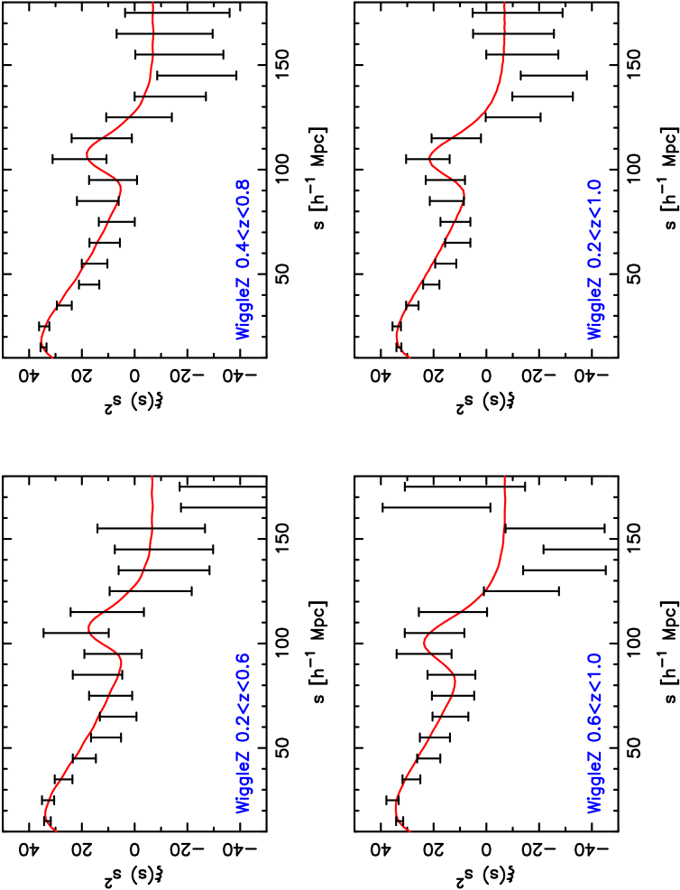
where , and are the data-data, data-random and random-random weighted pair counts in separation bin , where each random catalogue contains the same number of galaxies as the real dataset. We assumed a fiducial flat CDM cosmological model with matter density to convert the galaxy redshifts and angular positions to spatial co-moving co-ordinates. In the construction of the pair counts each data or random galaxy was assigned a weight , where is the survey number density at the location of the th galaxy (determined by averaging over many random catalogues) and Mpc3 is a characteristic power spectrum amplitude at the physical scales of interest. The and pair counts were determined by averaging over 10 random catalogues, which were constructed using the selection-function methodology described by Blake et al. (2010). We measured the correlation function in Mpc separation bins in three overlapping redshift slices , and . The effective redshift of the correlation function measurement in each slice was determined as the weighted mean redshift of the galaxy pairs in the separation bin Mpc, where the redshift of a pair is simply the average , and the weighting is where is defined above. For the three redshift slices in question we obtained values , and .
We determined the covariance matrix of the correlation function measurement in each survey region using an ensemble of 400 lognormal realizations, using the method described by Blake et al. (2011). Lognormal realizations provide a reasonably accurate galaxy clustering model for the linear and quasi-linear scales which are important for the modelling of baryon oscillations. They are more reliable than jack-knife errors, which provide a poor approximation for the correlation function variance on BAO scales because the pair separations of interest are usually comparable to the size of the jack-knife regions, which are then not strictly independent. We note that the lognormal covariance matrix only includes the effects of the survey window function, and neglects the covariance due to the non-linear growth of structure and redshift-space effects. The full non-linear covariance matrix may be studied with the aid of a large set of N-body simulations (Rimes & Hamilton 2005, Takahashi et al. 2011). Work is in progress to construct such a simulation set for WiggleZ galaxies, although this is a challenging computational problem because the typical dark matter haloes hosting the star-forming galaxies mapped by WiggleZ are times lower in mass than the Luminous Red Galaxy sample described in Section 5, requiring high-resolution large-volume simulations. However, we note that Takahashi et al. (2011) demonstrated that the impact of using the full non-linear covariance matrix on the accuracy of extraction of baryon acoustic oscillations is small, so we do not expect our measurements to be compromised significantly through using lognormal realizations to estimate the covariance matrix.
We combined the correlation function measurements and corresponding covariance matrices for the different survey regions using optimal inverse-variance weighting in each separation bin (see equations 8 and 9 in White et al. 2011):
| (12) |
| (13) |
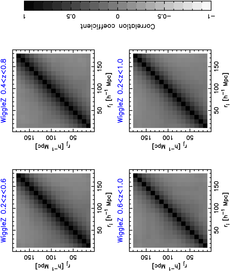
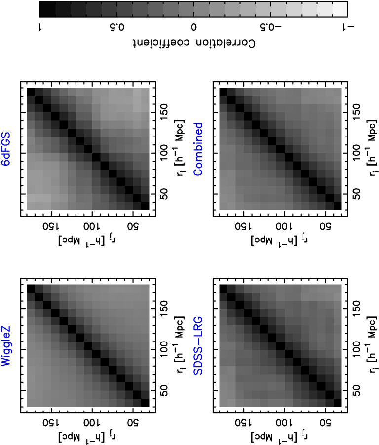
In these equations, and are vectors representing the correlation function measurements in region and the optimally-combined correlation function, and and are the covariance matrices corresponding to these two measurement vectors (with inverses and ). This method produces an almost identical result to combining the individual pair counts and then estimating the correlation function using Equation 11. The combined correlation functions in the three redshift slices are displayed in Figure 1, together with a total WiggleZ correlation function for the whole redshift range which was constructed by combining the separate measurements for and . The corresponding lognormal covariance matrices for each measurement are shown in Figure 2.
4.2 Parameter fits
We fitted the first, default correlation function model described in Section 3 to the WiggleZ measurements in redshift slices , and , varying , , and . Our default fitting range was Mpc (following Eisenstein et al. 2005), where Mpc is an estimate of the minimum scale of validity for the quasi-linear theory described in Section 3. This minimum scale is a quantity which depends on the survey redshift and galaxy bias (which control the amplitude of the non-linear, scale-dependent contributions to the shape of the correlation function) together with the signal-to-noise of the measurement. When fitting Equation 7 to the WiggleZ Survey correlation function we find no evidence for a systematic variation in the derived BAO parameters when we vary the minimum fitted scale over the range Mpc.
We minimized the statistic using the full data covariance matrix derived from lognormal realizations. The fitting results, including the marginalized parameter measurements, are displayed in Table 1. The minimum values of for the model fits in the three redshift slices were , and for 13 degrees of freedom, indicating that our model provides a good fit to the data. The best-fitting scale distortion parameters, which provide the value of for each redshift slice, are all consistent with the fiducial distance-redshift model (a flat CDM Universe with ) with marginalized errors of , and in the three redshift slices. The best-fitting matter densities are consistent with the latest analyses of the CMB (Komatsu et al. 2011). The damping parameters are not well-constrained using our data, but the allowed range is consistent with the predictions of Equation 5 for our fiducial model (which are Mpc for the three redshift slices). When fitting we only permit it to vary over the range .
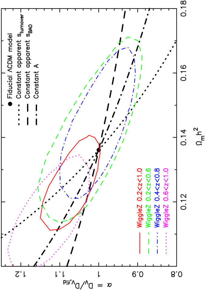
The 2D probability contours for and , marginalizing over and , are displayed in Figure 3. The measurement of (hence ) is significantly correlated with the matter density, which controls the shape of the clustering pattern.
We indicate three degeneracy directions in the parameter space of Figure 3. The first direction (the dashed line) corresponds to a constant measured acoustic peak separation, i.e. , where is the sound horizon at the drag epoch as a function of , determined using the fitting formula quoted in Equation 12 of Percival et al. (2010). This parameter degeneracy would be expected in the case that just the baryon acoustic peak is driving the model fits, such that the measured low-redshift distance is proportional to the standard ruler scale .
The second direction (the dotted line) illustrated in Figure 3 represents the degeneracy resulting from a constant measured shape of a Cold Dark Matter (CDM) power spectrum, i.e. . We note here the consistency between this scaling and the “shape parameter” used to parameterize the CDM transfer function (Bardeen et al. 1986). This shape parameter assumes that wavenumbers are observed in units of Mpc-1, but the standard ruler scale encoded in baryon acoustic oscillations is calibrated by the CMB in units of Mpc, with no factor of .
The third direction (the dash-dotted line) shown in Figure 3, which best describes the degeneracy in our data, corresponds to a constant value of the acoustic parameter introduced by Eisenstein et al. (2005),
| (14) |
which appears in Figure 3 as . We note that the values of predicted by any cosmological model are independent of , because is proportional to .
The acoustic parameter provides the most appropriate description of the distance-redshift relation determined by a BAO measurement in which both the clustering shape and acoustic peak are contributing toward the fit, such that the whole correlation function is being used as a standard ruler (Eisenstein et al. 2005, Sánchez et al. 2008, Shoji et al. 2009). In this case, the resulting measurement of is approximately uncorrelated with . We repeated our BAO fit to the WiggleZ correlation functions in redshift slices using the parameter set . The marginalized values of we obtained are quoted in Table 1, and correspond to measurements of the acoustic parameter with accuracies , and in the three redshift slices.
We also fitted our data with the parameter set , where . Results are again listed in Table 1, corresponding to measurements of with accuracies , and in the three redshift slices. We note that, unlike for the case of , these measurements of are correlated with the matter density , due to the orientation of the parameter degeneracy directions in Figure 3 (noting that constant corresponds to the “constant measured acoustic peak” case defined above).
| Sample | ||||||||
|---|---|---|---|---|---|---|---|---|
| [Mpc] | [ Mpc] | |||||||
| WiggleZ - | ||||||||
| WiggleZ - | ||||||||
| WiggleZ - | ||||||||
| WiggleZ - |
As a check for systematic modelling errors, we repeated the fits to the WiggleZ correlation functions using the second acoustic peak model described in Section 3, motivated by perturbation theory, fitting the data over the same range of scales. The marginalized measurements of in the three redshift slices were , to be compared with the results for the default model quoted in Table 1. The amplitude of the systematic error in the fitted scale distortion parameter is hence significantly lower than the statistical error in the measurement (by at least a factor of 3 in all cases).
We assessed the statistical significance of the BAO detections in each redshift slice by repeating the parameter fits replacing the model correlation function with one generated using the “no-wiggles” reference power spectrum as a function of (Eisenstein & Hu 1998). The minimum values obtained for the statistic for the fits in the three redshift slices were , and , indicating that the model containing baryon oscillations was favoured by , and (with the same number of parameters fitted). These intervals correspond to detections of the baryon acoustic peaks in the redshift slices with statistical significances between - and -. We note that the marginalized uncertainty in the scale distortion parameter for the no-wiggles model fit degrades by a factor of between two and three compared to the fit to the full model, demonstrating that the acoustic peak is very important for establishing the distance constraints from our measurements.
We used the same approach to determine the statistical significance of the BAO detection in the full WiggleZ redshift span , after combining the correlation function measurements in the redshift slices and . In this case the model containing baryon oscillations was favoured by , corresponding to a statistical significance of - for the detection of the baryon acoustic peak.
4.3 Covariances between redshift slices
We used the ensemble of lognormal realizations to quantify the covariance between the BAO measurements in the three overlapping WiggleZ redshift slices. For each of the 400 lognormal realizations in every WiggleZ region, we measured correlation functions for the redshift ranges , and and combined these correlation functions for the different regions using inverse-variance weighting. We then fitted the default clustering model described in Section 3 to each of the 400 combined correlation functions for the three redshift slices.
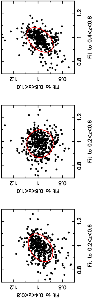
Figure 4 displays the correlations between the 400 marginalized values of the scale-distortion parameter for every pair of redshift slices. As expected, significant correlations are found in the values of obtained from fits to the overlapping redshift ranges and , whereas the fits to the non-overlapping pair produce an uncorrelated measurement (within the statistical noise). The corresponding correlation coefficients for the overlapping pairs are and , where in terms of the covariances . Table 2 contains the resulting inverse covariance matrix for the measurements of in the three redshift slices, that should be used in cosmological parameter fits.
| Redshift slice | |||
|---|---|---|---|
4.4 Comparison to mock galaxy catalogue
As a further test for systematic errors in our distance scale measurements we fitted our BAO models to a dark matter halo catalogue generated as part of the Gigaparsec WiggleZ (GiggleZ) simulation suite (Poole et al., in prep.). The main GiggleZ simulation consists of a particle dark matter N-body calculation in a box of side 1 Gpc. The cosmological parameters used for the simulation initial conditions were .
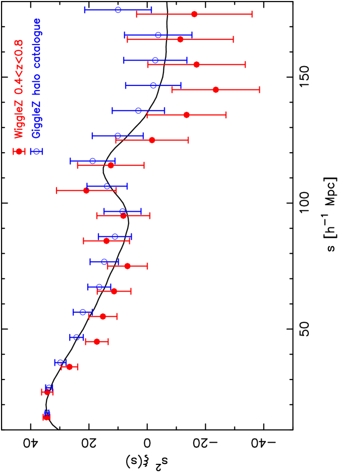
We measured the redshift-space correlation function of a mass-limited subset of the dark matter halo catalogue extracted from the snapshot. This subset of dark matter haloes, spanning a small range of maximum circular velocities around 125 km/s, was selected to possess a similar large-scale clustering amplitude to the WiggleZ galaxies at that redshift. We obtained the covariance matrix of the measurement using jack-knife techniques. We fitted our default correlation function model described in Section 3 to the result, varying , , and and using the same fitting range as the WiggleZ measurement, Mpc.
Figure 5 shows the GiggleZ halo correlation function measurement compared to the WiggleZ correlation function for the redshift range (which was plotted in the top right-hand panel of Figure 1). We overplot the best-fitting default correlation function model for the GiggleZ data. The 2D probability contours for and are displayed in Figure 6, again compared to the WiggleZ measurement and indicating the same degeneracy directions as shown in Figure 3. We conclude that the best-fitting parameter values are consistent with the input values of the simulation (within the statistical error expected in a measurement that uses a single realization) and there is no evidence for significant systematic error. We note that the effective volume of the halo catalogue is slightly greater than that of the WiggleZ survey redshift range , hence the BAO measurements are more accurate in the case of GiggleZ.

5 Baryon acoustic peak measurement from the full Sloan Digital Sky Survey Luminous Red Galaxy sample
In this Section we measure and fit the correlation function of the SDSS-LRG DR7-Full sample. This analysis is similar to that performed by Kazin et al. (2010a) for quasi-volume-limited sub-samples with , but now extended to a higher maximum redshift . We note that we assume a fiducial cosmology for this analysis, motivated by the cosmological parameters used in the LasDamas simulations (which we use to determine the covariance matrix of the measurement as described below in Section 5.2). The choice instead of , as used for the 6dFGS and WiggleZ analyses, would yield very similar results because the Alcock-Paczynski distortion between these cases is negligible compared to the statistical errors in .
5.1 Correlation function measurement
We measured the correlation function of the SDSS-LRG DR7-Full sample by applying the estimator of Equation 11, using random catalogues constructed in the manner described in detail by Kazin et al. (2010a). For the purposes of the model fits in this Section we used separation bins of width Mpc spanning the range Mpc, although we also determined results in Mpc bins in order to combine with the 6dFGS and WiggleZ correlation functions in Section 6 below. The measurement of the DR7-Full correlation function in Mpc bins is displayed in the left-hand panel of Figure 7, where the error bars are determined from the diagonal elements of the covariance matrix of 160 mock realizations, generated as described below in Section 5.2. The solid and dashed lines in Figure 7 are two best-fitting models, determined as explained below in Section 5.3.
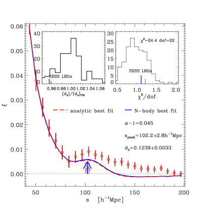
The correlation function measurements in the separation range Mpc are higher than expected in the best-fitting model. However, it is important to remember that these data points are correlated. The reduced chi-squared statistics corresponding to these models are /dof (for 22 degrees of freedom), which fall well within the distribution of found in individual fits to the 160 mock catalogues, as shown in the right-hand inset in Figure 7. Kazin et al. (2010a) discussed the excess clustering measurement in SDSS-LRG subsamples and suggested that this is likely to result from sample variance. This is now reinforced by the fact that the independent-volume measurements from the WiggleZ and 6dFGS samples do not show similar trends of excess (see Figure 8).
A potential cause of the stronger-than-expected clustering of LRGs on large scales is the effect of not masking faint stars on random-catalogue generation. Ross et al. (2011) showed that apparent excess large-scale angular clustering measured in photometric LRG samples (Blake et al. 2007, Padmanabhan et al. 2007, Thomas et al. 2011) is a systematic effect imprinted by anti-correlations between faint stars and the galaxies, that can be corrected for by masking out regions around the stars. However, in the sparser SDSS-DR7 LRG sample the faint stars are uncorrelated with the galaxies at the angles of interest and do not introduce significant systematic errors in the measured correlation function (A.Sánchez, private communication).
5.2 LasDamas mock galaxy catalogues
We simulated the SDSS-LRG correlation function measurement and determined its covariance matrix using the mock galaxy catalogues provided by the Large Suite of Dark Matter Simulations (LasDamas, McBride et al. in prep.). These N-body simulations were generated using cosmological parameters consistent with the WMAP 5-year fits to the CMB fluctuations (Komatsu et al. 2009): .
The LasDamas collaboration generated realistic LRG mock catalogues‡‡‡http://lss.phy.vanderbilt.edu/lasdamas/ by placing galaxies inside dark matter halos using a Halo Occupation Distribution (HOD; Berlind & Weinberg 2002). The HOD parameters were chosen to reproduce the observed galaxy number density as well as the projected two-point correlation function of the SDSS-LRG sample at separations Mpc. We used a suite of 160 LRG mock catalogues constructed from light cone samples with a mean number density Mpc-3. Each DR7-Full mock catalogue covers the redshift range and reproduces the SDSS angular mask, corresponding to a total volume Gpc3. The mock catalogues were subsampled to match the observed redshift distribution of the LRGs.
5.3 Correlation function modelling
We extracted the scale of the baryon acoustic feature in the DR7-Full correlation function measurement by fitting for the scale distortion parameter relative to a template correlation function using Equation 1, fitting over the separation range Mpc. Together with the two correlation function models already described in Section 3, the availability of the suite of LasDamas mock catalogues allows us to add a third template to use as : the mock-mean correlation function of all realizations, which includes effects due to the non-linear growth of structure, redshift-space distortions, galaxy bias, light-coning and the observed 3D mask.
The best-fitting model taking , marginalizing over the correlation function amplitude, is displayed as the solid line in Figure 7, corresponding to . The statistic of the best fit is (for 22 degrees of freedom). The most likely baryon acoustic peak position (determined using the method of Kazin et al. 2010a) is Mpc (represented by the large arrow in Figure 7), where the quoted error is based on the sample variance determined by performing the same analysis on all 160 mock catalogues. The corresponding measurement of the distilled BAO parameter is . The distribution of measurements of for the 160 mocks is shown as the left-hand inset in Figure 7. We do not expect the SDSS result (vertical lines) to coincide with unity, because of the difference between the true and fiducial cosmological parameters.
As a comparison, we also fitted to these data the two correlation function models described in Section 3, parameterized by . The marginalized measurements of for the two models were and , consistent with our determination based on the mock-mean correlation function (which effectively uses fixed values of and ).
Our best-fitting analytic perturbation-theory model due to Crocce & Scoccimarro (2008) is displayed as the red dashed line in the left-hand panel of Figure 7. In this model we find that the best-fitting value of is correlated with , although such changes produce offsets smaller than the 1- statistical error in (represented by the grey region around the short arrows in Figure 7).
5.4 Significance of detection of the SDSS-LRG baryon acoustic feature
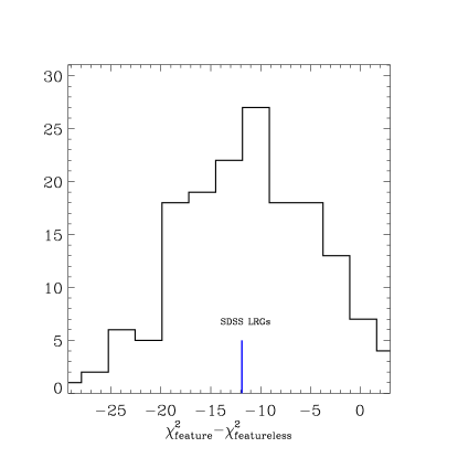
We assessed the statistical significance of the detection of the baryon acoustic peak in the SDSS-LRG sample in a similar style to the WiggleZ analysis described in Section 4.2, by comparing the best-fitting values of for models containing a baryon acoustic feature () and featureless models () constructed using the “no-wiggles” power spectrum of Eisenstein & Hu (1998). We used the perturbation-theory model for the baryon acoustic peak described in Section 3 when constructing these models.
The SDSS-LRG dataset produced over the separation range Mpc, corresponding to a detection of the baryon acoustic feature with significance of -. The histogram resulting from repeating this analysis for all mocks is displayed in the right-hand panel of Figure 7, following Cabre & Gaztanaga (2011); we see that the SDSS result is as expected from an average realization.
We used the same method to compare the significance of detection of the acoustic peak in DR7-Full with that obtained in the volume-limited LRG sub-samples analyzed by Kazin et al. (2010a). The sample “DR7-Sub”, a quasi-volume-limited LRG catalogue spanning redshift range and luminosity range , yields a detection significance of -. For the sample “DR7-Bright”, a sparser volume-limited catalogue with a brighter luminosity cut , the significance of the baryon acoustic feature is just below 2-.
6 The stacked baryon acoustic peak
Our goal in this Section is to assess the overall statistical significance with which the baryon acoustic peak is detected in the combination of current galaxy surveys. In order to do this we combined the galaxy correlation functions measured from the WiggleZ Survey, the Sloan Digital Sky Survey Luminous Red Galaxy (SDSS-LRG) sample and the 6-degree Field Galaxy Survey (6dFGS), and fitted the models described in Section 3 to the result. Although we acknowledge that model fits to a combination of correlation functions obtained using different redshifts and galaxy types will produce parameter values that evade an easy physical interpretation, the resulting statistical significance of the BAO detection remains a quantity of interest.
6.1 The 6dFGS baryon acoustic peak measurement
For completeness we summarize here the measurement of the baryon acoustic peak from the 6dFGS reported by Beutler et al. (2011). After optimal weighting of the data to minimize the correlation function error at the baryon acoustic peak, the 6dFGS sample covered an effective volume Gpc3 with effective redshift . Beutler et al. fitted the model defined by our Equation 8 to the 6dFGS correlation function, using lognormal realizations to determine the data covariance matrix and varying the parameter set , , and . The model fits were performed over the separation range Mpc, with checks made that the best-fitting parameters were not sensitive to the minimum separation employed. The resulting measurements of the distance scale were quantified as Mpc, or . The statistical significance of the detection of the acoustic peak was estimated to be -, based on the difference in chi-squared between the best-fitting model and the corresponding best fit of a zero-baryon model.
6.2 The combined correlation function
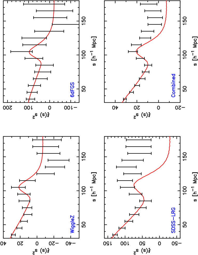
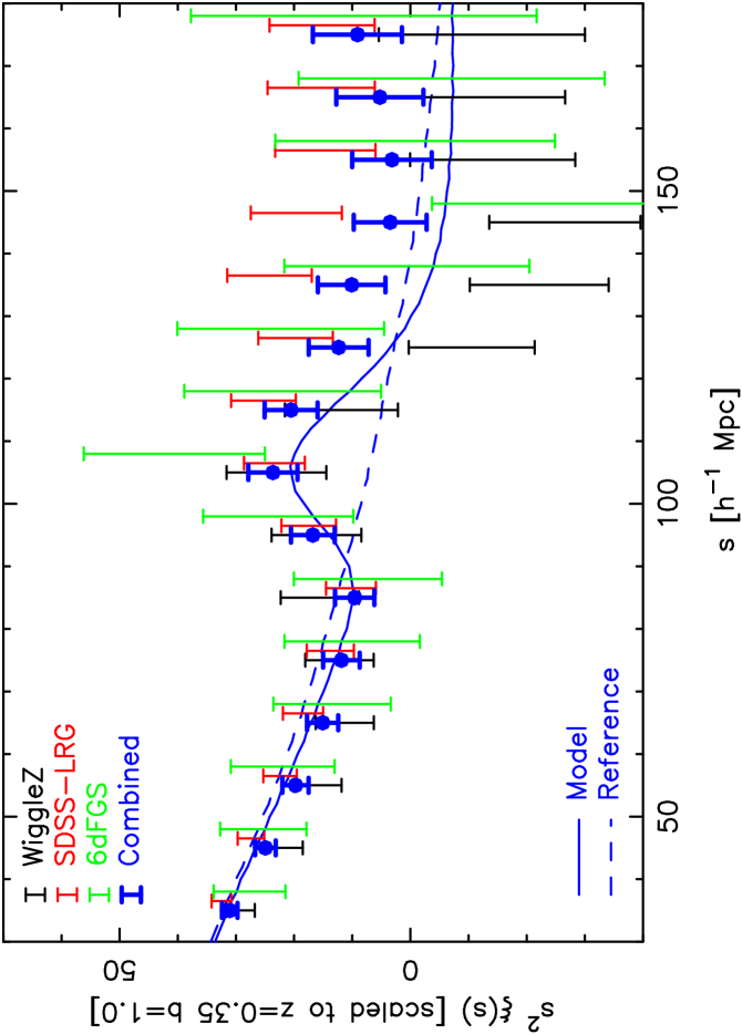
Figure 8 displays the three survey correlation functions combined in our study: the WiggleZ measurement plotted in the lower right-hand panel of Figure 1, the 6dFGS correlation function reported by Beutler et al. (2011), and the SDSS-LRG DR7-Full measurement described in Section 5 (using a binning of Mpc in all cases). These correlation functions have quite different amplitudes owing to differences between the growth factors at the effective redshifts of the samples and the bias factors of the various galaxy tracers. Before stacking these functions we make an amplitude correction to a common redshift and bias factor , by multiplying each correlation function by where is the linear growth factor at redshift and is the Kaiser boost factor in terms of the redshift-space distortion parameter (Kaiser 1987). When calculating these quantities we assumed that the redshifts of the WiggleZ, SDSS-LRG and 6dFGS samples were and the bias factors were . After making these normalization corrections we then combined the correlation functions and their corresponding covariance matrices using inverse-variance weighting in the same style as Equations 12 and 13. The resulting total correlation function is plotted in the lower right-hand panel of Figure 8. The covariance matrices of the different survey correlation functions and final combination are displayed in Figure 9. An additional overplot of these correlation functions is provided in Figure 10. We note that although the SDSS-LRG correlation function measurement used the fiducial cosmology , compared to the choice for the WiggleZ and 6dFGS analyses, the Alcock-Paczynski distortion between these cases is negligible compared to the statistical errors in .
6.3 Significance of the detection of the baryon acoustic peak in the combined sample
We fitted the clustering model described in Section 3 to the combined correlation function over separation range Mpc, varying , , and and using an effective redshift . We used the more conservative minimum fitted scale Mpc for the analysis of the stacked correlation function in this Section, compared to Mpc for the fits to the WiggleZ correlation function in Section 4, because (1) the required non-linear corrections become more important for galaxy samples such as the 6dFGS and SDSS LRGs, which are both more biased and at lower redshift than the WiggleZ sample, and (2) systematic errors in the fitting become relatively more important for this combined dataset with higher signal-to-noise. Although we fixed the relative bias factors of the galaxy samples when stacking the survey correlation functions in Section 6.2, we still marginalized over an absolute normalization when fitting the model in this Section.
We obtained a good fit to the stacked correlation function with (for 11 degrees of freedom) and marginalized parameter values , and Mpc. Although the best-fitting value of must be interpreted as some effective value integrating over redshift, we can conclude that the measured BAO distance scale is consistent with the fiducial model.
We quantified the significance of the detection of the acoustic peak in the combined sample using two methods. Firstly, we repeated the parameter fit replacing the model correlation function with one generated using a “no-wiggles” reference power spectrum (Eisenstein & Hu 1998). The minimum value obtained for the statistic in this case was , indicating that the model containing baryon oscillations was favoured by . This corresponds to a detection of the acoustic peak with a statistical significance of -.
As an alternative approach for assessing the significance of the detection, we changed the fiducial baryon density to and repeated the parameter fit. For zero baryon density we generated the model matter power spectrum using the fitting formulae of Eisenstein & Hu (1998), rather than using the CAMB software. The minimum value obtained for the statistic was now , this time suggesting that the acoustic peak had been detected with a significance of -. The reason that the significance of detection varies between these two methods of assessment is that in the latter case, where the baryon density is changed, the overall shape of the clustering pattern is also providing information used to disfavour the model, whereas in the former case only the presence of the acoustic peak varies between the two sets of models.
7 Cosmological parameter fits
In this Section we fit cosmological models to the latest distance datasets comprising BAO, supernovae and CMB measurements. Our aim is to compare parameter fits to BAO+CMB data (excluding supernovae) and SNe+CMB data (excluding BAO) as a robust check for systematic errors in these distance probes.
7.1 BAO dataset
The latest BAO distance dataset, including the 6dFGS, SDSS and WiggleZ surveys, now comprises BAO measurements at six different redshifts. These data are summarized in Table 3. Firstly, we use the measurement of from the 6dFGS reported by Beutler et al. (2011). Secondly, we add the two correlated measurements of and determined by Percival et al. (2010) from fits to the power spectra of LRGs and main-sample galaxies in the SDSS (spanning a range of wavenumbers Mpc-1). The correlation coefficient for these last two measurements is . We note that our own LRG baryon acoustic peak measurements reported above in Section 5 are entirely consistent with these fits. Finally, we include the three correlated measurements of , and reported in this study, using the inverse covariance matrix listed in Table 2.
In our cosmological model fitting we assume that the BAO distance errors are Gaussian in nature. Modelling potential non-Gaussian tails in the likelihood is beyond the scope of this paper, although we note that they may not be negligible (Percival et al. 2007, Percival et al. 2010, Bassett & Afshordi 2010). We caution that the 2- confidence regions displayed in the Figures in this Section might not necessarily follow the Gaussian scaling. The WiggleZ and SDSS-LRG surveys share a sky overlap of deg2 for redshift range ; given that the SDSS-LRG measurement is derived across a sky area deg2 and the errors in both measurements contain a significant component due to shot noise, the resulting covariance is negligible.
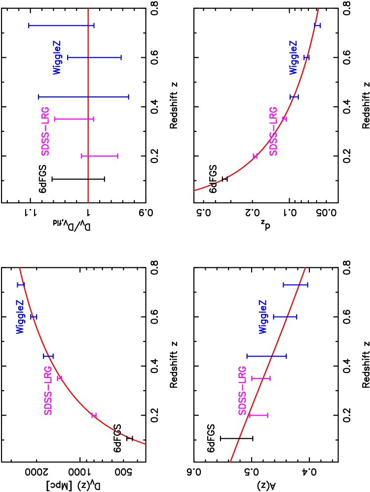
This BAO distance dataset is plotted in Figure 11 relative to a flat CDM cosmological model with matter density and Hubble parameter (these values provide the best fit to the combined cosmological datasets as discussed below). The panels of Figure 11 show various representations of the BAO dataset including and the distilled parameters and .
| Sample | |||
|---|---|---|---|
| 6dFGS | |||
| SDSS | |||
| SDSS | |||
| WiggleZ | |||
| WiggleZ | |||
| WiggleZ |
7.2 SNe dataset
We used the “Union 2” compilation by Amanullah et al. (2010) as our supernova dataset, obtained from the website http://supernova.lbl.gov/Union. This compilation of 557 supernovae includes data from Hamuy et al. (1996), Riess et al. (1999, 2007), Astier et al. (2006), Jha et al. (2006), Wood-Vasey et al. (2007), Holtzman et al. (2008), Hicken et al. (2009) and Kessler et al. (2009). The data is represented as a set of values of the distance modulus for each supernova
| (15) |
where is the luminosity distance at redshift . The values of are reported for a particular choice of the normalization , which is marginalized as an unknown parameter in our analysis as described below. When fitting cosmological models to these SNe data we used the full covariance matrix of these measurements including systematic errors, as reported by Amanullah et al. (2010).
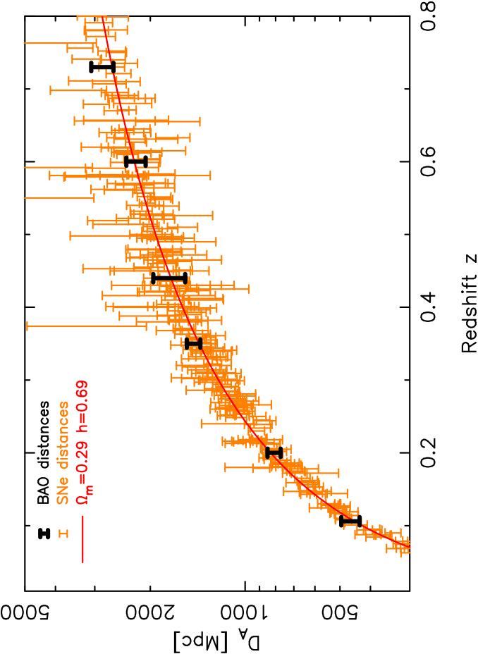
Figure 12 is a representation of the consistency and relative accuracy with which baryon oscillation measurements and supernovae currently map out the cosmic distance scale. In order to construct this figure we converted the BAO measurements of into assuming a Hubble parameter for a flat CDM model with and . The binned supernovae data currently measure the distance-redshift relation at with times higher accuracy than the BAOs, although we note that the consequences for cosmological parameter fits are highly influenced by the differing normalization of the two methods. The supernovae measure the relative luminosity distance to the relation at , , owing to the unknown value of the standard-candle absolute magnitude . The BAOs measure a distance scale relative to the sound horizon at baryon drag calibrated by the CMB data, effectively an absolute measurement of given that the error is dominated by the statistical uncertainty in the clustering fits, rather than any systematic uncertainty in the sound horizon calibration from the CMB.
When undertaking cosmological fits to the supernovae dataset, we performed an analytic marginalization over the unknown absolute normalization (Goliath et al. 2001, Bridle et al. 2002). This is carried out by determining the chi-squared statistic for each cosmological model as
| (16) |
where is the vector representing the difference between the distance moduli of the data and model, and is the inverse covariance matrix for the supernovae distance moduli.
7.3 CMB dataset
We included the CMB data in our cosmological fits using the Wilkinson Microwave Anisotropy Probe (WMAP) “distance priors” (Komatsu et al. 2009) using the 7-year WMAP results reported by Komatsu et al. (2011). The distance priors quantify the complete CMB likelihood via a 3-parameter covariance matrix for the acoustic index , the shift parameter and the redshift of recombination , as given in Table 10 of Komatsu et al. (2011). When deriving these quantities we assumed a physical baryon density , a CMB temperature and a number of relativistic degrees of freedom .
7.4 Flat models
We first fitted a flat CDM cosmological model in which spatial curvature is fixed at but the equation-of-state of dark energy is varied as a free parameter. We fitted for the three parameters using flat, wide priors which extend well beyond the regions of high likelihood and have no effect on the cosmological fits. The best-fitting model has for 563 degrees of freedom, representing a good fit to the distance dataset.
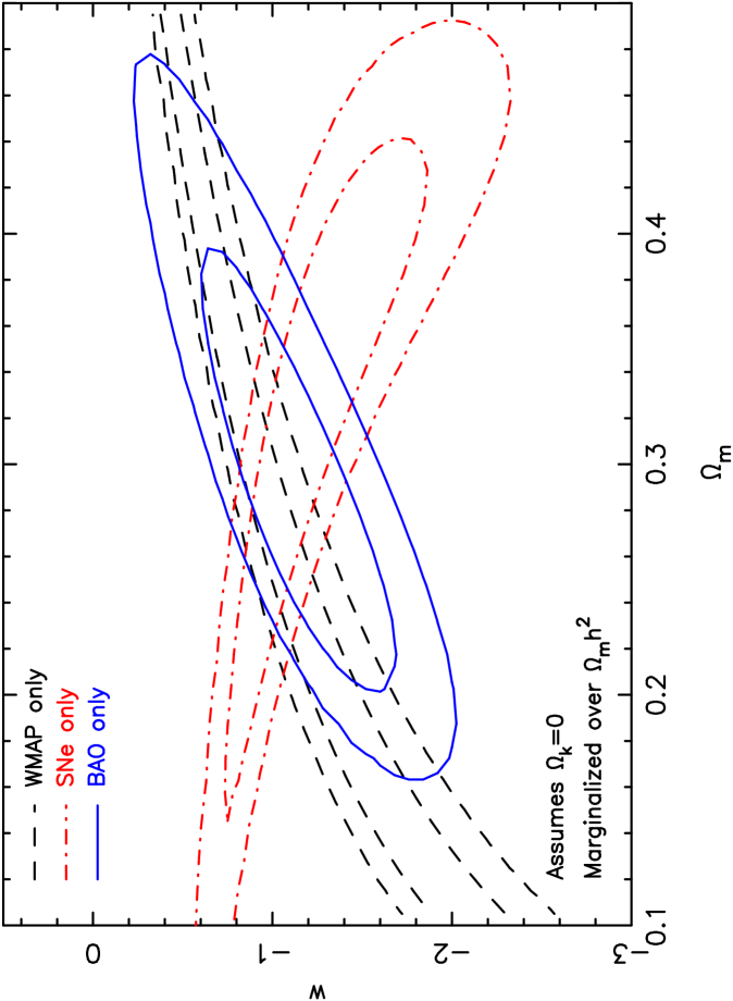
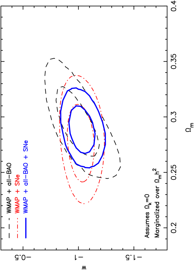
Figures 13 and 14 compare the joint probability of and , marginalizing over , for the individual WMAP, BAO and SNe datasets along with various combinations. We note that for the “BAO only” contours in Figure 13, we have not used any CMB calibration of the standard ruler scale , and thus the 6dFGS and SDSS measurements of do not contribute strongly to these constraints. Hence the addition of the CMB data in Figure 14 has the benefit of both improving the information from the measurements by determining , and contributing the WMAP distance prior constraints. The WMAP+BAO and WMAP+SNe data produce consistent determinations of the cosmological parameters, with the error in the equation-of-state . Combining all three datasets produces the marginalized result (errors in the other parameters are listed in Table 4; the quoted error in results from fitting the three parameters , and ). The best-fitting equation-of-state is consistent with a cosmological constant model for which .
We caution that the probability contours plotted in Figures 13 and 14 (and other similar Figures in this Section) assume that the errors in the BAO distance dataset are Gaussian. If the likelihood contains a significant non-Gaussian tail, the 2- region could be affected.
We repeated the WMAP+BAO fit comparing the two different implementations of the SDSS-LRG BAO distance-scale measurements: the Percival et al. (2010) power spectrum fitting at and , and our correlation function fit presented in Section 5. We found that the marginalized measurements of in the two cases were and , respectively. Our results are therefore not significantly changed by the methodology used for these LRG fits.
7.5 Curved models
We next fitted a curved CDM model, in which we fixed the equation-of-state of dark energy at but added the spatial curvature as an additional free parameter. We fitted for the three parameters using flat, wide priors which extend well beyond the regions of high likelihood and have no effect on the cosmological fits. The best-fitting model has for 563 degrees of freedom.
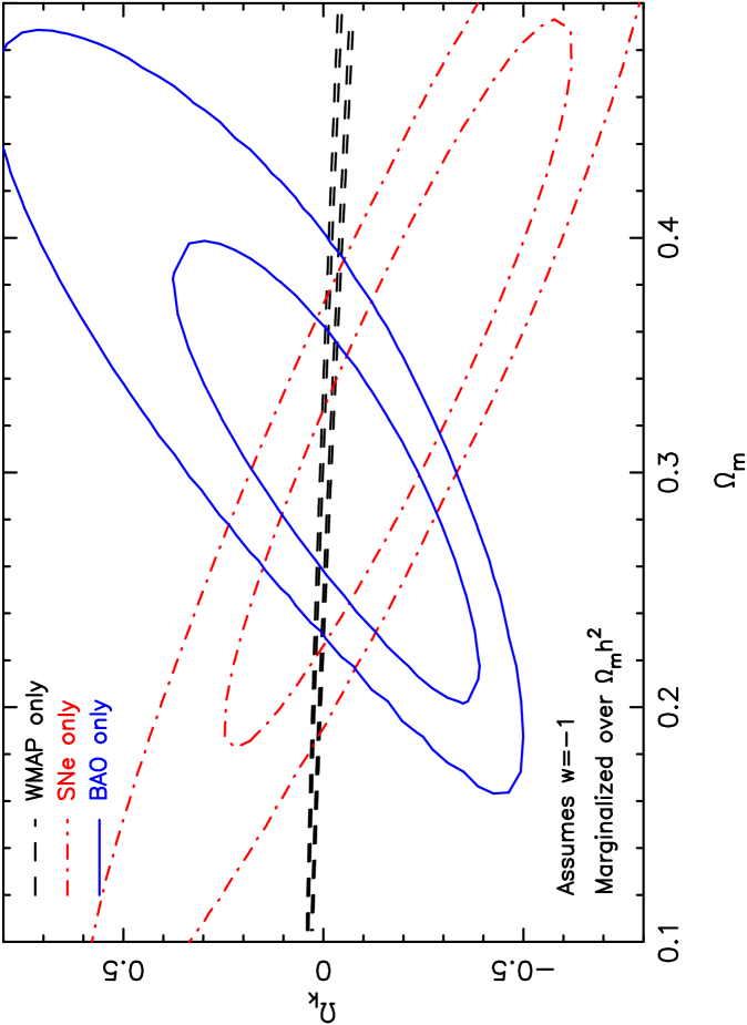
Figures 15 and 16 compare the joint probability of and , marginalizing over , for the individual WMAP, BAO and SNe datasets along with various combinations. Once more, we find that fits to WMAP+BAO and WMAP+SNe produce mutually consistent results. The BAO data has higher sensitivity to curvature because of the long lever arm represented by the relation of distance measurements at and at recombination. Combining all three datasets produces the marginalized result (errors in the other parameters are listed in Table 4). The best-fitting parameters are consistent with zero spatial curvature.

7.6 Additional degrees of freedom
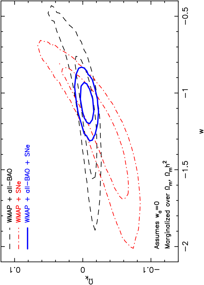
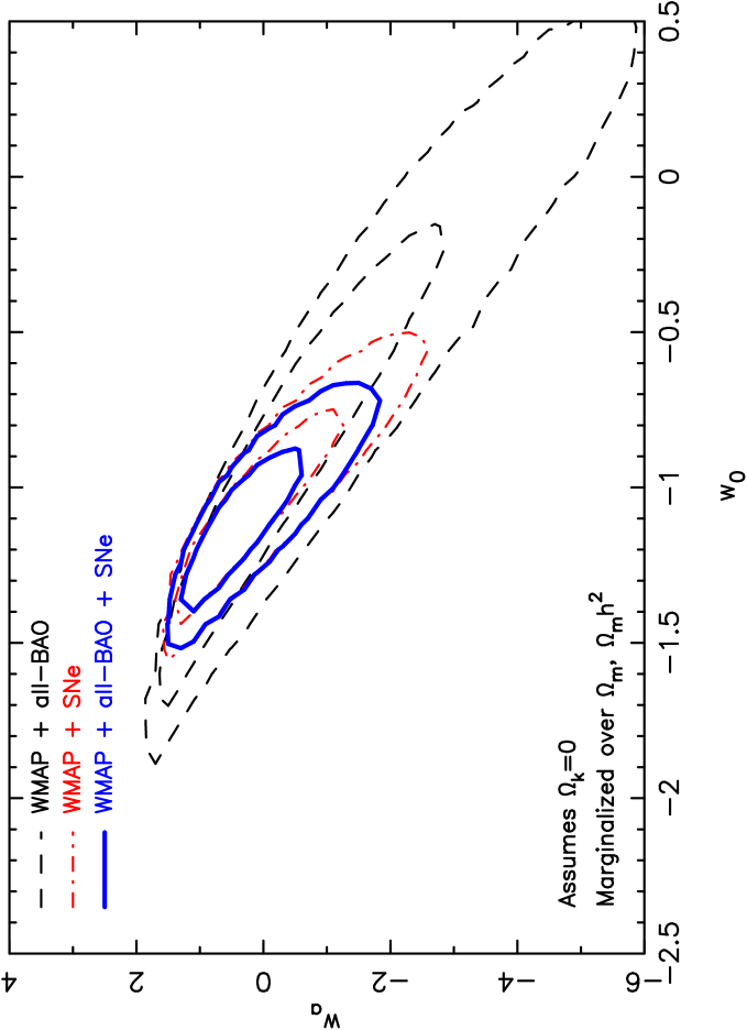
We fitted two further cosmological models, each containing an additional parameter. Firstly we fitted a curved CDM model in which we varied both the dark energy equation-of-state and the spatial curvature as free parameters. The best-fitting model has for 562 degrees of freedom, representing an improvement of compared to the case where , for the addition of a single extra parameter. In terms of information criteria this does not represent a sufficient improvement to justify the addition of the extra degree of freedom. Figure 17 compares the joint probability of and , marginalizing over and , for the three cases WMAP+BAO, WMAP+SNe and WMAP+BAO+SNe. Combining all three datasets produces the marginalized measurements and .
We finally fitted a flat CDM cosmological model in which spatial curvature is fixed at but the equation-of-state of dark energy is allowed to vary with scale factor in accordance with the Chevallier-Polarski-Linder parameterization (Chevallier & Polarski 2001, Linder 2003). The best-fitting model has for 562 degrees of freedom, and again the improvement in the value of compared to the case where does not justify the addition of the extra degree of freedom. Combining all three datasets produces the marginalized measurements and . We note that the addition of the BAO measurements to the WMAP+SNe dataset produces a more significant improvement for fits involving than for .
In all cases, the best-fitting parameters are consistent with a flat cosmological constant model for which , and . The best-fitting values and errors in the parameters for the various models, for the fits using all three datasets, are listed in Table 4.
| Model | d.o.f. | |||||||
|---|---|---|---|---|---|---|---|---|
| Flat CDM | - | - | - | |||||
| Flat CDM | - | - | ||||||
| Curved CDM | - | - | ||||||
| Curved CDM | - | |||||||
| Flat CDM | - |
8 Conclusions
We summarize the results of our study as follows:
-
•
The final dataset of the WiggleZ Dark Energy Survey allows the imprint of the baryon acoustic peak to be detected in the galaxy correlation function for independent redshift slices of width . A simple quasi-linear acoustic peak model provides a good fit to the correlation functions over a range of separations Mpc. The resulting distance-scale measurements are determined by both the acoustic peak position and the overall shape of the clustering pattern, such that the whole correlation function is being used as a standard ruler. As such, the acoustic parameter introduced by Eisenstein et al. (2005) represents the most appropriate distilled parameter for quantifying the WiggleZ BAO measurements, and we present in Table 2 a covariance matrix describing the determination of from WiggleZ data at the three redshifts , and . We test for systematics in this measurement by varying the fitting range and implementation of the quasi-linear model, and also by repeating our fits for a dark matter halo subset of the Gigaparsec WiggleZ simulation. In no case do we find evidence for significant systematic error.
-
•
We present a new measurement of the baryon acoustic feature in the correlation function of the Sloan Digital Sky Survey Luminous Red Galaxy (SDSS-LRG) sample, finding that the feature is detected within a subset spanning the redshift range with a statistical significance of -. We derive a measurement of the distilled parameter that is consistent with previous analyses of the LRG power spectrum.
-
•
We combine the galaxy correlation functions measured from the WiggleZ, 6-degree Field Galaxy Survey and SDSS-LRG samples. Each of these datasets shows independent evidence for the baryon acoustic peak, and the combined correlation function contains a BAO detection with a statistical significance of - relative to a zero-baryon model with no peak.
-
•
We fit cosmological models to the combined 6dFGS, SDSS and WiggleZ BAO dataset, now comprising six distance-redshift data points, and compare the results to similar fits to the latest compilation of supernovae (SNe) and Cosmic Microwave Background (CMB) data. The BAO and SNe datasets produce consistent measurements of the equation-of-state of dark energy, when separately combined with the CMB, providing a powerful check for systematic errors in either of these distance probes. Combining all datasets, we determine for a flat Universe, and for a curved, cosmological-constant Universe.
-
•
Adding extra degrees of freedom always produces best-fitting parameters consistent with a cosmological constant dark-energy model within a spatially-flat Universe. Varying both curvature and , we find marginalized errors and . For a dark-energy model evolving with scale factor such that , we find that and .
In conclusion, we have presented and analyzed the most comprehensive baryon acoustic oscillation dataset assembled to date. Results from the WiggleZ Dark Energy Survey have allowed us to extend this dataset up to redshift , thereby spanning the whole redshift range for which dark energy is hypothesized to govern the cosmic expansion history. By fitting cosmological models to this dataset we have established that a flat CDM cosmological model continues to provide a good and self-consistent description of CMB, BAO and SNe data. In particular, the BAO and SNe yield consistent measurements of the distance-redshift relation across the common redshift interval probed. Our results serve as a baseline for the analysis of future CMB datasets provided by the Planck satellite (Ade et al. 2011) and BAO measurements from the Baryon Oscillation Spectroscopic Survey (Eisenstein et al. 2011).
Acknowledgments
We thank the anonymous referee for careful and constructive comments that improved this study.
We acknowledge financial support from the Australian Research Council through Discovery Project grants DP0772084 and DP1093738 funding the positions of SB, DP, MP, GP and TMD. SC and DC acknowledge the support of the Australian Research Council through QEII Fellowships. MJD thanks the Gregg Thompson Dark Energy Travel Fund for financial support.
We thank the LasDamas project for making their mock catalogues publicly available. In particular EK is much obliged to Cameron McBride for supplying mock catalogues on demand. EK also thanks Ariel Sánchez for fruitful lengthy discussions. EK was partially supported by a Google Research Award and NASA Award.
FB is supported by the Australian Government through the International Postgraduate Research Scholarship (IPRS) and by scholarships from ICRAR and the AAO.
GALEX (the Galaxy Evolution Explorer) is a NASA Small Explorer, launched in April 2003. We gratefully acknowledge NASA’s support for construction, operation and science analysis for the GALEX mission, developed in co-operation with the Centre National d’Etudes Spatiales of France and the Korean Ministry of Science and Technology.
Finally, the WiggleZ survey would not be possible without the dedicated work of the staff of the Australian Astronomical Observatory in the development and support of the AAOmega spectrograph, and the running of the AAT.
References
- [1] Ade P., et al., 2011, A&A accepted (arXiv:1101.2022)
- [2] Amanullah R., et al., 2010, ApJ, 716, 712
- [3] Astier P., et al., 2006, A&A, 447, 31
- [4] Bardeen J.M., Bond J.R., Kaiser N., Szalay A.S., 1986, ApJ, 304, 15
- [5] Bassett B., Afshordi N., 2010 (arXiv:1005.1664)
- [6] Berlind A.A., Weinberg D.H., 2002, ApJ, 575, 587
- [7] Beutler F., et al., 2011, MNRAS accepted (arXiv:1106.3366)
- [8] Blake C.A, Glazebrook K., 2003, ApJ, 594, 665
- [9] Blake C.A., Parkinson D., Bassett B., Glazebrook K., Kunz M., Nichol R.C., 2006, MNRAS, 365, 255
- [10] Blake C.A., Collister A., Bridle S., Lahav O., 2007, MNRAS, 374, 1527
- [11] Blake C.A., et al., 2011, MNRAS accepted (arXiv:1105.2862)
- [12] Bond J.R., Efstathiou G., 1984, ApJ, 285, L45
- [13] Bridle S.L., Crittenden R., Melchiorri A., Hobson M.P., Kneissl R., Lasenby A.N., 2002, MNRAS, 335, 1193
- [14] Cabre A., Gaztanaga E., 2011, MNRAS, 412, 98
- [15] Chevallier M., Polarski D., 2001, Int. J. Mod. Phys., D10, 213
- [16] Cole S., et al., 2005, MNRAS, 362, 505
- [17] Cooray A., Hu W., Huterer D., Joffre M., 2001, ApJ, 557L, 7
- [18] Copin Y., et al., 2006, New Astronomy Review, 50, 436
- [19] Crocce M., Scoccimarro R., 2008, PRD, 2008, 77, 3533
- [20] Crocce M., Gaztanaga E., Cabre A., Carnero E., Sánchez E., 2011, MNRAS accepted (arXiv:1104.5236)
- [21] Dawson K.S., et al., 2009, AJ, 138, 1271
- [22] Drinkwater M., et al., 2010, MNRAS, 401, 1429
- [23] Efstathiou G., Sutherland W., Maddox S., 1990, Nature, 348, 705
- [24] Eisenstein D.J., Hu W., 1998, ApJ, 496, 605
- [25] Eisenstein D.J., Hu W., Tegmark M., 1998, ApJ, 504, 57
- [26] Eisenstein D.J., et al., 2001, AJ, 122, 2267
- [27] Eisenstein D.J., 2003, “Large-scale structure and future surveys” in “Next Generation Wide-Field Multi-Object Spectroscopy”, ASP Conference Series vol. 280, ed. M.Brown & A.Dey (astro-ph/0301623)
- [28] Eisenstein D.J., et al., 2005, ApJ, 633, 560
- [29] Eisenstein D.J., Seo H.-J., White M., 2007, ApJ, 664, 660
- [30] Eisenstein D.J. et al., 2011, AJ submitted (arXiv:1101.1529)
- [31] Fukugita M., Ichikawa T., Gunn J.E., Doi M., Shimasaku K., Schneider D.P. 1996, AJ, 111, 1748
- [32] Gilbank D.G., Gladders M.G., Yee H.K.C., Hsieh B.C., 2011, AJ, 141, 94
- [33] Glazebrook K., Blake C.A., 2005, ApJ, 631, 1
- [34] Goliath M., Amanullah R., Astier P., Goobar A., Pain R., 2001, A&A, 380, 6
- [35] Gunn J.E., et al., 1998, AJ, 116, 3040
- [36] Gunn J.E., et al., 2006, AJ, 131, 2332
- [37] Hamuy M., et al., 1996, AJ, 112, 2408
- [38] Hamuy M., et al., 2006, PASP, 118, 2
- [39] Hicken M., et al., 2009, ApJ, 700, 331
- [40] Hogg D.W., Finkbeiner D.P., Schlegel D.J., Gunn J.E., 2001, AJ, 122, 2129
- [41] Holtzman J.A., 1989, ApJS, 71, 1
- [42] Holtzman J.A., et al. 2008, AJ, 136, 2306
- [43] Hu W., Haiman Z., 2003, PRD, 68, 063004
- [44] Hu W., Sugiyama N., 1996, ApJ, 471, 542
- [45] Hutsi G., 2006, A&A, 449, 891
- [46] Ivezic Z., et al., 2004, Astronomische Nachrichten, 325, 583
- [47] Jarrett T., Chester T., Cutri R., Schneider S., Strutskie M., Huchra J.P., 2000, AJ, 119, 2498
- [48] Jha S., et al., 2006, AJ, 131, 527
- [49] Jones D.H., et al., 2009, MNRAS, 399, 683
- [50] Kaiser N., 1987, MNRAS, 227, 1
- [51] Kazin E.A., et al., 2010a, ApJ, 710, 1444
- [52] Kazin E.A., Blanton M.R., Scoccimarro R., McBride C.K., Berlind A.A., 2010b, ApJ, 719, 1032
- [53] Kazin E.A., Sánchez A.G., Blanton M.R., 2011, MNRAS submitted (arXiv:1105.2037)
- [54] Kessler R., et al., 2009, ApJS, 185, 32
- [55] Komatsu E., et al., 2009, ApJS, 180, 330
- [56] Komatsu E., et al., 2011, ApJS, 192, 18
- [57] Kowalski M., et al., 2008, ApJ, 686, 749
- [58] Krauss L.M., Turner M.S., 1996, GReGr, 27, 1137
- [59] Landy S.D., Szalay A.S., 1993, ApJ, 412, 64
- [60] Law N., et al., 2009, PASP, 121, 1395
- [61] Lewis A., Challinor A., Lasenby A., 2000, ApJ, 538, 473
- [62] Linder E.V., 2003, PRL, 90, 091301
- [63] Lupton R., Gunn J.E., Ivezic Z., Knapp G.R., Kent S., 2001, in Astronomical Society of the Pacific Conference Series, Vol. 238, Astronomical Data Analysis Software and Systems X, ed. F.R. Harnden, Jr., F.A. Primini, & H.E. Payne, 269–278
- [64] Martin D., et al., 2005, ApJ, 619, L1
- [65] Matsubara T., 2008, PRD, 78, 083519
- [66] McBride C., et al., in preparation
- [67] Miller C.J., Nichol R.C., Batuski D.J., 2001, ApJ, 555, 68
- [68] Ostriker J., Steinhardt P., 1995, Nature, 377, 600
- [69] Padmanabhan N. et al., 2007, MNRAS, 378, 852
- [70] Padmanabhan N., White M., 2008, PhRvD, 77, 3540
- [71] Padmanabhan N., White M., 2009, PhRvD, 80, 63508
- [72] Peebles P.J.E., Yu J.T., 1970, ApJ, 162, 815
- [73] Percival W.J., et al., 2001, MNRAS, 327, 1297
- [74] Percival W.J., et al., 2007, ApJ, 657, 51
- [75] Percival W.J., et al., 2010, MNRAS, 401, 2148
- [76] Perlmutter S., et al., 1999, ApJ, 517, 565
- [77] Pier J.R., Munn J.A., Hindsley R.B., Hennessy G.S., Kent S.M., Lupton R.H., Ivezic Z. 2003, AJ, 125, 1559
- [78] Poole G., et al., in preparation
- [79] Richards G., et al., 2002, AJ, 123, 2945
- [80] Riess A.G., et al., 1998, AJ, 116, 1009
- [81] Riess A.G., et al., 1999, AJ, 117, 707
- [82] Riess A.G., et al., 2004, ApJ, 607, 665
- [83] Riess A.G., et al., 2007, ApJ, 659, 98
- [84] Rimes C.D., Hamilton A.J.S., 2005, MNRAS, 360, 82
- [85] Ross A., et al., 2011, MNRAS submitted (arXiv:1105.2320)
- [86] Sánchez A.G., Baugh C.M., Angulo R., 2008, MNRAS, 390, 1470
- [87] Sánchez A.G., Crocce M., Cabre A., Baugh C.M., Gaztanaga E., 2009, MNRAS, 400, 1643
- [88] Saunders et al., 2004, SPIE, 5492, 389
- [89] Seo H.-J., Eisenstein D.J., 2003, ApJ, 598, 720
- [90] Seo H.-J., Siegel E.R., Eisenstein D.J., White M., 2008, ApJ, 686, 13
- [91] Sharp et al., 2006, SPIE, 6269, 14
- [92] Shoji M., Jeong D., Komatsu E., 2009, ApJ, 693, 1404
- [93] Smith J.A., et al., 2002, AJ, 123, 2121
- [94] Smith R.E., et al., 2003, MNRAS, 341, 1311
- [95] Smith R.E., Scoccimarro R., Sheth R., 2008, PhRvD, 77, 43525
- [96] Stoughton C., et al., 2002, AJ, 123, 485
- [97] Sunyaev R.A., Zeldovitch, Y.B., 1970, Ap&SS, 7, 3
- [98] Takahashi R., et al., 2011, ApJ, 726, 7
- [99] Taruya A., Nishimichi T., Saito S., 2010, PRD, 82, 3522
- [100] Tegmark M., 1997, PRL, 79, 20
- [101] Thomas S., Abdalla F., Lahav O., 2011, PhRvL, 106, 1301
- [102] Tucker D.L., et al., 2006, Astronomische Nachrichten, 327, 821
- [103] White M., et al., 2011, ApJ, 728, 126
- [104] Wood-Vasey W.M., et al., 2007, ApJ, 666, 694
- [105] York D.G. et al., 2000, AJ, 120, 1579