Compressive Imaging using Approximate Message Passing and a Markov-Tree Prior

Abstract

We propose a novel algorithm for compressive imaging that exploits both the sparsity and persistence across scales found in the 2D wavelet transform coefficients of natural images. Like other recent works, we model wavelet structure using a hidden Markov tree (HMT) but, unlike other works, ours is based on loopy belief propagation (LBP). For LBP, we adopt a recently proposed “turbo” message passing schedule that alternates between exploitation of HMT structure and exploitation of compressive-measurement structure. For the latter, we leverage Donoho, Maleki, and Montanari’s recently proposed approximate message passing (AMP) algorithm. Experiments with a large image database suggest that, relative to existing schemes, our turbo LBP approach yields state-of-the-art reconstruction performance with substantial reduction in complexity.

I Introduction

In compressive imaging [1], we aim to estimate an image $\boldsymbol{x}\in\mathbb{R}^{N}$ from $M\leq N$ noisy linear observations $\boldsymbol{y}\in\mathbb{R}^{M}$,

$$\boldsymbol{y} = \boldsymbol{\Phi x}+\boldsymbol{w}\,=\,\boldsymbol{\Phi\Psi\theta}+\boldsymbol{w},$$ (1)

assuming that the image has a representation $\boldsymbol{\theta}\in{\mathbb{R}}^{N}$ in some wavelet basis $\boldsymbol{\Psi}$ (i.e., $\boldsymbol{x}=\boldsymbol{\Psi\theta}$) containing only a few ($K$) large coefficients (i.e., $K\ll N$). In (1), $\boldsymbol{\Phi}\in\mathbb{R}^{M\times N}$ is a known measurement matrix and $\boldsymbol{w}\sim\mathcal{N}(\boldsymbol{0},\sigma^{2}\boldsymbol{I})$ is additive white Gaussian noise. Though $M\!<\!N$ makes the problem ill-posed, it has been shown that $\boldsymbol{x}$ can be recovered from $\boldsymbol{y}$ when $K$ is adequately small and $\boldsymbol{\Phi}$ is incoherent with $\boldsymbol{\Psi}$ [1]. The wavelet coefficients of natural images are known to have an additional structure known as persistence across scales (PAS) [2], which we now describe. For 2D images, the wavelet coefficients are naturally organized into quad-trees, where each coefficient at level $j$ acts as a parent for four child coefficients at level $j\!+\!1$. The PAS property says that, if a parent is very small, then all of its children are likely to be very small; similarly, if a parent is large, then it is likely that some (but not necessarily all) of its children will also be large.

Several authors have exploited the PAS property for compressive imaging [3, 4, 5, 6]. The so-called “model-based” approach [3] is a deterministic incarnation of PAS that leverages a restricted union-of-subspaces and manifests as a modified CoSaMP [7] algorithm. Most approaches are Bayesian in nature, exploiting the fact that PAS is readily modeled by a hidden Markov tree (HMT) [8]. The first work in this direction appears to be [4], where an iteratively re-weighted $\ell_{1}$ algorithm, generating an estimate of $\boldsymbol{x}$, was alternated with a Viterbi algorithm, generating an estimate of the HMT states. More recently, HMT-based compressive imaging has been attacked using modern Bayesian tools [9]. For example, [5] used Markov-chain Monte-Carlo (MCMC), which is known to yield correct posteriors after convergence. For practical image sizes, however, convergence takes an impractically long time, and so MCMC must be terminated early, at which point its performance may suffer. Variational Bayes (VB) can sometimes offer a better performance/complexity tradeoff, motivating the approach in [6]. Our experiments indicate that, while [6] indeed offers a good performance/complexity tradeoff, it is possible to do significantly better.

In this paper, we propose a novel approach to HMT-based compressive imaging based on loopy belief propagation [10]. For this, we model the coefficients in $\boldsymbol{\theta}$ as conditionally Gaussian with variances that depend on the values of HMT states, and we propagate beliefs (about both coefficients and states) on the corresponding factor graph. A recently proposed “turbo” messaging schedule [11] suggests to iterate between exploitation of HMT structure and exploitation of observation structure from (1). For the former we use the standard sum-product algorithm [12, 13], and for the latter we use the recently proposed approximate message passing (AMP) approach [14]. The remarkable properties of AMP are 1) a rigorous analysis (as $M,N\rightarrow\infty$ with $M/N$ fixed, under i.i.d Gaussian $\boldsymbol{\Phi}$) [15] establishing that its solutions are governed by a state-evolution whose fixed points—when unique—yield the true posterior means, and 2) very low implementational complexity (e.g., AMP requires one forward and one inverse fast-wavelet-transform per iteration, and very few iterations).

We consider two types of conditional-Gaussian coefficient models: a Bernoulli-Gaussian (BG) model and a two-state Gaussian-mixture (GM) model. The BG model assumes that the coefficients are either generated from a large-variance Gaussian distribution or are exactly zero (i.e., the coefficients are exactly sparse), whereas the GM model assumes that the coefficients are generated from either a large-variance or a small-variance Gaussian distribution. Both models have been previously applied for imaging, e.g., the BG model was used in [6, 5], whereas the GM model was used in [8, 4].

Although our models for the coefficients $\boldsymbol{\theta}$ and the corresponding HMT states involve statistical parameters like variance and transition probability, we learn those parameters directly from the data. To do so, we take a hierarchical Bayesian approach—similar to [6, 5]—where these statistical parameters are treated as random variables with suitable hyperpriors. Experiments on a large image database show that our turbo-AMP approach yields state-of-the-art reconstruction performance with substantial reduction in complexity.

The remainder of the paper is organized as follows. Section II describes the signal model, Section III describes the proposed algorithm, Section IV gives numerical results and comparisons with other algorithms, and Section V concludes.

Notation: Above and in the sequel, we use lowercase boldface quantities to denote vectors, uppercase boldface quantities to denote matrices, $\boldsymbol{I}$ to denote the identity matrix, $(\cdot)^{T}$ to denote transpose, and $\|\boldsymbol{x}\|_{2}\triangleq\sqrt{\boldsymbol{x}^{T}\boldsymbol{x}}$. We use $p_{\Theta|S}(\theta\,|\,s)$ to denote the probability density function (pdf) of random variable $\Theta$ given the event $S=s$, where often the subscript “$\mbox{}_{\Theta|S}$” is omitted when there is no danger of confusion. We use $\mathcal{N}(\boldsymbol{x};\boldsymbol{m},\boldsymbol{\Sigma})$ to denote the $N$-dimensional Gaussian pdf with argument $\boldsymbol{x}$, mean $\boldsymbol{m}$, and covariance matrix $\boldsymbol{\Sigma}$, and we write $\boldsymbol{x}\sim\mathcal{N}(\boldsymbol{m},\boldsymbol{\Sigma})$ to indicate that random vector $\boldsymbol{x}$ has this pdf. We use $\operatorname{E}\{\cdot\}$ to denote expectation, $\Pr\{\mathcal{E}\}$ to denote the probability of event $\mathcal{E}$, and $\delta(\cdot)$ to denote the Dirac delta. Finally, we use $\propto$ to denote equality up to a multiplicative constant.

II Signal Model

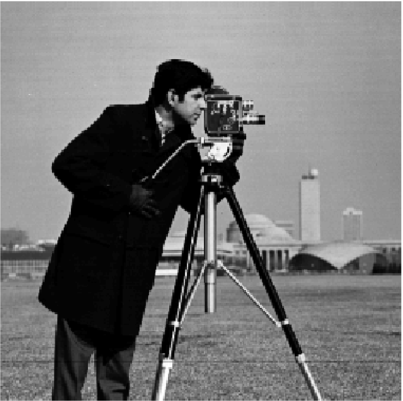
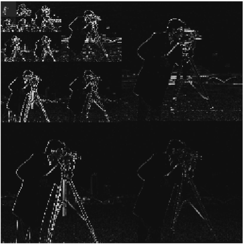
Figure 1: Left: The camera-man image. Center: The corresponding transform coefficients, demonstrating PAS. Right: An illustration of quad-tree structure.

Throughout, we assume that $\boldsymbol{\Psi}$ represents a 2D wavelet transform [2], so that the transform coefficients $\boldsymbol{\theta}=[\theta_{1},\dots,\theta_{N}]^{T}$ can be partitioned into so-called “wavelet” coefficients (at indices $n\in\mathcal{W}$) and “approximation” coefficients (at indices $n\in\mathcal{A}$). The wavelet coefficients can be further partitioned into several quad-trees, each with $J\geq 1$ levels (see Fig. 1). We denote the indices of all coefficients at level $j\in\{0,\dots,J\!-\!1\}$ of these wavelet trees by $\mathcal{W}_{j}$, where $j=0$ refers to the root. In the interest of brevity, and with a slight abuse of notation, we refer to the approximation coefficients as level “$-1$” of the wavelet tree (i.e., $\mathcal{A}=\mathcal{W}_{-1}$).

As discussed earlier, two coefficient models are considered in this paper: Bernoulli-Gaussian (BG) and two-state Gaussian mixture (GM). For ease of exposition, we focus on the BG model until Section III-E, at which point the GM case is detailed. In the BG model, each transform coefficient $\theta_{n}$ is modeled using the (conditionally independent) prior pdf

$$p(\theta_{n}\,|\,s_{n}) = s_{n}\mathcal{N}(\theta_{n};0,\sigma_{n}^{2})+(1-s_{n})\delta(\theta_{n}),$$ (2)

where $s_{n}\in\{0,1\}$ is a hidden binary state. The approximation states $\{s_{n}\}_{n\in\mathcal{W}_{-1}}$ are assigned the apriori activity rate $\pi_{-1}^{1}\triangleq\Pr\{s_{n}\!=\!1\,|\,n\in\mathcal{W}_{-1}\}$, which is discussed further below. Meanwhile, the root wavelet states $\{s_{n}\}_{n\in\mathcal{W}_{0}}$ are assigned $\pi_{0}^{1}\triangleq\Pr\{s_{n}\!=\!1\,|\,n\in\mathcal{W}_{0}\}$. Within each quad-tree, the states have a Markov structure. In particular, the activity of a state at level $j+1$ is determined by its parent’s activity (at level $j$) and the transition probabilities $\{\pi_{j}^{00},\pi_{j}^{11}\}$, where $\pi_{j}^{00}$ denotes the probability that the child’s state equals $0$ given that his parent’s state also equals $0$, and $\pi_{j}^{11}$ denotes the probability that the child’s state equals $1$ given given that his parent’s state also equals $1$. The corresponding factor graph is shown in Fig. 2.

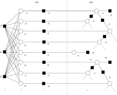
Figure 2: Factor graph representation of the signal model. The variables $s_{1}$ and $s_{6}$ are wavelet states at the roots of two different Markov trees. The variable $s_{5}$ is an approximation state and hence is not part of any Markov tree. The remaining $s_{n}$ are wavelet states at levels $j>0$. For visual simplicity, a binary-tree is shown instead of a quad-tree, and the nodes representing the statistical parameters $\rho,\pi_{-1}^{1},\pi_{0}^{1},\{\rho_{j},\pi_{j}^{11},\pi_{j}^{00}\}$, as well as those representing their hyperpriors, are not shown.

We take a hierarchical Bayesian approach, modeling the statistical parameters $\sigma^{2},\{\sigma_{n}^{2}\}_{n=1}^{N},\pi_{-1}^{1},\pi_{0}^{1},\{\pi_{j}^{11},\pi_{j}^{00}\}_{j=0}^{J-2}$ as random variables and assigning them appropriate hyperpriors. Rather than working directly with variances, we find it more convenient to work with precisions (i.e., inverse-variances) such as $\rho\triangleq\sigma^{-2}$. We then assume that all coefficients at the same level have the same precision, so that $\rho_{j}=\sigma_{n}^{-2}$ for all $n\in\mathcal{W}_{j}$. To these precisions, we assign conjugate priors [16], which in this case take the form

$$\rho \sim \mathrm{Gamma}(a,b)$$ (3)

$$\rho_{j} \sim \mathrm{Gamma}(a_{j},b_{j}),$$ (4)

where $\mathrm{Gamma}(\rho;a,b)\triangleq\frac{1}{\Gamma(a)}b^{a}\rho^{a-1}\exp(-b\rho)$ for $\rho\geq 0$, and where $a,b,\{a_{j},b_{j}\}_{j=-1}^{J-1}$ are hyperparameters. (Recall that the mean and variance of $\mathrm{Gamma}(a,b)$ are given by $a/b$ and $a/b^{2}$, respectively [16].) For the activity rates and transition parameters, we assume

$$\pi_{0}^{1} \sim \mathrm{Beta}(c,d)$$ (5)

$$\pi_{-1}^{1} \sim \mathrm{Beta}(\underline{c},\underline{d})$$ (6)

$$\pi_{j}^{11} \sim \mathrm{Beta}(c_{j},d_{j})$$ (7)

$$\pi_{j}^{00} \sim \mathrm{Beta}(\underline{c}_{j},\underline{d}_{j}),$$ (8)

where $\mathrm{Beta}(p;c,d)\triangleq\frac{\Gamma(c+d)}{\Gamma(c)\Gamma(d)}p^{c-1}(1-p)^{d-1}$, and where $c,d,\underline{c},\underline{d},\{c_{j},d_{j},\underline{c}_{j},\underline{d}_{j}\}_{j=1}^{J-1}$ are hyperparameters. (Recall that the mean and variance of $\mathrm{Beta}(c,d)$ are given by $\frac{c}{c+d}$ and $\frac{cd}{(c+d)^{2}(c+d+1)}$, respectively [16].) Our hyperparameter choices are detailed in Section IV.

III Image Reconstruction

To infer the wavelet coefficients $\boldsymbol{\theta}$, we would ideally like to compute the posterior pdf

$$p(\boldsymbol{\theta}\,|\,\boldsymbol{y}) \propto \sum_{\boldsymbol{s}}p(\boldsymbol{y}\,|\,\boldsymbol{\theta},\boldsymbol{s})p(\boldsymbol{\theta},\boldsymbol{s})$$ (9)

$$= \sum_{\boldsymbol{s}}\underbrace{p(\boldsymbol{s})}_{\displaystyle\triangleq h(\boldsymbol{s})}\prod_{n=1}^{N}\underbrace{p(\theta_{n}\,|\,s_{n})}_{\displaystyle\triangleq f_{n}(\theta_{n},s_{n})}\prod_{m=1}^{M}\underbrace{p(y_{m}\,|\,\boldsymbol{\theta})}_{\displaystyle\triangleq g_{m}(\boldsymbol{\theta})},\quad$$ (10)

where $\propto$ denotes equality up to a multiplicative constant. For the BG coefficient model, $f_{n}(\theta_{n},s_{n})$ is specified by (2). Due to the white Gaussian noise model (1), we have $g_{m}(\boldsymbol{\theta})=\mathcal{N}(y_{m};\boldsymbol{a}_{m}^{T}\boldsymbol{\theta},\sigma^{2})$, where $\boldsymbol{a}_{m}^{T}$ denotes the $m^{\mathrm{th}}$ row of the matrix $\boldsymbol{A}\triangleq\boldsymbol{\Phi\Psi}$.

III-A Loopy Belief Propagation

While exact computation of $p(\boldsymbol{\theta}\,|\,\boldsymbol{y})$ is computationally prohibitive, the marginal posteriors $\{p(\theta_{n}\,|\,\boldsymbol{y})\}$ can be efficiently approximated using loopy belief propagation (LBP) [10] on the factor graph of Fig. 2, which uses round nodes to denote variables and square nodes to denote the factors in (10). In doing so, we also obtain the marginal posteriors $\{p(s_{n}\,|\,\boldsymbol{y})\}$. For now, we treat statistical parameters $\rho,\pi_{-1}^{1},\pi_{0}^{1},\{\rho_{j},\pi_{j}^{11},\pi_{j}^{00}\}$, as if they were fixed and known, and we detail the procedure by which they are learned in Section III-D.

In LBP, messages are exchanged between the nodes of the factor graph until they converge. Messages take the form of pdfs (or pmfs), and the message flowing to/from a variable node can be interpreted as a local belief about that variable. According to the sum-product algorithm [12, 13] the message emitted by a variable node along a given edge is (an appropriate scaling of) the product of the incoming messages on all other edges. Meanwhile, the message emitted by a function node along a given edge is (an appropriate scaling of) the integral (or sum) of the product of the node’s constraint function and the incoming messages on all other edges, where the integration (or summation) is performed over all variables other than the one directly connected to the edge along which the message travels. When the factor graph has no loops, exact marginal posteriors result from two (i.e., forward and backward) passes of the sum-product algorithm [12, 13]. When the factor graph has loops, however, exact inference is known to be NP hard [17] and so LBP is not guaranteed to produce correct posteriors. Still, LBP has shown state-of-the-art performance in many applications, such as inference on Markov random fields [18], turbo decoding [19], LDPC decoding [20], multiuser detection [21], and compressive sensing [22, 14, 23, 15].

III-B Message Scheduling: The Turbo Approach

With loopy belief propagation, there exists some freedom in how messages are scheduled. In this work, we adopt the “turbo” approach recently proposed in [11]. For this, we split the factor graph in Fig. 2 along the dashed line and obtain the two decoupled subgraphs in Fig. 3. We then alternate between belief propagation on each of these two subgraphs, treating the likelihoods on $\{s_{n}\}$ generated from belief propagation on one subgraph as priors for subsequent belief propagation on the other subgraph. We now give a more precise description of this turbo scheme, referring to one full round of alternation as a “turbo iteration.” In the sequel, we use $\nu_{A\to B}^{\scriptscriptstyle(t)}(.)$ to denote the message passed from node $A$ to node $B$ during the $t^{\mathrm{th}}$ turbo iteration.

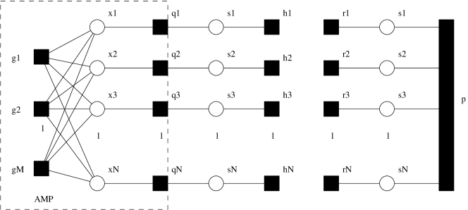
Figure 3: The turbo approach yields a decoupled factor graph.

The procedure starts at $t=1$ by setting the “prior” pmfs $\{h_{n}^{\scriptscriptstyle(1)}(.)\}$ in accordance with the apriori activity rates $\Pr\{s_{n}=1\}$ described in Section II. LBP is then iterated (to convergence) on the left subgraph in Fig. 3, finally yielding the messages $\{\nu_{f_{n}\to s_{n}}^{\scriptscriptstyle(1)}(.)\}$. We note that the message $\nu_{f_{n}\to s_{n}}^{\scriptscriptstyle(1)}(s_{n})$ can be interpreted as the current estimate of the likelihood on $s_{n}$, i.e., $p(\boldsymbol{y}\,|\,s_{n})$ as a function of $s_{n}$. These likelihoods are then treated as priors for belief propagation on the right subgraph, as facilitated by the assignment $d_{n}^{\scriptscriptstyle(1)}(.)=\nu_{f_{n}\to s_{n}}^{\scriptscriptstyle(1)}(.)$ for each $n$. Due to the tree structure of HMT, there are no loops in right subgraph (i.e., inside the “$h$” super-node in Fig. 3), and thus it suffices to perform only one forward-backward pass of the sum-product algorithm [12, 13]. The resulting leftward messages $\nu_{h\to s_{n}}^{(1)}(.)$ are subsequently treated as priors for belief propagation on the left subgraph at the next turbo iteration, as facilitated by the assignment $h_{n}^{(2)}(.)=\nu_{h\to s_{n}}^{(1)}(.)$. The process then continues for turbo iterations $t=2,3,4,\dots$, until the likelihoods converge or a maximum number of turbo iterations has elapsed. Formally, the turbo schedule is summarized by

$$d_{n}^{(t)}(s_{n}) = \nu_{f_{n}\to s_{n}}^{(t)}(s_{n})$$ (11)

$$h_{n}^{(t+1)}(s_{n}) = \nu_{h\to s_{n}}^{(t)}(s_{n}).$$ (12)

In the sequel, we refer to inference of $\{s_{n}\}$ using compressive-measurement structure (i.e., inference on the left subgraph of Fig. 3) as soft support-recovery (SSR) and inference of $\{s_{n}\}$ using HMT structure (i.e., inference on the right subgraph of Fig. 3) as soft support-decoding (SSD). SSR details are described in the next subsection.

III-C Soft Support-Recovery via AMP

We now discuss our implementation of SSR during a single turbo iteration $t$. Because the operations are invariant to $t$, we suppress the $t$-notation. As described above, SSR performs several iterations of loopy belief propagation per turbo iteration using the fixed priors $\lambda_{n}\triangleq h_{n}(s_{n}=1)$. This implies that, over SSR’s LBP iterations, the message $\nu_{f_{n}\to\theta_{n}}(.)$ is fixed at

$$\nu_{f_{n}\to\theta_{n}}(\theta_{n}) = \lambda_{n}\mathcal{N}(\theta_{n};0,\sigma_{n}^{2})+(1-\lambda_{n})\delta(\theta_{n}).$$ (13)

The dashed box in Fig. 3 shows the region of the factor graph on which messages are updated during SSR’s LBP iterations. This subgraph can be recognized as the one that Donoho, Maleki, and Montanari used to derive their so-called approximate message passing (AMP) algorithm [14]. While [14] assumed an i.i.d Laplacian prior for $\boldsymbol{\theta}$, the approach for generic i.i.d priors was outlined in [23]. Below, we extend the approach of [23] to independent non-identical priors (as analyzed in [24]) and we detail the Bernoulli-Gaussian case. In the sequel, we use a superscript-$i$ to index SSR’s LBP iterations.

According to the sum-product algorithm, the fact that $\nu_{f_{n}\to\theta_{n}}(.)$ is non-Gaussian implies that $\nu^{i}_{\theta_{n}\to g_{m}}(.)$ is also non-Gaussian, which complicates the exact calculation of the subsequent messages $\nu^{i}_{g_{m}\to\theta_{n}}(.)$ as defined by the sum-product algorithm. However, for large $N$, the combined effect of $\{\nu^{i}_{\theta_{n}\to g_{m}}(.)\}_{n=1}^{N}$ at the $g_{m}$ nodes can be approximated as Gaussian using central-limit theorem (CLT) arguments, after which it becomes sufficient to parameterize each message $\nu^{i}_{\theta_{n}\to g_{m}}(.)$ by only its mean and variance:

$$\mu_{mn}^{i} \triangleq \textstyle\int_{\theta_{n}}\theta_{n}\,\nu^{i}_{\theta_{n}\to g_{m}}(\theta_{n})$$ (14)

$$v_{mn}^{i} \triangleq \textstyle\int_{\theta_{n}}(\theta_{n}-\mu^{i}_{mn})^{2}\,\nu^{i}_{\theta_{n}\to g_{m}}(\theta_{n}).$$ (15)

Combining

$$\prod_{q}\mathcal{N}(\theta;\mu_{q},v_{q}) \propto \mathcal{N}\left(\theta;\frac{\sum_{q}\mu_{q}/v_{q}}{\sum_{q}1/v_{q}},\frac{1}{\sum_{q}1/v_{q}}\right)$$ (16)

with $g_{m}(\boldsymbol{\theta})=\mathcal{N}(y_{m};\boldsymbol{a}^{T}_{m}\boldsymbol{\theta},\sigma^{2})$, the CLT then implies that

$$\nu^{i}_{g_{m}\to\theta_{n}}(\theta_{n}) \approx \mathcal{N}\left(\theta_{n};\frac{z_{mn}^{i}}{A_{mn}},\frac{c^{i}_{mn}}{A_{mn}^{2}}\right)$$ (17)

$$z^{i}_{mn} \triangleq \textstyle y_{m}-\sum_{q\neq n}A_{mq}\mu^{i}_{qm}$$ (18)

$$c^{i}_{mn} \triangleq \textstyle\sigma^{2}+\sum_{q\neq n}A_{mq}^{2}v^{i}_{qm}.$$ (19)

The updates $\mu^{i+1}_{mn}$ and $v^{i+1}_{mn}$ can then be calculated from

$$\nu^{i+1}_{\theta_{n}\to g_{m}}(\theta_{n}) \propto \textstyle\nu_{f_{n}\to\theta_{n}}(\theta_{n})\prod_{l\neq m}\nu^{i}_{g_{l}\to\theta_{n}}(\theta_{n}),$$ (20)

where, using (16), the product term in (20) is

$$\propto\mathcal{N}\left(\theta_{n};\frac{\sum_{l\neq m}A_{ln}z^{i}_{ln}/c^{i}_{ln}}{\sum_{l\neq m}A^{2}_{ln}z^{i}_{ln}/c^{i}_{ln}},\frac{1}{\sum_{l\neq m}A^{2}_{ln}/c^{i}_{ln}}\right).$$ (21)

Assuming that the values $A_{ln}^{2}$ satisfy

$$\sum_{l\neq m}A^{2}_{ln}\approx\sum_{l=1}^{M}A^{2}_{ln}\approx 1,$$ (22)

which occurs, e.g., when $M$ is large and $\{A_{ln}\}$ are generated i.i.d with variance $1/M$, we have $c^{i}_{ln}\approx\textstyle c^{i}_{n}\triangleq\frac{1}{M}\sum_{m=1}^{M}c^{i}_{mn}$, and thus (20) is well approximated by

$$\nu^{i+1}_{\theta_{n}\to g_{m}}(\theta_{n}) \propto \left(\lambda_{n}\mathcal{N}(\theta_{n};0,\sigma_{n}^{2})+(1-\lambda_{n})\delta(\theta_{n})\right)$$ (23)

$$\mbox{}\times\mathcal{N}(\theta_{n};\xi_{nm}^{i},c_{n}^{i})$$

$$\xi^{i}_{nm} \triangleq \textstyle\sum_{l\neq m}A_{ln}z^{i}_{ln}.$$ (24)

In this case, the mean and variance of $\nu^{i+1}_{\theta_{n}\to g_{m}}(.)$ become

$$\mu_{nm}^{i+1} = \alpha_{n}(c_{n}^{i})\xi_{nm}^{i}/(1+\gamma_{nm}^{i})$$ (25)

$$v_{nm}^{i+1} = \gamma_{nm}^{i}(\mu_{nm}^{i+1})^{2}+\mu_{nm}^{i+1}c_{n}^{i}/\xi_{nm}^{i}$$ (26)

$$\gamma_{nm}^{i} \triangleq \beta_{n}(c_{n}^{i})\exp(-\zeta_{n}(c_{n}^{i})(\xi_{nm}^{i})^{2}),$$ (27)

where

$$\alpha_{n}(c) \triangleq (c/\sigma_{n}^{2}+1)^{-1}$$

$$\beta_{n}(c) \triangleq (-1+1/\lambda_{n})\sqrt{1+\sigma_{n}^{2}/c}$$

$$\zeta_{n}(c) \triangleq (2c(1+c/\sigma_{n}^{2}))^{-1}.$$

According to the sum-product algorithm, $\hat{p}^{i+1}(\theta_{n}\,|\,\boldsymbol{y})$, the posterior on $\theta_{n}$ after SSR’s $i^{\mathrm{th}}$-LBP iteration, obeys

$$\hat{p}^{i+1}(\theta_{n}\,|\,\boldsymbol{y}) \propto \textstyle\nu_{f_{n}\to\theta_{n}}(\theta_{n})\prod_{l=1}^{M}\nu^{i}_{g_{l}\to\theta_{n}}(\theta_{n}),$$ (28)

whose mean and variance determine the $i^{\mathrm{th}}$-iteration MMSE estimate of $\theta_{n}$ and its variance, respectively. Noting that the difference between (28) and (20) is only the inclusion of the $m^{\mathrm{th}}$ product term, these MMSE quantities become

$$\mu_{n}^{i+1} = \alpha_{n}(c_{n}^{i})\xi_{n}^{i}/(1+\gamma_{n}^{i})$$ (29)

$$v_{n}^{i+1} = \gamma_{n}^{i}(\mu_{n}^{i+1})^{2}+\mu_{n}^{i+1}c_{n}^{i}/\xi_{n}^{i}$$ (30)

$$\xi^{i}_{n} \triangleq \textstyle\sum_{l=1}^{M}A_{ln}z^{i}_{ln}$$ (31)

$$\gamma_{n}^{i} \triangleq \beta_{n}(c_{n}^{i})\exp(-\zeta_{n}(c_{n}^{i})(\xi_{n}^{i})^{2}).$$ (32)

Similarly, the posterior on $s_{n}$ after the $i^{\mathrm{th}}$ iteration obeys

$$\hat{p}^{i+1}(s_{n}\,|\,\boldsymbol{y}) \propto \nu^{i}_{f_{n}\to s_{n}}(s_{n})\nu_{h_{n}\to s_{n}}(s_{n}),$$ (33)

where

$$\nu^{i}_{f_{n}\to s_{n}}(s_{n}) \propto \int_{\theta_{n}}f_{n}(\theta_{n},s_{n})\prod_{l=1}^{M}\nu^{i}_{g_{l}\to\theta_{n}}(\theta_{n}).$$ (34)

Since $f_{n}(\theta_{n},s_{n})=s_{n}\mathcal{N}(\theta_{n};0,\sigma_{n}^{2})+(1-s_{n})\delta(\theta_{n})$, it can be seen that the corresponding log-likelihood ratio (LLR) is

$$L^{i+1}_{n}\triangleq\ln\frac{\nu_{f_{n}\to s_{n}}^{i}(s_{n}\!=\!1)}{\nu_{f_{n}\to s_{n}}^{i}(s_{n}\!=\!0)}=\ln\frac{1-\lambda_{n}^{i}}{\gamma_{n}^{i}\lambda_{n}^{i}}.\quad$$ (35)

Clearly, the LLR $L_{n}^{i+1}$ and the likelihood function $\nu_{f_{n}\to s_{n}}^{i}(.)$ express the same information, but in different ways.

The procedure described thus far updates $\mathcal{O}(MN)$ variables per LBP iteration, which is impractical since $MN$ can be very large. In [23], Donoho, Maleki, and Montanari proposed, for the i.i.d case, further approximations that yield a “first-order” approximate message passing (AMP) algorithm that allows the update of only $\mathcal{O}(N)$ variables per LBP iteration, essentially by approximating the differences among the outgoing means/variances of the $g_{m}(\cdot)$ nodes (i.e., $z^{i}_{mn}$ and $c^{i}_{mn}$) as well as the differences among the outgoing means/variances of the $\theta_{n}$ nodes (i.e., $\mu_{n}^{i}$ and $v_{n}^{i}$). These resulting algorithm was then rigorously analyzed by Bayati and Montanari in [15]. We now summarize a straightforward extension of the i.i.d AMP algorithm from [23] to the case of an independent but non-identical Bernoulli-Gaussian prior (13):

$$\xi^{i}_{n} = \textstyle\sum_{m=1}^{M}A_{mn}z^{i}_{m}+\mu^{i}_{n}$$ (36)

$$\mu^{i+1}_{n} = F_{n}(\xi^{i}_{n};c^{i})$$ (37)

$$v^{i+1}_{n} = G_{n}(\xi^{i}_{n};c^{i})$$ (38)

$$z^{i+1}_{m} = \textstyle y_{m}-\sum_{n=1}^{N}A_{mn}\mu^{i}_{n}+\frac{z^{i}_{m}}{M}\sum_{n=1}^{N}F^{\prime}_{n}(\xi^{i}_{n};c^{i})$$ (39)

$$c^{i+1} = \textstyle\sigma^{2}+\frac{1}{M}\sum_{n=1}^{N}v^{i+1}_{n},$$ (40)

where $F_{n}(.;.)$, $G_{n}(.;.)$ and $F^{\prime}_{n}(.;.)$ are defined as

$$F_{n}(\xi;c) = \frac{\alpha_{n}(c)}{1+\tau_{n}(\xi;c)}\xi$$ (41)

$$G_{n}(\xi;c) = \tau_{n}(\xi;c)F_{n}(\xi;c)^{2}+c\,\xi^{-1}\!F_{n}(\xi;c)$$ (42)

$$F^{\prime}_{n}(\xi;c) = \frac{\alpha_{n}(c)\big{[}1+\tau_{n}(\xi;c)\left(1+2\zeta(c_{n})\xi^{2}\right)\!\!\big{]}}{[1+\tau_{n}(\xi;c)]^{2}}\!\quad$$ (43)

$$\tau_{n}(\xi;c) = \beta_{n}(c)\exp(-\zeta_{n}(c)\xi^{2}).$$ (44)

For the first turbo iteration (i.e., $t\!=\!1$), we initialize AMP using $z^{i=1}_{m}=y_{m}$, $\mu^{i=1}_{n}=0$, and $c^{i=1}_{n}\gg\sigma_{n}^{2}$ for all $m,n$. For subsequent turbo iterations (i.e., $t\!>\!1$), we initialize AMP by setting $z^{i=1}_{m},\mu^{i=1}_{n},c^{i=1}_{n}$ equal to the final values of $z^{i}_{m},\mu^{i}_{n},c^{i}_{n}$ generated by AMP at the previous turbo iteration. We terminate the AMP iterations as soon as either $\|\boldsymbol{\mu}^{i}-\boldsymbol{\mu}^{i-1}\|_{2}<10^{-5}$ or a maximum of $10$ AMP iterations have elapsed. Similarly, we terminate the turbo iterations as soon as either $\|\boldsymbol{\mu}^{\scriptscriptstyle(t)}-\boldsymbol{\mu}^{\scriptscriptstyle(t-1)}\|_{2}<10^{-5}$ a maximum of $10$ turbo iterations have elapsed. The final value of $\boldsymbol{\mu}=[\mu_{1},\dots,\mu_{N}]^{T}$ is output at the signal estimate $\hat{\boldsymbol{\theta}}$.

III-D Learning the Statistical Parameters

We now describe how the precisions $\{\rho_{j}\}$ are learned. First, we recall that $\rho_{j}$ describes the apriori precision on the active coefficients at the $j^{th}$ level, i.e., on $\{\theta_{n}\}_{n\in\mathcal{S}_{j}}$, where the corresponding index set $\mathcal{S}_{j}\triangleq\{n\in\mathcal{W}_{j}:s_{n}=1\}$ is of size $K_{j}\triangleq|\mathcal{S}_{j}|$. Furthermore, we recall that the prior on $\rho_{j}$ was chosen as in (4). Thus, if we had access to the true values $\{\theta_{n}\}_{n\in\mathcal{S}_{j}}$, then (2) implies that

$$p(\theta_{n}\,|\,n\in\mathcal{S}_{j}) = \mathcal{N}(\theta_{n};0,\rho_{j}),$$ (45)

which implies that the posterior on $\rho_{j}$ would take the form of $\mathrm{Gamma}(\hat{a}_{j},\hat{b}_{j})$ where $\hat{a}_{j}=a_{j}+\frac{1}{2}K_{j}$ and $\hat{b}_{j}=b_{j}+\frac{1}{2}\sum_{n\in\mathcal{S}_{j}}\theta_{n}^{2}$. In practice, we don’t have access to the true values $\{\theta_{n}\}_{n\in\mathcal{S}_{j}}$ nor to the set $\mathcal{S}_{j}$, and thus we propose to build surrogates from the SSR outputs. In particular, to update $\rho_{j}$ after the $t^{\mathrm{th}}$ turbo iteration, we employ

$$\mathcal{S}^{\scriptscriptstyle(t)}_{j} \triangleq \{n\in\mathcal{W}_{j}:L^{\scriptscriptstyle(t)}_{n}>0\}$$ (46)

$$K^{\scriptscriptstyle(t)}_{j} \triangleq |\mathcal{S}^{\scriptscriptstyle(t)}_{j}|,$$ (47)

and $\{\mu_{n}^{\scriptscriptstyle(t)}\}_{n\in\mathcal{S}^{\scriptscriptstyle(t)}_{j}}$, where $L^{\scriptscriptstyle(t)}_{n}$ and $\mu^{\scriptscriptstyle(t)}_{n}$ denote the final LLR on $s_{n}$ and the final MMSE estimate of $\theta_{n}$, respectively, at the $t^{\mathrm{th}}$ turbo iteration. These choices imply the hyperparameters

$$\hat{a}_{j}^{\scriptscriptstyle(t+1)} = \textstyle a_{j}+\frac{1}{2}K_{j}^{\scriptscriptstyle(t)}$$ (48)

$$\hat{b}_{j}^{\scriptscriptstyle(t+1)} = \textstyle b_{j}+\frac{1}{2}\sum_{n\in\mathcal{S}^{\scriptscriptstyle(t)}_{j}}(\mu_{n}^{\scriptscriptstyle(t)})^{2}.$$ (49)

Finally, to perform SSR at turbo iteration $t+1$, we set the variances $\{\sigma_{n}^{2}\}_{n\in\mathcal{W}_{j}}$ equal to the inverse of the expected precisions, i.e., $1/\operatorname{E}\{\rho_{j}\}=\hat{b}_{j}^{\scriptscriptstyle(t+1)}/\hat{a}_{j}^{\scriptscriptstyle(t+1)}$. The noise variance $\sigma^{2}$ is learned similarly from the SSR-estimated residual.

Next, we describe how the transition probabilities $\{\pi_{j}^{11}\}$ are learned. First, we recall that $\pi_{j}^{11}$ describes the probability that a child at level $j+1$ is active (i.e., $s_{n}=1$) given that his parent (at level $j$) is active. Furthermore, we recall that the prior on $\pi_{j}^{11}$ was chosen as in (7). Thus if we knew that there were $K_{j}$ active coefficients at level $j$, of which $C_{j}$ had active children, then the posterior on $\pi_{j}^{11}$ would take the form of $\mathrm{Beta}(\hat{c}_{j},\hat{d}_{j})$, where $\hat{c}_{j}=c_{j}+C_{j}$ and $\hat{d}_{j}=d_{j}+K_{j}-C_{j}$. In practice, we don’t have access to the true values of $K_{j}$ and $C_{j}$, and thus we build surrogates from the SSR outputs. In particular, to update $\pi_{j}^{11}$ after the $t^{\mathrm{th}}$ turbo iteration, we approximate $s_{n}=1$ by the event $L^{\scriptscriptstyle(t)}_{n}>0$, and based on this approximation set $K^{\scriptscriptstyle(t)}_{j}$ (as in (47)) and $C^{\scriptscriptstyle(t)}_{j}$. The corresponding hyperparameters are then updated as

$$\hat{c}_{j}^{\scriptscriptstyle(t+1)} = c_{j}+C_{j}^{\scriptscriptstyle(t)}$$ (50)

$$\hat{d}_{j}^{\scriptscriptstyle(t+1)} = d_{j}+K_{j}^{\scriptscriptstyle(t)}-C_{j}^{\scriptscriptstyle(t)}.$$ (51)

Finally, to perform SSR at turbo iteration $t+1$, we set the transition probabilities ${\pi}_{j}^{11}$ equal to the expected value $\hat{c}_{j}^{\scriptscriptstyle(t+1)}/(\hat{c}_{j}^{\scriptscriptstyle(t+1)}+\hat{d}_{j}^{\scriptscriptstyle(t+1)})$. The parameters $\pi_{0}^{1}$, $\pi_{-1}^{1}$, and $\{\pi_{j}^{00}\}$ are learned similarly.

III-E The Two-State Gaussian-Mixture Model

Until now, we have focused on the Bernoulli-Gaussian (BG) signal model (2). In this section, we describe the modifications needed to handle the Gaussian mixture (GM) model

$$p(\theta_{n}\,|\,s_{n}) = s_{n}\mathcal{N}(\theta_{n};0,\sigma_{n,\text{\sf L}}^{2})+(1-s_{n})\mathcal{N}(\theta_{n};0,\sigma_{n,\text{\sf S}}^{2}),$$

where $\sigma_{n,\text{\sf L}}^{2}$ denotes the variance of “large” coefficients and $\sigma_{n,\text{\sf S}}^{2}$ denotes the variance of “small” ones. For either the BG or GM prior, AMP is performed using the steps (36)-(40). For the BG case, the functions $F_{n}(.;.)$, $G_{n}(.;.)$, $F^{\prime}_{n}(.;.)$, and $\tau_{n}(.;.)$ are given in (41)–(44), whereas for the GM case, they take the form

$$F_{n}(\xi;c) = \frac{\bar{\alpha}_{n,\text{\sf L}}(c)+\bar{\alpha}_{n,\text{\sf S}}(c)\bar{\tau}_{n}(\xi,c)}{1+\bar{\tau}_{n}(\xi,c)}\xi$$ (53)

$$G_{n}(\xi;c) = \frac{\bar{\tau}_{n}(\xi,c)\xi^{2}[\bar{\alpha}_{n,\text{\sf L}}(c)-\bar{\alpha}_{n,\text{\sf S}}(c)]^{2}}{[1+\bar{\tau}_{n}(\xi,c)]^{2}}+\,c\,\xi^{-1}\!F_{n}(\xi;c)$$

$$F^{\prime}_{n}(\xi;c) = \frac{\bar{\tau}_{n}(\xi;c)\bar{\alpha}_{n,\text{\sf L}}(c)(1+\bar{\tau}_{n}(\xi;c)-2\xi^{2}\bar{\zeta}_{n}(c))}{[1+\bar{\tau}_{n}(\xi;c)]^{2}}$$ (55)

$$+\frac{\bar{\alpha}_{n,\text{\sf S}}(c)(1+\bar{\tau}_{n}(\xi;c)+2\xi^{2}\bar{\zeta}_{n}(c)\bar{\tau}_{n}(\xi;c))}{[1+\bar{\tau}_{n}(\xi;c)]^{2}}\quad$$

$$\bar{\tau}_{n}(\xi,c) = \bar{\beta}_{n}(c)\exp(-\bar{\zeta}_{n}(c)\xi^{2}),$$ (56)

where

$$\bar{\alpha}_{n,\text{\sf L}}(c) \triangleq \frac{\sigma_{n,\text{\sf L}}^{2}}{c+\sigma_{n,\text{\sf L}}^{2}}$$ (57)

$$\bar{\alpha}_{n,\text{\sf S}}(c) \triangleq \frac{\sigma_{n,\text{\sf S}}^{2}}{c+\sigma_{n,\text{\sf S}}^{2}}$$ (58)

$$\bar{\beta}_{n}(c) \triangleq \frac{1-\lambda_{n}}{\lambda_{n}}\sqrt{\frac{c+\sigma_{n,\text{\sf L}}^{2}}{c+\sigma_{n,\text{\sf S}}^{2}}}$$ (59)

$$\bar{\zeta}_{n}(c) \triangleq \frac{\sigma_{n,\text{\sf L}}^{2}-\sigma_{n,\text{\sf S}}^{2}}{2(c+\sigma_{n,\text{\sf L}}^{2})(c+\sigma_{n,\text{\sf S}}^{2})}.$$ (60)

Likewise, for the BG case, the extrinsic LLR is given by (35), whereas for the GM case, it becomes

$$L^{i+1}_{n}\triangleq\ln\frac{\nu_{f_{n}\to s_{n}}^{i}(s_{n}\!=\!1)}{\nu_{f_{n}\to s_{n}}^{i}(s_{n}\!=\!0)}=\ln\frac{1-\lambda_{n}^{i}}{\bar{\tau}_{n}(\xi_{n}^{i};c_{n}^{i})\lambda_{n}^{i}}.\quad$$ (61)

IV Numerical Results

IV-A Setup

The proposed turbo approach to compressive imaging was compared to several other tree-sparse reconstruction algorithms: ModelCS [3], HMT+IRWL1 [4], MCMC [5], variational Bayes (VB) [6]; and to several simple-sparse reconstruction algorithms: CoSaMP [7], SPGL1 [25], and Bernoulli-Gaussian (BG) AMP. All numerical experiments were performed on $128\!\times\!128$ (i.e., $N\!=\!16384$) grayscale images using a $J=4$-level 2D Haar wavelet decomposition, yielding $8^{2}\!=\!64$ approximation coefficients and $3\!\times\!8^{2}\!=\!192$ individual Markov trees. In all cases, the measurement matrix $\boldsymbol{\Phi}$ had i.i.d Gaussian entries. Unless otherwise specified, $M\!=\!5000$ noiseless measurements were used. We used normalized mean squared error (NMSE) $\|\boldsymbol{x}-\boldsymbol{\hat{x}}\|_{2}^{2}/\|\boldsymbol{x}\|_{2}^{2}$ as the performance metric.

We now describe how the hyperparameters were chosen for the proposed Turbo schemes. Below, we use $N_{j}$ to denote the total number of wavelet coefficients at level $j$, and $N_{-1}$ to denote the total number of approximation coefficients. For both Turbo-BG and Turbo-GM, the Beta hyperparameters were chosen so that $c\!+\!d\!=\!N_{0}$, $\underline{c}\!+\!\underline{d}\!=\!N_{-1}$ and $c_{j}\!+\!d_{j}\!=\!N_{j}~{}\forall j$ with $\operatorname{E}\{p_{0}^{1}\}\!=\!1/N$, $\operatorname{E}\{p_{-1}^{1}\}\!=\!1-10^{-6}$, $\operatorname{E}\{p_{j}^{00}\}\!=\!1/N~{}\forall j$, and $\operatorname{E}\{p_{j}^{11}\}\!=\!0.5~{}\forall j$. These informative hyperparameters are similar to the “universal” recommendations in [26] and, in fact, identical to the ones suggested in the MCMC work [5]. For Turbo-BG, the hyperparameters for the signal precisions $\{\sigma^{-2}_{n}\}_{n\in\mathcal{W}_{j}}$ were set to $a_{j}\!=\!1~{}\forall j$ and $[b_{-1},\dots,b_{3}]\!=\![10,1,1,0.1,0.1]$. This choice is motivated by the fact that wavelet coefficient magnitudes are known to decay exponentially with scale $j$ (e.g., [26]). Meanwhile, the hyperparameters for the noise precision $\sigma^{-2}$ were set to $(a,b)=(1,10^{-6})$. Although the measurements were noiseless, we allow Turbo-BG a nonzero noise variance in order to make up for the fact that the wavelet coefficients are not exactly sparse, as assumed by the BG signal model. (We note that the same was done in the BG-based work [6, 5].) For Turbo-GM, the hyperparameters $(a_{j,\text{\sf L}},b_{j,\text{\sf L}})$ for the signal precisions $\{\sigma^{-2}_{n,\text{\sf L}}\}_{n\in\mathcal{W}_{j}}$ were set at the values of $(a_{j},b_{j})$ for the BG case, while the hyperparameters $(a_{j,\text{\sf S}},b_{j,\text{\sf S}})$ for $\{\sigma^{-2}_{n,\text{\sf S}}\}_{n\in\mathcal{W}_{j}}$ were set as $a_{j,\text{\sf S}}\!=\!1$ and $b_{j,\text{\sf S}}=10^{-6}b_{j,\text{\sf L}}$. Meanwhile, the noise variance $\sigma^{2}$ was assumed to be exactly zero, because the GM signal prior is capable of modeling non-sparse wavelet coefficients.

For MCMC [5], the hyperparameters were set in accordance with the values described in [5]; the values of $c,d,\{c_{j},d_{j}\}$ are same as the ones used for the proposed Turbo-BG scheme, while $a=a_{j}=b=b_{j}=10^{-6}~{}\forall j$. For VB, the same hyperparameters as MCMC were used except for $a_{j}=2\times 10^{9}$ and $b_{j}=10^{10}~{}\forall j$, which were the default values of hyperparameters used in the publicly available code. We experimented with the values for both MCMC and VB and found that the default values indeed seem to work best. For example, if one swaps the $(a_{j},b_{j})$ hyperparameters between VB and MCMC, then the average performance of VB and MCMC degrade by $1.69$dB and $1.55$dB, respectively, relative to the values reported in Table I.

For both the CoSaMP and ModelCS algorithms, the principal tuning parameter is the assumed number of non-zero coefficients. For both ModelCS (which is based on CoSaMP) and CoSaMP itself, we used the Rice University codes, which include a genie-aided mechanism to compute the number of active coefficients from the original image. However, since we observed that the algorithms perform somewhat poorly under that tuning mechanism, we instead ran (for each image) multiple reconstructions with the number of active coefficients varying from $200$ to $2000$ in steps of $100$, and reported the result with the best NMSE. The number of active coefficients chosen in this manner was usually much smaller than that chosen by the genie-aided mechanism.

To implement BG-AMP, we used the AMP scheme described in Section III-C with the hyperparameter learning scheme described in Section III-D; HMT structure was not exploited. For this, we assumed that the priors on variance $\sigma_{n}^{2}$ and activity $\lambda_{n}$ were identical over the coefficient index $n$, and assigned Gamma and Beta hyperpriors of $(a,b)=(10^{-10},10^{-10})$ and $(c,d)=(0.1N,0.9N)$, respectively.

For HMT+IRWL1, we ran code provided by the authors with default settings. For SPGL1, the residual variance was set to $0$, and all parameters were set at their defaults.

IV-B Results

Fig. 4 shows a $128\!\times\!128$ section of the “cameraman” image along with the images recovered by the various algorithms. Qualitatively, we see that CoSaMP, which leverages only simple sparsity, and ModelCS, which models persistence-across-scales (PAS) through a deterministic tree structure, both perform relatively poorly. HMT+IRWL1 also performs relatively poorly, due to (we believe) the ad-hoc manner in which the HMT structure was exploited via iteratively re-weighted $\ell_{1}$. The BG-AMP and SPGL1 algorithms, neither of which attempt to exploit PAS, perform better. The HMT-based schemes (VB, MCMC, Turbo-GM, and Turbo-GM) all perform significantly better, with the Turbo schemes performing best.

\psfrag{original}[B][b][0.8]{\sf Original}\psfrag{IRWLS1}[B][b][0.8]{\sf HMT+IRWL1}\psfrag{cosamp}[B][b][0.8]{\sf CoSaMP}\psfrag{model}[B][b][0.8]{\sf ModelCS}\psfrag{bg-amp}[B][b][0.8]{\sf BG-AMP}\psfrag{spgl1}[B][b][0.8]{\sf SPGL1}\psfrag{vb}[B][b][0.8]{\sf Variational Bayes}\psfrag{mcmc}[B][b][0.8]{\sf MCMC}\psfrag{turbo}[B][b][0.8]{\sf Turbo-BG}\psfrag{turbo-gmm}[B][b][0.8]{\sf Turbo-GM}\includegraphics[width=433.62pt]{figs/figAsiloRecons/orig.eps}

\psfrag{original}[B][b][0.8]{\sf Original}\psfrag{IRWLS1}[B][b][0.8]{\sf HMT+IRWL1}\psfrag{cosamp}[B][b][0.8]{\sf CoSaMP}\psfrag{model}[B][b][0.8]{\sf ModelCS}\psfrag{bg-amp}[B][b][0.8]{\sf BG-AMP}\psfrag{spgl1}[B][b][0.8]{\sf SPGL1}\psfrag{vb}[B][b][0.8]{\sf Variational Bayes}\psfrag{mcmc}[B][b][0.8]{\sf MCMC}\psfrag{turbo}[B][b][0.8]{\sf Turbo-BG}\psfrag{turbo-gmm}[B][b][0.8]{\sf Turbo-GM}\includegraphics[width=433.62pt]{figs/TurboCS/cameramanIRWL1.eps}

\psfrag{original}[B][b][0.8]{\sf Original}\psfrag{IRWLS1}[B][b][0.8]{\sf HMT+IRWL1}\psfrag{cosamp}[B][b][0.8]{\sf CoSaMP}\psfrag{model}[B][b][0.8]{\sf ModelCS}\psfrag{bg-amp}[B][b][0.8]{\sf BG-AMP}\psfrag{spgl1}[B][b][0.8]{\sf SPGL1}\psfrag{vb}[B][b][0.8]{\sf Variational Bayes}\psfrag{mcmc}[B][b][0.8]{\sf MCMC}\psfrag{turbo}[B][b][0.8]{\sf Turbo-BG}\psfrag{turbo-gmm}[B][b][0.8]{\sf Turbo-GM}\includegraphics[width=433.62pt]{figs/TurboCS/cosamp.eps}

\psfrag{original}[B][b][0.8]{\sf Original}\psfrag{IRWLS1}[B][b][0.8]{\sf HMT+IRWL1}\psfrag{cosamp}[B][b][0.8]{\sf CoSaMP}\psfrag{model}[B][b][0.8]{\sf ModelCS}\psfrag{bg-amp}[B][b][0.8]{\sf BG-AMP}\psfrag{spgl1}[B][b][0.8]{\sf SPGL1}\psfrag{vb}[B][b][0.8]{\sf Variational Bayes}\psfrag{mcmc}[B][b][0.8]{\sf MCMC}\psfrag{turbo}[B][b][0.8]{\sf Turbo-BG}\psfrag{turbo-gmm}[B][b][0.8]{\sf Turbo-GM}\includegraphics[width=433.62pt]{figs/TurboCS/modelCS.eps}

\psfrag{original}[B][b][0.8]{\sf Original}\psfrag{IRWLS1}[B][b][0.8]{\sf HMT+IRWL1}\psfrag{cosamp}[B][b][0.8]{\sf CoSaMP}\psfrag{model}[B][b][0.8]{\sf ModelCS}\psfrag{bg-amp}[B][b][0.8]{\sf BG-AMP}\psfrag{spgl1}[B][b][0.8]{\sf SPGL1}\psfrag{vb}[B][b][0.8]{\sf Variational Bayes}\psfrag{mcmc}[B][b][0.8]{\sf MCMC}\psfrag{turbo}[B][b][0.8]{\sf Turbo-BG}\psfrag{turbo-gmm}[B][b][0.8]{\sf Turbo-GM}\includegraphics[width=433.62pt]{figs/TurboCS/bg-amp.eps}

\psfrag{original}[B][b][0.8]{\sf Original}\psfrag{IRWLS1}[B][b][0.8]{\sf HMT+IRWL1}\psfrag{cosamp}[B][b][0.8]{\sf CoSaMP}\psfrag{model}[B][b][0.8]{\sf ModelCS}\psfrag{bg-amp}[B][b][0.8]{\sf BG-AMP}\psfrag{spgl1}[B][b][0.8]{\sf SPGL1}\psfrag{vb}[B][b][0.8]{\sf Variational Bayes}\psfrag{mcmc}[B][b][0.8]{\sf MCMC}\psfrag{turbo}[B][b][0.8]{\sf Turbo-BG}\psfrag{turbo-gmm}[B][b][0.8]{\sf Turbo-GM}\includegraphics[width=433.62pt]{figs/TurboCS/spgl1.eps}

\psfrag{original}[B][b][0.8]{\sf Original}\psfrag{IRWLS1}[B][b][0.8]{\sf HMT+IRWL1}\psfrag{cosamp}[B][b][0.8]{\sf CoSaMP}\psfrag{model}[B][b][0.8]{\sf ModelCS}\psfrag{bg-amp}[B][b][0.8]{\sf BG-AMP}\psfrag{spgl1}[B][b][0.8]{\sf SPGL1}\psfrag{vb}[B][b][0.8]{\sf Variational Bayes}\psfrag{mcmc}[B][b][0.8]{\sf MCMC}\psfrag{turbo}[B][b][0.8]{\sf Turbo-BG}\psfrag{turbo-gmm}[B][b][0.8]{\sf Turbo-GM}\includegraphics[width=433.62pt]{figs/figAsiloRecons/vb.eps}

\psfrag{original}[B][b][0.8]{\sf Original}\psfrag{IRWLS1}[B][b][0.8]{\sf HMT+IRWL1}\psfrag{cosamp}[B][b][0.8]{\sf CoSaMP}\psfrag{model}[B][b][0.8]{\sf ModelCS}\psfrag{bg-amp}[B][b][0.8]{\sf BG-AMP}\psfrag{spgl1}[B][b][0.8]{\sf SPGL1}\psfrag{vb}[B][b][0.8]{\sf Variational Bayes}\psfrag{mcmc}[B][b][0.8]{\sf MCMC}\psfrag{turbo}[B][b][0.8]{\sf Turbo-BG}\psfrag{turbo-gmm}[B][b][0.8]{\sf Turbo-GM}\includegraphics[width=433.62pt]{figs/figAsiloRecons/mcmc.eps}

\psfrag{original}[B][b][0.8]{\sf Original}\psfrag{IRWLS1}[B][b][0.8]{\sf HMT+IRWL1}\psfrag{cosamp}[B][b][0.8]{\sf CoSaMP}\psfrag{model}[B][b][0.8]{\sf ModelCS}\psfrag{bg-amp}[B][b][0.8]{\sf BG-AMP}\psfrag{spgl1}[B][b][0.8]{\sf SPGL1}\psfrag{vb}[B][b][0.8]{\sf Variational Bayes}\psfrag{mcmc}[B][b][0.8]{\sf MCMC}\psfrag{turbo}[B][b][0.8]{\sf Turbo-BG}\psfrag{turbo-gmm}[B][b][0.8]{\sf Turbo-GM}\includegraphics[width=433.62pt]{figs/TurboCS/turbo.eps}

\psfrag{original}[B][b][0.8]{\sf Original}\psfrag{IRWLS1}[B][b][0.8]{\sf HMT+IRWL1}\psfrag{cosamp}[B][b][0.8]{\sf CoSaMP}\psfrag{model}[B][b][0.8]{\sf ModelCS}\psfrag{bg-amp}[B][b][0.8]{\sf BG-AMP}\psfrag{spgl1}[B][b][0.8]{\sf SPGL1}\psfrag{vb}[B][b][0.8]{\sf Variational Bayes}\psfrag{mcmc}[B][b][0.8]{\sf MCMC}\psfrag{turbo}[B][b][0.8]{\sf Turbo-BG}\psfrag{turbo-gmm}[B][b][0.8]{\sf Turbo-GM}\includegraphics[width=433.62pt]{figs/TurboCS/turbo-gmm.eps}

Figure 4: Reconstruction from $M=5000$ observations of a $128\times 128$ (i.e., $N=16384$) section of the cameraman image using i.i.d Gaussian $\boldsymbol{\Phi}$.

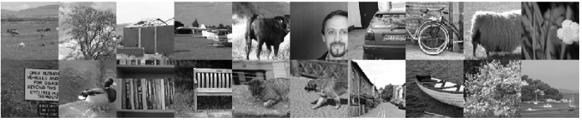
Figure 5: A sample image from each of the 20 types in the Microsoft database. Image statistics were found to vary significantly from one type to another.

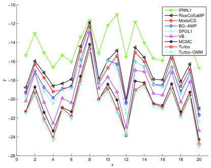
Figure 6: Average NMSE for each image type.

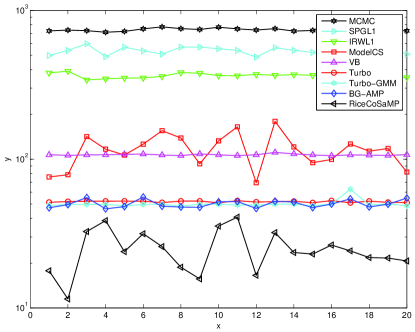
Figure 7: Average runtime for each image type.

Algorithm	NMSE (dB)	Computation Time (sec)
HMT+IRWL1	-14.37	363
CoSaMP	-16.90	25
ModelCS	-17.45	117
BG-AMP	-17.84	68
SPGL1	-18.06	536
VB	-19.04	107
MCMC	-20.10	742
Turbo-BG	-20.49	51
Turbo-GM	-20.74	51

TABLE I: NMSE and runtime averaged over $591$ images.

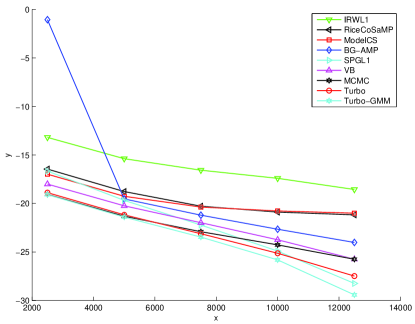
Figure 8: Average NMSE for images of type 1.

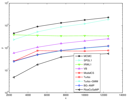
Figure 9: Average runtime for images of type 1.

For a quantitative comparison, we measured average performance over a suite of images in a Microsoft Research Object Class Recognition database that contains $20$ types of images (see Fig. 5) with roughly $30$ images of each type. In particular, we computed the average NMSE and average runtime on a 2.5 GHz PC, for each image type. These results are reported in Figures 6 and 7, and the global averages (over all $591$ images) are reported in Table I. From the table, we observe that the proposed Turbo algorithms outperform all the other tested algorithms in terms of reconstruction NMSE, but are beaten only by CoSaMP in speed. Between the two Turbo algorithms, we observe that Turbo-GM slightly outperforms Turbo-BG in terms of reconstruction NMSE, while taking the same runtime. In terms of NMSE performance, the closest competitor to the Turbo schemes is MCMC, whose NMSE is $0.39$dB worse than Turbo-BG and $0.65$dB worse than Turbo-GM. The good NMSE performance of MCMC comes at the cost of complexity, though: MCMC is $15$ times slower than the Turbo schemes. The second closest NMSE-competitor is VB, showing performance $1.5$ dB worse than Turbo-BG and $1.7$dB worse than Turbo-GM. Even with this sacrifice in performance, VB is still twice as slow as the Turbo schemes. Among the algorithms that do not exploit PAS, we see that SPGL1 offers the best NMSE performance, but is by far the slowest (e.g., $20$ times slower than CoSaMP). Meanwhile, CoSaMP is the fastest, but shows the worst NMSE performance (e.g., $1.16$dB worse than SPGL1). BG-AMP strikes an excellent balance between the two: its NMSE is only $0.22$dB away from SPGL1, whereas it takes only $2.7$ times as long as CoSaMP. However, by combining the AMP algorithm with HMT structure via the turbo approach, it is possible to significantly improve NMSE while simultaneously decreasing the runtime. The reason for the complexity decrease is twofold. First, the HMT structure helps the AMP and parameter-learning iterations to converge faster. Second, the HMT steps are computationally negligible relative to the AMP steps: when, e.g., $M=5000$, the AMP portion of the turbo iteration takes approximately $6$ sec while the HMT portion takes $0.02$ sec.

We also studied NMSE and compute time as a function of the number of measurements, $M$. For this study, we examined images of Type 1 at $M=2500,5000,7500,10000,12500$. In Figure 8, we see that Turbo-GM offers the uniformly best NMSE performance across $M$. However, as $M$ decreases, there is little difference between the NMSEs of Turbo-GM, Turbo-CS, and MCMC. As $M$ increases, though, we see that the NMSEs of MCMC and VB converge, but that they are significantly outperformed by Turbo-GM, Turbo-CS, and—somewhat surprisingly—SPGL1. In fact, at $M=12500$, SPGL1 outperforms Turbo-BG, but not Turbo-GM. However, the excellent performance of SPGL1 at these $M$ comes at the cost of very high complexity, as evident in Figure 9.

V Conclusion

We proposed a new approach to HMT-based compressive imaging based on loopy belief propagation, leveraging a turbo message passing schedule and the AMP algorithm of Donoho, Maleki, and Montanari. We then tested our algorithm on a suite of $591$ natural images and found that it outperformed the state-of-the-art approach (i.e., variational Bayes) while halving its runtime.

References

- [1] J. Romberg, “Imaging via compressive sampling,” IEEE Signal Process. Mag., vol. 25, no. 2, pp. 14–20, Mar. 2008.
- [2] S. Mallat, A Wavelet Tour of Signal Processing, 3rd ed. San Diego, CA: Academic Press, 2008.
- [3] R. G. Baraniuk, V. Cevher, M. F. Duarte, and C. Hegde, “Model-based compressive sensing,” IEEE Trans. Inform. Theory, vol. 56, no. 4, pp. 1982–2001, Apr. 2010.
- [4] M. F. Duarte, M. B. Wakin, and R. G. Baraniuk, “Wavelet-domain compressive signal reconstruction using a hidden Markov tree model,” in Proc. IEEE Int. Conf. Acoust. Speech & Signal Process., Las Vegas, NV, Apr. 2008, pp. 5137–5140.
- [5] L. He and L. Carin, “Exploiting structure in wavelet-based Bayesian compressive sensing,” IEEE Trans. Signal Process., vol. 57, no. 9, pp. 3488–3497, Sep. 2009.
- [6] L. He, H. Chen, and L. Carin, “Tree-structured compressive sensing with variational Bayesian analysis,” IEEE Signal Process. Lett., vol. 17, no. 3, pp. 233–236, Mar. 2010.
- [7] D. Needell and J. A. Tropp, “CoSaMP: Iterative signal recovery from incomplete and inaccurate samples,” Appl. Computational Harmonic Anal., vol. 26, no. 3, pp. 301–321, 2009.
- [8] M. S. Crouse, R. D. Nowak, and R. G. Baraniuk, “Wavelet-based statistical signal processing using hidden Markov models,” IEEE Trans. Signal Process., vol. 46, no. 4, pp. 886–902, Apr. 1998.
- [9] C. P. Robert and G. Casella, Monte Carlo Statistical Methods, 2nd ed. New York: Springer, 2004.
- [10] B. J. Frey and D. J. C. MacKay, “A revolution: Belief propagation in graphs with cycles,” in Adv. in Neural Inform. Processing Syst., M. Jordan, M. S. Kearns, and S. A. Solla, Eds. MIT Press, 1998.
- [11] P. Schniter, “Turbo reconstruction of structured sparse signals,” in Proc. Conf. Inform. Science & Syst., Princeton, NJ, Mar. 2010.
- [12] J. Pearl, Probabilistic Reasoning in Intelligent Systems. San Mateo, CA: Morgan Kaufman, 1988.
- [13] F. R. Kschischang, B. J. Frey, and H.-A. Loeliger, “Factor graphs and the sum-product algorithm,” IEEE Trans. Inform. Theory, vol. 47, pp. 498–519, Feb. 2001.
- [14] D. L. Donoho, A. Maleki, and A. Montanari, “Message passing algorithms for compressed sensing,” Proc. National Academy of Sciences, vol. 106, no. 45, pp. 18 914–18 919, Nov. 2009.
- [15] M. Bayati and A. Montanari, “The dynamics of message passing on dense graphs, with applications to compressed sensing,” IEEE Trans. Inform. Theory, vol. 57, no. 2, pp. 764–785, Feb. 2011.
- [16] A. Gelman, J. B. Carlin, H. S. Stern, and D. B. Rubin, Eds., Bayesian Data Analysis, 2nd ed. CRC Press, 2003.
- [17] G. F. Cooper, “The computational complexity of probabilistic inference using Bayesian belief networks,” Artificial Intelligence, vol. 42, 1990.
- [18] W. T. Freeman, E. C. Pasztor, and O. T. Carmichael, “Learning low-level vision,” Intl. J. Computer Vision, vol. 40, no. 1, pp. 25–47, Oct. 2000.
- [19] R. J. McEliece, D. J. C. MacKay, and J.-F. Cheng, “Turbo decoding as an instance of Pearl’s ‘belief propagation’ algorithm,” IEEE J. Sel. Areas Commun., vol. 16, no. 2, pp. 140–152, Feb. 1998.
- [20] D. J. C. MacKay, Information Theory, Inference, and Learning Algorithms. New York: Cambridge University Press, 2003.
- [21] J. Boutros and G. Caire, “Iterative multiuser joint decoding: Unified framework and asymptotic analysis,” IEEE Trans. Inform. Theory, vol. 48, no. 7, pp. 1772–1793, Jul. 2002.
- [22] D. Baron, S. Sarvotham, and R. G. Baraniuk, “Bayesian compressive sensing via belief propagation,” IEEE Trans. Signal Process., vol. 58, no. 1, pp. 2269–280, Jan. 2010.
- [23] D. L. Donoho, A. Maleki, and A. Montanari, “Message passing algorithms for compressed sensing: I. Motivation and construction,” in Proc. Inform. Theory Workshop, Cairo, Egypt, Jan. 2010.
- [24] S. Som, L. C. Potter, and P. Schniter, “On approximate message passing for reconstruction of non-uniformly sparse signals,” in Proc. National Aerospace and Electronics Conf., Dayton, OH, Jul. 2010.
- [25] E. van den Berg and M. P. Friedlander, “Probing the Pareto frontier for basis pursuit solutions,” SIAM J. Scientific Comput., vol. 31, no. 2, pp. 890–912, 2008.
- [26] J. K. Romberg, H. Choi, and R. G. Baraniuk, “Bayesian tree-structured image modeling using wavelet-domain hidden Markov models,” IEEE Trans. Image Process., vol. 10, no. 7, pp. 1056–1068, Jul. 2001.
- [27] S. Som, L. C. Potter, and P. Schniter, “Compressive Imaging using Approximate Message Passing and a Markov-Tree Prior,” in Proc. Asilomar Conf. Signals Syst. Comput., Pacific Grove, CA, Nov. 2010.