Abstract

We perform the perturbation analysis of the Chern-Simons modified gravity around the AdS₄ spacetimes (its curvature radius $\ell$) to obtain the critical gravity. In general, we could not obtain an explicit form of perturbed Einstein equation which shows a massive graviton propagation clearly, but for the Kerr-Schild perturbation and Chern-Simons coupling $\theta=kx/y$, we find the AdS wave as a single massive solution to the perturbed Einstein equation. Its mass squared is given by $M^{2}=[-9+(2\ell^{2}/k-1)^{2}]/4\ell^{2}$. At the critical point of $M^{2}=0(k=\ell^{2}/2)$, the solution takes the log-form and the linearized excitation energies vanish.

PACS numbers:

Typeset Using LaTeX

1 Introduction

The search for a consistent quantum gravity is mainly being suffered from obtaining a renormalizable and unitary quantum field theory. Stelle has first introduced curvature squared terms of $a(R_{\mu\nu}^{2}-R^{2}/3)+bR^{2}$ in addition to the Einstein-Hilbert term of $R/2\kappa$ [1]. If $ab\not=0$, the renormalizability was achieved, but the unitarity was violated unless $a=0$. This clearly shows that the renormalizability and unitarity exclude to each other. In other words, the renormalizability requires 8 DOF (2 massless graviton, 5 massive graviton from $a$-term, and 1 massive scalar from $b$-term), whereas the unitarity imposes 3 DOF (2 massless graviton and 1 massive scalar). Although the $a$-term of providing massive graviton improves the ultraviolet divergence, it induces ghost excitations which jeopardize the unitarirty. In this sense, a first test for the quantum gravity is to require the unitarity, which means that there are no tachyon and ghost in its particle contents.

To this end, we would like to comment that the critical gravities as candidates for quantum gravity were recently investigated in the AdS spacetimes [2, 3, 4, 5, 6, 7, 8]. At the critical point, a degeneracy takes place and massive gravitons coincide with either massless gravitons ($D>3$) or pure gauge modes ($D=3$). Instead of massive gravitons, an equal amount of logarithmic modes appears in the theory [9]: 1 DOF for topologically massive gravity (TMG) [10], 2 DOF for new massive gravity [11, 12, 13], 5 DOF for higher curvature gravity in 4D [5]. In general, we have $D(D+1)/2-(D+1)$ DOF for massive graviton. However, the non-unitarity issue of the log-gravity is not still resolved [2, 6], indicating that any log-gravity suffers from the ghost problem. Furthermore, the critical gravity on the Schwarzschild-AdS black hole has suffered from the ghost problem when the cross term $E_{\rm cross}$ is non-vanishing [14].

In this work, we introduce a Lorentz-violating theory of Cherns-Simons modified gravity [15]. A silent feature of this theory is the presence of a constant vector $v_{c}$ which spoils the isotropy of spacetime (CPT-symmetry) and is coupled to the Pontryagin density of ${}^{*}RR$. Motivation of considering Cherns-Simons modified gravity is twofold in Minkowski spacetimes: one is its close connection to the TMG which accommodates a single massive graviton in three dimensions [16] and the other is the crucial dependence of massive graviton on a choice of constant vector $v_{c}$. It was shown that a timelike vector of $v_{c}=(\mu,\vec{0})$ did not provide any massive mode, leaving massless graviton with 2 DOF, while a spacelike vector $v_{c}=(0,\vec{v})$ yielded a massive graviton with 5 DOF [17]. However, the authors [18] have shown that the only tachyon- and ghost-free model is the case of timelike vector $v_{c}=(\mu,\vec{0})$, giving 2 DOF. This implies that the role of Chern-Simons term is unclear to show its propagating DOF.

Here we wish to perform the perturbation analysis of the Chern-Simons modified gravity around the AdS₄ spacetimes to obtain the critical gravity, instead of Minkowski spactimes. Under the transverse and traceless gauge, we could not obtain a compactly third-order perturbed equation which shows a massive graviton with 5 DOF, but for the Kerr-Schild perturbation with spacelike vector $v_{c}=k(0,0,1/y,-x/y^{2})$, we find the AdS wave as a single massive graviton propagating on AdS₄ spacetimes. This was found as a solution to the Einstein equation [19]. This (1 DOF) contrasts to propagating DOF of graviton in Minkowski spacetimes. At the critical point of $k=\ell^{2}/2$, the solutions takes the log-form and the linearized excitation energies vanish, which indicates a feature of critical gravity.

2 Chern-Simons modified gravity

Let us first consider the Chern-Simons modified gravity in four dimensions with a cosmological constant ($\Lambda$) whose action is given by

$$S=\frac{1}{16\pi G}\int d^{4}x\sqrt{-g}\Big{\{}R-2\Lambda+\frac{\theta}{4}{}^{*}RR\Big{\}}$$ (2.1)

where $\theta$ is an external function of spacetime and ${}^{*}RR={}^{*}R^{a~{}cd}_{~{}b}R^{b}_{~{}acd}$ is the Pontryagin density with

$${}^{*}R^{a~{}cd}_{~{}b}=\frac{1}{2}\epsilon^{cdef}R^{a}_{~{}bef}.$$ (2.2)

In this expression, $\epsilon^{cdef}$ denotes the four-dimensional Levi-Civita tensor. Varying for $g_{ab}$ on the action (2.1) leads to the Einstein equation which takes the form

$$R_{ab}-\frac{1}{2}g_{ab}R+\Lambda g_{ab}+C_{ab}=0$$ (2.3)

where $C_{ab}$ is the four-dimensional Cotton tensor given by

$$C_{ab}=\nabla_{c}~{}\theta~{}\epsilon^{cde}_{~{}~{}(a}\nabla_{|e|}R_{b)d}+\frac{1}{2}\nabla_{c}\nabla_{d}~{}\theta~{}\epsilon_{(b}^{~{}~{}cef}R^{d}_{~{}~{}a)ef}.$$ (2.4)

Note that $C_{ab}$ is a traceless and symmetric tensor. As a result of applying Bianchi identity to (2.3), one has

$$\nabla^{a}C_{ab}=\Big{[}\frac{\nabla_{b}\theta}{8}\Big{]}~{}{}^{*}R_{acdf}R^{acdf}.$$ (2.5)

On the other hand, one finds that Eq.(2.3) has an AdS₄ solution in which the Riemann tensor, Ricci tensor and Ricci scalar of the AdS₄ spacetimes are given by

$$\bar{R}_{abcd}=\frac{\Lambda}{3}(\bar{g}_{ac}\bar{g}_{bd}-\bar{g}_{ad}\bar{g}_{bc}),~{}~{}~{}\bar{R}_{ab}=\Lambda\bar{g}_{ab},~{}~{}~{}\bar{R}=4\Lambda.$$ (2.6)

Here “overbar” denotes the background AdS₄-metric $\bar{g}_{ab}$.

In order to obtain perturbation equations, we introduce the perturbation around the the background metric as

$$g_{ab}=\bar{g}_{ab}+h_{ab}.$$ (2.7)

The linearized equation to (2.3) can be written by

$$\delta R_{ab}(h)-\frac{1}{2}g_{ab}\delta R(h)-\Lambda h_{ab}+\delta C_{ab}(h)=0,$$ (2.8)

where the linearized tensor $\delta R_{ab}(h),~{}\delta R(h),$ and $\delta C_{ab}(h)$ take the form

$$\delta R_{ab}(h) = \frac{1}{2}\left(\bar{\nabla}^{c}\bar{\nabla}_{a}h_{bc}+\bar{\nabla}^{c}\bar{\nabla}_{b}h_{ac}-\bar{\nabla}^{2}h_{ab}-\bar{\nabla}_{a}\bar{\nabla}_{b}h\right)$$

$$\delta R(h) = \bar{\nabla}^{a}\bar{\nabla}^{b}h_{ab}-\bar{\nabla}^{2}h-\Lambda h$$

$$\delta C_{ab}(h) = \Bigg{[}\frac{1}{2}v_{c}~{}\epsilon^{cde}_{~{}~{}~{}a}\left(\bar{\nabla}_{e}\delta R_{bd}-\Lambda\bar{\nabla}_{e}h_{bd}\right)+\frac{1}{8}v_{cd}~{}\epsilon_{b}^{~{}cef}\Big{(}\bar{\nabla}_{e}\bar{\nabla}_{f}h^{d}_{~{}a}+\bar{\nabla}_{e}\bar{\nabla}_{a}h^{d}_{~{}f}$$ (2.9)

$$-\bar{\nabla}_{e}\bar{\nabla}^{d}h_{af}-\bar{\nabla}_{f}\bar{\nabla}_{e}h^{d}_{~{}a}-\bar{\nabla}_{f}\bar{\nabla}_{a}h^{d}_{~{}e}+\bar{\nabla}_{f}\bar{\nabla}^{d}h_{ae}\Big{)}\Bigg{]}+\Bigg{[}a\leftrightarrow b\Bigg{]}$$

with $v_{c}=\bar{\nabla}_{c}\theta$ and $v_{cd}=\bar{\nabla}_{c}\bar{\nabla}_{d}\theta$. Imposing the transverse and traceless (TT) gauge condition as

$$\bar{\nabla}_{a}h^{ab}=0,~{}~{}h=\bar{g}^{ab}h_{ab}=0$$ (2.10)

which takes into account the diffeomorphism [20]

$$\delta_{\xi}h_{ab}=\bar{\nabla}_{a}\xi_{b}+\bar{\nabla}_{b}\xi_{a},$$ (2.11)

the perturbation equation (2.8) takes a simpler form

$$-\frac{1}{2}\bar{\nabla}^{2}h_{ab}+\frac{\Lambda}{3}h_{ab}+\delta C_{ab}=0.$$ (2.12)

Here the linearized tensor $\delta C_{ab}(h)$ is given by

$$\delta C_{ab}(h) = \Big{[}-\frac{1}{4}v_{c}~{}\epsilon^{cde}_{~{}~{}~{}a}\bar{\nabla}_{e}\bar{\nabla}^{2}h_{bd}+\frac{\Lambda}{6}v_{c}~{}\epsilon^{cde}_{~{}~{}~{}a}\bar{\nabla}_{e}h_{bd}+\frac{1}{4}v_{cd}~{}\epsilon_{b}^{~{}cef}\Big{(}\bar{\nabla}_{e}\bar{\nabla}_{a}h^{d}_{~{}f}-\bar{\nabla}_{e}\bar{\nabla}^{d}h_{af}\Big{)}\Big{]}$$ (2.13)

$$+\Big{[}a\leftrightarrow b\Big{]}.$$

We observe that $\delta C_{ab}(h)$ takes still a complicated form, depending $v_{c}$ and $v_{cd}$.

3 AdS wave as perturbation

It is important to note that the perturbation equation (2.12) has the dependency of $\theta$. For a choice of $\theta=t/\mu$ [15], the Cotton tensor (2.4) reduces to the TMG when choosing the Schwarzschild coordinates. However, in the AdS₄ spacetimes, such a choice is not guaranteed since the second term $v_{ab}$ survives. In the AdS₄ spacetimes, there exists a particular choice of $\theta$ [19] which makes $v_{cd}$ vanish. This choice of $\theta$ could be made by choosing the Poincare coordinates $(u,v,x,y)$ for the AdS₄ spacetimes:

$$\theta=k\frac{x}{y},~{}~{}~{}\bar{g}_{ab}=\phi^{-2}\eta_{ab}=\frac{\ell^{2}}{y^{2}}\eta_{ab},$$ (3.1)

where $k$($>0$) has the dimension of [mass]^-2, $\ell$ is the AdS₄ curvature radius ($\ell^{2}=-3/\Lambda)$ and $\eta_{ab}$ is

$$\eta_{ab}dx^{a}dx^{b}=2dudv+dx^{2}+dy^{2}.$$ (3.2)

Considering Eq.(3.1), Eq.(2.12) becomes

$$\Big{(}\bar{\nabla}^{2}-\frac{2}{3}\Lambda\Big{)}\Big{(}h_{ab}+v_{c}~{}\epsilon^{cde}_{~{}~{}~{}(a}\bar{\nabla}_{|e|}h_{b)d}\Big{)}=0.$$ (3.3)

Alternatively, it leads to

$$\Big{(}\delta_{(a}^{a^{{}^{\prime}}}\delta_{b)}^{d}+\delta_{(a}^{a^{{}^{\prime}}}v_{|c|}~{}\epsilon^{cde}_{~{}~{}~{}b)}\bar{\nabla}_{e}\Big{)}\Big{(}\bar{\nabla}^{2}-\frac{2}{3}\Lambda\Big{)}h_{a^{{}^{\prime}}d}=0$$ (3.4)

which is found by using commutation between two operations in Eq.(3.3). Here, $v_{c}$ is given by

$$v_{c}=k\Bigg{(}0,0,\frac{1}{y},-\frac{x}{y^{2}}\Bigg{)}$$ (3.5)

which may generate the mass. In this case, $v_{c}$ is not a constant vector but a vector field. We wish to comment that Eq.(3.3) is an extended version in four dimensions when comparing with the TMG [21]. In three dimensions, one analyzes the perturbation equation by using $D$-operator

$$\Big{(}D^{\mu/\tilde{\mu}}\Big{)}_{\alpha}^{~{}\beta}=\delta_{\alpha}^{~{}\beta}\pm\frac{1}{\mu}\epsilon_{\alpha}^{~{}\gamma\beta}\bar{\nabla}_{\gamma}.$$ (3.6)

However, it is not easy to apply $D$-operator directly to Eq. (3.3) because $v_{c}$ is not a constant vector. In order to see this case explicitly, we introduce $\hat{D}^{\tilde{M}}$-operator in the AdS₄ spacetimes

$$\Big{(}\hat{D}^{M/\tilde{M}}\Big{)}^{ff^{\prime}}_{ad}=\delta_{(a^{\prime}}^{f}\delta_{d)}^{f^{\prime}}\pm\delta_{(a^{\prime}}^{f}v_{|c|}~{}\epsilon^{cf^{\prime}e}_{~{}~{}~{}~{}d)}\bar{\nabla}_{e}.$$ (3.7)

Then, Eq.(3.4) can be rewritten as

$$\Big{(}\hat{D}^{M}\Big{)}^{a^{\prime}d}_{ab}\Big{(}\bar{\nabla}^{2}-\frac{2}{3}\Lambda\Big{)}h_{a^{\prime}d}=0.$$ (3.8)

Now we use $\hat{D}^{\tilde{M}}\hat{D}^{M}$-operation to find

$$\Big{(}\delta_{(a^{\prime}}^{f}\delta_{d)}^{f^{\prime}}-\delta_{(a^{\prime}}^{f}v_{|c^{\prime}|}~{}\epsilon^{c^{\prime}f^{\prime}e^{\prime}}_{~{}~{}~{}~{}~{}d)}\bar{\nabla}_{e}^{\prime}\Big{)}\Big{(}\delta_{(a}^{a^{\prime}}\delta_{b)}^{d}+\delta_{(a}^{a^{\prime}}v_{|c|}~{}\epsilon^{cde}_{~{}~{}~{}~{}b)}\bar{\nabla}_{e}\Big{)}h_{ff^{\prime}}$$

$$=-4v^{2}\Big{(}\bar{\nabla}^{2}-\frac{2}{3}\Lambda-\frac{1}{v^{2}}\Big{)}h_{ab}+4v^{e^{\prime}}v^{e}\bar{\nabla}_{e^{\prime}}\bar{\nabla}_{e}h_{ab}-2\Lambda\theta v^{e}\bar{\nabla}_{e}h_{ab}-2v^{e}v^{e^{\prime}}\bar{\nabla}^{2}h_{ee^{\prime}}g_{ab}$$

$$+\frac{8}{3}\Lambda v^{e}v^{e^{\prime}}h_{ee^{\prime}}g_{ab}+\Big{[}-2v^{e^{\prime}}v^{e}\bar{\nabla}_{a}\bar{\nabla}_{e}h_{e^{\prime}b}+3v^{e}v_{a}\bar{\nabla}^{2}h_{eb}-\frac{\Lambda}{3}\theta v^{e}\bar{\nabla}_{a}h_{eb}+v^{e^{\prime}}v^{e}\bar{\nabla}_{a}\bar{\nabla}_{b}h_{ee^{\prime}}$$

$$-v^{e}v^{e^{\prime}}\bar{\nabla}_{e^{\prime}}\bar{\nabla}_{a}h_{eb}-\frac{8}{3}\Lambda v^{e}v_{b}h_{ea}+(a\leftrightarrow b)\Big{]}=0$$ (3.9)

with $v^{2}\equiv v_{e}v^{e}$. In obtaining this, we have used the gauge condition (2.10). At this stage, it is very difficult to derive the massive second-order equation,

$$\Big{(}\bar{\nabla}^{2}-\frac{2}{3}\Lambda-M^{2}\Big{)}h_{ab}=0$$ (3.10)

unless we choose a simple form of the metric perturbation $h_{ab}$.

In order to analyze Eq.(3.3), we consider the AdS₄ wave as the Kerr-Schild form

$$h_{ab}=2\varphi\lambda_{a}\lambda_{b},$$ (3.11)

where $\lambda_{a}$ is a null and geodesic vector whose form is given by $\lambda_{a}=(1,0,0,0)$ and $\varphi$ is an arbitrary function of coordinates $(u,v,x,y)$. To maintain the TT gauge condition (2.10), one confines $\varphi$ to $\varphi(u,x,y)$ by requiring the condition of $\lambda_{a}\bar{\nabla}^{a}\varphi=0$ ($\to\partial_{v}\varphi=0$). Plugging $h_{ab}=2\varphi\lambda_{a}\lambda_{b}$ into Eq.(3.3) leads to

$$\lambda_{a^{\prime}}\lambda_{d}\Big{[}\delta_{(a}^{a^{{}^{\prime}}}\delta_{b)}^{d}+\delta_{(a}^{a^{{}^{\prime}}}v_{|c|}~{}\epsilon^{cde}_{~{}~{}~{}b)}\Big{(}\frac{\partial_{e}\phi}{\phi}+\bar{\nabla}_{e}\Big{)}\Big{]}\Big{[}\bar{\nabla}^{2}+\frac{2}{3}\Lambda+\frac{4}{\phi}\partial^{f}\phi~{}\partial_{f}\Big{]}\varphi=0.$$ (3.12)

At this stage, we introduce the separation of variables by considering

$$\varphi(u,x,y)=U(u)X(x)Y(y).$$ (3.13)

Taking into account $\lambda_{a},~{}v_{c},$ and $\phi$, Eq.(3.12) can be reduced to

$$\Big{[}y\partial_{y}+x\partial_{x}+1-\frac{\ell^{2}}{k}\Big{]}\Big{[}y^{2}(\partial_{y}^{2}+\partial_{x}^{2})+2y\partial_{y}-2\Big{]}XY=0.$$ (3.14)

Note that the right bracket in Eq.(3.14) represents the perturbation equation of the massless scalar which corresponds to the right parenthesis of massless tensor in Eq.(3.4). On the other hand, we expect that the left bracket in Eq.(3.14) is related to the massive-mode equation as was suggested in three dimensions [21]. In order to obtain the massive-mode (scalar) equation from the left bracket in Eq.(3.14), we introduce an operator of $y\partial_{y}+A$ with $A$ an arbitrary constant. Furthermore, we assume that $X(x)$=constant. Then, we check that the quadratic perturbation equation yields

$$(y\partial_{y}+A)(y\partial_{y}+1-\ell^{2}/k)Y=0$$

$$\to\Big{[}y^{2}\partial_{y}^{2}+y(2-\ell^{2}/k+A)\partial_{y}+A(1-\ell^{2}/k)\Big{]}Y=0,$$ (3.15)

while the perturbation equation of the massive mode may take the form

$$\Big{[}\bar{\nabla}^{2}+\frac{2}{3}\Lambda+\frac{4}{\phi}\partial^{a}\phi\partial_{a}-M^{2}\Big{]}\varphi=0$$

$$\to\frac{1}{\ell^{2}}\Big{[}y^{2}\partial_{y}^{2}+2y\partial_{y}-2-M^{2}\ell^{2}\Big{]}Y=0.$$ (3.16)

Comparing Eq.(3.15) with Eq.(3.16), we find

$$A=\frac{\ell^{2}}{k},~{}~{}\frac{\ell^{2}}{k}=\frac{1}{2}\Big{(}1+\sqrt{9+4\ell^{2}M^{2}}\Big{)}.$$ (3.17)

It is worth noting that for real $\ell^{2}/k$, the allowed region of $M^{2}$ is given by

$$M^{2}=\frac{1}{4\ell^{2}}\Big{[}-9+\left(\frac{2\ell^{2}}{k}-1\right)^{2}\Big{]}\geq M^{2}_{\rm BF}=-\frac{9}{4\ell^{2}},$$ (3.18)

where $M^{2}_{\rm BF}$ corresponds to the Breitenlohner-Freedman (BF) bound for a massive scalar in AdS₄ spacetimes [23]. This occurs also for $k=2\ell^{2}$. Importantly, in the critical limit of $M^{2}\to 0$, we obtain $k=\ell^{2}/2$ from Eq.(3.17). In addition, we note that for $k>\ell^{2}/2$, we have an allowed bound for negative $M^{2}$ (see Fig.1)

$$M^{2}_{\rm BF}\leq M^{2}<0$$ (3.19)

which was also derived from the tensor analysis in the higher curvature gravity including the conformal gravity [22].

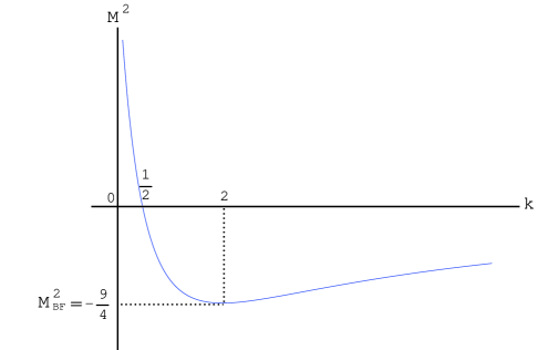
Figure 1: $M^{2}$ graph as function of $k$ with $\ell^{2}=1$. For $k>1/2$ ($M^{2}<0$), the AdS wave is a stable solution because it satisfies the BF bound, $M^{2}\geq M_{BF}^{2}=-9/4$. Hence we have the stable region for positive $k$ ($k>0$). The figure shows that the critical point is located at $k=1/2$ which corresponds to $M^{2}=0$. Also, in the limit of $k\to\infty$, it approaches $M^{2}=-2$.

Consequently, Eq.(3.14) reduces to the third-order equation for $y$

$$\Bigg{[}y\partial_{y}+\frac{1}{2}\Bigg{(}1-2\ell\sqrt{M^{2}+\frac{9}{4\ell^{2}}}~{}\Bigg{)}\Bigg{]}\Big{[}y\partial_{y}-1\Big{]}\Big{[}y\partial_{y}+2\Big{]}Y=0.$$ (3.20)

Now we solve Eq.(3.20) for two cases:

(i) $k\neq\ell^{2}/2$ $(M^{2}\neq 0)$

$$\varphi(u,y)=U(u)Y(y)=c_{1}(u)y^{\frac{1}{2}[-1+2\ell\sqrt{M^{2}+9/4\ell^{2}}]}+c_{2}(u)\frac{1}{y^{2}}+c_{3}(u)y,$$ (3.21)

which is a single massive solution in AdS₄ spacetimes.

(ii) $k=\ell^{2}/2$ ($M^{2}=0$)
In this case, Eq.(3.20) degenerates as

$$(y\partial_{y}+2)(y\partial_{y}-1)^{2}Y=0.$$ (3.22)

We obtain the solution as

$$\varphi(u,y)=U(u)Y(y)=c_{4}(u)y\ln(y)+c_{5}(u)\frac{1}{y^{2}}+c_{6}(u)y.$$ (3.23)

In this approach, $c_{i}(u)$ as functions of $u$ remain undetermined.

We note that the solution (3.23) will be a half of the solution obtained from higher curvature gravity which gives the fourth-order perturbation equation at the critical point [24]. To see this more closely, we construct the fourth-order equation instead of the third-order equation (3.20) by considering

$$\Big{[}(y\partial_{y}+\ell^{2}/k)(y\partial_{y}+1-\ell^{2}/k)\Big{]}\Big{[}(y\partial_{y}-1)(y\partial_{y}+2)\Big{]}Y=0.$$ (3.24)

For $k\neq\ell^{2}/2$, the solution to Eq.(3.24) is given by $Y=Y_{1}+Y_{2}$ where $Y_{1}$ and $Y_{2}$ satisfy the following second-order equations, respectively:

$$\Big{[}(y\partial_{y}+\ell^{2}/k)(y\partial_{y}+1-\ell^{2}/k)\Big{]}Y_{1}=0,~{}~{}~{}\Big{[}(y\partial_{y}-1)(y\partial_{y}+2)\Big{]}Y_{2}=0.$$ (3.25)

The corresponding solutions and combined solution are

$$Y_{1}(y)=d_{1}y^{\frac{1}{2}[-1+2\ell\sqrt{M^{2}+9/4\ell^{2}}]}+d_{2}y^{-\frac{1}{2}[1+2\ell\sqrt{M^{2}+9/4\ell^{2}}]},$$ (3.26)

$$Y_{2}(y)=d_{3}y^{-2}+d_{4}y,$$ (3.27)

$$\rightarrow Y(=Y_{1}+Y_{2})=d_{1}y^{\frac{1}{2}[-1+2\ell\sqrt{M^{2}+9/4\ell^{2}}]}+d_{2}y^{-\frac{1}{2}[1+2\ell\sqrt{M^{2}+9/4\ell^{2}}]}+d_{3}y^{-2}+d_{4}y,$$ (3.28)

where $M^{2}$ appeared in (3.18) and $d_{i}$ are undetermined constants. We note that although the solution form is the same as found in the higher curvature gravity [24], the mass squared $M^{2}$ in (3.18) is different from that [(8) in [24]] in the higher curvature gravity. At the critical point of $M^{2}=0$ ($k=\ell^{2}/2$), the fourth-order equation reduces to

$$\Big{[}\Big{(}y\partial_{y}-1\Big{)}\Big{(}y\partial_{y}+2\Big{)}\Big{]}^{2}Y=0,$$ (3.29)

whose solution is given by

$$Y(y)=d_{5}y\ln(y)+d_{6}\frac{1}{y^{2}}+d_{7}y+\frac{d_{8}}{y^{2}}\ln(y)$$ (3.30)

which shows that the last term is absent in (3.23). This solution is exactly the same found in the higher curvature gravity [24].

4 Linear excitation energy

In the perturbation analysis, it is important to check whether the ghost mode exists or not. For this purpose, we construct the Hamiltonian of the action. Firstly, the quadratic action of $h_{ab}$ takes the form

$$S^{(2)} = -\frac{1}{16\pi G}\int d^{4}x\sqrt{-g}h^{ab}\Big{[}\delta\Big{(}R_{ab}-\frac{1}{2}g_{ab}R+\Lambda g_{ab}\Big{)}+\delta C_{ab}\Big{]}$$ (4.1)

$$= -\frac{1}{16\pi G}\int d^{4}x\sqrt{-g}\Big{[}\frac{1}{2}(\bar{\nabla}^{c}h^{ab})(\bar{\nabla}_{c}h_{ab})+\frac{\Lambda}{3}h^{ab}h_{ab}+\frac{1}{2}\epsilon^{cde}_{~{}~{}~{}a}\Big{(}v_{ce}h^{ab}\bar{\nabla}^{2}h_{bd}$$

$$+v_{c}\bar{\nabla}_{e}h^{ab}\bar{\nabla}^{2}h_{bd}+\frac{2}{3}\Lambda v_{c}h^{ab}\bar{\nabla}_{e}h_{bd}\Big{)}-\frac{1}{2}\epsilon_{b}^{~{}cef}\Big{(}v_{cde}h^{ab}\bar{\nabla}_{a}h^{d}_{~{}f}+v_{cd}\bar{\nabla}_{e}h^{ab}\bar{\nabla}_{a}h^{d}_{~{}f}$$

$$-v_{cde}h^{ab}\bar{\nabla}^{d}h_{af}-v_{cd}\bar{\nabla}_{e}h^{ab}\bar{\nabla}^{d}h_{af}\Big{)}\Big{]}.$$

From the action (4.1), we define the conjugate momentum given by

$$\Pi^{ab}_{(1)}=-\bar{\nabla}^{2}h^{ab}-\frac{1}{2}\epsilon^{cd0a}v_{c}\bar{\nabla}^{2}h^{b}_{~{}d}-\frac{\Lambda}{3}v_{c}\epsilon^{ca0}_{~{}~{}~{}d}h^{db}+\frac{1}{2}\epsilon^{bc0f}v_{cd}\bar{\nabla}^{a}h^{d}_{~{}f}+\frac{1}{2}\epsilon_{f}^{~{}ceb}v_{c}^{a}\bar{\nabla}_{e}h^{0f}$$

$$\hskip 10.00002pt-\frac{1}{2}\epsilon_{f}^{~{}ceb}v_{c~{}e}^{~{}0}h^{af}-\frac{1}{2}\epsilon^{bc0f}v_{cd}\bar{\nabla}^{d}h^{a}_{~{}f}-\frac{1}{2}\epsilon_{f}^{~{}ceb}v_{c}^{0}\bar{\nabla}_{e}h^{af}+\frac{1}{2}\bar{\nabla}^{0}(\epsilon^{cae}_{~{}~{}~{}d}v_{c}\bar{\nabla}_{e}h^{db}\bar{g}^{00}).$$ (4.2)

Using the method of Ostrogradsky, we find the conjugate momentum for the second-time derivative as

$$\Pi^{ab}_{(2)}=-\frac{1}{2}\bar{\nabla}^{0}(\epsilon^{cae}_{~{}~{}~{}d}v_{c}\bar{\nabla}_{e}h^{db}\bar{g}^{00}).$$ (4.3)

Then the Hamiltonian can be written by

$$H=\int d^{4}x\Big{(}\dot{h}_{ab}\Pi^{ab}_{(1)}+\dot{K}_{ai}\Pi^{ai}_{(2)}\Big{)}-S^{(2)}$$ (4.4)

with $K_{ai}=\bar{\nabla}_{0}h_{ai}$. Considering (3.1) and (3.11), one finds that the Hamiltonian (4.4) is identically zero ($H=0$), irrespective of any solution form $\varphi$. This means that there is no ghost for AdS waves.

5 Discussions

In the Minkowski spacetimes, the ghost- and tachyon-free mode of Chern-Simons modified gravity is just a massless graviton with 2 DOF [18]. This amounts to the choice of a timelike vector $v_{c}=(\mu,\vec{0})$.

In general, it is a formidable task to find a massive graviton with 5 DOF in the AdS₄ spacetimes because its linearized equation is a very complicated form, compared to the TMG, showing a single massive scalar [21]. However, choosing $v_{c}$ as a vector field (3.5) which makes the perturbation equation simple and then, the Kerr-Schild perturbation (3.11), we have a single massive scalar $\varphi$ propagating on the AdS₄ spacetimes. This is ghost-free and tachyon-free if the mass squared (3.18) satisfies the BF bound $M^{2}\geq M^{2}_{\rm BF}$. Even for the negative bound of $-M^{2}_{\rm BF}\leq M^{2}<0$, there is no tachyon instability (no exponentially growing modes) [22]. At the critical point of $M^{2}=0(k=\ell^{2}/2$), we have found the log-form without ghost, which is the half solution found in the higher curvature gravity [24].

However, it seems difficult to derive a massive graviton with 5 DOF propagating in the AdS₄ spacetimes from the Chern-Simons modified gravity, compared to the higher curvature gravity [9]. This is mainly because massive excitations depend critically on the choice of coupling field $v_{c}(\theta)$.

Acknowledgments

This work was supported by the National Research Foundation of Korea (NRF) grant funded by the Korea government (MEST) through the Center for Quantum Spacetime (CQUeST) of Sogang University with grant number 2005-0049409. Y. Myung was partly supported by the National Research Foundation of Korea (NRF) grant funded by the Korea government (MEST) (No.2011-0027293).

References

- [1] K. S. Stelle, Phys. Rev. D 16, 953 (1977).
- [2] H. Lu and C. N. Pope, Phys. Rev. Lett. 106, 181302 (2011) [arXiv:1101.1971 [hep-th]].
- [3] S. Deser, H. Liu, H. Lu, C. N. Pope, T. C. Sisman and B. Tekin, Phys. Rev. D 83, 061502 (2011) [arXiv:1101.4009 [hep-th]].
- [4] M. Alishahiha and R. Fareghbal, Phys. Rev. D 83, 084052 (2011) [arXiv:1101.5891 [hep-th]].
- [5] E. A. Bergshoeff, O. Hohm, J. Rosseel and P. K. Townsend, Phys. Rev. D 83, 104038 (2011) [arXiv:1102.4091 [hep-th]].
- [6] M. Porrati and M. M. Roberts, Phys. Rev. D 84, 024013 (2011) [arXiv:1104.0674 [hep-th]].
- [7] Y. S. Myung, Y. W. Kim and Y. J. Park, arXiv:1106.0546 [hep-th].
- [8] Y. S. Myung, arXiv:1107.3594 [hep-th].
- [9] E. A. Bergshoeff, S. de Haan, W. Merbis and J. Rosseel, arXiv:1106.6277 [hep-th].
- [10] D. Grumiller and N. Johansson, JHEP 0807, 134 (2008) [arXiv:0805.2610 [hep-th]].
- [11] Y. Liu and Y. W. Sun, JHEP 0905, 039 (2009) [arXiv:0903.2933 [hep-th]].
- [12] D. Grumiller and O. Hohm, Phys. Lett. B 686, 264 (2010) [arXiv:0911.4274 [hep-th]].
- [13] Y. S. Myung, Y. W. Kim, T. Moon and Y. J. Park, Phys. Rev. D 84, 024044 (2011) [arXiv:1105.4205 [hep-th]].
- [14] H. Liu, H. Lu and M. Luo, arXiv:1104.2623 [hep-th].
- [15] R. Jackiw and S.Y. Pi, Phys. Rev. D68, 104012 (2003) [gr-qc/0308071].
- [16] S. Deser, R. Jackiw and S. Templeton, Annals Phys. 140, 372 (1982) [Erratum-ibid. 185, 406 (1988)] [Annals Phys. 185, 406 (1988)] [Annals Phys. 281, 409 (2000)].
- [17] J. L. Boldo, J. A. Helayel-Neto, L. M. de Moraes, C. A. G. Sasaki and V. J. Vasquez Otoya, Phys. Lett. B 689, 112 (2010) [arXiv:0903.5207 [hep-th]].
- [18] B. Pereira-Dias, C. A. Hernaski and J. A. Helayel-Neto, Phys. Rev. D 83, 084011 (2011) [arXiv:1009.5132 [hep-th]].
- [19] E. A.-Beato, G. Giribet, and M. Hassaine, Phys. Rev. D83, 104033 (2011) [arXiv:1103.0742 [hep-th]].
- [20] B. Tekin, Phys. Rev. D 77, 024005 (2008) [arXiv:0710.2528 [gr-qc]].
- [21] W. Li, W. Song and A. Strominger, JHEP 0804, 082 (2008) [arXiv:0801.4566 [hep-th]].
- [22] H. Lu, Y. Pang and C. N. Pope, arXiv:1106.4657 [hep-th].
- [23] P. Breitenlohner and D. Z. Freedman, Annals Phys. 144, 249 (1982).
- [24] I. Gullu, M. Gurses, T. C. Sisman, and B. Tekin, Phys. Rev. D83, 084015 (2011) [arXiv:1102.1921 [hep-th]].