Calculation of all elements of the Mueller matrix for scattering of light from a two-dimensional randomly rough metal surface

P. A. Letnes Paul.Anton.Letnes@gmail.com Department of Physics, Norwegian University of Science and Technology, NO-7491 Trondheim, Norway    A. A. Maradudin aamaradu@uci.edu Department of Physics and Astronomy, and Institute for Surface and Interface Science, University of California, Irvine, CA 92697 USA    T. Nordam Tor.Nordam@ntnu.no Department of Physics, Norwegian University of Science and Technology, NO-7491 Trondheim, Norway    I. Simonsen Ingve.Simonsen@ntnu.no Department of Physics, Norwegian University of Science and Technology, NO-7491 Trondheim, Norway
Abstract

We calculate all the elements of the Mueller matrix, which contains all the polarization properties of light scattered from a two-dimensional randomly rough lossy metal surface. The calculations are carried out for arbitrary angles of incidence by the use of nonperturbative numerical solutions of the reduced Rayleigh equations for the scattering of p- and s-polarized light from a two-dimensional rough penetrable surface. The ability to model polarization effects in light scattering from surfaces enables better interpretation of experimental data and allows for the design of surfaces which possess useful polarization effects.

pacs:
42.25.-p, 41.20.-q

When light undergoes scattering from a surface, the scattered light carries a great deal of information about the statistical properties of the surface in its polarization. Even when the structures in question are sub-wavelength and beyond the imaging limit, polarized optical scattering can be employed to detect and distinguish between material inhomogeneities, particles, or even buried defects and the roughness of both interfaces of thin films Germer (2007). These techniques are already in use in the semiconductor industry, and such techniques could become important for surface characterization of photovoltaic materials and nanomaterials Drezet et al. (2008); Kullock et al. (2008). Many biological materials are optically active, meaning that polarimetric measurements may be applied for characterization of biological or hybrid Schmidt et al. (2011) materials and even for the search for extra-terrestrial life Martin et al. (2010). Surface patterning has also been proven as a method for creating optical components with interesting polarization properties Ghadyani et al. (2011).

To extract this information from experimental data, one has to be able to model polarization effects Ellis et al. (2002). The ability to calculate the polarization of the scattered light also opens the door to the possibility of designing surfaces that produce specified polarization properties of the light scattered from them.

All the information about the polarization properties of light scattered from two-dimensional surfaces is contained in the Mueller matrix Mueller (1948); Bickel and Bailey (1985); Chipman (1994). Yet, very few calculations of the elements of this matrix for a two-dimensional randomly rough surface have to date been carried out by any computational approach, largely because calculations of the scattering of light from such surfaces are still difficult to carry out Simonsen et al. (2010a, b); Nordam et al. ; Simonsen et al. (2011). An exception Bruce (1998) is a calculation of the Mueller matrix for two-dimensional randomly rough perfectly conducting and metallic surfaces characterized by a surface profile function that is a stationary, zero-mean, isotropic, Gaussian random process, defined by a Gaussian surface height autocorrelation function. These calculations were carried out by a ray-tracing approach on the assumption that the surface was illuminated at normal incidence. In this work it was also shown that due to the assumptions of normal incidence and the isotropy of the surface statistics, the elements of the corresponding Mueller matrix possess certain symmetry properties. Subsequently Zhang and Bahar Zhang and Bahar (1999) carried out an approximate analytic calculation of the elements of the Mueller matrix for the scattering of light from two-dimensional randomly rough dielectric surfaces coated uniformly with a different dielectric material.

In this Letter we report the first step toward realizing the possibilities mentioned in the opening paragraphs. We present an approach to calculating, for arbitrary angles of incidence, all the elements of the Mueller matrix for the scattering of light from a two-dimensional randomly rough metal surface. It is based on nonperturbative numerical solutions of the reduced Rayleigh equations for the scattering of p- and s-polarized light from a two-dimensional rough penetrable surface Nordam et al. ; Brown et al. (1984).

The system we study consists of vacuum in the region $x_{3}>\zeta(\mathbf{{x}}_{\parallel})$, where $\mathbf{{x}}_{\parallel}=(x_{1},x_{2},0)$, and a metal whose dielectric function is $\varepsilon(\omega)$ in the region $x_{3}<\zeta(\mathbf{{x}}_{\parallel})$. The surface profile function $\zeta(\mathbf{{x}}_{\parallel})$ is assumed to be a single-valued function of $\mathbf{{x}}_{\parallel}$ that is differentiable with respect to $x_{1}$ and $x_{2}$, and constitutes a stationary, zero-mean, isotropic, Gaussian random process defined by $\left<\zeta(\mathbf{{x}}_{\parallel})\zeta(\mathbf{{x}}_{\parallel}^{\prime})\right>=\delta^{2}W\left(\left|\mathbf{{x}}_{\parallel}-\mathbf{{x}}_{\parallel}^{\prime}\right|\right)$. The angle brackets here and in all that follows denote an average over the ensemble of realizations of the surface profile function, and $\delta=\left<\zeta^{2}(\mathbf{{x}}_{\parallel})\right>^{1/2}$ is the rms height of the surface. Each realization of the surface profile function was generated numerically by the filtering method used in Refs. Simonsen et al. (2011); Maradudin et al. (1990).

We begin by writing the electric field in the vacuum region $x_{3}>\zeta(\mathbf{{x}}_{\parallel})$ as the sum of an incident and a scattered field, $\mathbf{{E}}(\mathbf{{x}},t)=\left[\mathbf{{E}}^{(i)}(\mathbf{{x}}|\omega)+\mathbf{{E}}^{(s)}(\mathbf{{x}}|\omega)\right]\exp(-\mathrm{i}\omega t)$, where

$\displaystyle\mathbf{{E}}^{(i)}(\mathbf{{x}}|\omega)$ $\displaystyle=\left[{\mathcal{E}}^{(i)}_{p}(\mathbf{{k}}_{\parallel})\mathbf{{\hat{e}}}^{(i)}_{p}(\mathbf{{k}}_{\parallel})+{\mathcal{E}}^{(i)}_{s}(\mathbf{{k}}_{\parallel})\mathbf{{\hat{e}}}^{(i)}_{s}(\mathbf{{k}}_{\parallel})\right]\exp\left[\mathrm{i}\mathbf{{k}}_{\parallel}\cdot\mathbf{{x}}_{\parallel}-\mathrm{i}\alpha_{0}(k_{\parallel})x_{3}\right],$
$\displaystyle\mathbf{{E}}^{(s)}(\mathbf{{x}}|\omega)$ $\displaystyle=\int\!\!\frac{\mathrm{d}^{2}q_{\parallel}}{(2\pi)^{2}}\>\left[{\mathcal{E}}^{(s)}_{p}(\mathbf{{q}}_{\parallel})\mathbf{{\hat{e}}}^{(s)}_{p}(\mathbf{{q}}_{\parallel})+{\mathcal{E}}^{(s)}_{s}(\mathbf{{q}}_{\parallel})\mathbf{{\hat{e}}}^{(s)}_{s}(\mathbf{{q}}_{\parallel})\right]\exp[\mathrm{i}\mathbf{{q}}_{\parallel}\cdot\mathbf{{x}}_{\parallel}+\mathrm{i}\alpha_{0}(q_{\parallel})x_{3}].$

Here $\mathbf{{k}}_{\parallel}=(k_{1},k_{2},0)$, the unit polarization vectors are $\mathbf{{\hat{e}}}^{(i)}_{p}(\mathbf{{k}}_{\parallel})=(c/\omega)\left[\alpha_{0}(k_{\parallel})\mathbf{{\hat{k}}}_{\parallel}+k_{\parallel}\mathbf{{\hat{x}}}_{3}\right]$, $\mathbf{{\hat{e}}}^{(i)}_{s}(\mathbf{{k}}_{\parallel})=\mathbf{{\hat{k}}}_{\parallel}\times\mathbf{{\hat{x}}}_{3}$, $\mathbf{{\hat{e}}}^{(s)}_{p}(\mathbf{{q}}_{\parallel})=(c/\omega)\left[-\alpha_{0}(q_{\parallel})\mathbf{{\hat{q}}}_{\parallel}+q_{\parallel}\mathbf{{\hat{x}}}_{3}\right]$, $\mathbf{{\hat{e}}}^{(s)}_{s}(\mathbf{{q}}_{\parallel})=\mathbf{{\hat{q}}}_{\parallel}\times\mathbf{{\hat{x}}}_{3}$, while $\alpha_{0}(q_{\parallel})=\left[(\omega/c)^{2}-q_{\parallel}^{2}\right]^{1/2}$, with $\mathrm{Re}\,\alpha_{0}(q_{\parallel})>0$, $\mathrm{Im}\,\alpha_{0}(q_{\parallel})>0$. A caret over a vector indicates that it is a unit vector. In terms of the polar and azimuthal angles of incidence $(\theta_{0},\phi_{0})$ and scattering $(\theta_{s},\phi_{s})$, the vectors $\mathbf{{k}}_{\parallel}$ and $\mathbf{{q}}_{\parallel}$ are given by $\mathbf{{k}}_{\parallel}=(\omega/c)\sin\theta_{0}(\cos\phi_{0},\sin\phi_{0},0)$ and $\mathbf{{q}}_{\parallel}=(\omega/c)\sin\theta_{s}(\cos\phi_{s},\sin\phi_{s},0)$.

A linear relation exists between the amplitudes ${\mathcal{E}}^{(s)}_{\alpha}(\mathbf{{q}}_{\parallel})$ and ${\mathcal{E}}^{(i)}_{\beta}(\mathbf{{k}}_{\parallel})$, which we write in the form $(\alpha=p,s$, $\beta=p,s)$

$\displaystyle{\mathcal{E}}^{(s)}_{\alpha}(\mathbf{{q}}_{\parallel})$ $\displaystyle=\sum_{\beta}R_{\alpha\beta}(\mathbf{{q}}_{\parallel}|\mathbf{{k}}_{\parallel}){\mathcal{E}}^{(i)}_{\beta}(\mathbf{{k}}_{\parallel}).$

It was shown by Celli and his colleagues Brown et al. (1984) that the scattering amplitudes $R_{\alpha\beta}(\mathbf{{q}}_{\parallel}|\mathbf{{k}}_{\parallel})$ satisfy the matrix integral equation (the reduced Rayleigh equation)

$\displaystyle\int$ $\displaystyle\frac{\mathrm{d}^{2}q_{\parallel}}{(2\pi)^{2}}\;\frac{I\left(\alpha(p_{\parallel})-\alpha_{0}(q_{\parallel})|\mathbf{{p}}_{\parallel}-\mathbf{{q}}_{\parallel}\right)}{\alpha(p_{\parallel})-\alpha_{0}(q_{\parallel})}\mbox{\boldmath${\mathcal{N}}$}_{+}(\mathbf{{p}}_{\parallel}|\mathbf{{q}}_{\parallel})\mathbf{{R}}(\mathbf{{q}}_{\parallel}|\mathbf{{k}}_{\parallel})$
$\displaystyle\quad=-\frac{I\left(\alpha(p_{\parallel})+\alpha_{0}(k_{\parallel})|\mathbf{{p}}_{\parallel}-\mathbf{{k}}_{\parallel}\right)}{\alpha(p_{\parallel})+\alpha_{0}(k_{\parallel})}\mbox{\boldmath${\mathcal{N}}$}_{-}(\mathbf{{p}}_{\parallel}|\mathbf{{k}}_{\parallel}),$ (2)

with $R_{pp}$ and $R_{ps}$ forming the first row of the matrix $\mathbf{{R}}$, where

$\displaystyle I\left(\gamma|\mathbf{{Q}}_{\parallel}\right)=\int\mathrm{d}^{2}x_{\parallel}\;\exp[-\mathrm{i}\gamma\zeta(\mathbf{{x}}_{\parallel})]\exp(-\mathrm{i}\mathbf{{Q}}_{\parallel}\cdot\mathbf{{x}}_{\parallel}),$ (3)

and $\alpha(p_{\parallel})=\left[\varepsilon(\omega)(\omega/c)^{2}-p_{\parallel}^{2}\right]^{1/2}$, with $\mathrm{Re}\,\alpha(p_{\parallel})>0$, $\mathrm{Im}\,\alpha(p_{\parallel})>0$. The matrices $\mbox{\boldmath${\mathcal{N}}$}_{\pm}\left(\mathbf{{p}}_{\parallel}|\mathbf{{q}}_{\parallel}\right)$ are given by

$\displaystyle\mbox{\boldmath${\mathcal{N}}$}_{\pm}$ $\displaystyle(\mathbf{{p}}_{\parallel}|\mathbf{{q}}_{\parallel})=$
$\displaystyle\begin{pmatrix}p_{\parallel}q_{\parallel}\pm\alpha(p_{\parallel})\mathbf{{\hat{p}}}_{\parallel}\cdot\mathbf{{\hat{q}}}_{\parallel}\alpha_{0}(q_{\parallel})&-\frac{\omega}{c}\alpha(p_{\parallel})(\mathbf{{\hat{p}}}_{\parallel}\times\mathbf{{\hat{q}}}_{\parallel})_{3}\\ \pm\frac{\omega}{c}(\mathbf{{\hat{p}}}_{\parallel}\times\mathbf{{\hat{q}}}_{\parallel})_{3}\alpha_{0}(q_{\parallel})&\frac{\omega^{2}}{c^{2}}\mathbf{{\hat{p}}}_{\parallel}\cdot\mathbf{{\hat{q}}}_{\parallel}\end{pmatrix}.$

These equations were solved by the method described in detail in Nordam et al. . First, a realization of the surface profile function on a grid of $N^{2}_{x}$ points within a square region of the $x_{1}x_{2}$ plane of edge $L$. In evaluating the $\mathbf{{q}}_{\parallel}$-integral in Eq. (2) the infinite limits of integration were replaced by finite ones: $\left|\mathbf{{q}}_{\parallel}\right|<Q/2$, and the integral was carried out by a two-dimensional version of the extended midpoint rule Press et al. (1992) using a grid in the $q_{1}q_{2}$ plane that is determined by the Nyquist sampling theorem and the properties of the discrete Fourier transform. The function $I(\gamma|\mathbf{{Q}}_{\parallel})$ was evaluated by expanding the integrand in Eq. (3) in powers of $\zeta(\mathbf{{x}}_{\parallel})$ and calculating the Fourier transform of $\zeta^{n}(\mathbf{{x}}_{\parallel})$ by the Fast Fourier Transform. The resulting equations were solved by LU factorization.

The scattering amplitudes $R_{\alpha\beta}(\mathbf{{q}}_{\parallel}|\mathbf{{k}}_{\parallel})$ play a central role in the calculation of the elements of the Mueller matrix. In terms of these amplitudes the elements of the Mueller matrix, $\mathbf{{M}}$, are 111A. A. Maradudin (unpublished)

$\displaystyle M_{11}$ $\displaystyle=C\left(|R_{\mathrm{pp}}|^{2}+|R_{\mathrm{sp}}|^{2}+|R_{\mathrm{ps}}|^{2}+|R_{\mathrm{ss}}|^{2}\right)$
$\displaystyle M_{12}$ $\displaystyle=C\left(|R_{\mathrm{pp}}|^{2}+|R_{\mathrm{sp}}|^{2}-|R_{\mathrm{ps}}|^{2}-|R_{\mathrm{ss}}|^{2}\right)$
$\displaystyle M_{13}$ $\displaystyle=C\left(R_{\mathrm{pp}}R_{\mathrm{ps}}^{*}+R_{\mathrm{sp}}R_{\mathrm{ss}}^{*}+R_{\mathrm{ps}}R_{\mathrm{pp}}^{*}+R_{\mathrm{ss}}R_{\mathrm{sp}}^{*}\right)$
$\displaystyle M_{14}$ $\displaystyle=\mathrm{i}C\left(R_{\mathrm{pp}}R^{*}_{\mathrm{ps}}+R_{\mathrm{sp}}R^{*}_{\mathrm{ss}}-R_{\mathrm{ps}}R^{*}_{\mathrm{pp}}-R_{\mathrm{ss}}R^{*}_{\mathrm{sp}}\right)$
$\displaystyle M_{21}$ $\displaystyle=C\left(|R_{\mathrm{pp}}|^{2}-|R_{\mathrm{sp}}|^{2}+|R_{\mathrm{ps}}|^{2}-|R_{\mathrm{ss}}|^{2}\right)$
$\displaystyle M_{22}$ $\displaystyle=C\left(|R_{\mathrm{pp}}|^{2}-|R_{\mathrm{sp}}|^{2}-|R_{\mathrm{ps}}|^{2}+|R_{\mathrm{ss}}|^{2}\right)$
$\displaystyle M_{23}$ $\displaystyle=C\left(R_{\mathrm{pp}}R^{*}_{\mathrm{ps}}-R_{\mathrm{sp}}R^{*}_{\mathrm{ss}}+R_{\mathrm{ps}}R^{*}_{\mathrm{pp}}-R_{\mathrm{ss}}R^{*}_{\mathrm{sp}}\right)$
$\displaystyle M_{24}$ $\displaystyle=\mathrm{i}C\left(R_{\mathrm{pp}}R^{*}_{\mathrm{ps}}-R_{\mathrm{sp}}R^{*}_{\mathrm{ss}}-R_{\mathrm{ps}}R^{*}_{\mathrm{pp}}+R_{\mathrm{ss}}R^{*}_{\mathrm{sp}}\right)$
$\displaystyle M_{31}$ $\displaystyle=C\left(R_{\mathrm{pp}}R^{*}_{\mathrm{sp}}+R_{\mathrm{sp}}R^{*}_{\mathrm{pp}}+R_{\mathrm{ps}}R^{*}_{\mathrm{ss}}+R_{\mathrm{ss}}R^{*}_{\mathrm{ps}}\right)$
$\displaystyle M_{32}$ $\displaystyle=C\left(R_{\mathrm{pp}}R^{*}_{\mathrm{sp}}+R_{\mathrm{sp}}R^{*}_{\mathrm{pp}}-R_{\mathrm{ps}}R^{*}_{\mathrm{ss}}-R_{\mathrm{ss}}R^{*}_{\mathrm{ps}}\right)$
$\displaystyle M_{33}$ $\displaystyle=C\left(R_{\mathrm{pp}}R^{*}_{\mathrm{ss}}+R_{\mathrm{sp}}R^{*}_{\mathrm{ps}}+R_{\mathrm{ps}}R^{*}_{\mathrm{sp}}+R_{\mathrm{ss}}R^{*}_{\mathrm{pp}}\right)$
$\displaystyle M_{34}$ $\displaystyle=\mathrm{i}C\left(R_{\mathrm{pp}}R^{*}_{\mathrm{ss}}+R_{\mathrm{sp}}R^{*}_{\mathrm{ps}}-R_{\mathrm{ps}}R^{*}_{\mathrm{sp}}-R_{\mathrm{ss}}R^{*}_{\mathrm{pp}}\right)$
$\displaystyle M_{41}$ $\displaystyle=-\mathrm{i}C\left(R_{\mathrm{pp}}R^{*}_{\mathrm{sp}}-R_{\mathrm{sp}}R^{*}_{\mathrm{pp}}+R_{\mathrm{ps}}R^{*}_{\mathrm{ss}}-R_{\mathrm{ss}}R^{*}_{\mathrm{ps}}\right)$
$\displaystyle M_{42}$ $\displaystyle=-\mathrm{i}C\left(R_{\mathrm{pp}}R^{*}_{\mathrm{sp}}-R_{\mathrm{sp}}R^{*}_{\mathrm{pp}}-R_{\mathrm{ps}}R^{*}_{\mathrm{ss}}+R_{\mathrm{ss}}R^{*}_{\mathrm{ps}}\right)\qquad$
$\displaystyle M_{43}$ $\displaystyle=-\mathrm{i}C\left(R_{\mathrm{pp}}R^{*}_{\mathrm{ss}}-R_{\mathrm{sp}}R^{*}_{\mathrm{ps}}-R_{\mathrm{ps}}R^{*}_{\mathrm{sp}}-R_{\mathrm{ss}}R^{*}_{\mathrm{pp}}\right)$
$\displaystyle M_{44}$ $\displaystyle=C\left(R_{\mathrm{pp}}R^{*}_{\mathrm{ss}}-R_{\mathrm{sp}}R^{*}_{\mathrm{ps}}-R_{\mathrm{ps}}R^{*}_{\mathrm{sp}}+R_{\mathrm{ss}}R^{*}_{\mathrm{pp}}\right)$
where
$\displaystyle C$ $\displaystyle=\frac{1}{2L^{2}}\left(\frac{\omega}{2\pi c}\right)^{2}\frac{\cos^{2}\theta_{s}}{\cos\theta_{0}},$

and $L^{2}$ is the area of the plane $x_{3}=0$ covered by the rough surface.

As we are concerned with scattering from a randomly rough surface, it is the average, $\left<\mathbf{{M}}\right>$, of the Mueller matrix over the ensemble of realizations of the surface profile function that we seek. In evaluating an average of the form $\big{\langle}R_{\alpha\beta}R^{*}_{\gamma\delta}\big{\rangle}$ we can write $R_{\alpha\beta}$ as the sum of its mean value and its fluctuation about the mean, $R_{\alpha\beta}=\big{\langle}R_{\alpha\beta}\big{\rangle}+\left(R_{\alpha\beta}-\big{\langle}R_{\alpha\beta}\big{\rangle}\right)$. We then obtain the result $\big{\langle}R_{\alpha\beta}R^{*}_{\gamma\delta}\big{\rangle}=\big{\langle}R_{\alpha\beta}\big{\rangle}\big{\langle}R^{*}_{\gamma\delta}\big{\rangle}+\left(\big{\langle}R_{\alpha\beta}R^{*}_{\gamma\delta}\big{\rangle}-\big{\langle}R_{\alpha\beta}\big{\rangle}\big{\langle}R^{*}_{\gamma\delta}\big{\rangle}\right)$. The first term on the right hand side of this equation arises in the contribution to an element of the ensemble averaged Mueller matrix from the light scattered coherently (specularly); the second term arises in the contribution to that ensemble averaged matrix element from the light scattered incoherently (diffusely). It is the latter contribution, $\left<\mathbf{{M}}\right>_{\text{incoh}}$, that we calculate.

Refer to caption
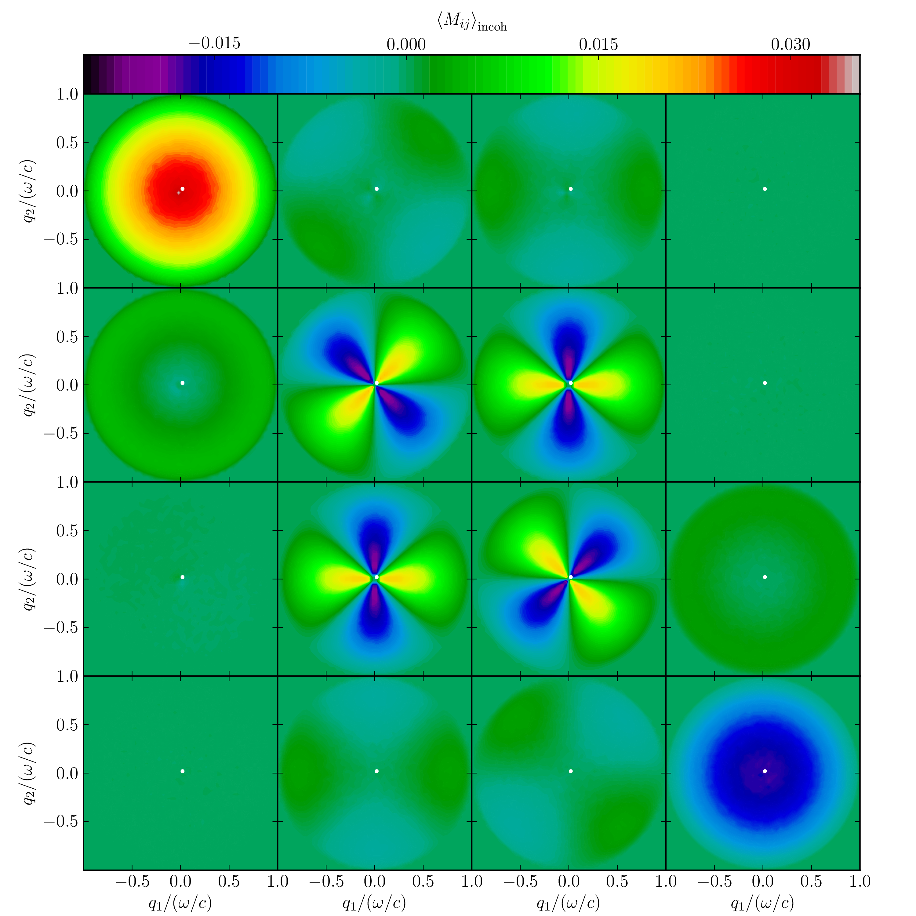
Figure 1: (Color online) Color-level plots of the contribution to the Mueller matrix elements from the light scattered incoherently as functions of $q_{1}$ and $q_{2}$ for angles of incidence $(\theta_{0},\phi_{0})=(2^{\circ},45^{\circ})$. An ensemble consisting of $N_{p}=10\,000$ surface realizations was used in obtaining these results. The elements, $\left<M_{ij}\right>_{\text{incoh}}$ ($i,j=1,2,3,4$), are organized as a matrix with $\left<M_{11}\right>_{\text{incoh}}$ in the top left corner; $\left<M_{12}\right>_{\text{incoh}}$ top row and second column, etc. The white spots indicate the specular direction in reflection.

We have calculated in this way the $16$ elements of the Mueller matrix when light of wavelength $\lambda=457.9$ nm is incident on a two-dimensional randomly rough silver surface whose dielectric function at this wavelength is $\varepsilon(\omega)=-7.5+\mathrm{i}0.24$ Johnson and Christy (1972). The roughness of the surface is defined by a surface height autocorrelation function $W\left(\left|\mathbf{{x}}_{\parallel}\right|\right)=\exp(-x_{\parallel}^{2}/a^{2})$, where $a=\lambda/4$ and the rms height $\delta=\lambda/40$. For the numerical parameters we used $L=25\lambda$ and $N_{x}=319$ which implies that $Q=6.4(\omega/c)$. For these parameters, and when the metal is assumed to be non-absorbing [$\mathrm{Im}\,\varepsilon(\omega)\equiv 0$], our simulation approach conserved energy within a margin of $1$% or better. Moreover, the calculated Mueller matrices were found to be physically realizable and therefore self-consistent by the method of Ref. Cloude (1989).

The results presented in Fig. 1 were obtained for angles of incidence $(\theta_{0},\phi_{0})=(2^{\circ},45^{\circ})$, i.e. for (essentially) normal incidence. The first thing to notice from Fig. 1 is that the individual matrix elements possess the symmetry properties predicted by Bruce Bruce (1998). The elements of the first and last column are circularly symmetric; each element of the second and third columns is invariant under a combined $90^{\circ}$ rotation about the origin and a change of sign; and the elements of the second column are $45^{\circ}$ rotations of the elements of the third column in the same row 222It should be noted that the scattering amplitudes $f_{sp}$ and $f_{ps}$ in Bruce’s Eq. (1) corresponds to our $R_{ps}$ and $R_{sp}$, respectively.. Note that the elements $\left<M_{31}\right>_{\text{incoh}}$, $\left<M_{41}\right>_{\text{incoh}}$, $\left<M_{14}\right>_{\text{incoh}}$, and $\left<M_{24}\right>_{\text{incoh}}$ are zero to the precision used in this calculation. However, simulations indicate that this does not hold for anisotropic surfaces.

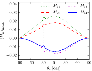
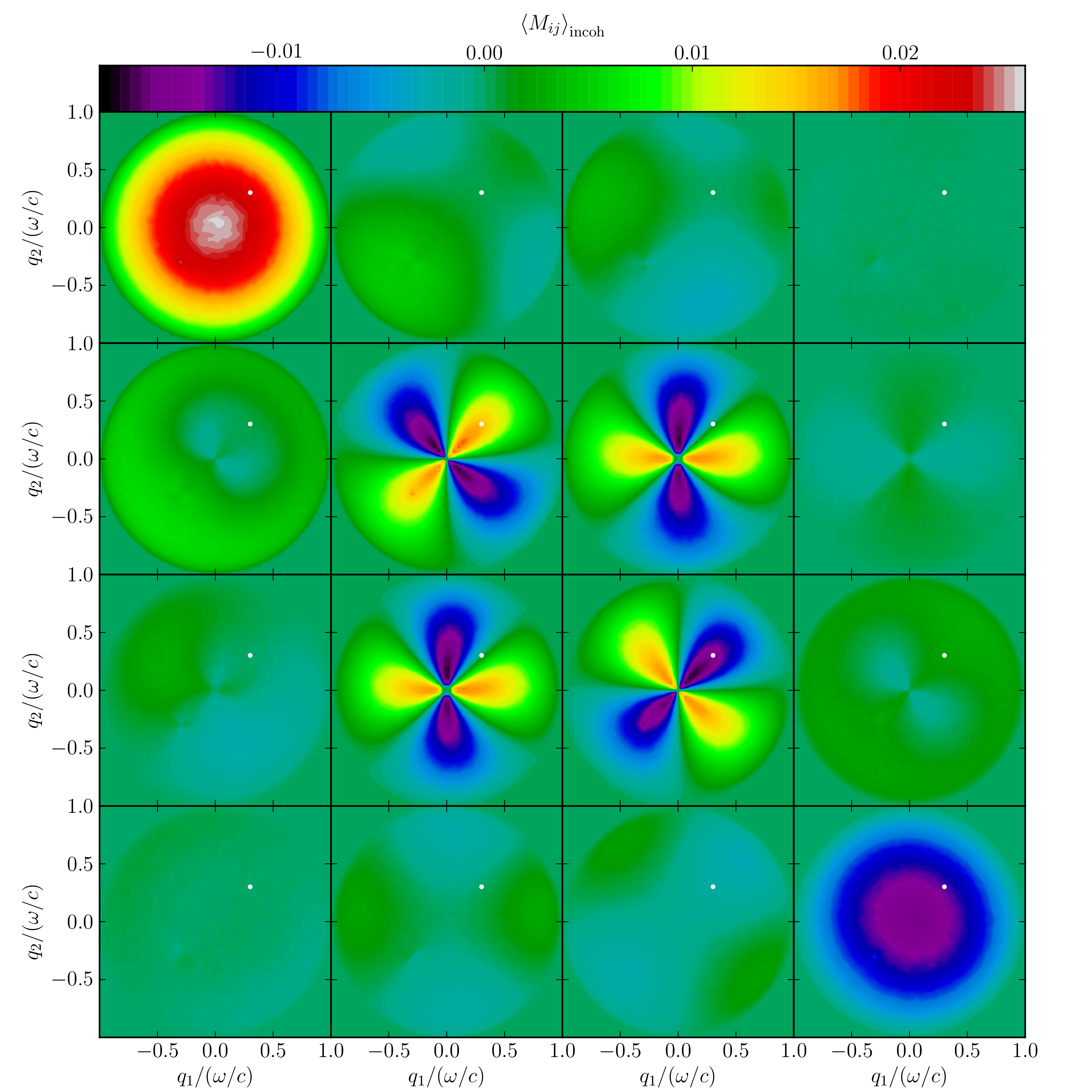
The results presented in Fig. 3 were obtained for angles of incidence $(\theta_{0},\phi_{0})=(25^{\circ},45^{\circ})$, and display some interesting features. The elements $\left<M_{11}\right>_{\text{incoh}}$, $\left<M_{22}\right>_{\text{incoh}}$, and $\left<M_{33}\right>_{\text{incoh}}$ contain a (weak) enhanced backscattering peak at $\mathbf{{q}}_{\parallel}=-\mathbf{{k}}_{\parallel}$ (Fig. 2). The element $\left<M_{44}\right>_{\text{incoh}}$ appears to have a dip in the retroreflection direction. This dip is not present in the results of a calculation based on small-amplitude perturbation theory to the lowest (second) order in the surface profile function, and is therefore a multiple scattering effect, just as the enhanced backscattering peak is. In contrast to what was the case for normal incidence, the elements $\left<M_{31}\right>_{\text{incoh}}$ and $\left<M_{24}\right>_{\text{incoh}}$ are no longer zero.

Refer to caption
Figure 2: The incoherent contribution to the diagonal Mueller matrix elements in the plane of incidence (parameters as in Fig. 3). The vertical dotted line indicates the backscattering direction.
Refer to caption
Figure 3: (Color online) Same as Fig. 1, but now for angles of incidence $(\theta_{0},\phi_{0})=(25^{\circ},45^{\circ})$.

If we denote the ensemble average of the contribution to a normalized element of the Mueller matrix from the light that has been scattered incoherently by $m_{ij}=\left<M_{ij}\right>_{\text{incoh}}/\left<M_{11}\right>_{\text{incoh}}$, we can estimate the order of magnitude of the Mueller matrix elements by calculating the quantities $s_{ij}=\left<|m_{ij}(\mathbf{{q}}_{\parallel})|\right>_{\mathbf{{q}}_{\parallel}}$, where $\left<f(\mathbf{{q}}_{\parallel})\right>_{\mathbf{{q}}_{\parallel}}=\int\!\mathrm{d}^{2}q_{\parallel}\,f(\mathbf{{q}}_{\parallel})/\pi(\omega/c)^{2}$, and the integral over $\mathbf{{q}}_{\parallel}$ is taken over the circular region $0<q_{\parallel}<\omega/c$. It was found that $s_{11}$, $s_{22}$, $s_{23}$, $s_{32}$, $s_{33}$, $s_{44}$ are of ${\mathcal{O}}(1)$; $s_{12}$, $s_{13}$, $s_{21}$, $s_{34}$, $s_{42}$, $s_{43}$ are of ${\mathcal{O}}(0.1)$; and $s_{14}$, $s_{24}$, $s_{31}$, $s_{41}$ are of ${\mathcal{O}}(0.01)$. These results are only weakly dependent on the polar angle of incidence $\theta_{0}$, for the values of $\theta_{0}$ assumed in this study.

In conclusion, we have presented a new approach to the calculation of all sixteen elements of the Mueller matrix for light scattered from a two-dimensional, randomly rough, lossy metal surface, for arbitrary values of the polar and azimuthal angles of incidence. It is based on a rigorous numerical solution of the reduced Rayleigh equation for the scattering of p- and s-polarized light from a two-dimensional rough surface of a penetrable medium, that captures multiple-scattering processes of all orders. The results display multiple scattering effects in certain matrix elements, such as an enhanced backscattering peak in the retroreflection direction, or an unexpected dip in the same direction. The matrix elements also display symmetry properties that, for normal incidence, agree with those predicted by Bruce Bruce (1998).

The physical implications of the approach and results of this Letter point to better understanding of the polarimetric properties of random surfaces. Such knowledge may be critical for improved photovoltaic and remote sensing applications and has the potential of being used to engineer surface structures with well-defined polarization properties of the light interacting with them.

Acknowledgements.
The authors are grateful for fruitful interactions with M. Lindgren, M. Kildemo, I.S. Nerbø, and L.M. Sandvik Aas. The research of P.A.L., T.N., and I.S. was supported in part by NTNU by the allocation of computer time. The research of A.A.M. was supported in part by AFRL contract FA9453-08-C-0230.

References

  • Germer (2007) T. A. Germer, in Light Scattering and Nanoscale Surface Roughness, edited by A. A. Maradudin (Springer, 2007) pp. 259–284.
  • Drezet et al. (2008) A. Drezet, C. Genet, J.-Y. Laluet,  and T. W. Ebbesen, Opt. Express 16, 12559 (2008).
  • Kullock et al. (2008) R. Kullock, W. R. Hendren, A. Hille, S. Grafström, P. R. Evans, R. J. Pollard, R. Atkinson,  and L. M. Eng, Opt. Express 16, 21671 (2008).
  • Schmidt et al. (2011) D. Schmidt, C. Müller, T. Hofmann, O. Inganäs, H. Arwin, E. Schubert,  and M. Schubert, Thin Solid Films 519, 2645 (2011).
  • Martin et al. (2010) W. Martin, E. Hesse, J. Hough, W. Sparks, C. Cockell, Z. Ulanowski, T. Germer,  and P. Kaye, J. Quant. Spectrosc. Ra. 111, 2444 (2010).
  • Ghadyani et al. (2011) Z. Ghadyani, I. Vartiainen, I. Harder, W. Iff, A. Berger, N. Lindlein,  and M. Kuittinen, Appl. Opt. 50, 2451 (2011).
  • Ellis et al. (2002) J. Ellis, P. Caillard,  and A. Dogariu, J. Opt. Soc. Am. A 19, 43 (2002).
  • Mueller (1948) H. Mueller, J. Opt. Soc. Am. 38, 661 (1948).
  • Bickel and Bailey (1985) W. S. Bickel and W. M. Bailey, Am. J. Phys. 53, 468 (1985).
  • Chipman (1994) R. A. Chipman, Handbook of Optics (McGraw–Hill, New York, 1994).
  • Simonsen et al. (2010a) I. Simonsen, A. A. Maradudin,  and T. A. Leskova, Phys. Rev. A 81, 013806 (2010a).
  • Simonsen et al. (2010b) I. Simonsen, A. A. Maradudin,  and T. A. Leskova, Phys. Rev. Lett. 104, 223904 (2010b).
  • (13) T. Nordam, P. A. Letnes,  and I. Simonsen (unpublished) .
  • Simonsen et al. (2011) I. Simonsen, J. B. Kryvi, A. A. Maradudin,  and T. A. Leskova, Comput. Phys. Commun. 182, 1904 (2011).
  • Bruce (1998) N. C. Bruce, Wave. Random Media 8, 15 (1998).
  • Zhang and Bahar (1999) Y. Zhang and E. Bahar, IEEE Trans. Antennas Propag. 47, 949 (1999).
  • Brown et al. (1984) G. Brown, V. Celli, M. Haller,  and A. Marvin, Surf. Sci. 136, 381 (1984).
  • Maradudin et al. (1990) A. A. Maradudin, T. Michel, A. R. McGurn,  and E. R. Mendez, Ann. Phys. 203, 255 (1990).
  • Press et al. (1992) W. H. Press, S. A. Teukolsky, W. T. Vetterling,  and B. P. Flannery, Numerical Recipes in C, 2nd ed. (Cambridge University Press, 1992).
  • Note (1) A. A. Maradudin (unpublished).
  • Johnson and Christy (1972) P. B. Johnson and R. W. Christy, Phys. Rev. B 6, 4370 (1972).
  • Cloude (1989) S. R. Cloude, Proc. SPIE 1166, 177 (1989).
  • Note (2) It should be noted that the scattering amplitudes $f_{sp}$ and $f_{ps}$ in Bruce’s Eq. (1) corresponds to our $R_{ps}$ and $R_{sp}$, respectively.