Quantum fidelity for one-dimensional Dirac fermions and two-dimensional Kitaev model in the thermodynamic limit

Abstract

We study the scaling behavior of the fidelity ($F$) in the thermodynamic limit using the examples of a system of Dirac fermions in one dimension and the Kitaev model on a honeycomb lattice. We show that the thermodynamic fidelity inside the gapless as well as gapped phases follow power-law scalings, with the power given by some of the critical exponents of the system. The generic scaling forms of $F$ for an anisotropic quantum critical point for both thermodynamic and non-thermodynamic limits have been derived and verified for the Kitaev model. The interesting scaling behavior of $F$ inside the gapless phase of the Kitaev model is also discussed. Finally, we consider a rotation of each spin in the Kitaev model around the $z$ axis and calculate $F$ through the overlap between the ground states for angle of rotation $\eta$ and $\eta+d\eta$, respectively. We thereby show that the associated geometric phase vanishes. We have supplemented our analytical calculations with numerical simulations wherever necessary.

I Introduction

A quantum phase transition chakrabarti96 ; sachdev99 ; continentino ; sondhi97 ; vojta03 driven exclusively by quantum fluctuations at zero temperature is associated with a dramatic change in the symmetry of the ground state of a many-body quantum Hamiltonian. A number of measures from quantum information theory such as entanglement osterloh02 ; roncaglia06 , entanglement entropy vidal03 ; kitaev061 , Loschmidt echo song06 , decoherence damski10 and quantum discord olliver01 ; dillenschneider08 are able to capture the singularities associated with a quantum critical point (QCP). Consequently, there is a recent upsurge in the investigation of quantum critical systems from the perspective of quantum information theory in an attempt to establish a bridge between these two fields amico08 ; latorre09 ; duttarmp10 .

An important information theoretic concept that is being investigated extensively for quantum critical systems is the quantum fidelity ($F$) zanardi06 ; venuti07 ; giorda07 ; zhou081 ; shigu08 ; gurev10 ; schwandt09 ; gritsev09 ; yang08 ; lin09 ; grandi10 ; polkovnikovrmp ; mukherjee10 ; mukherjee11 ; zhou082 ; zhou083 ; zhao09 ; znidaric03 ; ma08 ; eriksson09 ; rams11 . Let us consider a $d$-dimensional Hamiltonian $H(\lambda)$ which contains an externally tunable parameter $\lambda$, such that the system is at a QCP when $\lambda=0$. Considering two ground state wave functions $|\psi_{0}(\lambda)\rangle$ and $|\psi_{0}(\lambda+\delta)\rangle$, which are infinitesimally separated in the parameter space as $\delta\to 0$, we define the fidelity as

$$F(\lambda,\lambda+\delta) = |\langle\psi_{0}(\lambda)|\psi_{0}(\lambda+\delta)\rangle|$$ (1)

$$= 1-\frac{\delta^{2}}{2}L^{d}\chi_{F}+\cdots,$$

where $L$ is the linear dimension of the system, and $\delta$ denotes a small change in the parameter $\lambda$. The first non-vanishing term in the expansion of $F$, namely, the fidelity susceptibility $\chi_{F}$, provides a quantitative measure of the rate of change of the ground state under an infinitesimal variation of $\lambda$. By exhibiting a sharp decay around a QCP even for a finite size system, the fidelity turns out to be one of the fundamental probes for detecting the ground state singularities associated with a quantum phase transition without making reference to an order parameter. At the same time, the fidelity susceptibility defined through the relation $\chi_{F}=-(2/L^{d})(\ln F)/\delta^{2}|_{\delta\to 0}=-(1/L^{d})(\partial^{2}F/\partial\delta^{2})$ usually diverges with the system size in a universal power-law fashion with an exponent given in terms of some of the quantum critical exponents. For a marginal or relevant perturbation $\lambda$, the application of the adiabatic perturbation theory leads to a generic scaling form venuti07 ; gurev10 ; gritsev09 ; schwandt09 ; grandi10 of $\chi_{F}$ given by $\chi_{F}(\lambda=0)\sim L^{2/\nu-d}$ at the QCP, whereas away from the QCP, the scaling changes to $\chi_{F}\sim|\lambda|^{\nu d-2}$ for $L>\lambda^{-\nu}$; here $\nu$ is the critical exponent describing the divergence of the spatial correlation length close to the QCP, i.e., $\xi\sim\lambda^{-\nu}$.

While the fidelity susceptibility approach usually assumes small $L$ and $\delta\to 0$, the fidelity per sitezhou082 ; zhou083 ; zhao09 has been calculated in the thermodynamic limit for an arbitrary value of $\delta$ in some recent studies zhou082 ; zhou083 ; zhao09 . In such cases, the fidelity differs significantly from unity unlike in Eq. (1). The fidelity per site is also able to indicate the appearance of a quantum phase transition in the spin-1/2 $XY$ model in a transverse magnetic field. Another measure of fidelity applied to mixed states, namely, the reduced fidelity znidaric03 ; ma08 ; eriksson09 has also provided important insights into quantum critical phenomena. We note that similar studies have been carried out on the scaling of the geometric phase pancharatnam56 ; berry84 which is closely related to the fidelity susceptibilityvenuti07 close to critical carollo05 ; zhu06 ; hamma06 and multicritical patra11 points.

As seen from Eq. (1) and also the preceding discussion, the knowledge of $\chi_{F}$ should be sufficient to draw conclusions about the behavior of $F$ and the associated QCP for small system sizes and in the limit $\delta\to 0$ ($\delta^{2}L^{d}\chi_{F}/2\ll 1$). However, in the thermodynamic limit ($L\to\infty$ at fixed $\delta$), the expansion in Eq. (1) up to the lowest order becomes insufficient. Recently, Rams and Damski rams11 have proposed a generic scaling relation rams11 valid in the thermodynamic limit given by

$$\ln{F(\lambda-\delta,\lambda+\delta)}\simeq-L^{d}|\delta|^{\nu d}A\left(\frac{\lambda}{|\delta|}\right),$$ (2)

where $A$ is a scaling function; this relation interpolates between the fidelity susceptibility approach and the fidelity per site approach. In deriving the scaling relation in Eq. (2), it is assumed that the fidelity per site is well behaved in the limit $L\to\infty$, the QCP is determined by a single set of critical exponents, and $\nu d>2$ so that non-universal corrections are subleading gritsev09 . In particular, at the critical point $\lambda=0$, the fidelity, measured between the ground states at $+\delta$ and $-\delta$, is non-analytic in $\delta$ and satisfies the scaling $\ln{F}\sim-L^{d}|\delta|^{\nu d}$. On the other hand, away from the QCP, i.e., for $|\delta|\ll|\lambda|\ll 1$, the scaling gets modified to $\ln{F}\sim-L^{d}\delta^{2}|\lambda|^{\nu d-2}$. This scaling has been verified for an isolated quantum critical point using one-dimensional transverse Ising and $XY$ Hamiltonians rams11 . Moreover, near a QCP a cross-over has been observed from the thermodynamic limit ($L|\delta|^{\nu}\gg 1$) to the non-thermodynamic (small system) limit ($L|\delta|^{\nu}\ll 1$) where the concept of fidelity susceptibility becomes useful. We note that Eq. (2) is an example of the Anderson orthogonality catastrophe anderson67 which states that the overlap of two states vanishes in the thermodynamic limit irrespective of their proximity to a QCP.

In this paper we investigate the scaling of the thermodynamic fidelity in a one-dimensional system of Dirac fermions with a mass perturbation mahan00 ; gogolin98 ; vondelft98 ; giamarchi04 ; giuliani05 and the two-dimensional Kitaev model on a honeycomb lattice kitaev06 ; chen07 close to or inside the gapless phases of their phase diagrams, thereby extending previous studies to more generic situations. For the one-dimensional system, we have verified the scaling predicted in Ref. rams11, . We also propose a generic scaling form for the thermodynamic fidelity in the vicinity of an anisotropic quantum critical point (AQCP), and we verify it for the AQCP present in the Kitaev model phase diagram hikichi10 .

The paper is organized in the following way. In Sec. II, we analytically derive the scaling relations of the thermodynamic fidelity for non-interacting spinless massive Dirac fermions in one dimension and propose a generalization to the case of interacting fermions (called a Tomonaga-Luttinger liquid). In Sec. III, we concentrate on the fidelity of the Kitaev model on the hexagonal lattice for different values of the coupling parameters. We derive the scaling laws for both the thermodynamic and non-thermodynamic limits for an AQCP and verify these numerically for the Kitaev model. In Sec. IV, we calculate the overlap between two ground states of the Kitaev model; in one state, all the spins are rotated about the $z$ axis by an angle $\eta$, while in the other, they are rotated by an angle $\eta+d\eta$. We thus derive the form of the fidelity through an expansion in powers of $d\eta$.

II Dirac fermions in one dimension

In this section we consider a system of spinless Dirac fermions in one dimension with a mass perturbation and verify the scaling of the thermodynamic fidelity as predicted in Ref. rams11, . Let us first consider non-interacting fermions. The Hamiltonian we consider is

$$H=\sum^{\infty}_{k>0}{\left[k\left(c^{\dagger}_{k}c_{k}-c^{\dagger}_{-k}c_{-k}\right)+m\left(c^{\dagger}_{k}c_{-k}+c^{\dagger}_{-k}c_{k}\right)\right]},$$ (3)

where $c_{k}^{\dagger}$ ($c_{k}$) is the fermionic creation (annihilation) operator for wave vector $k$, $m$ is the mass, and we have set the velocity $v=1$ for convenience. In the two-level system given by $c^{\dagger}_{k}c_{k}+c^{\dagger}_{-k}c_{-k}=1$, the Hamiltonian takes the form

$$H = \sum^{\infty}_{k>0}\left(\begin{array}[]{cc}c^{\dagger}_{k}&c^{\dagger}_{-k}\end{array}\right)h_{k}\left(\begin{array}[]{c}c_{k}\\ c_{-k}\end{array}\right),$$ (7)

$$\text{where}~{}~{}h_{k} = \left(\begin{array}[]{cc}k&m\\ m&-k\end{array}\right).$$ (10)

The normalized ground state of this is given by

$$\psi(k,m)$$ (13)

$$= \frac{1}{\sqrt{2\left(k^{2}+m^{2}\right)+2k\sqrt{k^{2}+m^{2}}}}\left(\begin{array}[]{c}m\\ -\sqrt{k^{2}+m^{2}}-k\end{array}\right).$$

with the energy $E_{k}=-\sqrt{k^{2}+m^{2}}$.

If we now consider two systems with masses $m_{1}$ and $m_{2}$, the fidelity between the two ground states is given by

$$F(m_{1},m_{2})~{}=~{}\prod_{k>0}~{}|\langle\psi(k,m_{1})|\psi(k,m_{2})\rangle|.$$ (15)

Note that we have taken $k$ to be strictly positive in all the equations above. It is important to exclude the mode with $k=0$, otherwise the fidelity is exactly equal to zero if $m_{1}$ and $m_{2}$ have opposite signs; this is because $\langle\psi(0,m_{1})|\psi(0,m_{2})\rangle=0$ if $m_{1}m_{2}<0$. The simplest way to exclude a zero momentum mode is to impose antiperiodic boundary conditions, $\psi(x=L)=-\psi(x=0)$, so that $k_{n}=(\pi/L)(2n+1)$, where $L$ is the system size and $n=0,1,2,\cdots$. (Note that the spacing between successive values of $k$ is $2\pi/L$). We can then write Eq. (15) as

$$F(m_{1},m_{2})~{}=~{}\prod_{n=0}^{\infty}~{}|\langle\psi(k_{n},m_{1})|\psi(k_{n},m_{2})\rangle|.$$ (16)

Now we consider the case with $m_{1}=m$ and $m_{2}=-m$ so that the states lie on the two sides of the gapless critical point, and $m$ plays the role of $\delta$ discussed in the previous section. We find that

$$\langle\psi(k_{n},m)|\psi(k_{n},-m)\rangle=\frac{k_{n}^{2}+k_{n}\sqrt{k_{n}^{2}+m^{2}}}{k_{n}^{2}+m^{2}+k_{n}\sqrt{k_{n}^{2}+m^{2}}}.$$ (17)

Since $k_{n}=(\pi/L)(2n+1)$, we see that the fidelity is a function of a single parameter given by $mL$. We now consider two cases: (i) $mL\gg 1$ and (ii) $mL\ll 1$. In both cases, we will assume that $L\gg 1$. (Cases (i) and (ii) will be respectively called the thermodynamic and non-thermodynamic limits in the next section).

In case (i), we can take $k$ to be a continuous variable so that the fidelity is given by an integral,

$$F(m,-m)=\exp\left[L\int^{\infty}_{0}{\frac{dk}{2\pi}\ln|\langle\psi(k,m_{1})|\psi(k,m_{2})\rangle|}\right],$$ (18)

By writing $k=mx$ in the integral, we find that $F(m,-m)$ is given by $e^{-cmL}$, where

$$c=-\int^{\infty}_{0}{\frac{dx}{2\pi}\ln\left[\frac{x^{2}+x\sqrt{x^{2}+1}}{x^{2}+1+x\sqrt{x^{2}+1}}\right]}.$$ (19)

We conclude that the fidelity satisfies the scaling form $\ln F\sim-cLm$ which is in agreement with the prediction rams11 that $\ln F\sim-cL\delta^{d\nu}$ where $\nu=d=1$ and $m=\delta$ in the present case.

In case (ii), we can expand $\langle\psi(k_{n},m)|\psi(k_{n},-m)\rangle=1~{}-~{}m^{2}L^{2}/[2(2n+1)^{2}]$ to lowest order in $mL$. We then obtain

$$\ln F(m,-m)\simeq-\frac{m^{2}L^{2}}{2}~{}\sum_{n=0}^{\infty}~{}\frac{1}{(2n+1)^{2}}=-\frac{\pi^{2}m^{2}L^{2}}{16}.$$ (20)

Hence we find the scaling relation $\ln F\sim\delta^{2}L^{2/\nu}$ in the non-thermodynamic limit; we can further conclude that $\chi_{F}\sim L^{2/\nu-d}$.

We now consider what happens if the fermions were interacting; in one dimension, such a system is described by Tomonaga-Luttinger liquid theory mahan00 ; gogolin98 ; vondelft98 ; giamarchi04 ; giuliani05 . To be specific, let us consider the spin-1/2 $XXZ$ chain in a transverse magnetic field; the Hamiltonian is given by

$$H = \frac{1}{2}~{}\sum_{n=-\infty}^{\infty}~{}[~{}\sigma_{n}^{x}\sigma_{n+1}^{x}~{}+~{}\sigma_{n}^{y}\sigma_{n+1}^{y}~{}+~{}J_{z}\sigma_{n}^{z}\sigma_{n+1}^{z}$$ (21)

$$~{}~{}~{}~{}~{}~{}~{}~{}~{}~{}~{}~{}~{}-~{}h_{n}\sigma_{n}^{z}~{}].$$

We first set $h_{n}=0$. Upon using the Jordan-Wigner transformation which takes us from spin-1/2 to spinless fermions in one dimension lieb61 , we find that the first two terms in Eq. (21), $(1/2)(\sigma_{n}^{x}\sigma_{n+1}^{x}+\sigma_{n}^{y}\sigma_{n+1}^{y})$, lead to a tight-binding Hamiltonian of the form $-\sum_{n}(c_{n}^{\dagger}c_{n+1}+c_{n+1}^{\dagger}c_{n})$; Fourier transforming to $k$-space, and linearizing around the two Fermi points lying at $k=\pm\pi/2$ gives the first term in Eq. (3). The third term in Eq. (21), $\sigma_{n}^{z}\sigma_{n+1}^{z}$, leads to a four-fermion interaction of the form $c_{n}^{\dagger}c_{n}c_{n+1}^{\dagger}c_{n+1}$. Eq. (21) describes a system of massless interacting fermions if $J_{z}$ lies in the range $-1\leq J_{z}<1$. (The cases $J_{z}=-1$ and $1$ describe an isotropic ferromagnet and isotropic antiferromagnet respectively). The system is characterized by a Luttinger parameter $K$ given by

$$K~{}=~{}\frac{\pi}{2\cos^{-1}(-J_{z})},$$ (22)

so that $K$ goes from $\infty$ to $1/2$ as $J_{z}$ goes from $-1$ to 1. If $J_{z}=0$, there are no interactions between the fermions and we obtain $K=1$.

We now introduce an alternating magnetic field of the form $h_{n}=m(-1)^{n}$; this introduces a coupling between the modes at the Fermi points $k=\pm\pi/2$ and therefore gives rise to the mass term in Eq. (3) if $J_{z}=0$ ($K=1$). The most efficient way of studying the low-energy, long wavelength modes (i.e., the modes near the Fermi points) of a one-dimensional system of interacting fermions ($K\neq 1$) is to use the technique of bosonization mahan00 ; gogolin98 ; vondelft98 ; giamarchi04 ; giuliani05 . Bosonization uses a quantum field theory which is defined in terms of a scalar field $\phi$. In this description, the action is given by

$$S~{}=~{}\frac{1}{2K}\int\int dtdx~{}\left[~{}\left(\frac{\partial\phi}{\partial t}\right)^{2}~{}-~{}\left(\frac{\partial\phi}{\partial x}\right)^{2}\right]$$ (23)

for $m=0$ (we have again set the velocity equal to 1); the effect of interactions appears through the Luttinger parameter $K$. The contribution of the mass term to the action takes the form

$$S_{m}~{}\sim~{}\int\int dtdx~{}m~{}\cos(2\sqrt{\pi}\phi).$$ (24)

The operator $\cos(2\sqrt{\pi}\phi)$ is known to have mass dimension $K$; let us denote the coefficient of this operator in the action by $\lambda$. It turns out that $\lambda$ effectively becomes dependent on the length scale $L$, and $\lambda(L)$ satisfies the renormalization group (RG) equation $d\lambda/d\ln L=(2-K)\lambda$. Given the initial value of $\lambda(a)=m$ at some microscopic length scale $a$ (such as the lattice spacing), and assuming that $m\ll 1$, the RG equation implies that $\lambda(L)$ grows and becomes of order 1 at a length scale given by $\xi$, where $\xi/a\sim 1/m^{1/(2-K)}$. Hence the mass gap of the theory is given by $1/\xi\sim m^{1/(2-K)}$, leading to a low-energy dispersion given by $\omega_{k}=\sqrt{k^{2}+m^{2/(2-K)}}$. One can then argue qualitatively that our above arguments about fidelity would remain valid, but with a renormalized mass term given by $m^{1/(2-K)}$. For case (i) where $Lm^{1/(2-K)}\gg 1$, we would eventually find that the fidelity scales as $\ln F(m,-m)\sim-c^{{}^{\prime}}Lm^{1/(2-K)}$, where $c^{\prime}$ is a prefactor which differs from $c$ due to the presence of the interactions. Noting that the correlation length exponent in the presence of the mass perturbation is $\nu=1/(2-K)$, we find that the scaling in Eq. (2) should also hold good, with $d=1$ and $\delta=m$. The above analysis is only valid for $K<2$; for $K>2$, the mass perturbation is irrelevant in the sense of the renormalization group, and the fidelity has to be calculated in some other way which we will not pursue here.

We will not examine here the effects of a perturbation which takes the system across a Kosterlitz-Thouless transition; this occurs if $h_{n}=0$ and $J_{z}$ crosses 1. The fidelity across this transition is considerably harder to analyze, and we refer to the work done by different groups yang07 ; fjaerstad08 ; chen08 ; sirker10 ; wang11 .

III Kitaev Model

In this section, we will exploit the solvability of the Kitaev model on the honeycomb lattice kitaev06 to calculate the fidelity of the model as a function of various parameters in the thermodynamic limit. We note that the fidelity per site studied for the same model has been able to detect quantum phase transitions zhao09 , and the fidelity susceptibility has been calculated previously in the limit of small system sizes yang08 ; lin09 .

III.1 Model, phase diagram and fidelity

The Hamiltonian of the Kitaev model is given by

$$H=\sum_{j+l=even}~{}(J_{1}\sigma_{j,l}^{x}\sigma_{j+1,l}^{x}+J_{2}\sigma_{j-1,l}^{y}\sigma_{j,l}^{y}+J_{3}\sigma_{j,l}^{z}\sigma_{j,l+1}^{z}),$$ (25)

where $j$ and $l$ respectively denote the column and row indices of a honeycomb lattice (see Fig. 1) kitaev06 ; hikichi10 ; chen07 ; sengupta08 . We will assume that the couplings $J_{i}$, for $i=1,2,3$, are all positive; if some of them are negative, they can be made positive by appropriate $\pi$ rotations about the $x$, $y$ or $z$ spin axis. For the moment, our study will be restricted to the case $J_{1}=J_{2}$, although we will comment on the case with $J_{1}\neq J_{2}$ in Sec. III E.

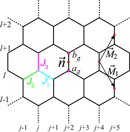
Figure 1: (Color online) Schematic representation of the Kitaev model on a honeycomb lattice showing the bonds with couplings $J_{1}$, $J_{2}$ and $J_{3}$. $\vec{M}_{1}$ and $\vec{M}_{2}$ are spanning vectors of the lattice. Sites ‘$a_{\vec{n}}$’ and ‘$b_{\vec{n}}$’ represent the two inequivalent sites which make up a unit cell. (After reference [hikichi10, ])

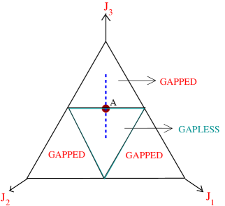
Figure 2: (Color online) Phase diagram of the Kitaev model; all the points in the triangle satisfy $J_{1}+J_{2}+J_{3}=1$. The gapless phase is the region in which the couplings satisfy the triangle inequalities given by $J_{1}\leq J_{2}+J_{3}$, $J_{2}\leq J_{3}+J_{1}$ and $J_{3}\leq J_{1}+J_{2}$, i.e., the points inside the inner equilateral triangle. Along the dashed vertical line $J_{3}$ is varied holding $J_{1}=J_{2}$, and the anisotropic quantum critical point (A) at $J_{3}=J_{3,c}=J_{1}+J_{2}=2J_{1}$ is indicated. Our focus is to calculate the fidelity between ground states lying on this vertical line.

We define the Jordan-Wigner transformation as

$$a_{j,l} = \left(\prod_{i=-\infty}^{j-1}\sigma_{i,l}^{z}\right)\sigma_{j,l}^{y}~{}~{}~{}\text{for even}~{}~{}j+l,$$

$$a^{\prime}_{j,l} = \left(\prod_{i=-\infty}^{j-1}\sigma_{i,l}^{z}\right)\sigma_{j,l}^{x}~{}~{}~{}\text{for even}~{}~{}j+l,$$

$$b_{j,l} = \left(\prod_{i=-\infty}^{j-1}\sigma_{i,l}^{z}\right)\sigma_{j,l}^{x}~{}~{}~{}\text{for odd}~{}~{}j+l,$$

$$b^{\prime}_{j,l} = \left(\prod_{i=-\infty}^{j-1}\sigma_{i,l}^{z}\right)\sigma_{j,l}^{y}~{}~{}~{}\text{for odd}~{}~{}j+l,$$ (26)

where $a_{j,l}$, $a^{\prime}_{j,l}$, $b_{j,l}$ and $b^{\prime}_{j,l}$ are all Majorana fermions, i.e., they are Hermitian, their square is equal to 1, and they anticommute with each other. Instead of using the indices $(j,l)$ to specify the sites, we can use the two-dimensional vectors $\vec{n}=\sqrt{3}\hat{i}n_{1}+(\frac{\sqrt{3}}{2}\hat{i}+\frac{3}{2}\hat{j})n_{2}$ which denote the midpoints of the vertical bonds of the honeycomb lattice; here $\hat{i}$ denotes the unit vector along the horizontal (labeled by $j,~{}j+1$, etc) and similarly $\hat{j}$ is the unit vector along the vertical direction. Here $n_{1}$ and $n_{2}$ run over all integers so that the vectors $\vec{n}$ form a triangular lattice. The Majorana fermions $a_{\vec{n}}$ ($a^{\prime}_{\vec{n}}$) and $b_{\vec{n}}$ ($b^{\prime}_{\vec{n}}$) are located at the bottom and top lattice sites respectively of the bond labeled by $\vec{n}$. The vectors $\vec{M_{1}}=\frac{\sqrt{3}}{2}\hat{i}-\frac{3}{2}\hat{j}$ and $\vec{M_{2}}=\frac{\sqrt{3}}{2}\hat{i}+\frac{3}{2}\hat{j}$ shown in Fig. 1 are the spanning vectors of the lattice. (We have set the nearest neighbor lattice spacing to unity).

The Fourier transforms of the Majorana fermions are given by

$$a_{\vec{n}}~{}=~{}\sqrt{\frac{4}{L}}~{}\sum_{\vec{k}}~{}[~{}a_{\vec{k}}~{}e^{i{\vec{k}}\cdot{\vec{n}}}~{}+~{}a_{\vec{k}}^{\dagger}~{}e^{-i{\vec{k}}\cdot{\vec{n}}}~{}],$$ (27)

satisfying $\{a_{\vec{k}},a^{\dagger}_{\vec{k}^{\prime}}\}=\delta_{{\vec{k}},{\vec{k}^{\prime}}}$, and similarly for $a^{\prime}_{\vec{n}}$, $b_{\vec{n}}$ and $b^{\prime}_{\vec{n}}$. In Eq. (27), $L$ is the number of sites (hence the number of unit cells is $L/2$), and the sum over $\vec{k}$ extends over half the Brillouin zone of the hexagonal lattice because of the Majorana nature of the fermions chen07 ; sengupta08 . The full Brillouin zone is given by a rhombus with vertices lying at $(k_{x},k_{y})=(\pm 2\pi/\sqrt{3},0)$ and $(0,\pm 2\pi/3)$; half the Brillouin zone is given by an equilateral triangle with vertices at $(k_{x},k_{y})=(2\pi/\sqrt{3},0)$ and $(0,\pm 2\pi/3)$.

In terms of the Majorana fermions, the Hamiltonian in Eq. (25) takes the form

$$H^{\prime}=i\sum_{\vec{n}}\left(J_{1}b_{\vec{n}}a_{\vec{n}-\vec{M_{1}}}+J_{2}b_{\vec{n}}a_{\vec{n}+\vec{M_{2}}}+J_{3}D_{\vec{n}}b_{\vec{n}}a_{\vec{n}}\right),$$ (28)

where $D_{\vec{n}}=i~{}b^{\prime}_{\vec{n}}a^{\prime}_{\vec{n}}$. We note that the operators $D_{\vec{n}}$ have eigenvalues $\pm 1$, and commute with each other and with $H^{\prime}$; hence all the eigenstates of $H^{\prime}$ can be labeled by specific values of $D_{\vec{n}}$. (We observe that the Hamiltonian $H^{\prime}$ gives dynamics to the fermions $a_{\vec{n}}$ and $b_{\vec{n}}$, but the fermions $a^{\prime}_{\vec{n}}$ and $b^{\prime}_{\vec{n}}$ have no dynamics since $ib^{\prime}_{\vec{n}}a^{\prime}_{\vec{n}}$ is fixed). The ground state can be shown to correspond to $D_{\vec{n}}=1$ for all ${\vec{n}}$. kitaev06 For $D_{\vec{n}}=1$, the Hamiltonian can be diagonalized into the form

$$H^{\prime}=\sum_{\vec{k}}~{}\left(\begin{array}[]{cc}a^{\dagger}_{\vec{k}}&b^{\dagger}_{\vec{k}}\end{array}\right)~{}H_{\vec{k}}~{}\left(\begin{array}[]{c}a_{\vec{k}}\\ b_{\vec{k}}\end{array}\right),$$ (29)

where $H_{\vec{k}}$ can be written in terms of Pauli matrices as

$$H_{\vec{k}} = \alpha_{\vec{k}}~{}\sigma^{1}~{}+~{}\beta_{\vec{k}}~{}\sigma^{2},$$

$${\rm where}~{}~{}\alpha_{\vec{k}} = 2[J_{1}\sin(\vec{k}\cdot\vec{M_{1}})-J_{2}\sin(\vec{k}\cdot\vec{M_{2}})],$$

$${\rm and}~{}~{}\beta_{\vec{k}} = 2[J_{3}+J_{1}\cos(\vec{k}\cdot\vec{M_{1}})+J_{2}\cos(\vec{k}\cdot\vec{M_{2}})].$$

The energy spectrum of $H^{\prime}$ consists of two bands with energies given by

$$E^{\pm}_{\vec{k}}~{}=~{}\pm~{}\sqrt{\alpha^{2}_{\vec{k}}~{}+~{}\beta^{2}_{\vec{k}}}.$$ (31)

The energy gap $E^{+}_{\vec{k}}-E^{-}_{\vec{k}}$ vanishes for specific values of $\vec{k}$ when $|J_{1}-J_{2}|\leq J_{3}\leq J_{1}+J_{2}$ giving rise to a gapless phase of the model. The gapless and gapped phases of the model are shown in Fig. 2 in terms of points in an equilateral triangle which satisfy $J_{1}+J_{2}+J_{3}=1$ and all $J_{i}>0$, with the value of $J_{i}$ being given by the distance from the opposite side of the triangle as indicated by the arrows. In the limit $J_{3}=0$, the Hamiltonian (25) reduces to a one-dimensional version of the Kitaev model feng07 which in turn can be mapped to the transverse Ising chain following a duality transformation capel77 .

In particular, let us consider the critical line $J_{3}=J_{1}+J_{2}$ which separates one of the gapped phases from the gapless phase in Fig. 2. On this line, the energy vanishes at the three corners of half the Brillouin zone given by ${\vec{k}}=(2\pi/\sqrt{3},0)$ and $(0,\pm 2\pi/3)$; these three points are actually equivalent to each other because they are related by shifts by the lattice vectors $G_{\pm}=(2\pi/\sqrt{3},\pm 2\pi/3)$. If $(dk_{x},dk_{y})$ denotes a small deviation from any one of these three points, we find that the energy is highly anisotropic with respect to this deviation. Namely, for $J_{3}=J_{1}+J_{2}$, the quantities $\alpha_{\vec{k}}$ and $\beta_{\vec{k}}$ appearing in Eqs. (LABEL:hamilreduced-31) are given by

$$\alpha_{\vec{k}} = \sqrt{3}(J_{2}-J_{1})dk_{x}+3(J_{1}+J_{2})dk_{y},$$

$$\beta_{\vec{k}} = J_{1}\left(\frac{\sqrt{3}}{2}dk_{x}-\frac{3}{2}dk_{y}\right)^{2}+J_{2}\left(\frac{\sqrt{3}}{2}dk_{x}+\frac{3}{2}dk_{y}\right)^{2},$$

respectively, to lowest order in $dk_{x}$ and $dk_{y}$. We see that $\alpha_{\vec{k}}$ varies linearly in one particular direction in the plane of $(dk_{x},dk_{y})$, while $\beta_{\vec{k}}$ varies quadratically in any direction. We thus have an AQCP hikichi10 . For simplicity, we will mainly restrict our attention below to the case where $J_{1}=J_{2}$ is held fixed and $J_{3}$ is varied along the dashed vertical line shown in Fig. 2. Then the point $J_{3}=J_{3,c}=2J_{1}$ marked by $A$ is an AQCP, with the energy gap vanishing near the three points as $E_{\vec{k}}\sim(dk_{x})^{2}$ and $dk_{y}$ for deviations along the $k_{x}$ and $k_{y}$ directions respectively. For $J_{1}=J_{2}$, the dispersion is linear along the vertical direction $\hat{j}$ and quadratic along the horizontal direction $\hat{i}$ (see Fig. 1). This implies, for the analysis given in Sec. III B, that the correlation length exponent $\nu_{\perp}=1$ and $L_{\perp}$ is the length of the system in the $\hat{j}$ direction, while the exponent $\nu_{||}=1/2$ and $L_{||}$ is the length of the system in the $\hat{i}$ direction. For a more general AQCP given by $J_{3}=J_{1}+J_{2}$ but $J_{1}\neq J_{2}$, Eq. (LABEL:disp) implies that the dispersion is linear along a direction given by ${\hat{e}}_{1}=\sqrt{3}(J_{2}-J_{1}){\hat{i}}+3(J_{1}+J_{2}){\hat{j}}$ and quadratic in a direction ${\hat{e}}_{2}$ which is perpendicular to ${\hat{e}}_{1}$. Hence $\nu_{\perp}=1$ and $L_{\perp}$ is the length of the system in the ${\hat{e}}_{1}$ direction, while $\nu_{||}=1/2$ and $L_{||}$ is the length of the system in the ${\hat{e}}_{2}$ direction.

We will now show that the ground state of the model in Eq. (28) can be written as a product over all $\vec{k}$ lying in half the Brillouin zone. Firstly, the unprimed Majorana fermions $a_{\vec{k}}$ and $b_{\vec{k}}$ must be chosen to have the lower eigenvalue $E^{-}_{\vec{k}}$ of $H_{\vec{k}}$; the corresponding normalized state is given by

$$|S_{\vec{k}}\rangle = (1/\sqrt{2})~{}(~{}a^{\dagger}_{\vec{k}}~{}-~{}e^{i\theta_{\vec{k}}}~{}b^{\dagger}_{\vec{k}})~{}|\Phi\rangle,$$

$${\rm where}~{}~{}e^{i\theta_{\vec{k}}} = \frac{\alpha_{\vec{k}}~{}+~{}i\beta_{\vec{k}}}{\sqrt{\alpha^{2}_{\vec{k}}~{}+~{}\beta^{2}_{\vec{k}}}},$$ (33)

and $|\Phi\rangle$ is the vacuum state annihilated by $a_{\vec{k}}$, $a^{\prime}_{\vec{k}}$, $b_{\vec{k}}$ and $b^{\prime}_{\vec{k}}$. Secondly, the condition $D_{\vec{n}}=ib^{\prime}_{\vec{n}}a^{\prime}_{\vec{n}}=1$ for all $\vec{n}$ implies that if we define the Dirac fermion operators $c_{\vec{n}}=(1/2)(a^{\prime}_{\vec{n}}-ib^{\prime}_{\vec{n}})$, the ground state must be an eigenstate of $c^{\dagger}_{\vec{n}}c_{\vec{n}}$ with eigenvalue 1 for all $\vec{n}$. Hence the state must be annihilated by $c^{\dagger}_{\vec{n}}$ for all $\vec{n}$; taking the Fourier transform of this means that the state must be annihilated by both $c^{\dagger}_{\vec{k}}=(1/2)(a^{\prime\dagger}_{\vec{k}}+ib^{\prime\dagger}_{\vec{k}})$ and $c_{\vec{k}}=(1/2)(a^{\prime}_{\vec{k}}+ib^{\prime}_{\vec{k}})$ for all $\vec{k}$. Hence the normalized state is given by

$$|T_{\vec{k}}\rangle~{}=~{}(1/\sqrt{2})~{}(~{}a^{\prime\dagger}_{\vec{k}}~{}+~{}i~{}b^{\prime\dagger}_{\vec{k}})~{}|\Phi\rangle$$ (34)

for each $\vec{k}$. The complete ground state is therefore given by the product

$$|\Psi\rangle~{}=~{}\prod_{\vec{k}}~{}\left[\frac{1}{2}~{}(a^{\dagger}_{\vec{k}}-e^{i\theta_{\vec{k}}}~{}b^{\dagger}_{\vec{k}})~{}(~{}a^{\prime\dagger}_{\vec{k}}+i~{}b^{\prime\dagger}_{\vec{k}})\right]~{}|\Phi\rangle.$$ (35)

Using Eq. (35), we can write the ground state fidelity in the form yang08

$$F^{2} = \prod_{k}|\langle\Psi^{+}|\Psi^{-}\rangle|^{2}=\prod_{k}\frac{1}{2}\left(1+\frac{\alpha_{\vec{k}}^{+}\alpha^{-}_{\vec{k}}+\beta_{\vec{k}}^{+}\beta_{\vec{k}}^{-}}{E_{\vec{k}}^{+}E_{\vec{k}}^{-}}\right)$$ (36)

$$= \prod_{k}{\cos^{2}\left(\frac{\theta_{\vec{k}}^{+}-\theta_{\vec{k}}^{-}}{2}\right)},$$

where

$$\cos{\theta_{\vec{k}}^{\pm}}~{}=~{}\frac{\alpha_{\vec{k}}^{\pm}}{E_{\vec{k}}^{\pm}}~{}~{}~{}{\rm and}~{}~{}~{}\sin{\theta_{\vec{k}}^{\pm}}~{}=~{}\frac{\beta_{\vec{k}}^{\pm}}{E_{\vec{k}}^{\pm}},$$ (37)

with the $\pm$ in the superscripts denoting the corresponding values with $J_{3}\pm\delta$. One finds

$$\ln F\simeq{\delta^{2}L^{2}}\int^{\pi-\pi/L}_{\pi/L}\int^{\pi-\pi/L}_{\pi/L}dk_{x}dk_{y}~{}\frac{\alpha_{\vec{k}}^{2}}{\alpha_{\vec{k}}^{2}+\beta_{\vec{k}}^{2}}.$$ (38)

Analyzing for small $\delta$ close to the AQCP, we find

$$\ln F\approx-\frac{9\delta^{2}L^{2}}{2\pi^{2}}\int^{\infty}_{\pi/L}\int^{\infty}_{\pi/L}\frac{k_{y}^{2}dk_{x}dk_{y}}{R_{+}R_{-}},$$ (39)

where $R_{\pm}=9k_{y}^{2}+\left(\frac{3}{4}k_{x}^{2}-\lambda\pm\delta\right)^{2}$, and we have only included contributions coming from the low energy modes close to the critical modes and extended the limit of integrations to $\infty$.

In subsequent sections, we will investigate the fidelity between the two ground states of the model with interaction terms $J_{3}=J_{3,c}-\lambda+\delta$ and $J_{3}=J_{3,c}-\lambda-\delta$, respectively, with $J_{1}=J_{2}$, i.e., along the vertical line in Fig. 2; here $\lambda$ and $\delta$ determine the location in the phase diagram.

We will use the simplified equation (39) to derive the scaling of fidelity analytically. On the other hand, for the purpose of numerical analysis of Eq. (38), we will parametrize the momenta $k_{x}$ and $k_{y}$ in terms of two independent variables $v_{1}$ and $v_{2}$ for $0\leq v_{1},v_{2}\leq 1$, given by

$$k_{x}=\frac{2\pi}{\sqrt{3}}~{}(v_{1}+v_{2}-1)~{}~{}~{}{\rm and}~{}~{}~{}k_{y}=\frac{2\pi}{3}~{}(v_{1}-v_{2}),$$ (40)

which ensures that all the points in the rhombus are covered uniformly. Once again, we need to avoid the corners of the Brillouin zone (i.e, the values 0 and 1 for $v_{1}$ and $v_{2}$), otherwise the fidelity will turn out to be zero. We will let $v_{1}$ and $v_{2}$ go from $1/(2L)$ to $1-1/(2L)$ in steps of $1/L$, where $L$ is a large integer. Finally, we must take $v_{1}+v_{2}\geq 1$ so as to restrict the integral to half the Brillouin zone.

III.2 General scaling of fidelity near an AQCP

We will now proceed to derive a scaling form for the fidelity in the thermodynamic limit near a $d$-dimensional generic AQCP in the same spirit as in Ref. rams11, . The corresponding scalings in the limit of small system size is given in Ref. mukherjee11, . We consider a situation in which the correlation length exponent and system size are given by $\nu=\nu_{||}$ and $L=L_{||}$, respectively, along $m$ spatial dimensions, and $\nu=\nu_{\perp}$ and $L=L_{\perp}$, respectively, along the remaining $d-m$ dimensions. We encounter such a case with $d=2,m=1$, $\nu_{||}=1/2$ and $\nu_{\perp}=1$ in the two-dimensional Kitaev model (point (A) in the phase diagram) and also near a semi-Dirac band crossing point banerjee09 . We consider the scaling parameter zhou083

$$S(\lambda+\delta,\lambda-\delta)$$ (41)

$$= -\lim_{N\to\infty}\frac{\ln{\left|\langle\psi_{0}(\lambda+\delta)|\psi_{0}(\lambda-\delta)\rangle\right|}}{N}$$

$$= -\lim_{N\to\infty}\frac{\ln{F(\lambda-\delta,\lambda+\delta)}}{N},$$

where $N=L_{||}^{m}L_{\perp}^{d-m}$ is the system size, $\lambda$ is the distance from the AQCP, and $\lambda$, $\delta$ are assumed to be positive. We propose the scaling ansatz

$$S(\lambda+\delta,\lambda-\delta)~{}=$$

$$L_{||}^{-m}L_{\perp}^{-(d-m)}~{}f((\lambda+\delta)L_{||}^{1/\nu_{||}},(\lambda+\delta)L_{\perp}^{1/\nu_{\perp}},$$

$$(\lambda-\delta)L_{||}^{1/\nu_{||}},(\lambda-\delta)L_{\perp}^{1/\nu_{\perp}}),$$ (42)

where $f$ is a scaling function that is symmetric with respect to the operation $\delta\to-\delta$. Rescaling $L_{||}$($L_{\perp}$) to $b_{||}$ ($b_{\perp}$) and choosing $b_{||}$, $b_{\perp}$ such that $(\lambda+\delta)b_{||}^{1/\nu_{||}}=(\lambda+\delta)b_{\perp}^{1/\nu_{\perp}}=1$, we get

$$S(\lambda+\delta,\lambda-\delta)$$ (43)

$$= (\lambda+\delta)^{\nu_{||}m+\nu_{\perp}(d-m)}f\left(1,\frac{\lambda-\delta}{\lambda+\delta}\right).$$

Taking the limit $\delta/\lambda\to 0$, and expanding $f\left(1,\frac{1-\delta/\lambda}{1+\delta/\lambda}\right)=g(\delta/\lambda)$ around $\delta/\lambda=0$, we arrive at the scaling form

$$\ln{F}(\lambda+\delta,\lambda-\delta)$$ (44)

$$\sim -\delta^{2}L_{||}^{m}L_{\perp}^{d-m}\lambda^{\nu_{||}m+\nu_{\perp}(d-m)-2},$$

where we have taken $g(0)=g^{\prime}(x)|_{x=0}$. Now let us focus on the case $\lambda=0$, i.e., we are studying the fidelity between two states at $\delta$ and $-\delta$, respectively, on either side of the AQCP. In the limit $\lambda=0$, Eq. (43) shows that

$$\ln{F}(\delta,-\delta)\sim-L_{||}^{m}L_{\perp}^{d-m}\delta^{\nu_{||}m+\nu_{\perp}(d-m)}.$$ (45)

We note that the above scaling forms are valid only as long as the corresponding exponent of $\lambda$ (see Eq. (44)) or $\delta$ (see Eq. (45)) does not exceed 2. Otherwise the low-energy singularities associated with the critical point become subleading to the quadratic scaling form of perturbation theory, and $|\ln{F}|$ starts varying as $\lambda^{2}$ (or as $\delta^{2}$ if $\lambda=0$) instead, irrespective of the critical exponents gritsev09 . Both Eqs. (44) and (45) reduce to the scaling presented in Ref. rams11, for $\nu_{||}=\nu_{\perp}=\nu$.

Now we will consider Eq. (45) in the non-thermodynamic limit ($\delta\ll L_{\perp}^{-1/\nu_{\perp}}$) and choose $L_{\perp}^{-1/\nu_{\perp}}>L_{||}^{-1/\nu_{||}}$. In this limit, a cross-over from a dependence on $\delta$ to a dependence on the $L_{\perp}$ takes place in the scaling in Eq. (45) which then takes the form mukherjee11

$$\ln{F}(\delta,-\delta) \approx -\delta^{2}L_{||}^{m}L_{\perp}^{d-m}\chi_{F}$$ (46)

$$\sim -\delta^{2}L_{||}^{m}L_{\perp}^{\frac{2}{\nu_{\perp}}-\frac{\nu_{||}}{\nu_{\perp}}m},$$

where the $\delta^{2}$ in Eq. (46) arises due to perturbation theory. In contrary, when $\delta\ll L_{||}^{-1/\nu_{||}}$ and $L_{||}^{-1/\nu_{||}}>L_{\perp}^{-1/\nu_{\perp}}$, we get

$$\ln{F}(\delta,-\delta) \sim -\delta^{2}L_{\perp}^{(d-m)}L_{||}^{\frac{2}{\nu_{||}}-\frac{\nu_{\perp}}{\nu_{||}}(d-m)}.$$ (47)

We will now verify the above scaling for the AQCP (A) shown in Fig. 2 and determine the fidelity between the two ground states at $J_{3}=J_{3,c}+\delta$ and $J_{3}=J_{3,c}-\delta$ with $J_{1}=J_{2}$; the system lies in the gapless phase for $J_{3}=J_{3,c}-\delta$ and in the gapped phase for $J_{3}=J_{3,c}+\delta$. For all numerical studies presented hereafter we have set $L_{||}=L_{\perp}=L$.

We use Eq. (39) to arrive at the scaling relations followed by the quantum fidelity; rescaling $k_{x}\to k_{x}^{{}^{\prime}}=k_{x}/\sqrt{\delta}$ and $k_{y}\to k_{y}^{{}^{\prime}}=k_{y}/{\delta}$, we get

$$\ln{F} \approx -\frac{9\delta^{3/2}L^{2}}{2\pi^{2}}\int_{\pi/L\sqrt{\delta}}^{\infty}\int_{\pi/L\delta}^{\infty}\frac{{k_{y}^{{}^{\prime}}}^{2}dk_{x}^{{}^{\prime}}dk_{y}^{{}^{\prime}}}{R_{+}^{{}^{\prime}}R_{-}^{{}^{\prime}}}$$ (48)

$$\approx -\frac{9\delta^{3/2}L^{2}}{2\pi^{2}}\int_{0}^{\infty}\int_{0}^{\infty}\frac{{k_{y}^{{}^{\prime}}}^{2}dk_{x}^{{}^{\prime}}dk_{y}^{{}^{\prime}}}{R_{+}^{{}^{\prime}}R_{-}^{{}^{\prime}}}$$

$$\sim -\delta^{3/2}L^{2}$$

in the limit $\delta\gg L^{-1/\nu_{\perp}}=L^{-1}$, as expected from Eq. (45) (see Fig. 3 for numerical verification). In the above Eq. (48) we have taken $R_{\pm}^{{}^{\prime}}=\left[9{k_{y}^{{}^{\prime}}}^{2}+\left(\frac{3}{4}{k_{x}{{}^{\prime}}}^{2}\pm 1\right)^{2}\right]$.

In the non-thermodynamic limit of $\delta\ll L^{-1}$, on the other hand, we can use the transformation $k_{x}=q\sqrt{k_{y}}$ to arrive at the scaling

$$\ln F\approx-\frac{9\delta^{2}L^{2}}{2\pi^{2}}\int_{\pi/L}^{\infty}\int_{\pi/L\sqrt{k_{y}}}^{\infty}\frac{k_{y}^{2}\sqrt{k_{y}}dk_{y}dq}{k_{y}^{4}P_{+}P_{-}},$$ (49)

where $P_{\pm}=9+\left(3q^{2}/4\pm\delta/k_{y}\right)^{2}$. Now, our scaling transformation suggests $q\sim 1/\sqrt{L}\ll 1$ and also the limit $\delta\ll L^{-1}$ implies $\delta/k_{y}\ll 1$. The above analysis shows that for small values of $q$ and $k_{y}$, which give the dominant contributions to the integral in Eq. (49), $P_{\pm}$ are of the order of unity. Therefore we get

$$\ln F \sim -\delta^{2}L^{2}\int^{\infty}_{\pi/L}\frac{dk_{y}}{k_{y}^{3/2}}\int^{\infty}_{\pi/L\sqrt{k_{y}}}\frac{dq}{P_{+}P_{-}}$$ (50)

$$\sim -\delta^{2}L^{2}\int^{\infty}_{\pi/L}\frac{dk_{y}}{k_{y}^{3/2}}$$

$$\sim -\delta^{2}L^{2}\chi_{F}(J_{3}=J_{3,c})\sim-\delta^{2}L^{5/2},$$

which is in complete agreement with our prediction in Eq. (46), as shown in Fig. 4. We note that earlier studies of the fidelity susceptibility in the thermodynamic limit in the two-dimensional Kitaev model have pointed to the same scaling form as in Eq. (50) yang08 ; lin09 .

We reiterate that the study of the scaling of fidelity in the thermodynamic limit is closely related to that of fidelity per site zhou082 ; zhou083 ; zhao09 . The quantum phase transition at $J_{3}=J_{3,c}$ is associated with a singularity in the double derivative of the scaling function $S=-\lim_{N\to\infty}\ln F/N$ given by

$$\frac{\partial^{2}\ln S}{\partial J_{3}^{2}}=C\ln|J_{3}-J_{3,c}|+\text{constant},$$ (51)

where $C$ is a negative constant and hence one observes a dip close to the QCP, as shown in Ref. zhao09, .

Figure 3: Variation of $|\ln{F}|$ with $\delta$ as obtained numerically at the AQCP in the thermodynamic limit for $J_{1}=J_{2}=1$, $L=1001$ and $\lambda=0$. $|\ln{F}|$ varies as $\delta^{3/2}$. Inset: Variation of $|\ln{F}|$ with $L$ for $\delta=0.001$ and $\lambda=0$. $|\ln{F}|$ varies as $L^{2}$.

Figure 4: Variation of $|\ln{F}|$ with $L$ as obtained numerically at the AQCP in the non-thermodynamic limit for $J_{1}=J_{2}=1$, $\delta=0.00001$ and $\lambda=0$. $|\ln{F}|$ varies as $L^{5/2}$. Inset: Variation of $|\ln{F}|$ with $\delta$ as obtained numerically at the AQCP in the non-thermodynamic limit for $J_{1}=J_{2}=1$, $L=1001$ and $\lambda=0$ . $|\ln{F}|$ varies as $\delta^{2}$.

Figure 5: Variation of $\lambda^{1/2}|\ln{F}|$ with $\lambda$ as obtained numerically inside the gapless region in the limit $\delta L\gg 1$, for $J_{1}=J_{2}=1$, $\delta=0.001$ and $L=3001$. $|\ln{F}|$ varies as $\lambda^{-1/2}\ln{\lambda}$. Inset: (a) Variation of $|\ln{F}|$ with $L$ as obtained numerically inside the gapless region for $J_{1}=J_{2}=1$, $\delta=0.001$ and $\lambda=0.01$. $|\ln{F}|$ varies as $L^{2}$. (b) Variation of $|\ln{F}|$ with $\delta$ as obtained numerically inside the gapless region for $J_{1}=J_{2}=1$, $L=5001$ and $\lambda=0.01$. $|\ln{F}|$ varies as $\delta^{2}$.

Figure 6: Variation of $|\ln{F}|/L^{2}$ with $L$ as obtained numerically inside the gapless region in the limit $\delta L\ll 1$, for $J_{1}=J_{2}=1$, $\delta=0.00001$ and $\lambda=0.005$. $|\ln{F}|$ varies as $L^{2}\ln{L}$.

III.3 Fidelity inside the gapless region:

In this section, we consider the situation when both the states under consideration lie inside the gapless region of the phase diagram (Fig. 2) along the dashed vertical line with $\lambda=J_{3}-J_{3,c}\gg\delta>0$ and $\lambda\gg L^{-1/\nu_{\perp}}=L^{-1}$. To calculate quantum fidelity, we numerically integrate Eq. (38) and arrive at the scaling relation

$$\ln F\sim-\delta^{2}L^{2}\lambda^{-1/2}\ln\lambda$$ (52)

in the limit $\delta L^{1/\nu_{\perp}}=\delta L\gg 1$. In Figs. (5), we present the numerical results which clearly support the above scaling prediction.

Close to the AQCP, one can provide an analytical verification of (52) using Eq. (39) with $R_{\pm}$ as defined before. Using the transformations $k^{{}^{\prime}}_{x}=k_{x}/\sqrt{\lambda}$, $k_{y}^{{}^{\prime}}=k_{y}/\lambda$, Eq. (39) can be rewritten as

$$\ln F$$ (53)

$$\approx -\frac{9\delta^{2}L^{2}\lambda^{-1/2}}{\pi^{2}}\int^{\infty}_{\pi/L\lambda}\int^{\infty}_{\pi/L\sqrt{\lambda}}\frac{{k^{{}^{\prime}}_{y}}^{2}dk^{{}^{\prime}}_{x}dk^{{}^{\prime}}_{y}}{\left[9{k^{{}^{\prime}}_{y}}^{2}+\left(\frac{3}{4}{k^{{}^{\prime}}_{x}}^{2}-1\right)^{2}\right]^{2}}$$

$$\sim \delta^{2}L^{2}\lambda^{-1/2}g(L,\lambda),$$

in the limit $\lambda\gg\delta$ when $\delta$ appearing in the integrand can be ignored. The function $g(L,\lambda)$ is found to scale as $g(L,\lambda)\sim\ln\lambda$ by numerical investigations of Eq. (38). We interpret this logarithmic behavior in (52) as a signature of the system being in the gapless region. The scaling $|\ln F|\sim\lambda^{-1/2}\ln\lambda$ can be understood noting that $\lambda$ denotes the distance from the AQCP; the power-law scaling $\lambda^{-1/2}$ follows from the generic scaling in Eq. (44), while the gapless nature of the phase diagram is encoded in the additional logarithmic correction.

On the other hand, in the limit $\delta L\ll 1$, again with $\lambda\gg L^{-1}$, a similar analysis of Eq. (38) leads to the scaling

$$\ln F \sim -\delta^{2}L^{2}\lambda^{-1/2}\ln{L}\ln{\lambda},$$ (54)

as shown in Fig. 6; we therefore find an additional $\ln L$ correction in comparison to the scaling in (52). Interestingly, it can be shown that there exists another cross-over at $\lambda\lesssim L^{-1/\nu_{\perp}}=L^{-1}$, when the system size dependence changes to $\ln F\sim L^{5/2}$. This is expected as the system approaches the vicinity of AQCP where the scaling Eq. (46) is applicable.

A few comments are necessary at this point. Our analysis points to a cross-over from $\ln F\sim L^{2}$ for $\delta L^{1/\nu_{\perp}}=\delta L\gg 1$ to $\ln F\sim L^{2}\ln L$ for $\delta L\ll 1$ with $\lambda\gg L^{-1/\nu_{\perp}}$ in both the cases (see Eqs. (43) and (45), above). This apparently suggests that even in the gapless phase, we see a cross-over around $\delta L\sim 1$, which resembles a thermodynamic to non-thermodynamic cross-over in fidelity, as observed in Ref. rams11, , though scaling with $\delta$ remains the same in the present case. It also appears that the crossover occurs as $\delta L^{1/\nu_{\perp}}\sim 1,$, which suggests that the AQCP may play the role of a dominant critical point in its vicinity in the gapless phase.

III.4 Fidelity inside the gapped phase:

For $\lambda<0$, both the states are in the gapped phase along the vertical line of Fig. 2, and choosing $\lambda\gtrsim L^{-1}$ and $\lambda\gg\delta$ (i.e., non-thermodynamic limit), one finds numerically

$$\ln F\sim-\delta^{2}L^{d}\lambda^{\nu_{||}m+\nu_{\perp}(d-m)-2}\sim\delta^{2}L^{2}\lambda^{-1/2},$$ (55)

which matches exactly with non-thermodynamic result for fidelity susceptibilitylin09 . As discussed above, we encounter a cross-over to $|\ln F|\sim L^{5/2}$ for $\lambda\lesssim L^{-1}$.

III.5 Observations for $J_{1}\neq J_{2}$

Our attention so far has been concentrated on the case $J_{1}=J_{2}$. However, all the points on the critical line $J_{3}=J_{1}+J_{2}$ correspond to an AQCP, regardless of whether $J_{1}=J_{2}$ or not. In Figs. 7 - 8, we have presented our numerical results with $J_{1}=3J_{2}$ which clearly shows the effect of the AQCP.

Figure 7: Variation of $|\ln{F}|$ with $\delta$ in the thermodynamic limit, as obtained numerically for $J_{3}=J_{1}+J_{2}$, $J_{1}=3J_{2}=3$, $L=3001$ and $\lambda=0$. $|\ln{F}|$ scales as $\delta^{3/2}$. Inset: Variation of $|\ln{F}|$ with $L$ in the thermodynamic limit, as obtained numerically for $J_{3}=J_{1}+J_{2}$, $J_{1}=3J_{2}=3$, $\lambda=0$ and $\delta=0.001$. $|\ln{F}|$ shows a quadratic scaling with $L$ in this limit.

Figure 8: Variation of $|\ln{F}|$ with $L$ in the non-thermodynamic limit, as obtained numerically for $J_{3}=J_{1}+J_{2}$, $J_{1}=3J_{2}=3$, $\lambda=0$ and $\delta=0.00001$. $|\ln{F}|$ varies as $L^{5/2}$ in this regime. Inset: Variation of $|\ln{F}|$ with $\delta$ in the non-thermodynamic limit, as obtained numerically for $J_{3}=J_{1}+J_{2}$, $J_{1}=3J_{2}$, $\lambda=0$ and $L=1001$. $|\ln{F}|$ scales quadratically with $\delta$.

IV Calculating fidelity in the Kitaev model using rotation of spins

In this section, we will compute the overlap between two ground state wave functions of the Kitaev model with each spin rotated about some axis by an angle $\eta$ and $\eta+d\eta$, respectively; we note that a similar method has been used to calculate the geometric phase close to a QCP carollo05 ; zhu06 . Let us recall the complete ground state given by the product form in Eq. (35). To compute the fidelity, let us introduce a family of Hamiltonians generated by rotating each spin by an angle $\eta$ about the $z$ direction carollo05 ; zhu06 ; patra11 , i.e., $H(\eta)=g_{\eta}Hg_{\eta}^{\dagger}$ with $g_{\eta}=\prod_{\vec{n}}\exp(i\eta\sigma^{z}_{\vec{n}}/2)$; this unitary transformation leaves the energy spectrum in Eq. (31) unaltered. Under this rotation, the Pauli spin matrices transform as $\sigma^{x}_{\vec{n}}\to\cos\eta~{}\sigma^{x}_{\vec{n}}-\sin\eta~{}\sigma^{y}_{\vec{n}}$ and $\sigma^{y}_{\vec{n}}\to\cos\eta~{}\sigma^{y}_{\vec{n}}+\sin\eta~{}\sigma^{x}_{\vec{n}}$. Hence the Majorana fermions transform to

$$a_{\vec{n}}(\eta) \equiv \cos\eta~{}a_{\vec{n}}~{}+~{}\sin\eta~{}a^{\prime}_{\vec{n}},$$

$$a^{\prime}_{\vec{n}}(\eta) \equiv \cos\eta~{}a^{\prime}_{\vec{n}}~{}-~{}\sin\eta~{}a_{\vec{n}},$$

$$b_{\vec{n}}(\eta) \equiv \cos\eta~{}b_{\vec{n}}~{}-~{}\sin\eta~{}b^{\prime}_{\vec{n}},$$

$$b^{\prime}_{\vec{n}}(\eta) \equiv \cos\eta~{}b^{\prime}_{\vec{n}}~{}+~{}\sin\eta~{}b_{\vec{n}},$$ (56)

with similar expressions for $a_{\vec{k}}(\eta)$, $a^{\dagger}_{\vec{k}}(\eta)$, etc. The ground state of $H(\eta)$, denoted by $|\Psi(\eta)\rangle$, is therefore given by an expression similar to Eq. (35), with $a^{\dagger}_{\vec{k}},~{}a^{\prime\dagger}_{\vec{k}},~{}b^{\dagger}_{\vec{k}},~{}b^{\prime\dagger}_{\vec{k}}$ being replaced by $a^{\dagger}_{\vec{k}}(\eta),~{}a^{\prime\dagger}_{\vec{k}}(\eta),~{}b^{\dagger}_{\vec{k}}(\eta),~{}b^{\prime\dagger}_{\vec{k}}(\eta)$.

We now find that the overlap between the ground states for two different values of $\eta$ is given by

$$\langle\Psi(\eta_{1})|\Psi(\eta_{2})\rangle = \prod_{\vec{k}}~{}[1-\frac{1}{2}~{}(1-\sin\theta_{\vec{k}})~{}\sin^{2}(\eta_{1}-\eta_{2})],$$

$${\rm where}~{}~{}\sin\theta_{\vec{k}} = \frac{\beta_{\vec{k}}}{\sqrt{\alpha^{2}_{\vec{k}}~{}+~{}\beta^{2}_{\vec{k}}}}.$$ (57)

(Note that the overlap is unity for both $\eta_{2}=\eta_{1}$ and $\eta_{2}=\eta_{1}+\pi$). Eq. (57) implies that

$$\ln\langle\Psi(0)|\Psi(d\eta)\rangle = -\frac{1}{2}~{}(d\eta)^{2}~{}\sum_{\vec{k}}~{}(1-\sin\theta_{\vec{k}})$$

$$= -\frac{L}{8A}~{}(d\eta)^{2}~{}\int_{\vec{k}}~{}d^{2}{\vec{k}}~{}(1-\sin\theta_{\vec{k}}),$$

up to order $(d\eta)^{2}$, where $A=4\pi^{2}/(3\sqrt{3})$ denotes the area of half the Brillouin zone over which the integration is carried out in the second equation in (LABEL:fid_kit). (We recall that the number of $\vec{k}$ points in half the Brillouin zone is given by $L/4$).

The above expression for the fidelity shows that there is no term of first order in $d\eta$ in the present case; hence the geometric phase is zero. The coefficient of the second order term, $d\eta^{2}$, yields the fidelity susceptibility. Note that this is proportional to $L$ and does not exhibit any non-analytic behavior as a function of the couplings $J_{1}$, $J_{2}$ and $J_{3}$. This is not surprising; a rotation of all the spins is simply given by a unitary transformation, and the system does not cross a QCP as a result of such a transformation.

V Conclusion

We have studied the ground state fidelity in both the thermodynamic and the non-thermodynamic limit for a one-dimensional system of massive Dirac fermions with and without interactions and in the Kitaev model on the two-dimensional honeycomb lattice. The behavior of the fidelity in the one-dimensional Dirac system agrees with the general scaling predictions made earlier rams11 . We have also derived general scaling relations for the fidelity close to an AQCP and have verified our predictions by using the AQCP present in the Kitaev model. Moreover, we observe an additional logarithmic correction (in the linear dimension $L$ of the system) in the scaling form of the fidelity inside the gapless phase of the two-dimensional Kitaev model when $\delta L^{1/\nu_{\perp}}\ll 1$. Our numerical studies apparently indicates a crossover in scaling around $\delta L^{1/\nu_{\perp}}\sim 1$. Finally we have considered a rotation of all the spins in the Kitaev model by an angle $\eta$ about $z$-axis and calculated the fidelity between two ground states corresponding to two different values of $\eta$. We have shown that the geometric phase is absent and the fidelity does not show any singularity because no QCP is crossed when such rotations are performed.

References

- (1)
- (2) S. Sachdev, Quantum Phase Transitions (Cambridge University Press, Cambridge, England, 1999).
- (3) B. K. Chakrabarti, A. Dutta, and P. Sen, Quantum Ising Phases and transitions in transverse Ising Models, m41 (Springer, Heidelberg, 1996).
- (4) M. A. Continentino, Quantum Scaling in Many-Body Systems (World Scientific, Singapore, 2001).
- (5) S. L. Sondhi, S. M. Girvin, J. P. Carini, and D. Shahar, Rev. Mod. Phys. 69, 315 (1997).
- (6) M. Vojta, Rep. Prog. Phys. 66, 2069 (2003).
- (7) A. Osterloh, L. Amico, G. Falci, and R. Fazio, Nature 416, 608 (2002); T. J. Osborne and M. A. Nielsen, Phys. Rev. A 66, 032110 (2002).
- (8) L. C. Venuti, C. D. E. Boschi, and M. Roncaglia, Phys. Rev. Lett. 96, 247206 (2006).
- (9) G. Vidal, J. I. Latorre, E. Rico, and A. Kitaev, Phys. Rev. Lett. 90, 227902 (2003).
- (10) A. Kitaev and J. Preskill, Phys. Rev. Lett. 96, 110404 (2006).
- (11) H. T. Quan, Z. Song, X. F. Liu, P. Zanardi, and C. P. Sun, Phys. Rev. Lett. 96, 140604 (2006).
- (12) B. Damski, H. T. Quan, and W. H. Zurek, Phys. Rev. A 83, 062104 (2011).
- (13) H. Oliver and W. H. Zurek, Phys. Rev. Lett. 88 017901 (2001).
- (14) R. Dillenschneider, Phys. Rev. B 78, 224413 (2008); S. Luo, Phys. Rev. A 77, 042303 (2008); M. S. Sarandy, Phys. Rev. A 80, 022108 (2009); T. Nag, A. Patra, and A. Dutta, arXiv:1105.4442 (2011).
- (15) L. Amico, R. Fazio, A. Osterloh, and V. Vedral, Rev. Mod. Phys. 80, 517 (2008).
- (16) J. I. Latorre and A. Rierra, J. Phys. A 42, 504002 (2009).
- (17) A. Dutta, U. Divakaran, D. Sen, B. K. Chakrabarti, T. F. Rosenbaum, and G. Aeppli, arXiv:1012.0653 (2010).
- (18) P. Zanardi and N. Paunkovic, Phys. Rev. E 74, 031123 (2006).
- (19) L. C. Venuti and P. Zanardi, Phys. Rev. Lett. 99, 095701 (2007).
- (20) P. Zanardi, P. Giorda, and M. Cozzini, Phys. Rev. Lett. 99, 100603 (2007).
- (21) W.-L. You, Y.-W. Li, and S.-J. Gu, Phys. Rev. E 76, 022101 (2007).
- (22) S. Yang, S.-L. Gu, C.-P. Sun, and H.-Q. Lin, Phys. Rev. A 78, 012304 (2008).
- (23) H.-Q. Zhou, R. Ors, and G. Vidal, Phys. Rev. Lett. 100, 080601 (2008).
- (24) H. Zhou and J. P. Barjaktarevic, J. Phys. A, 41 412001 (2008).
- (25) H.-Q. Zhou, J. H. Zhao, and B. Li, J. Phys. A 41, 492002 (2008).
- (26) J.-H. Zhao and H.-Q. Zhou, Phys. Rev. B 80, 014403 (2009).
- (27) V. Gritsev and A. Polkovnikov, arXiv:0910.3692 (2009), published in Understanding Quantum Phase Transitions, edited by L. D. Carr (Taylor and Francis, Boca Raton, 2010).
- (28) D. Schwandt, F. Alet, and S. Capponi, Phys. Rev. Lett. 103, 170501 (2009).
- (29) S.-J. Gu and H.-Q. Lin, EPL 87, 10003 (2009).
- (30) C. De Grandi, V. Gritsev, and A. Polkovnikov, Phys. Rev. B 81, 012303 (2010); C. De Grandi, V. Gritsev, and A. Polkovnikov, Phys. Rev. B 81, 224301 (2010).
- (31) S.-J. Gu, Int. J. Mod. Phys B 24, 4371 (2010).
- (32) A. Polkovnikov, K. Sengupta, A. Silva, and M. Vengalattore, Rev. Mod. Phys. (2010).
- (33) V. Mukherjee, A. Polkovnikov, and A. Dutta, Phys. Rev. B 83, 075118 (2011).
- (34) M. M. Rams and B. Damski, Phys. Rev. Lett. 106, 055701 (2011); M. M. Rams and B. Damski, Phys. Rev. A 84 032324 (2011).
- (35) V. Mukherjee and A. Dutta, Phys. Rev. B 83 214302 (2011).
- (36) M. Znidaric and T. Prosen, J. Phys. A 36, 2463 (2003).
- (37) J. Ma, L. Xu, H.-N. Xiong, and X. Wang, Phys. Rev. E 78, 051126 (2008).
- (38) E. Eriksson and H. Johannesson, Phys. Rev. A 79, 060301(R) (2009).
- (39) S. Pancharatnam, Proc. Indian Acad. Sci. A 44, 247 (1956).
- (40) M. V. Berry, Proc. R. Soc. London A, 392, 45 (1984).
- (41) A. C. M. Carollo and J. K. Pachos, Phys. Rev. Lett. 95, 157203 (2005); J. K. Pachos and A. Carollo, Phil. Trans. R. Soc. Lond. A 364, 3463 (2006).
- (42) S.-L. Zhu, Phys. Rev. Lett. 96, 077206 (2006); S.-L. Zhu, Int. J. Mod. Phys. B 22, 561 (2008).
- (43) A. Hamma, arXiv:quant-ph/0602091 (2006).
- (44) A. Patra, V. Mukherjee, and A. Dutta, J. Stat. Mech. P03026 (2011).
- (45) P. W. Anderson, Phys. Rev. Lett. 18, 1049 (1967).
- (46) G. D. Mahan, Many-Particle Physics (Kluwer Academic/Plenum Publishers, New York, 2000).
- (47) A. O. Gogolin, A. A. Nersesyan, and A. M. Tsvelik, Bosonization and Strongly Correlated Systems (Cambridge University Press, Cambridge, 1998).
- (48) J. von Delft and H. Schoeller, Ann. Phys. (Leipzig) 7, 225 (1998).
- (49) T. Giamarchi, Quantum Physics in One Dimension (Oxford University Press, Oxford, 2004).
- (50) G. F. Giuliani and G. Vignale, Quantum Theory of Electron Liquid (Cambridge University Press, Cambridge, 2005).
- (51) A. Kitaev, Ann. Phys. (N.Y.) 321, 2 (2006).
- (52) H.-D. Chen and Z. Nussinov, J. Phys. A 41, 075001 (2008); D. H. Lee, G.-M. Zhang, and T. Xiang, Phys. Rev. Lett. 99, 196805 (2007).
- (53) T. Hikichi, S. Suzuki, and K. Sengupta, Phys. Rev. B 82, 174305 (2010).
- (54) E. Lieb, T. Schultz, and D. Mattis, Ann. Phys. (NY) 16, 407 (1961).
- (55) M.-F. Yang, Phys. Rev. B 76, 180403(R) (2007).
- (56) J. O. Fjaerstad, J. Stat. Mech. P07011 (2008).
- (57) S. Chen, L. Wang, Y. Hao, and Y. Wang, Phys. Rev. A 77, 032111 (2008).
- (58) J. Sirker, Phys. Rev. Lett. 105, 117203 (2010).
- (59) H.-L. Wang, J.-H. Zhao, B. Li, and H.-Q. Zhou, J. Stat. Mech. L10001 (2011).
- (60) K. Sengupta, D. Sen, and S. Mondal, Phys. Rev. Lett. 100, 077204 (2008); S. Mondal, D. Sen, and K. Sengupta, Phys. Rev. B 78, 045101 (2008).
- (61) X. Y. Feng, G. M. Zhang, and T. Xiang, Phys. Rev. Lett. 98, 087204 (2007).
- (62) H. W. Capel and J. H. H. Perk, Physica A 87, 211 (1977); J. H. H. Perk, H. W. Capel, and Th. J. Siskens, ibid. 89, 304 (1977).
- (63) S. Banerjee, R. R. Singh, V. Perdo, and W. E. Picket, Phys. Rev. Lett. 103, 016402 (2009).