The Color Dipole Picture of low-x DIS: Model-Independent and Model-Dependent Results

Abstract

We present a detailed examination of the color-dipole picture (CDP) of low-$x$ deep inelastic scattering. We discriminate model-independent results, not depending on a specific parameterization of the dipole cross section, from model-dependent ones. The model-independent results include the ratio of the longitudinal to the transverse photoabsorption cross section at large $Q^{2}$, or equivalently the ratio of the longitudinal to the unpolarized proton structure function, $F_{L}(x,Q^{2})=0.27F_{2}(x,Q^{2})$, as well as the low-$x$ scaling behavior of the total photoabsorption cross section $\sigma_{\gamma^{*}p}(W^{2},Q^{2})=\sigma_{\gamma^{*}p}(\eta(W^{2},Q^{2}))$ as $\log(1/\eta(W^{2},Q^{2}))$ for $\eta(W^{2},Q^{2})<1$, and as $1/\eta(W^{2},Q^{2})$ for $\eta(W^{2},Q^{2})\gg 1$. Here, $\eta(W^{2},Q^{2})$ denotes the low-$x$ scaling variable, $\eta(W^{2},Q^{2})=(Q^{2}+m^{2}_{0})/\Lambda^{2}_{sat}(W^{2})$ with $\Lambda^{2}_{sat}(W^{2})$ being the saturation scale. The model-independent analysis also implies
$\lim\limits_{W^{2}\rightarrow\infty,Q^{2}{\rm fixed}}\sigma_{\gamma^{*}p}(W^{2},Q^{2})/\sigma_{\gamma p}(W^{2})\rightarrow 1$ at any $Q^{2}$ for asymptotically large energy, $W$. Consistency with pQCD evolution determines the underlying gluon distribution and the numerical value of $C_{2}=0.29$ in the expression for the saturation scale, $\Lambda^{2}(W^{2})\sim(W^{2})^{C_{2}}$. In the model-dependent analysis, by restricting the mass of the actively contributing $q\bar{q}$ fluctuations by an energy-dependent upper bound, we extend the validity of the color-dipole picture to $x\cong Q^{2}/W^{2}\leq 0.1$. The theoretical results agree with the world data on DIS for $0.036{\rm GeV}^{2}\leq Q^{2}\leq 316{\rm GeV}^{2}$.

1 Introduction

In terms of the (virtual) forward-Compton-scattering amplitude, deep inelastic scattering (DIS) at low values of the Bjorken scaling variable, $x\cong Q^{2}/W^{2}\ll 1$, proceeds via forward scattering of massive (timelike) hadronic fluctuations of the photon, much like envisaged by generalized vector dominance [1, 2, 3] a long time ago. In QCD, the hadronic fluctuations may be described as quark-antiquark states that interact with the nucleon in a gauge-invariant manner as color-dipole states [5, 6], coupled to the gluon field in the nucleon via (at least) two gluons [7]. This is the color-dipole picture (CDP) of low-x DIS. Compare fig. 1.

Figure 1: The fluctuation of the photon $\gamma^{*}$ into a massive $q\bar{q}$ color-dipole state and the interaction of the color dipole with the gluon field of the nucleon.

A detailed representation of the experimental results on the photoabsorption cross section requires an ansatz for the dipole cross section i.e. an ansatz for the cross section for the scattering of the color-dipole state on the nucleon. Such an ansatz cannot be formulated entirely free from parameters, just as fit parameters are required for the related description of the DIS data in terms of the gluon distribution of the nucleon at low x.

In the first part of the present work, we will show that nevertheless much of the general features of the DIS experimental data [9] on the photoabsorption cross section at low x can be derived in the CDP without a detailed parameter-dependent ansatz for the dipole-proton interaction cross section i.e. model-independently. The general results follow from the very nature of the $q\bar{q}$ interaction with the nucleon as the interaction of a color-dipole state. The model-independent results include the ratio of the longitudinal to the transverse photoabsorption cross section at low x and large $Q^{2}$ [10], as well as the empirically established low-x scaling,the dependence of the photoabsorption cross section on a single variable $\eta(W^{2},Q^{2})$ i.e. $\sigma_{\gamma^{*}p}(W^{2},Q^{2})=\sigma_{\gamma^{*}p}(\eta(W^{2},Q^{2}))$ [11]. The empirical dependence on $\eta(W^{2},Q^{2})$, as $1/\eta(W^{2},Q^{2})$ for $\eta(W^{2},Q^{2})\gg 1$, and as $\ln(1/\eta(W^{2},Q^{2}))$ for $\eta(W^{2},Q^{2})\ll 1$, is a general feature of the dipole interaction. Here, $\eta(W^{2},Q^{2})$ denotes the scaling variable, $\eta(W^{2},Q^{2})\equiv(Q^{2}+m^{2}_{0})/\Lambda^{2}_{sat}(W^{2})$ with $m^{2}_{0}\simeq 0.15GeV^{2}$, and $\Lambda^{2}_{sat}(W^{2})$ denotes the appropriately defined “saturation scale” which rises as a small fixed power, $C_{2}$ of the square of the $\gamma^{*}p$ center-of-mass energy, $\Lambda^{2}_{\rm sat}(W^{2})\sim(W^{2})^{C_{2}}$.

A detailed model for the dipole cross section will be analyzed and compared with the world experimental data in Sections 3 to 5 of the present paper, and conclusions will be presented in Section 6.

2 The CDP: Model-independent Results

A model-independent prediction of the longitudinal-to-transverse ratio of the photoabsorption cross section was recently presented [10]. Based on the general analysis of the transverse and the longitudinal photoabsorption cross section in Sections 2.1 and 2.2, we will present a more detailed account of the underlying argument in Section 2.3. After a general discussion on the CDP in Section 2.4, we will deal with low-x scaling in Section 2.5 and derive the functional dependence of the photoabsorption cross section on the scaling variable $\eta(W^{2},Q^{2})$. In Section 2.6, we analyze the photoabsorption cross section in the limit of $W^{2}\to\infty$ at fixed values of $Q^{2}>0$. The $\eta(W^{2},Q^{2})$ dependence implies that the photoabsorption cross section for $W^{2}\rightarrow\infty$ at fixed $Q^{2}>0$ converges towards a $Q^{2}$-independent limit that coincides with $(Q^{2}=0)$ photoproduction. In Section 2.7, we will show that the consistency of the CDP with DGLAP evolution [12] for the sea quark distribution function constrains the energy dependence of the saturation scale, $\Lambda^{2}_{\rm sat}(W^{2})$, and of the structure function $F_{2}(x\cong Q^{2}/W^{2},Q^{2})$ for $x<0.1$. We will also elaborate on the connection between the CDP and the extraction of the gluon distribution of the proton. We compare the gluon distribution underlying the CDP with the gluon distributions that were extracted from the experimental data by directly employing the pQCD improved parton picture in the analysis of the experimental data.

2.1 The longitudinal and the transverse photoabsorption cross section at large $Q^{2}$, part I.

The transverse-position-space representation [13] of the longitudinal and the transverse photoabsorption cross section [5, 6]

$$\sigma_{\gamma^{*}_{L,T}}(W^{2},Q^{2})=\int dz\int d^{2}\vec{r}_{\bot}|\psi_{L,T}(\vec{r}_{\bot},z(1-z),Q^{2})|^{2}~{}~{}\sigma_{(q\bar{q})p}(\vec{r}_{\bot},z(1-z),W^{2})$$ (2.1)

summarizes in compact form the structure of the $x\approx Q^{2}/W^{2}\leq 0.1$ interaction of a $q\bar{q}$ pair, originating from a $\gamma^{*}_{L,T}\to q\bar{q}$ transition, with the gluon field of the nucleon. The square of the “photon wave function” $|\psi_{L,T}(\vec{r}_{\bot},z(1-z),Q^{2})|^{2}$ describes the probability for the occurrence of a $q\bar{q}$ fluctuation of transverse size, $\vec{r}_{\bot}$, of a longitudinally, $\gamma^{*}_{L}$, or a transversely polarized photon,$\gamma^{*}_{T}$, of virtuality $Q^{2}$. The variable $z$, with $0\leq z\leq 1$, characterizes the distribution of the momenta between quark and antiquark. In the rest frame of a $q\bar{q}$ fluctuation of mass $M_{q\bar{q}}$, the variable $z$ determines [6] the direction of the three-momentum of the quark with respect to the photon direction. The dipole cross section, related to the imaginary part of the $(q\bar{q})p$ forward scattering amplitude, is denoted by $\sigma_{(q\bar{q})p}(\vec{r}_{\bot},z(1-z),W^{2})$. For generality, we include a potential dependence on the “$q\bar{q}$-configuration variable” $z(1-z)$. The dipole cross section depends on the center-of-mass energy, $W$, of the $(q\bar{q})p$ scattering process [6, 11, 14, 15], since it is a timelike massive $q\bar{q}$ pair, the photon dissociates or fluctuates into . The interaction of a massive $q\bar{q}$ pair with the proton (the integration over $d^{2}\vec{r}_{\bot}$ corresponding to an integration over fluctuation masses) depends on $W$ and, in particular, is independent of the photon-virtuality, $Q^{2}$. This point is inherently connected with the mass-dispersion relation [1, 2] of generalized vector dominance, and it was recently elaborated upon from first principles of quantum field theory in ref. [15].

The gauge invariance for the interaction of the $q\bar{q}$ color dipole with the color field in the nucleon requires a representation of the dipole cross section of the form [5, 6]

$$\sigma_{(q\bar{q})p}(\vec{r}_{\bot},z(1-z),W^{2})=\int d^{2}\vec{l}_{\bot}\tilde{\sigma}(\vec{l}^{~{}2}_{\bot},z(1-z),W^{2})\left(1-e^{-i~{}\vec{l}_{\bot}\cdot\vec{r}_{\bot}}\right),$$ (2.2)

where the transverse momentum of the gluon absorbed by the dipole state is denoted by $\vec{l}_{\bot}$. In the important limit of a small-size dipole, $\vec{r}^{~{}2}_{\bot}\to 0$, from (2.2) we have

$$\sigma_{(q\bar{q})p}(\vec{r}_{\bot},z(1-z),W^{2})=\frac{\pi}{4}\vec{r}^{~{}2}_{\bot}\int d\vec{l}^{~{}2}_{\bot}\vec{l}^{~{}2}_{\bot}\tilde{\sigma}(\vec{l}^{~{}2}_{\bot},z(1-z),W^{2}).$$ (2.3)

A dipole of vanishing transverse size must obviously have a vanishing cross section (“color-transparency”) as in (2.3), when interacting with the gluon field. The validity of the approximation (2.3) requires

$$\vec{r}^{~{}2}_{\bot}\vec{l}^{~{}2}_{\bot}<\vec{r}^{~{}2}_{\bot}\vec{l}^{~{}2}_{\bot~{}Max}(W^{2})<1,$$ (2.4)

where $\vec{l}^{~{}2}_{\bot Max}(W^{2})$ characterizes the W-dependent domain of $\vec{l}^{~{}2}_{\bot}<\vec{l}^{~{}2}_{\bot~{}Max}(W^{2})$ in which $\tilde{\sigma}(\vec{l}^{~{}2}_{\bot},z(1-z),W^{2})$, at a given energy $W$, by assumption is appreciably different from zero. For the subsequent discussion, it will be useful to introduce the variables $\vec{r}^{~{}\prime}_{\bot}=\sqrt{z(1-z)}\vec{r}_{\bot}$ and $\vec{l}^{~{}\prime}_{\bot}=\vec{l}_{\bot}/\sqrt{z(1-z)}$ [16]. In terms of these variables the restriction (2.4) becomes

$$\vec{r}^{~{}\prime 2}_{\bot}\vec{l}^{~{}\prime 2}_{\bot}<\vec{r}^{~{}\prime 2}_{\bot}\vec{l}^{~{}\prime 2}_{\bot~{}Max}(W^{2})<1.$$ (2.5)

The validity of (2.3) to (2.5) is an integral part of the CDP. The absorption of a gluon of transverse momentum squared $\vec{l}_{\bot}^{~{}2}<\vec{l}_{\bot~{}Max}^{~{}2}(W^{2})$ by a $q\bar{q}$ fluctuation (unless the absorbed gluon is re-emitted by the absorbing quark) increases the mass of the $q\bar{q}$ fluctuation. At any given squared energy, $W^{2}$, the contributing $q\bar{q}$ masses, and consequently the values of $\vec{l}_{\bot}^{~{}\prime 2}$ actively contributing to the cross section, must be bounded by an upper limit, since only fluctuations of sufficiently long lifetime do contribute to the Compton forward-scattering amplitude of the CDP.

Color transparency (2.3) determines the photoabsorption cross section (2.1) for sufficiently large $Q^{2}$. This will be elaborated upon next.

We will consider massless quarks. Inserting the explicit representation of the photon wave function in (2.1), we find the well-known expression $(Q\equiv\sqrt{Q^{2}})$ [5]

$$\sigma_{\gamma^{*}_{L,T}p}(W^{2},Q^{2})=\frac{3\alpha}{2\pi^{2}}\sum_{q}Q^{2}_{q}Q^{2}\cdot$$ (2.6)

$$\cdot\left\{\matrix{4\int d^{2}\vec{r}_{\bot}\int dzz^{2}(1-z)^{2}\cdot K^{2}_{0}(r_{\bot}\sqrt{z(1-z)}Q)\sigma_{(q\bar{q})p}(r_{\bot},z(1-z),W^{2}),\cr\int d^{2}\vec{r}_{\bot}\int dz(1-2z(1-z))z(1-z)\cr\hskip 113.81102pt\cdot K^{2}_{1}(r_{\bot}\sqrt{z(1-z)}Q)\sigma_{(q\bar{q})p}(r_{\bot},z(1-z),W^{2}).}\right.$$

Here, $r_{\bot}\equiv|\vec{r}_{\bot}|$, and $K_{0,1}(r_{\bot}\sqrt{z(1-z)}Q)$ denotes modified Bessel functions.

A compact and direct way of deriving the large-$Q^{2}$ behavior of the cross sections in (2.6) makes use of the strong fall-off of the modified Bessel functions at large values of their argument,

$$K^{2}_{0,1}(y)\sim\frac{\pi}{2y}e^{-2y},~{}~{}~{}~{}~{}(y\gg 1).$$ (2.7)

The integral over $\int d^{2}\vec{r}_{\bot}=\pi\int d\vec{r}^{~{}2}_{\bot}$ in (2.6) is accordingly dominated by

$$r^{\prime}_{\bot}Q\equiv r_{\bot}\sqrt{z(1-z)}Q<1.$$ (2.8)

As soon as $\vec{r}^{~{}\prime 2}_{\bot}>1/Q^{2}$, the integrand in (2.6) yields negligible contributions. The interval for $r^{\prime}_{\bot}$ defined by the condition (2.8) is contained in the interval (2.5), where color transparency is valid, provided $Q^{2}$ is sufficiently large, such that

$$\vec{r}^{~{}\prime 2}_{\bot}<\frac{1}{Q^{2}}<\frac{1}{\vec{l}^{~{}\prime 2}_{\bot~{}Max}(W^{2})},$$ (2.9)

or

$$Q^{2}>\vec{l}^{~{}\prime 2}_{\bot~{}Max}(W^{2}).$$ (2.10)

Under this constraint, the photoabsorption cross section (2.6) can be evaluated by inserting the $\vec{r}^{~{}2}_{\bot}\to 0$ expression (2.3). One obtains

$$\sigma_{\gamma^{*}_{L,T}p}(W^{2},Q^{2})=\frac{3\alpha}{2}\sum_{q}Q^{2}_{q}Q^{2}\cdot$$ (2.11)

$$\cdot\left\{\matrix{\int d\vec{r}^{~{}2}_{\bot}\vec{r}^{~{}2}_{\bot}\int dzz^{2}(1-z)^{2}\cdot K^{2}_{0}(r_{\bot}\sqrt{z(1-z)}Q)\int d\vec{l}^{~{}2}_{\bot}\vec{l}^{~{}2}_{\bot}\tilde{\sigma}(\vec{l}^{~{}2}_{\bot},z(1-z),W^{2}),\cr\frac{1}{4}\int d\vec{r}^{~{}2}_{\bot}\vec{r}^{~{}2}_{\bot}\int dz(1-2z(1-z))z(1-z)\cdot\cr\hskip 119.50148pt\cdot K^{2}_{1}(r_{\bot}\sqrt{z(1-z)}Q)\int d\vec{l}^{~{}2}_{\bot}\vec{l}_{\bot}^{~{}2}\tilde{\sigma}(\vec{l}^{~{}2}_{\bot},z(1-z),W^{2}).}\right.$$

In terms of the variable $\vec{r}^{~{}\prime}_{\bot}$ from (2.8) the photoabsorption cross section (2.11) is given by

$$\sigma_{\gamma^{*}_{L,T}p}(W^{2},Q^{2})=\frac{3\alpha}{2}\sum_{q}Q^{2}_{q}Q^{2}\cdot$$

$$\cdot\left\{\matrix{\int dz\int d\vec{r}^{~{}\prime 2}_{\bot}\vec{r}^{~{}\prime 2}_{\bot}K^{2}_{0}(r^{\prime}_{\bot}Q)\int d\vec{l}^{~{}2}_{\bot}\vec{l}^{~{}2}_{\bot}\tilde{\sigma}(\vec{l}^{~{}2}_{\bot},z(1-z),W^{2}),\cr\frac{1}{4}\int dz\frac{1-2z(1-z)}{z(1-z)}\int d\vec{r}^{~{}\prime 2}_{\bot}\vec{r}^{~{}\prime 2}_{\bot}K^{2}_{1}(r^{\prime}_{\bot}Q)\int d\vec{l}^{~{}2}_{\bot}\vec{l}^{~{}2}_{\bot}\tilde{\sigma}(\vec{l}^{~{}2}_{\bot},z(1-z),W^{2}).}\right.$$ (2.12)

Making use of the mathematical identities [17],

$$\int^{\infty}_{0}dyy^{3}K^{2}_{0}(y) =\frac{1}{3},$$

$$\int^{\infty}_{0}dyy^{3}K^{2}_{1}(y) =\frac{2}{3},$$ (2.13)

the photoabsorption cross section (2.12), valid for $Q^{2}>\vec{l}^{~{}\prime 2}_{\bot Max}(W^{2})$ from (2.10) (and $x\cong Q^{2}/W^{2}\ll 1$), reduces to the simple form

$$\sigma_{\gamma^{*}_{L,T}p}(W^{2},Q^{2})=\alpha\sum_{q}Q^{2}_{q}\frac{1}{Q^{2}}\left\{\matrix{\int dz\int d\vec{l}^{~{}2}_{\bot}\vec{l}^{~{}2}_{\bot}\tilde{\sigma}(\vec{l}^{~{}2}_{\bot},z(1-z),W^{2}),\cr 2\int dz\frac{1}{4}\frac{1-2z(1-z)}{z(1-z)}\int d\vec{l}^{~{}2}_{\bot}\vec{l}^{~{}2}_{\bot}\tilde{\sigma}(\vec{l}^{~{}2}_{\bot},z(1-z),W^{2}).}\right.$$ (2.14)

According to our derivation, the large-$Q^{2}$ result (2.14) is a consequence of the transverse-position-space representation (2.1) combined with color transparency (2.3) that in turn rests on decent behavior of $\tilde{\sigma}(\vec{l}^{~{}2}_{\bot},z(1-z),W^{2})$ as characterized by $\vec{l}^{~{}\prime 2}_{\bot~{}Max}(W^{2})$.

For the ensuing discussion, it will be useful to represent the contribution of the dipole cross section to the transverse cross section in (2.14) in terms of the contribution to the longitudinal one by introducing the factor $\rho_{W}$,

$$\int dz\frac{1}{4}\frac{1-2z(1-z)}{z(1-z)}\int d\vec{l}_{\bot}^{~{}2}\vec{l}_{\bot}^{~{}2}\tilde{\sigma}(\vec{l}_{\bot}^{~{}2},z(1-z),W^{2})$$

$$=\rho_{W}\int dz\int d\vec{l}_{\bot}^{~{}2}\vec{l}_{\bot}^{~{}2}\tilde{\sigma}(\vec{l}_{\bot}^{~{}2},z(1-z),W^{2}).$$ (2.15)

The cross section (2.14) then becomes,

$$\sigma_{\gamma^{*}_{L,T}}(W^{2},Q^{2})=\alpha\sum Q^{2}_{q}\frac{1}{Q^{2}}\int dz\int d\vec{l}_{\bot}^{~{}2}\vec{l}_{\bot}^{~{}2}\tilde{\sigma}(\vec{l}_{\bot}^{~{}2},z(1-z),W^{2})\left\{\matrix{1,\cr 2\rho_{W},}\right.$$ (2.16)

and the longitudinal-to-transverse ratio, $R(W^{2},Q^{2})$, at large $Q^{2}$ is given by

$$R(W^{2},Q^{2})\equiv\frac{\sigma_{\gamma^{*}_{L}p}(W^{2},Q^{2})}{\sigma_{\gamma^{*}_{T}p}(W^{2},Q^{2})}=\frac{1}{2\rho_{W}}.$$ (2.17)

In (2.15) to (2.17), the index $W$ indicates a potential dependence of $\rho_{W}$ on the energy $W$. Actually, we will find that $\rho_{W}$ is a $W$-independent constant, see Section 2.3. The factor $1/2$ in (2.17) is due to the enhanced probability for transverse photons to fluctuate into $q\bar{q}$ pairs relative to longitudinal photons, compare (2.13). The additional factor of $1/\rho_{W}$ is associated with different interactions of $q\bar{q}$ fluctuations originating from transverse, $\gamma^{*}_{T}\rightarrow q\bar{q}$, and longitudinal, $\gamma^{*}_{L}\rightarrow q\bar{q}$, photons, respectively.

By comparing the representation of the cross section in (2.16) with the one in (2.11), taking into account the $\vec{r}_{\bot}^{~{}2}\rightarrow 0$ form of the dipole cross section in (2.3), we obtain a substitution rule that connects the longitudinal with the transverse photoabsorption cross section. Indeed, substituting the replacement (using (2.3))

$$\sigma_{(q\bar{q})p}(\vec{r}_{\bot}^{~{}2},z(1-z),W^{2})\rightarrow\sigma_{(q\bar{q})p}(\rho_{W}\vec{r}_{\bot}^{~{}2},z(1-z),W^{2})$$ (2.18)

into the longitudinal cross section in (2.11) in conjunction with

$$K^{2}_{0}(r_{\bot}\sqrt{z(1-z)}Q)\rightarrow K^{2}_{1}(r_{\bot}\sqrt{z(1-z)}Q)$$ (2.19)

reproduces (2.16), which relates the transverse photoabsorption cross section to the longitudinal one,

$$\sigma_{\gamma^{*}_{L}p}(W^{2},Q^{2})\rightarrow\sigma_{\gamma^{*}_{T}p}(W^{2},Q^{2}).$$ (2.20)

We thus have arrived at the conclusion that $q\bar{q}$ states originating from transversely polarized photons, $\gamma^{*}_{T}\rightarrow q\bar{q}$, interact with enhanced transverse size,

$$\vec{r}_{\bot}^{~{}2}\rightarrow\rho_{W}\vec{r}_{\bot}^{~{}2},$$ (2.21)

relative to $q\bar{q}$ states stemming from $\gamma^{*}_{L}\rightarrow q\bar{q}$ transitions. Based on the interpretation of $\rho_{W}$ in (2.21), in Section 2.3, we will show that the absolute magnitude of $\rho_{W}$ is uniquely determined as $\rho_{W}=4/3$.

It is frequently assumed that the dipole cross section in (2.1) and (2.2), i.e. $\tilde{\sigma}(\vec{l}^{~{}2}_{\bot},z(1-z),W^{2})$, does not depend on the configuration of the $q\bar{q}$ state, $z(1-z)$. According to (2.14), strict independence of $\tilde{\sigma}(\vec{l}^{~{}2}_{\bot},z(1-z),W^{2})$ from $z(1-z)$ implies a logarithmic divergence in the transverse photoabsorption cross section. The divergence is avoided by a restriction on $0\leq z(1-z)<\frac{1}{4}$ given by

$$z(1-z)>\epsilon.$$ (2.22)

This restriction corresponds to adopting an ansatz for $\tilde{\sigma}(\vec{l}^{~{}2}_{\bot},z(1-z),W^{2})$ of the form

$$\tilde{\sigma}(\vec{l}^{~{}2}_{\bot},z(1-z),W^{2})\to\tilde{\sigma}(\vec{l}^{~{}2}_{\bot},W^{2})\theta(z(1-z)-\epsilon),$$ (2.23)

as a “minimal” dependence of the dipole cross section on $z(1-z)$.

Taking into account the restriction (2.22), the photoabsorption cross section (2.14) becomes

$$\sigma_{\gamma^{*}_{L,T}p}(W^{2},Q^{2})=\alpha\sum_{q}Q^{2}_{q}\frac{1}{Q^{2}}\left\{\matrix{\int_{z(1-z)>\epsilon}dz\int d\vec{l}^{~{}2}_{\bot}\vec{l}^{~{}2}_{\bot}\tilde{\sigma}(\vec{l}^{~{}2}_{\bot},W^{2}),\cr 2\int_{z(1-z)>\epsilon}dz\frac{1}{4}\frac{1-2z(1-z)}{z(1-z)}\int d\vec{l}^{~{}2}_{\bot}\vec{l}^{~{}2}_{\bot}\tilde{\sigma}(\vec{l}^{~{}2}_{\bot},W^{2}).}\right.$$ (2.24)

It may be rewritten as

$$\sigma_{\gamma^{*}_{L,T}p}(W^{2},Q^{2})=\alpha\sum_{q}Q^{2}_{q}\frac{1}{Q^{2}}\sqrt{1-4\epsilon}\int d\vec{l}^{~{}2}_{\bot}\vec{l}^{~{}2}_{\bot}\tilde{\sigma}(\vec{l}^{~{}2}_{\bot},W^{2})\left\{\matrix{1,\cr 2\rho(\epsilon),}\right.$$ (2.25)

i.e. $\rho_{W}$ in (2.15) becomes

$$\rho_{W}=\rho(\epsilon)=\frac{\int_{z(1-z)>\epsilon}dz\frac{1-2z(1-z)}{z(1-z)}}{4\int_{z(1-z)>\epsilon}dz}=\frac{1}{4\sqrt{1-4\epsilon}}\int_{z(1-z)>\epsilon}dz\frac{1-2z(1-z)}{z(1-z)}.$$ (2.26)

Explicitly, one finds

$$\rho(\epsilon)=\frac{1}{2\sqrt{1-4\epsilon}}\left(ln\frac{(1+\sqrt{1-4\epsilon})^{2}}{4\epsilon}-\sqrt{1-4\epsilon}\right)\simeq\frac{1}{2}\ln\frac{1}{\epsilon}.$$ (2.27)

We note that in Section 3 we will introduce the parameter $a$, related to $\epsilon$ by $\epsilon=1/6a$. The ratio $R$ of the longitudinal to the transverse photoabsorption cross section from (2.17) according to (2.25) is given by $1/2\rho(\epsilon)$,

$$R\equiv\frac{\sigma_{\gamma^{*}_{L}p}(W^{2},Q^{2})}{\sigma_{\gamma^{*}_{T}p}(W^{2},Q^{2})}=\frac{1}{2\rho(\epsilon)}.$$ (2.28)

The ratio $R$ in (2.28) is independent of a particular parameterization of the $\vec{l}^{~{}2}_{\bot}$ dependence of the dipole cross section, that is for $\tilde{\sigma}(\vec{l}^{~{}2}_{\bot},W^{2})$ in (2.23).

With respect to subsequent discussions in Sections 2.2 and 2.3, we note the origin of the $z(1-z)$-dependent factors in (2.14) and (2.24) from the coupling of the $q\bar{q}$ states to the electromagnetic current. The electromagnetic current determining the $\gamma^{*}(q\bar{q})$ coupling of a timelike photon of mass squared $M^{2}_{q\bar{q}}=\vec{k}_{\bot}^{~{}2}/z(1-z)$ is given by [6]

$$\sum_{\lambda=-\lambda^{\prime}=\pm 1}|j_{L}^{\lambda,\lambda^{\prime}}|^{2}=8M^{2}_{q\bar{q}}z(1-z)=8\vec{k}^{~{}2}_{\bot},$$ (2.29)

and

$$\sum_{\lambda=-\lambda^{\prime}=\pm 1}|j_{T}^{\lambda,\lambda^{\prime}}(+)|^{2} = \sum_{\lambda=-\lambda^{\prime}=\pm 1}|j_{T}^{\lambda,\lambda^{\prime}}(-)|^{2}=2M^{2}_{q\bar{q}}(1-2z(1-z))=$$ (2.30)

$$= 2\vec{k}^{2}_{\bot}\frac{(1-2z(1-z))}{z(1-z)},$$

for a longitudinal photon, $\gamma^{*}_{L}$, and a transverse one, $\gamma^{*}_{T}$, respectively. Comparison of (2.29) and (2.30) with (2.14) and (2.15) reveals that the size enhancement $\rho_{W}$ is related to the difference of the longitudinal and transverse photon couplings of dipole states carrying the transverse momentum $\vec{l}_{\bot}$ of the absorbed gluon. At large $Q^{2}$, the interaction of the photon according to (2.14) reduces to interactions of fluctuations into $q\bar{q}$ dipole states carrying a quark transverse momentum identical to the transverse momentum of the absorbed gluon, $\vec{l}_{\bot}$.

According to (2.29) and (2.30), the normalized $z(1-z)$ distributions $f_{L,T}(z(1-z))$ of a $q\bar{q}$ pair of fixed mass $M_{q\bar{q}}$ originating from a longitudinally and a transversely polarized photon are given by [10]

$$f_{L}(z(1-z))=6z(1-z),$$ (2.31)

and

$$f_{T}(z(1-z))=\frac{3}{2}(1-2z(1-z)),$$ (2.32)

respectively.

We end the present Section by stressing the simplicity of the physical picture underlying the photoabsorption in DIS at low $x$ and sufficiently large $Q^{2}$. The photon fluctuates into a $q\bar{q}$ dipole state. The $\gamma^{*}_{L,T}(q\bar{q})$ transition strength is determined by the electromagnetic current in (2.29) and (2.30). The $q\bar{q}$ dipole state entering (2.14) and (2.24) carries a quark (antiquark) transverse momentum equal to the transverse momentum of the absorbed gluon, $\vec{l}_{\bot}$. Summation over all fluctuations, the weight function $\tilde{\sigma}(\vec{l}^{~{}2}_{\bot},W^{2})$ being characteristic for the transverse momentum distribution of the gluons in the nucleon, upon multiplication by $1/Q^{2}$, determines the photoabsorption cross section. The representations, (2.14) and (2.24), accordingly, explicitly demonstrate that the $q\bar{q}$ fluctuations directly test the gluon distribution in the nucleon that is characterized by $\tilde{\sigma}(\vec{l}^{~{}2}_{\bot},W^{2})$. The enhanced transverse photoabsorption cross section, due to $2\rho_{W}$ in (2.16) and to $2\rho(\epsilon)$ in (2.25), results from the enhanced transition of transverse photons into $q\bar{q}$ pairs, compare (2.13) and (2.14), in conjunction with a $(q\bar{q})p$ interaction of the $q\bar{q}$ pairs from transverse photons with enhanced transverse size, compare (2.18) and (2.21).

2.2 The photoabsorption cross section at large $Q^{2}$,part II, $(q\bar{q})^{J=1}_{L,T}$states.

In this Section, we will represent the photoabsorption cross section in terms of scattering cross sections for dipole states $(q\bar{q})^{J=1}_{L,T}$ with definite spin $J=1$, and longitudinal as well as transverse polarization, $L$ and $T$, respectively.

Upon introducing $\vec{r}^{~{}\prime}_{\bot}=\vec{r}_{\bot}\sqrt{z(1-z)}$ from (2.8), the photoabsorption cross section (2.6) becomes [16]

$$\sigma_{\gamma^{*}_{L,T}p}(W^{2},Q^{2})=\frac{3\alpha}{2\pi^{2}}\sum_{q}Q^{2}_{q}Q^{2}\cdot 2\cdot$$ (2.33)

$$\cdot\left\{\matrix{\int d^{2}r^{\prime}_{\bot}K^{2}_{0}(r^{\prime}_{\bot}Q)\int dz2z(1-z)\sigma_{(q\bar{q})p}\left(\frac{r^{\prime}_{\bot}}{\sqrt{z(1-z)}},z(1-z),W^{2}\right),\cr\int d^{2}r^{\prime}_{\bot}K^{2}_{1}(r^{\prime}_{\bot}Q)\int dz\frac{1}{2}(z^{2}+(1-z)^{2})\sigma_{(q\bar{q})p}\left(\frac{r^{\prime}_{\bot}}{\sqrt{z(1-z)}},z(1-z),W^{2}\right).}\right.$$

The cross section in (2.33) is written in such a manner that the appearance of the rotation functions, $d^{1}_{jj^{\prime}}(z)$, is explicitly displayed, i.e.

$$\sigma_{\gamma^{*}_{L,T}p}(W^{2},Q^{2})=\frac{3\alpha}{2\pi^{2}}\sum_{q}Q^{2}_{q}Q^{2}\cdot 2\cdot$$ (2.34)

$$\cdot\left\{\matrix{\int d^{2}r^{\prime}_{\bot}K^{2}_{0}(r^{\prime}_{\bot}Q)\int dz\left(d^{1}_{10}(z)\right)^{2}\cdot\sigma_{(q\bar{q})p}\left(\frac{r^{\prime}_{\bot}}{\sqrt{z(1-z)}},z(1-z),W^{2}\right),\cr\int d^{2}r^{\prime}_{\bot}K^{2}_{1}(r^{\prime}_{\bot}Q)\int dz\frac{1}{2}\left((d^{1}_{1-1}(z))^{2}+(d^{1}_{11}(z))^{2}\right)\cdot\cr\hskip 142.26378pt\cdot\sigma_{(q\bar{q})p}\left(\frac{r^{\prime}_{\bot}}{\sqrt{z(1-z)}},z(1-z),W^{2}\right).}\right.$$

The rotation funtions originate from the $\gamma^{*}(q\bar{q})$ couplings via the electromagnetic currents in (2.29) and (2.30), rewritten as

$$\sum_{\lambda=-\lambda=\pm 1}|j^{\lambda,\lambda^{\prime}}_{L}|^{2}=4M^{2}_{q\bar{q}}\left(d^{1}_{10}(z)\right)^{2},$$ (2.35)

and

$$\sum_{\lambda=-\lambda^{\prime}=\pm 1}|j^{\lambda,\lambda^{\prime}}_{T}(+)|^{2}=\sum_{\lambda=-\lambda=\pm 1}|j^{\lambda,\lambda^{\prime}}_{T}(-)|^{2}=4M^{2}_{q\bar{q}}\frac{1}{2}\left((d^{1}_{1-1}(z))^{2}+(d^{1}_{11}(z))^{2}\right).$$ (2.36)

Integration over $dz$ in (2.35) and (2.36) defines the total longitudinal and transverse transition strengths for the $\gamma^{*}_{L}(q\bar{q})$ and $\gamma^{*}_{T}(q\bar{q})$ transitions. Requiring factorization of these transition strengths in (2.34), we represent $\sigma_{\gamma^{*}_{L,T}p}(W^{2},Q^{2})$ in terms of the so-defined cross sections for scattering of $(q\bar{q})^{J=1}_{L,T}$ states on the proton, $\sigma_{(q\bar{q})^{J=1}_{L,T}p}(r^{\prime}_{\bot},W^{2})$,

$$\sigma_{\gamma^{*}_{L,T}p}(W^{2},Q^{2})=\frac{3\alpha}{2\pi^{2}}\sum_{q}Q^{2}_{q}Q^{2}\cdot$$

$$\cdot 2\left\{\matrix{\int d^{2}r^{\prime}_{\bot}K^{2}_{0}(r^{\prime}_{\bot}Q)\int dz\left(d^{1}_{10}(z)\right)^{2}\sigma_{(q\bar{q})^{J=1}_{L}p}(r^{\prime}_{\bot},W^{2}),\cr\int d^{2}r^{\prime}_{\bot}K^{2}_{1}(r^{\prime}_{\bot}Q)\int dz\frac{1}{2}\left((d^{1}_{1-1}(z))^{2}+(d^{1}_{11}(z))^{2}\right)\sigma_{(q\bar{q})^{J=1}_{T}p}(r^{\prime}_{\bot},W^{2}).}\right.$$ (2.37)

Upon inserting the normalizations

$$\int dz(d^{1}_{10}(z))^{2}=\int dz(d^{1}_{1-1}(z))^{2}=\int dz(d^{1}_{11}(z))^{2}=\frac{1}{3},$$ (2.38)

(2.37) becomes

$$\sigma_{\gamma^{*}_{L,T}p}(W^{2},Q^{2})=\frac{\alpha}{\pi}\sum_{q}Q^{2}_{q}Q^{2}\int dr^{\prime 2}_{\bot}K^{2}_{0,1}(r^{\prime}_{\bot}Q)\sigma_{(q\bar{q})^{J=1}_{L,T}p}(r^{\prime}_{\bot},W^{2}).$$ (2.39)

By comparing (2.39) with (2.34), we find that the $J=1$ dipole cross-sections introduced in (2.37) are explicitly given by

$$\sigma_{(q\bar{q})^{J=1}_{L,T}p}(r^{\prime}_{\bot},W^{2})=$$

$$= 3\cdot\left\{\matrix{\int dz(d^{1}_{10}(z))^{2}\sigma_{(q\bar{q})p}\left(\frac{r^{\prime}_{\bot}}{\sqrt{z(1-z)}},z(1-z),W^{2}\right),\cr\int dz\frac{1}{2}\left((d^{1}_{1-1}(z))^{2}+(d^{1}_{11}(z))^{2}\right)\sigma_{(q\bar{q})}\left(\frac{r^{\prime}_{\bot}}{\sqrt{z(1-z)}},z(1-z),W^{2}\right).}\right.$$

We add the comment at this point that the $(q\bar{q})^{J=1}_{L,T}p$ cross sections in (2.37) to (2.2) may be identified as the $J=1$ parts of the partial-wave expansions

$$d^{1}_{10}(z)\sigma_{(q\bar{q})p}\left(\frac{r^{\prime}_{\bot}}{\sqrt{z(1-z)}},z(1-z),W^{2}\right)=$$

$$=d^{1}_{10}(z)\sigma_{(q\bar{q})^{J=1}_{L}p}(r^{\prime}_{\bot},W^{2})+d^{2}_{10}(z)\sigma_{(q\bar{q})^{J=1}_{L}}(r^{\prime}_{\bot},W^{2})+...$$ (2.41)

and

$$d^{1}_{1-1}(z)\sigma_{(q\bar{q})p}\left(\frac{r^{\prime}_{\bot}}{\sqrt{z(1-z)}},z(1-z),W^{2}\right)=$$

$$=d^{1}_{1-1}(z)\sigma_{(q\bar{q})^{J=1}_{-1}p}(r^{\prime}_{\bot},W^{2})+d^{2}_{1-1}(z)\sigma_{(q\bar{q})^{J=2}_{-1}}(r^{\prime}_{\bot},W^{2})+...$$ (2.42)

as well as

$$d^{1}_{11}(z)\sigma_{(q\bar{q})p}\left(\frac{r^{\prime}_{\bot}}{\sqrt{z(1-z)}},z(1-z),W^{2}\right)=$$

$$=d^{1}_{11}(z)\sigma_{(q\bar{q})^{J=1}_{+1}p}(r^{\prime}_{\bot},W^{2})+d^{2}_{11}(z)\sigma_{(q\bar{q})^{J=2}_{+1}}(r^{\prime}_{\bot},W^{2})+...$$ (2.43)

These partial wave expansions explicitly demonstrate that the cross section (2.2) introduced by the factorization requirement in (2.37) and (2.39) stand for the cross sections for the scattering of $(q\bar{q})^{J=1}_{L,T}$ states on the proton.

DIS at low $x\leq Q^{2}/W^{2}\ll 1$ and suffiently large $Q^{2}$ is recognized as elastic diffractive forward scattering of $(q\bar{q})^{J=1}_{L,T}$ fluctuations of the photon on the proton, compare (2.39).

We return to the representation of the dipole cross section (2.2) which contains color transparency. Applying the projection (2.2) to representation (2.2), we obtain

$$\sigma_{(q\bar{q})^{J=1}_{L,T}p}(\vec{r}_{\bot}^{~{}\prime},W^{2})=\int d^{2}\vec{l}^{~{}\prime}_{\bot}\bar{\sigma}_{(q\bar{q})^{J=1}_{L,T}p}(\vec{l}^{~{}\prime 2}_{\bot},W^{2})(1-e^{-i\vec{l}^{~{}\prime}_{\bot}\cdot\vec{r}^{~{}\prime}_{\bot}}).$$ (2.44)

The relation between $\tilde{\sigma}(\vec{l}^{~{}\prime 2}_{\bot}z(1-z),z(1-z),W^{2})$ in (2.2), and $\bar{\sigma}_{(q\bar{q})^{J=1}_{L,T}p}(\vec{l}^{~{}\prime 2}_{\bot},W^{2})$ in (2.44), is analogous to (2.2), i.e.

$$\bar{\sigma}_{(q\bar{q})^{J=1}_{L,T}p}(\vec{l}^{~{}\prime 2}_{\bot},W^{2})=$$ (2.45)

$$=3\cdot\left\{\matrix{\int dz(d^{1}_{10}(z))^{2}z(1-z)\tilde{\sigma}(\vec{l}^{~{}\prime 2}_{\bot}z(1-z),z(1-z),W^{2}),\cr\int dz\frac{1}{2}\left((d^{1}_{1-1}(z))^{2}+(d^{1}_{11}(z))^{2}\right)z(1-z)\tilde{\sigma}(\vec{l}^{~{}\prime 2}_{\bot}z(1-z),z(1-z),W^{2}).}\right.$$

Expanding (2.44) for $\vec{r}^{~{}\prime 2}_{\bot}\to 0$, in analogy to (2.3), we have

$$\sigma_{(q\bar{q})^{J=1}_{L,T}p}(\vec{r}^{~{}\prime 2}_{\bot},W^{2})=\frac{1}{4}\pi\vec{r}^{~{}\prime 2}_{\bot}\int d\vec{l}^{~{}\prime 2}_{\bot}\vec{l}^{~{}\prime 2}_{\bot}\bar{\sigma}_{(q\bar{q})^{J=1}_{L,T}p}(\vec{l}^{~{}\prime 2}_{\bot},W^{2}),~{}(\vec{l}^{~{}\prime 2}_{\bot~{}Max}(W^{2})\vec{r}^{~{}\prime 2}_{\bot}\ll 1).$$ (2.46)

Substituting (2.46) into (2.39) and integrating over $d\vec{r}^{~{}\prime 2}_{\bot}$ with the help of (2.13), we find the large-$Q^{2}$ representation

$$\sigma_{\gamma^{*}_{L,T}p}(W^{2},Q^{2})=\alpha\sum_{q}Q^{2}_{q}\frac{1}{Q^{2}}\frac{1}{6}\left\{\matrix{\int d\vec{l}^{~{}\prime 2}_{\bot}\vec{l}^{~{}\prime 2}_{\bot}\bar{\sigma}_{(q\bar{q})^{J=1}_{L}p}(\vec{l}^{~{}\prime 2}_{\bot},W^{2}),\cr 2\int dl^{~{}\prime 2}_{\bot}\vec{l}^{~{}\prime 2}_{\bot}\bar{\sigma}_{(q\bar{q})^{J=1}_{T}p}(\vec{l}^{~{}\prime 2}_{\bot},W^{2})}\right.$$ (2.47)

in terms of the $(q\bar{q})^{J=1}_{L,T}p$ cross sections, $\bar{\sigma}_{(q\bar{q})^{J=1}_{L,T}p}(\vec{l}^{~{}\prime 2}_{\bot},W^{2})$. The representation (2.47) is also obtained directly from (2.14) by introducing $\vec{l}^{~{}\prime 2}_{\bot}$ and inserting (2.45).

The ratio of the integrals over the transverse and the longitudinal $(q\bar{q})^{J=1}p$ cross sections in (2.47) must be identical to the factor $\rho_{W}$ already introduced in (2.15),

$$\int d\vec{l}^{~{}\prime 2}_{\bot}\vec{l}^{~{}\prime 2}_{\bot}\bar{\sigma}_{(q\bar{q})^{J=1}_{T}p}(\vec{l}^{~{}\prime 2}_{\bot},W^{2})=\rho_{W}\int d\vec{l}^{~{}\prime 2}_{\bot}\vec{l}^{~{}\prime 2}_{\bot}\bar{\sigma}_{(q\bar{q})^{J=1}_{L}p}(\vec{l}^{~{}\prime 2}_{\bot},W^{2}).$$ (2.48)

According to the proportionality (2.48), the dipole cross sections for transversely and longitudinally polarized dipole states in (2.46) become related to each other via

$$\bar{\sigma}_{(q\bar{q})^{J=1}_{T}p}(\vec{r}^{~{}\prime 2}_{\bot},W^{2})=\frac{1}{4}\pi\rho_{W}\vec{r}^{~{}\prime 2}_{\bot}\int d\vec{l}^{~{}\prime 2}_{\bot}\vec{l}^{~{}\prime 2}_{\bot}\bar{\sigma}_{(q\bar{q})^{J=1}_{L}p}(\vec{l}^{~{}\prime 2}_{\bot},W^{2})$$

$$=\bar{\sigma}_{(q\bar{q})^{J=1}_{L}p}(\rho_{W}\vec{r}^{~{}\prime 2}_{\bot},W^{2}),~{}~{}~{}~{}~{}~{}(\vec{l}^{~{}\prime 2}_{\rm Max}(W^{2})\vec{r}^{~{}\prime 2}_{\bot}\ll 1).$$ (2.49)

According to (2.49), for $\vec{r}^{~{}\prime 2}$ sufficiently small, the cross section for transversely polarized $(q\bar{q})^{J=1}$ states on the proton, $\bar{\sigma}_{(q\bar{q})^{J=1}_{T}p}(\vec{r}^{~{}\prime 2}_{\bot},W^{2})$, is obtained from the cross section for longitudinally polarized $(q\bar{q})^{J=1}$ states, $\bar{\sigma}_{(q\bar{q})^{J=1}_{L}p}(\vec{r}^{~{}\prime 2}_{\bot},\hfill\break W^{2})$, by performing the substitution of $\vec{r}^{~{}\prime 2}_{\bot}$ by $\rho_{W}\vec{r}^{~{}\prime 2}$,

$$\vec{r}^{~{}\prime 2}_{\bot}\rightarrow\rho_{W}\vec{r}^{~{}\prime 2}_{\bot}$$ (2.50)

in $\bar{\sigma}_{(q\bar{q})^{J=1}_{L}p}(\vec{r}^{~{}\prime 2}_{\bot},W^{2})$.

Upon inserting the proportionality (2.48), the large-$Q^{2}$ photoabsorption cross section (2.47) becomes

$$\sigma_{\gamma^{*}_{L,T}p}(W^{2},Q^{2})=\alpha\sum_{q}Q^{2}_{q}\frac{1}{Q^{2}}\frac{1}{6}\int d\vec{l}^{~{}\prime 2}_{\bot}\vec{l}^{~{}\prime 2}_{\bot}\bar{\sigma}_{(q\bar{q})^{J=1}_{L}p}(\vec{l}^{~{}\prime 2}_{\bot},W^{2})\left\{\matrix{1&\cr 2\rho_{W}&.}\right.$$ (2.51)

It is tempting to generalize the substitution law (2.50), $\vec{r}^{~{}\prime}_{\bot}\rightarrow\sqrt{\rho_{W}}\vec{r}^{~{}\prime}_{\bot}$, from its validity for $\vec{r}^{~{}\prime 2}_{\bot}\rightarrow 0$ to arbitrary values of $\vec{r}^{~{}\prime}_{\bot}$ by rewriting (2.44) as

$$\sigma_{(q\bar{q})^{J=1}_{L,T}p}(\vec{r}^{~{}\prime 2}_{\bot},W^{2})=\int d^{2}\vec{l}^{~{}\prime 2}_{\bot}\bar{\sigma}_{(q\bar{q})^{J=1}_{L}p}(\vec{l}^{~{}\prime 2}_{\bot},W^{2})\left\{\matrix{(1-e^{-i\vec{l}^{~{}\prime}_{\bot}\cdot\vec{r}^{~{}\prime}_{\bot}}),&\cr(1-e^{-i\vec{l}_{\bot}^{~{}\prime}\cdot(\sqrt{\rho_{W}}\vec{r}^{~{}\prime}_{\bot})}).&}\right.$$ (2.52)

The representation (2.52), in the limit of $\vec{r}^{~{}\prime 2}_{\bot}\rightarrow\infty$ implies a helicity-independent color-dipole cross section that is given by

$$\sigma_{(q\bar{q})^{J=1}_{L,T}p}(\vec{r}^{~{}\prime 2}_{\bot}\rightarrow\infty,W^{2})=\pi\int d\vec{l}^{~{}\prime 2}_{\bot}\bar{\sigma}_{(q\bar{q})^{J=1}_{L}}(\vec{l}^{~{}\prime 2}_{\bot},W^{2})\equiv\sigma^{(\infty)}(W^{2}).$$ (2.53)

The representation (2.52), accordingly, contains the dynamical assumption (2.53). In this respect, (2.53) differs from the representations (2.2) and (2.44) which are based on the gauge invariance of the color-dipole interaction by itself. We will come back to (2.53) in Section 2.5.

2.3 The Ratio of $R\equiv\sigma_{\gamma^{*}_{L}p}(W^{2},Q^{2})/\sigma_{\gamma^{*}_{T}p}(W^{2},Q^{2}).$

The ratio of the longitudinal to the transverse photoabsorption cross section at sufficiently large $Q^{2}$, according to (2.16) and (2.51), is determined by the proportionality factor $1/2\rho_{W}$. The factor $1/2$ stems from the difference in the $\vec{r}_{\bot}^{~{}\prime}$ dependence of the photon wave functions, compare (2.13), for longitudinally and transversely polarized photons. The factor $1/\rho_{W}$, according to (2.48) and (2.49), is associated with the enhancement of the transverse dipole-proton cross section relative to the longitudinal one in the limit of $\vec{l}^{~{}\prime 2}_{\bot{\rm Max}}(W^{2})\vec{r}^{~{}\prime 2}_{\bot}\ll 1$. According to (2.21), $\rho_{W}$ is identical to the factor that is responsible for the enhancement of the size, $\vec{r}_{\bot}^{~{}2}$, of $q\bar{q}$ states originating from $\gamma^{*}_{T}\rightarrow q\bar{q}$ transitions, relative to the size of $q\bar{q}$ states from $\gamma^{*}_{L}\rightarrow q\bar{q}$ transitions.

The enhancement of the transverse relative to the longitudinal $q\bar{q}$-dipole-proton cross section is recognized as a consequence of the enhanced transverse size of transversely relative to longitudinally polarized dipole states. Longitudinally and transversely polarized $(q\bar{q})^{J=1}$ states, $(q\bar{q})^{J=1}_{L}$ and $(q\bar{q})^{J=1}_{T}$, determining the cross sections in (2.47), differ in the transverse-momentum distribution of the quark (antiquark). According to (2.29) to (2.32), as a consequence of the $\gamma^{*}_{L,T}\rightarrow(q\bar{q})_{L,T}^{J=1}$ transitions, the average value of the square of the transverse momentum, $\vec{l}^{~{}2}_{\bot}=z(1-z)\vec{l}^{~{}\prime 2}_{\bot}$, of a quark (antiquark) in the $(q\bar{q})^{J=1}_{L,T}$ state is given by

$$\langle\vec{l}_{\bot}^{~{}2}\rangle^{\vec{l}^{~{}\prime 2}_{\bot}=const}_{L,T}=\vec{l}^{~{}\prime 2}_{\bot}\left\{\matrix{6\int dzz^{2}(1-z)^{2}=\frac{4}{20}\vec{l}^{~{}\prime 2}_{\bot},\cr\frac{3}{2}\int dz~{}z(1-z)(1-2z(1-z))=\frac{3}{20}\vec{l}^{~{}\prime 2}_{\bot}.}\right.$$ (2.54)

The $q\bar{q}$ states of fixed mass $\vec{l}^{~{}\prime 2}_{\bot}$ from longitudinal photons predominantly originate with $z(1-z)\not=0$, in contrast to the $q\bar{q}$ states from transverse photons which originate predominantly from $z(1-z)\cong 0$, compare (2.29) and (2.30). The average transverse momentum for a $(q\bar{q})^{J=1}_{L}$ state originating from the $\gamma^{*}_{L}\rightarrow(q\bar{q})^{J=1}_{L}$ transition, according to (2.54), is enhanced by the factor $4/3$,

$$\langle\vec{l}_{\bot}^{~{}2}\rangle^{\vec{l}_{\bot}^{~{}\prime 2}={\rm const}}_{(q\bar{q})^{J=1}_{L}}=\frac{4}{3}\langle\vec{l}_{\bot}^{~{}2}\rangle^{\vec{l}^{~{}\prime 2}_{\bot}={\rm const}}_{(q\bar{q})^{J=1}_{T}}.$$ (2.55)

Longitudinally polarized photons produce $(q\bar{q})^{J=1}$ pairs with (relatively) “large” internal quark transverse momentum, while transversely polarized photons lead to $(q\bar{q})^{J=1}$ states of “small” internal quark transverse momentum.

By invoking the uncertainty principle, $(q\bar{q})^{J=1}_{L}$ states originating from longitudinally polarized photons accordingly have “small” transverse size, while $(q\bar{q})^{J=1}_{T}$ states from transversely polarized photons have relatively “large” transverse size. The enhancement factor, when passing from “small-size” longitudinally polarized $(q\bar{q})^{J=1}_{L}$ states to “large-size” transversly polarized $(q\bar{q})^{J=1}_{T}$ states, from (2.55) is accordingly given by $4/3$ i.e. the factor $\rho_{W}$ in $\vec{r}_{\bot}^{~{}\prime 2}\rightarrow\rho_{W}\vec{r}_{\bot}^{~{}\prime 2}$ in (2.50) and (2.21) is equal to $4/3$, [10]

$$\rho_{W}\equiv\rho=\frac{4}{3}.$$ (2.56)

The factor $\rho_{W}=\rho$ is independent of the energy, $W$, since the Lorentz boost from e.g. the $(q\bar{q})^{J=1}$ rest frame to the $\gamma^{*}p$ frame does not affect the ratio of the transverse momenta, $\vec{l}_{\bot}$, in the $(q\bar{q})^{J=1}_{T}$ and the $(q\bar{q})^{J=1}_{L}$ state.

The ratio $R$ for sufficiently large $Q^{2}$ is given by

$$R=\frac{\sigma_{\gamma^{*}_{L}p}(W^{2},Q^{2})}{\sigma_{\gamma^{*}_{T}p}(W^{2},Q^{2})}=\frac{1}{2\rho}=\left\{\matrix{0.5~{}~{}~{}{\rm for}~{}~{}\rho=1,\cr\frac{3}{8}=0.375~{}~{}~{}{\rm for}~{}~{}\rho=\frac{4}{3}.}\right.$$ (2.57)

In (2.57), for comparison, in addition to the case of transverse-size enhancement of $\rho=4/3$, we have also indicated the case of $\rho=1$ obtained from helicity independence, i.e. by replacing the transverse-size enhancement by the simplifying ad hoc assumption of equality of the $(q\bar{q})^{J=1}p$ cross sections for longitudinal and transverse $(q\bar{q})^{J=1}$ states. The transverse-size enhancement is responsible for the deviation of $R$ from $R=0.5$.

In the case of the ansatz (2.23), from (2.27), with $\rho(\epsilon)=4/3$, one finds

$$\epsilon\cong 0.0303.$$ (2.58)

Our examination of the longitudinal-to-transverse ratio $R$ at large $Q^{2}$ may be summarized as follows. The ratio is first of all determined by a factor $1/2$, originating from the ratio of the probabilities to find a $q\bar{q}$ with size parameter squared, $\vec{r}^{~{}\prime 2}_{\bot}=\vec{r}^{~{}2}_{\bot}z(1-z)$, in a longitudinally and a transversely polarized photon; compare (2.12) to (2.14), and (2.47). The second factor, $1/\rho$ in (2.57), results from the different dependence on the configuration variable $z(1-z)$ of $q\bar{q}$ states from longitudinally and transversely polarized photons implying interactions of $(q\bar{q})$ states with different average transverse momenta squared, $\vec{l}^{~{}2}_{\bot}$, of the quark (antiquark) in the $(q\bar{q})^{J=1}_{L,T}$ states, compare (2.55). Invoking the uncertainty relation with respect to the scattering of these $(q\bar{q})^{J=1}_{L,T}$ states on the proton, one arrives at the fixed value of $\rho=4/3$ in (2.57) for the transverse-size enhancement that enters (2.49) and determines the value of $R$ in (2.57).

In terms of the proton structure functions, $F_{L}(x,Q^{2})$ and $F_{2}(x,Q^{2})$, the result (2.57) for $R$ at large $Q^{2}$ becomes

$$F_{L}(x,Q^{2})=\frac{1}{1+2\rho}F_{2}(x,Q^{2})=\left\{\matrix{0.33F_{2}(x,Q^{2}),~{}~{}~{}(\rho=1),\cr 0.27F_{2}(x,Q^{2}),~{}~{}~{}(\rho=\frac{4}{3}).}\right.$$ (2.59)

The prediction (2.59) of $F_{L}=0.27F_{2}$ is consistent with the experimental results from the H1 and ZEUS collaboration. Compare figs. 2 and 3.

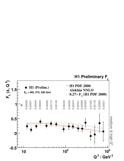
Figure 2: The H1 experimental results for the longitudinal proton structure function, $F_{L}(x,Q^{2})$, compared with the prediction of $F_{L}(x,Q^{2})=0.27\times F_{2}(x,Q^{2})$ from transverse-size enhancement of transversely relative to longitudinally polarized $(q\bar{q})^{J=1}$ states.

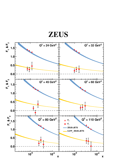
Figure 3: The ZEUS experimental results for the longitudinal proton structure function, $F_{L}(x,Q^{2})$, compared with the prediction of $F_{L}(x,Q^{2})=0.27\times F_{2}(x,Q^{2})$ from transverse-size enhancement of transversely relative to longitudinally polarized $(q\bar{q})^{J=1}$ states.

2.4 Discussion on the Representations of the CDP in Sections 2.1 and 2.2

.

The CDP of DIS at low x is based on a life-time argument concerning massive hadronic fluctuations of the photon. The argument is identical to the one put forward in the space-time interpretation [2, 18] of generalized vector dominance in the early 1970ies. The life-time in the rest frame of the nucleon of a hadronic fluctuation of mass $M_{q\bar{q}}$, given by the covariant expression [19]

$$\frac{1}{\Delta E}=\frac{1}{x+\frac{M^{2}_{q\bar{q}}}{W^{2}}}\frac{1}{M_{p}}\gg\frac{1}{M_{p}},$$ (2.60)

becomes large in comparison with the inverse of the proton mass, $M_{p}$, provided $x\cong Q^{2}/W^{2}\ll 1$ and the c.m. energy, $W$, is sufficiently large. The $\gamma^{*}p$ interaction with the nucleon at low x, accordingly, proceeds via the interaction of hadronic $q\bar{q}$ fluctuations of timelike four-momentum squared identical to $M^{2}_{(q\bar{q})}$. More definitely, the integration over the dipole cross section $\sigma_{(q\bar{q})p}(r_{\bot},z(1-z),W^{2})$ in transverse position space in (2.1) describes the interaction of a continuum of massive $q\bar{q}$ states. The dipole cross section depends on $W^{2}$ , just as any other purely hadronic interaction cross section. In particular, the dipole cross section does not depend on the virtuality, $Q^{2}$, of the photon, and consequently, it does not depend on $x$.

The dipole cross section in (2.1) does not refer to a definite spin $J$ of the massive $q\bar{q}$ continuum states. The interaction with the nucleon, nevertheless, proceeds via the spin $J=1$ projection of the dipole cross section $\sigma_{(q\bar{q})p}(r_{\bot},z(1-z),W^{2})$, compare the discussion in Section 2.2, in particular the relations (2.39) and (2.2).

The $W$ dependence of the dipole cross section explicitly, via $\tilde{\sigma}(\vec{l}^{~{}2}_{\bot},z(1-z),W^{2})$ in (2.16) and $\bar{\sigma}_{(q\bar{q})^{J=1}_{L}p}(\vec{l}^{~{}\prime 2}_{\bot},W^{2})$ in (2.51) with (2.56), enters the large-$Q^{2}$ approximation of the photoabsorption cross section. Inserting (2.16) and (2.51) into the proton structure function,

$$F_{2}(x,Q^{2}) = \frac{Q^{4}(1-x)}{4\pi^{2}\alpha(Q^{2}+(2M_{p}x)^{2})}\left(\sigma_{\gamma^{*}_{L}p}(W^{2},Q^{2})+\sigma_{\gamma^{*}_{T}p}(W^{2},Q^{2})\right)\cong$$ (2.61)

$$\cong \frac{Q^{2}}{4\pi^{2}\alpha}\left(\sigma_{\gamma^{*}_{L}p}(W^{2},Q^{2})+\sigma_{\gamma^{*}_{T}p}(W^{2},Q^{2})\right)$$

one finds

$$F_{2}(x,Q^{2})=\frac{\sum_{q}Q^{2}_{q}}{4\pi^{2}}\int dz\int d\vec{l}^{~{}2}_{\bot}\vec{l}^{~{}2}_{\bot}\tilde{\sigma}(\vec{l}^{~{}2}_{\bot},z(1-z),W^{2})(1+2\rho),$$ (2.62)

and

$$F_{2}(x,Q^{2})=\frac{\sum_{q}Q^{2}_{q}}{4\pi^{2}}\frac{1}{6}\int d\vec{l}^{~{}\prime 2}_{\bot}\vec{l}^{~{}\prime 2}_{\bot}\bar{\sigma}_{(q\bar{q})^{J=1}_{L}p}(\vec{l}^{~{}\prime 2}_{\bot},W^{2})\left(1+2\rho\right),$$ (2.63)

where $\rho$ for $Q^{2}$ sufficiently large is given in (2.56). According to the right-hand sides in (2.62) and (2.63), the structure function only depends on $W^{2}=Q^{2}/x$ in the color-transparency region of sufficiently large $Q^{2}$ and sufficiently small $x<0.1$.

The $W^{2}$ dependence in (2.62) and (2.63) can be empirically tested by plotting the experimental data for the proton structure function $F_{2}(x\cong Q^{2}/W^{2},Q^{2})$ as a function of $1/W^{2}$.

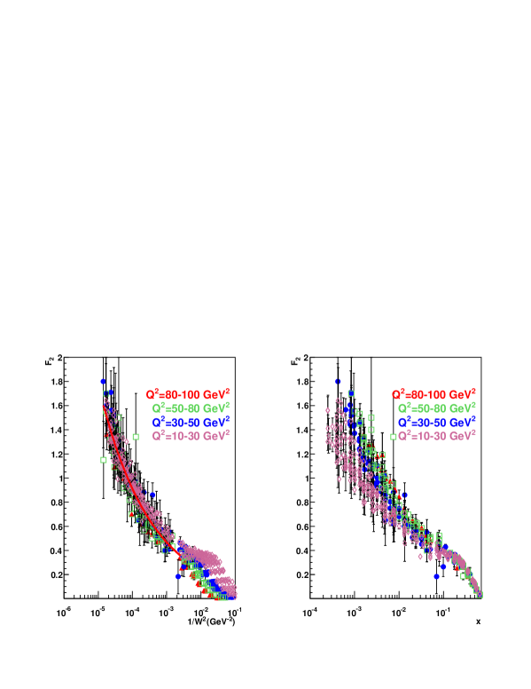
Fig.4a                                     Fig.4b

Figure 4: In fig.4a we show the experimental data for $F_{2}(x\cong Q^{2}/W^{2},Q^{2})$ as a function of $1/W^{2}$, and in fig.4b, for comparison, as a function of $x$. The theoretical prediction based on (2.124) and (2.125) is also shown in fig.4a.

In fig. 4a, we show the experimental data from HERA for $Q^{2}$ in the large range of $10GeV^{2}\leq Q^{2}\leq 100GeV^{2}$ as a function of $1/W^{2}$. In the relevant range of $x\cong Q^{2}/W^{2}<0.1$, approximately corresponding to $1/W^{2}\leq 10^{-3}$, the experimental data show indeed a tendency to lie on a single line, quite in contrast to the range of $1/W^{2}\geq 10^{-3}$. The opposite tendency of the experimental data, approximate clustering around a single line for $x\geq 0.1$, but stronger deviations from a single line at $x\leq 0.1$ is seen in fig. 4b, where the same experimental data for $F_{2}(x,Q^{2})$ are plotted in the usual manner as a function of Bjorken $x$. The replacement of $W^{2}$ by $W^{2}\simeq Q^{2}/x$, when passing from fig. 4a to fig. 4b now yields the well-known increased violation of Bjorken scaling in the diffraction region of $x<0.1$. Compare Section 2.7 for a discussion of the theoretical prediction shown in fig.4a.

We summarize: DIS at low $x$ proceeds via the imaginary part of the forward scattering amplitude of a continuum of massive $(q\bar{q})^{J=1}_{L,T}$ states. The interaction of the $q\bar{q}$ color dipole with the gluon field of the proton, by gauge invariance, fulfills (2.2) and (2.44), implying color transparency, (2.3) and (2.46). For $Q^{2}$ sufficiently large (with $x\cong Q^{2}/W^{2}\ll 0.1$ sufficiently small), the structure function $F_{2}(x,Q^{2})$ only depends on the single variable $W$. No details of perturbative QCD beyond the gauge-invariant color-dipole interaction are needed to deduce the CDP of Sections 2.1 and 2.2, and this (approximate) dependence of $F_{2}(x,Q^{2})$ on the single variable $W^{2}$ for $Q^{2}$ sufficiently large. In particular, no reference to details of the perturbative gluon density of the proton is needed. In this connection, also compare the derivation of the CDP in ref. [6] as well as the formally much more complete and elaborate derivation in ref. [15].

By starting from the $\vec{l}_{\bot}$-factorization approach, under certain assumptions, one may introduce a CDP-like representation [5, 20] for the photoabsorption cross section containing $x$ instead of $W^{2}$ in the dipole cross section in (2.1). Such a representation does not factorize the $Q^{2}$ dependence inherently connected with the photon wave function and the $W$ dependence that governs the $(q\bar{q})p$ dipole interaction. As a consequence, the CDP-like representation is ill-suited to represent the transition from large $Q^{2}$ to small $Q^{2}$ including the solely $W$-dependent cross section of $Q^{2}=0$ photoproduction. Examining and understanding this transition to low $x\cong Q^{2}/W^{2}$ photoabsorption, however, is the main aim and also the essential achievement of the CDP-representation of DIS at low $x$.

2.5 Low-x Scaling

A model-independent analysis of the experimental data on DIS from HERA has revealed [11, 21] that the photoabsorption cross section, $\sigma_{\gamma^{*}p}(W^{2},Q^{2})$, at low $x$ is a function of the low-x scaling variable

$$\eta(W^{2},Q^{2})=\frac{Q^{2}+m^{2}_{0}}{\Lambda^{2}_{sat}(W^{2})},$$ (2.64)

i.e. a function of the single variable $\eta(W^{2},Q^{2})$,

$$\sigma_{\gamma^{*}p}(W^{2},Q^{2})=\sigma_{\gamma^{*}p}\left(\eta(W^{2},Q^{2})\right).$$ (2.65)

In (2.64) and (2.65), the “saturation scale”, $\Lambda^{2}_{sat}(W^{2})$, empirically increases as $\Lambda^{2}_{sat}(W^{2})\sim(W^{2})^{C_{2}}$, with $C_{2}\cong 0.27$ and $m^{2}_{0}\cong 0.15GeV^{2}$ [11, 21]. The empirical analysis of the experimental data showed that $\sigma_{\gamma^{*}p}\left(\eta(W^{2},Q^{2})\right)$ for large $\eta(W^{2},Q^{2})\gg 1$ is inversely proportional to $\eta(W^{2},Q^{2})$,

$$\sigma_{\gamma^{*}p}(W^{2},Q^{2})\sim\sigma^{(\infty)}(W^{2})\frac{1}{\eta(W^{2},Q^{2})},$$ (2.66)

while for small values of $\eta(W^{2},Q^{2})\ll 1$, the dependence on $\eta(W^{2},Q^{2})$ is logarithmic,

$$\sigma_{\gamma^{*}p}(W^{2},Q^{2})\sim\sigma^{(\infty)}(W^{2})\ln\frac{1}{\eta(W^{2},Q^{2})},~{}~{}(\eta(W^{2},Q^{2})\ll 1).$$ (2.67)

In (2.66) and (2.67) the cross section $\sigma^{(\infty)}(W^{2})$ empirically was found to be of hadronic size and approximately constant, $\sigma^{(\infty)}(W^{2})\simeq const.$, as a function of the energy $W$.

In the present Section 2.5, we will show that not only the existence of the scaling behavior (2.65), but also the observed functional dependence of the cross section, as $1/\eta(W^{2},Q^{2})$ for large $\eta(W^{2},Q^{2})$, and as $\ln(1/\eta(W^{2},Q^{2}))$ for small $\eta(W^{2},Q^{2})$, in (2.66) and (2.67), respectively, is a general and direct consequence of the color-dipole nature of the interaction of the hadronic fluctuations of the photon with the color field in the nucleon. No specific parameterization of the color-dipole-proton cross section, $\sigma_{(q\bar{q})p}(r_{\bot},z(1-z),W^{2})$, must be introduced to deduce the empirically observed functional dependence in (2.66) and (2.67).

The ensuing analysis will be based on the representation of the photoabsorption cross section in Section 2.2 in terms of the scattering of $(q\bar{q})^{J=1}_{L,T}$ states on the proton. Compare (2.39) in particular, as well as the longitudinal and transverse dipole cross sections given by (2.44). The representation (2.44) of the dipole cross section, as a consequence of (2.2), is solely based on the gauge-invariant coupling of the color-dipole state to the gluon field in the nucleon.

Upon angular integration, (2.44) becomes

$$\sigma_{(q\bar{q})^{J=1}_{L,T}p}(r^{\prime}_{\bot},W^{2}) =\pi\int d\vec{l}^{~{}\prime 2}_{\bot}\bar{\sigma}_{(q\bar{q})^{J=1}_{L,T}p}(\vec{l}^{~{}\prime 2}_{\bot},W^{2}).$$ (2.68)

$$\cdot\left(1-\frac{\int d\vec{l}^{~{}\prime 2}_{\bot}\bar{\sigma}_{(q\bar{q})^{J=1}_{L,T}p}(\vec{l}^{~{}\prime 2}_{\bot},W^{2})J_{0}(l^{\prime}_{\bot}r^{\prime}_{\bot})}{\int d\vec{l}^{~{}\prime 2}_{\bot}\bar{\sigma}_{(q\bar{q})^{J=1}_{L,T}p}(\vec{l}^{~{}\prime 2}_{\bot},W^{2})}\right),$$

where $r^{\prime}_{\bot}\equiv\sqrt{\vec{r}^{~{}\prime 2}_{\bot}}$ and $J_{0}(l^{\prime}_{\bot}r^{\prime}_{\bot})$ denotes the Bessel function of order zero. We assume that the integrals in (2.68) do exist and are determined by the integrands in a restricted range of $\vec{l}^{~{}\prime 2}_{\bot}<\vec{l}^{~{}\prime 2}_{\bot~{}Max}\equiv l^{\prime 2}_{\bot~{}Max}(W^{2})$, where $\bar{\sigma}_{(q\bar{q})^{J=1}_{L,T}p}(\vec{l}^{~{}\prime 2}_{\bot},W^{2})$ is appreciably different from zero. The resulting dipole cross section (2.68), for any fixed value of $r^{\prime}_{\bot}$, strongly depends on the variation of the phase, $l^{\prime}_{\bot}r^{\prime}_{\bot}$, in (2.44) and (2.68) as a function of $l^{\prime}_{\bot}<l^{\prime}_{\bot~{}Max}(W^{2})$.

Indeed, if for a given value of $r^{\prime}_{\bot}$ the phase $l^{\prime}_{\bot}r^{\prime}_{\bot}$ in the relevant range of $l^{\prime}_{\bot}<l^{\prime}_{\bot~{}Max}(W^{2})$ is always smaller than unity, i.e.

$$0<l^{\prime}_{\bot}r^{\prime}_{\bot}<l^{\prime}_{\bot~{}Max}(W^{2})r^{\prime}_{\bot}\ll 1,$$ (2.69)

the second term in the bracket of (2.68) essentially cancels the first one, since

$$J_{0}(l^{\prime}_{\bot}r^{\prime}_{\bot})\cong 1-\frac{1}{4}(l^{\prime}_{\bot}r^{\prime}_{\bot})^{2}+\frac{1}{4^{3}}(l^{\prime}_{\bot}r^{\prime}_{\bot})^{4}+\cdots.$$ (2.70)

Substitution of (2.70) into (2.68) implies the proportionality of the dipole cross section to $r^{\prime 2}_{\bot}$ already given in (2.46). Combining (2.46) with (2.49) and (2.56), we find

$$\sigma_{(q\bar{q})^{J=1}_{L,T}p}(r^{\prime 2}_{\bot},W^{2})=$$ (2.71)

$$=\frac{1}{4}\pi r^{\prime 2}_{\bot}\int d\vec{l}^{~{}\prime 2}_{\bot}\vec{l}^{~{}\prime 2}_{\bot}\bar{\sigma}_{(q\bar{q})^{J=1}_{L}p}(\vec{l}^{~{}\prime 2}_{\bot},W^{2})\left\{\matrix{1,\cr\rho,}\right.\left(r^{\prime 2}_{\bot}\ll\frac{1}{l^{\prime 2}_{\bot~{}Max}(W^{2})}\right).$$

In the limiting case of

$$l^{\prime}_{\bot Max}(W^{2})r^{\prime}_{\bot}\gg 1,$$ (2.72)

alternative to (2.69), the rapid oscillation of the Bessel function under variation of $0<l^{\prime}_{\bot}<l^{\prime}_{\bot~{}Max}(W)$ at fixed $r^{\prime}_{\bot}$ implies a vanishing contribution of the second term in (2.68). The dipole cross section (2.68) in this limit is not proportional to the dipole size $\vec{r}_{\bot}^{~{}\prime 2}$, but, in distinction from (2.71), becomes identical to the $\vec{r}^{~{}\prime 2}_{\bot}$-independent limit $\sigma^{(\infty)}_{L,T}(W^{2})$ of normal hadronic size,

$$\sigma_{(q\bar{q})^{J=1}_{L,T}p}(r_{\bot}^{~{}\prime 2},W^{2}) \cong\pi\int d\vec{l}^{~{}\prime 2}_{\bot}\bar{\sigma}_{(q\bar{q})^{J=1}_{L,T}p}(\vec{l}^{~{}\prime 2}_{\bot},W^{2})\equiv\sigma^{(\infty)}_{L,T}(W^{2}),$$ (2.73)

$$\left(r^{\prime 2}_{\bot}\gg\frac{1}{l^{\prime 2}_{\bot~{}Max}(W^{2})}\right).$$

We note that the $r_{\bot}^{\prime}$-independent limit on the right-hand side in (2.73) obtained at any fixed value of $r_{\bot}^{\prime}$ for $l^{\prime 2}_{\bot\max}(W^{2})\rightarrow\infty$ coincides with the limit of $r^{\prime}_{\bot}\rightarrow\infty$ at fixed energy, $W$, or fixed $\vec{l}^{~{}\prime 2}_{\bot\max}(W^{2})$. A small $q\bar{q}$ dipole at infinite energy yields the same cross section as a sufficiently large dipole at finite energy $W$.

The gauge-invariant color-dipole interaction with the gluon thus implies the emergence of two scales, the helicity-dependent integral over
$\bar{\sigma}_{(q\bar{q})^{J=1}_{L,T}p}(\vec{l}^{~{}\prime 2}_{\bot},W^{2})$ in (2.73) and the first moment of $\bar{\sigma}_{(q\bar{q})^{J=1}_{L}}(l^{\prime 2}_{\bot},W^{2})$ in (2.71), which determine the dipole cross section for relatively large $r^{\prime 2}_{\bot}$ and relatively small $r^{\prime 2}_{\bot}$, respectively. Whether (2.73) or (2.71) is relevant for a chosen value of $r^{\prime}_{\bot}$ depends on the value of $l^{\prime 2}_{\bot~{}Max}(W^{2})$ that in turn depends on the $W$-dependence of the $(q\bar{q})^{J=1}_{L,T}p$ dipole cross section, $\bar{\sigma}_{(q\bar{q})^{J=1}_{L,T}p}(\vec{l}^{~{}\prime 2}_{\bot},W^{2})$.

It is appropriate to introduce and use the normalized distribution in $\vec{l}^{~{}\prime 2}_{\bot}$,

$$\Lambda^{2}_{sat}(W^{2}) \equiv \frac{\int d\vec{l}^{~{}\prime 2}_{\bot}\vec{l}^{~{}\prime 2}_{\bot}\bar{\sigma}_{(q\bar{q})^{J=1}_{L}p}(\vec{l}^{~{}\prime 2}_{\bot},W^{2})}{\int d\vec{l}^{~{}\prime 2}_{\bot}\bar{\sigma}_{(q\bar{q})^{J=1}_{L}p}(\vec{l}^{~{}\prime 2}_{\bot},W^{2})}=$$ (2.74)

$$= \frac{1}{\sigma^{(\infty)}_{L}(W^{2})}\pi\cdot\int d\vec{l}^{~{}\prime 2}_{\bot}\vec{l}^{~{}\prime 2}_{\bot}\bar{\sigma}_{(q\bar{q})^{J=1}_{L}p}(\vec{l}^{~{}\prime 2}_{\bot},W^{2}),$$

as the second scale besides $\sigma^{(\infty)}_{L,T}(W^{2})$ from (2.73). The $r^{\prime 2}_{\bot}\to 0$ limit in (2.71) then becomes

$$\sigma_{(q\bar{q})^{J=1}_{L,T}p}(r^{\prime 2}_{\bot},W^{2})=\frac{1}{4}r^{\prime 2}_{\bot}\sigma^{(\infty)}_{L}(W^{2})\Lambda^{2}_{sat}(W^{2})\left\{\matrix{1,\cr\rho,}\right.~{}\left(r^{\prime 2}_{\bot}\ll\frac{1}{l^{\prime 2}_{\bot~{}Max}(W^{2})}\right).$$ (2.75)

The cross section $\sigma^{(\infty)}_{L,T}(W^{2})$, as a consequence of the color-dipole interaction in (2.2) and (2.44), according to (2.73) and (2.75), is of relevance for both, the $r^{\prime 2}_{\bot}\to\infty$ as well as the $r^{\prime 2}_{\bot}\to 0$ behavior of the dipole cross section.

Before returning to the photoabsorption cross section, we add a further comment on the dipole cross section (2.68) and its important limits in (2.71) (or, equivalently, in (2.75)) and in (2.73). The dependence of the dipole cross section (2.68) on $r^{\prime}_{\bot}$ is determined by the destructive interference originating from the (negative) second term in the bracket in (2.68). At any fixed value of $r^{\prime}_{\bot}$, for sufficiently high energy, i.e. with increasingly greater values of $\vec{l}^{~{}\prime 2}_{\bot~{}Max}(W^{2})$, the vanishing of this term, due to strong oscillations of the integrand leads to the $\vec{r}^{~{}\prime}_{\bot}$-independent limit of a cross section of hadronic size in (2.73). With increasing energy a transition occurs from the region of color transparency (2.71), where the cross section is proportional to the dipole size, $\vec{r}^{~{}\prime 2}_{\bot}$, to the saturation regime (2.73) characterized by a cross section that is independent of the dipole size, $\vec{r}^{~{}\prime 2}_{\bot}$; the interaction of a colorless $q\bar{q}$ dipole is in the saturation regime replaced by the interaction of a colored quark and a colored antiquark thus producing a cross section of hadronic size. Both, color transparency, as well as the transition to the hadronlike saturation behavior, are recognized as a genuine consequence of the gauge-invariant color-dipole interaction (2.1). It is a misconception to associate the saturation regime with an increased density in a small-size region of the proton: in the high-energy limit of (2.73) the cross section is not proportional to the dipole size, and therefore it cannot be interpreted as the product of a (small) dipole size with a high-gluon-density region.

We turn to the photoabsorption cross section in (2.33). The integration over $d^{2}\vec{r}^{~{}\prime}_{\bot}$ in (2.33) at fixed $Q^{2}$ is dominated by

$$\vec{r}^{~{}\prime 2}_{\bot}\equiv r^{\prime 2}_{\bot}\leq\frac{1}{Q^{2}}.$$ (2.76)

Compare (2.7) and (2.8). The resulting photoabsorption cross section for fixed $Q^{2}$ then depends on whether the limiting case of either (2.71) (or equivalently (2.75)) or of (2.73) is relevant for $r^{\prime 2}_{\bot}\leq 1/Q^{2}$.

For the case of

$$r^{\prime 2}_{\bot}<\frac{1}{Q^{2}}\ll\frac{1}{l^{\prime 2}_{\bot~{}Max}(W^{2})},$$ (2.77)

the $r^{\prime 2}_{\bot}\to 0$ expression in (2.75) is relevant. This region of relatively large $Q^{2}$ was treated in Section 2.2. Compare (2.46) and (2.47). Introducing $\Lambda^{2}_{sat}(W^{2})$ from (2.74) and (2.75) on the right-hand side of (2.51), with $\rho_{W}=\rho$ from (2.56), we find

$$\sigma_{\gamma^{*}_{L,T}p}(W^{2},Q^{2})=\frac{\alpha}{\pi}\sum_{q}Q^{2}_{q}\frac{1}{6}\sigma^{(\infty)}_{L}(W^{2})\frac{\Lambda^{2}_{{\rm sat}}(W^{2})}{Q^{2}}\left\{\matrix{1,\cr 2\rho.}\right.$$ (2.78)

The total photoabsorption cross section is given by

$$\sigma_{\gamma^{*}p}(W^{2},Q^{2}) = \sigma_{\gamma^{*}_{L}p}(W^{2},Q^{2})+\sigma_{\gamma^{*}_{T}p}(W^{2},Q^{2})$$ (2.79)

$$= \frac{\alpha}{\pi}\sum_{q}Q^{2}_{q}(1+2\rho)\frac{1}{6}\sigma^{(\infty)}_{L}(W^{2})\frac{\Lambda^{2}_{sat}(W^{2})}{Q^{2}}.$$

Unitarity requires the hadronic dipole cross section, $\sigma^{\infty}_{L,T}(W^{2})$, from (2.73) to only weakly depend on $W^{2}$,

$$\sigma^{(\infty)}_{L,T}(W^{2})\cong~{}{\rm const.}$$ (2.80)

Moreover, motivated by quark confinement and/or quark-hadron duality [23], the divergence of $r^{\prime 2}_{\bot}\to\infty$ for $Q^{2}\to 0$ in (2.76) must be replaced by

$$r^{\prime 2}_{\bot}<\frac{1}{Q^{2}+m^{2}_{0}},$$ (2.81)

where $m^{2}_{0}$ actually depends on the quark flavor. For light quarks, $m^{2}_{0}\mathrel{\raise 1.29167pt\hbox{$<$\kern-7.5pt\lower 4.30554pt\hbox{$\sim$}}}m^{2}_{\rho}$, where $m_{\rho}$ is the $\rho^{0}$ meson mass, is relevant. Replacing $Q^{2}\to Q^{2}+m^{2}_{0}$ in (2.79), and identifying the resulting (inverse) ratio with the empirical parameter $\eta(W^{2},Q^{2})$ in (2.64), we have

$$\sigma_{\gamma^{*}p}(W^{2},Q^{2})=\frac{\alpha}{\pi}\sum_{q}Q^{2}_{q}(1+2\rho)\frac{1}{6}\sigma^{(\infty)}_{L}(W^{2})\frac{1}{\eta(W^{2},Q^{2})},~{}~{}~{}(\eta(W^{2},Q^{2})\gg 1),$$ (2.82)

where $\eta(W^{2},Q^{2})\gg 1$ as a consequence of (2.77) and (2.74). With (2.80), this is the empirically established scaling behavior (2.66).

We turn to the case of

$$\frac{1}{l^{\prime 2}_{\bot~{}Max}(W^{2})}\ll\frac{1}{Q^{2}},$$ (2.83)

alternative to (2.77), and relevant in particular for large values of the energy $W$ and relatively small values of $Q^{2}$. In this case of (2.83), within the integration domain of $r^{\prime 2}_{\bot}<1/Q^{2}$ from (2.76), we have to discriminate two different regions. For

$$r^{\prime 2}_{\bot}<\frac{1}{\vec{l}^{~{}\prime 2}_{\bot~{}Max}(W^{2})}\ll\frac{1}{Q^{2}},$$ (2.84)

we have color transparency (2.75). In distinction from (2.77), color transparency only holds in a small restricted domain of the full integration interval $r^{\prime 2}_{\bot}<1/Q^{2}$. For the remaining integration domain,

$$\frac{1}{\vec{l}^{~{}\prime 2}_{\bot~{}Max}(W^{2})}<r^{\prime 2}_{\bot}<\frac{1}{Q^{2}},$$ (2.85)

the $r^{\prime}_{\bot}$-independent dipole cross section (2.73) becomes relevant.

It is useful to split the integration domain into the sum of two different ones. Noting that according to the definition (2.74),

$$\Lambda^{2}_{sat}(W^{2})\mathrel{\raise 1.29167pt\hbox{$<$\kern-7.5pt\lower 4.30554pt\hbox{$\sim$}}}l^{\prime 2}_{\bot~{}Max}(W^{2}),$$ (2.86)

we use $\Lambda^{2}_{sat}(W^{2})$ as the splitting parameter of the integral over $dr^{\prime 2}_{\bot}$. The photoabsorption cross section (2.39) then becomes

$$\sigma_{\gamma^{*}_{L,T}p}(W^{2},Q^{2}) = \frac{\alpha}{\pi}\sum_{q}Q^{2}_{q}Q^{2}\left(\int^{\frac{1}{\Lambda^{2}_{sat}(W^{2})}}_{0}dr^{\prime 2}_{\bot}+\int^{\frac{1}{Q^{2}}}_{\frac{1}{\Lambda^{2}_{sat}(W^{2})}}dr^{\prime 2}_{\bot}\right)\cdot$$ (2.87)

$$\cdot K^{2}_{0,1}(r^{\prime}_{\bot}Q)\sigma_{(q\bar{q})^{J=1}_{L,T}p}(r^{\prime 2}_{\bot},W^{2}).$$

The main contribution to the photoabsorption cross section is due to the second term on the right-hand side in (2.87). The first term will subsequently be shown to be negligible compared with the second one. Only taking into account the second term, upon introducing the $r^{\prime}_{\bot}$-independent dipole cross section from (2.73), we find

$$\sigma_{\gamma^{*}_{L,T}p}(W^{2},Q^{2})=\frac{2\alpha}{\pi}\sum Q^{2}_{q}Q^{2}\left\{\matrix{\sigma^{(\infty)}_{L}(W^{2})\int^{\frac{1}{Q}}_{\frac{1}{\Lambda_{sat}(W^{2})}}dr^{\prime}_{\bot}r^{\prime}_{\bot}K^{2}_{0}(r^{\prime}_{\bot}Q),\cr\sigma^{(\infty)}_{T}(W^{2})\int^{\frac{1}{Q}}_{\frac{1}{\Lambda_{sat}(W^{2})}}dr^{\prime}_{\bot}r^{\prime}_{\bot}K^{2}_{1}(r^{\prime}_{\bot}Q).}\right.$$ (2.88)

The cross section in the high-energy limit, (2.88), as a consequence of the factorization of the dipole cross section (2.73), is directly given by an integral over the photon wave function, compare e.g. (2.88) with the general expression in (2.39).

In the integration domain (2.85) of $r^{\prime}_{\bot}Q<1$, relevant in (2.87) and (2.88), upon introducing $y=r^{\prime}_{\bot}Q$, we can approximate $K^{2}_{0,1}(r^{\prime}_{\bot}Q)=K^{2}_{0,1}(y)$ by

$$K^{2}_{0}(y) \simeq \ln^{2}y,$$

$$K^{2}_{1}(y) \simeq \frac{1}{y^{2}},~{}~{}~{}~{}~{}~{}(y<1).$$ (2.89)

We find

$$\sigma_{\gamma^{*}_{L,T}p}(W^{2},Q^{2})=\frac{2\alpha}{\pi}\sum Q^{2}_{q}\left\{\matrix{\frac{1}{4}\sigma^{(\infty)}_{L}(W^{2}),~{}~{}~{}~{}~{}~{}~{}~{}~{}~{}~{}~{}~{}~{}\cr\frac{1}{2}\sigma_{T}^{(\infty)}(W^{2})\ln\frac{\Lambda^{2}_{sat}(W^{2})}{Q^{2}}.}\right.$$ (2.90)

The longitudinal cross section becomes small in this limit of very high energy $W$ and comparatively small values of $Q^{2}$. According to (2.90), the longitudinal cross section may be neglected, and the total cross section is given by

$$\sigma_{\gamma^{*}p}(W^{2},Q^{2})=\frac{\alpha}{\pi}\sum Q^{2}_{q}\sigma^{(\infty)}_{T}(W^{2})\ln\frac{\Lambda^{2}_{sat}(W^{2})}{Q^{2}}.$$ (2.91)

With the replacement of $Q^{2}\to Q^{2}+m^{2}_{0}$, compare (2.81), and upon introducing $\eta(W^{2},Q^{2})$ from (2.64), we indeed have derived the empirically observed logarithmic dependence,

$$\sigma_{\gamma^{*}p}(W^{2},Q^{2})=\frac{\alpha}{\pi}\sum Q^{2}_{q}\sigma^{(\infty)}_{T}(W^{2})\ln\frac{1}{\eta(W^{2},Q^{2})}~{},~{}(\eta(W^{2},Q^{2})\ll 1),$$ (2.92)

where $\sigma_{T}^{(\infty)}(W^{2})\cong~{}{\rm const}$, compare (2.80).

Combining (2.78) and (2.90), the ratio $R$ of the longitudinal and the transverse parts of the photoabsorption cross section is given by

$$R(W^{2},Q^{2})=\frac{1}{2}\left\{\matrix{\frac{\sigma_{L}^{(\infty)}(W^{2})}{\sigma_{T}^{(\infty)}(W^{2})}\frac{1}{\ln\frac{1}{\eta(W^{2},Q^{2})}},(\eta(W^{2},Q^{2})\ll 1),\cr\frac{1}{\rho},~{}~{}~{}~{}~{}~{}~{}~{}~{}~{}~{}~{}~{}~{}~{}~{}~{}~{}~{}(\eta(W^{2},Q^{2})\gg 1).}\right.$$ (2.93)

In the limit of $\eta(W^{2},Q^{2})\ll 1$, i.e. for $W^{2}\to\infty$ at fixed $Q^{2}$, the longitudinal part of the photoabsorption cross section becomes vanishingly small compared with the transverse part. In the limit of $\eta(W^{2},Q^{2})\gg 1$, we have $\rho=4/3$ from transverse-size enhancement, while $\rho=1$ under the ad hoc assumption of helicity independence.

We finally have to convince ourselves that the first term in (2.87) can be neglected relative to the second one. Inserting (2.75) into (2.39), the contribution of the first term becomes

$$\sigma^{(I)}_{\gamma^{*}_{L,T}p}(W^{2},Q^{2})=\frac{\alpha}{\pi}\sum_{q}Q^{2}_{q}\frac{1}{2}\sigma_{L}^{(\infty)}(W^{2})\frac{\Lambda^{2}_{sat}(W^{2})}{Q^{2}}\left\{\matrix{\int^{\frac{Q}{\Lambda_{sat}(W^{2})}}_{0}dyy^{3}K^{2}_{0}(y),\cr\rho\int^{\frac{Q}{\Lambda_{sat}(W^{2})}}_{0}dyy^{3}K^{2}_{1}(y).}\right.$$ (2.94)

Evaluation of the integrals upon inserting (2.89) yields

$$\sigma^{(I)}_{\gamma^{*}p}(W^{2},Q^{2}) = \frac{\alpha\sum_{q}Q^{2}_{q}}{\pi}\frac{1}{4}\sigma_{L}^{(\infty)}(W^{2})\left(\frac{1}{2}\frac{Q^{2}}{\Lambda^{2}_{sat}(W^{2})}\ln^{2}\frac{Q^{2}}{\Lambda^{2}_{sat}(W^{2})}+\rho\right)$$ (2.95)

$$\cong \frac{\alpha\sum Q^{2}_{q}}{\pi}\frac{1}{4}\sigma_{L}^{(\infty)}(W^{2})\rho,~{}~{}~{}~{}~{}(\Lambda^{2}_{sat}(W^{2})\gg Q^{2}).$$

Since (2.91) is enhanced by $\ln(\Lambda^{2}_{sat}(W^{2})/Q^{2})$, we can neglect (2.95) for sufficiently large $\Lambda^{2}_{sat}(W^{2})$.

The resulting cross sections (2.82) and (2.92) establish the empirically observed low-x scaling behavior as a consequence of the interaction of the $q\bar{q}$-fluctuations of the (real or virtual) photon as color-dipole states. Low-$x$ scaling is recognized as a genuine consequence of the CDP in the formulation given in (2.39) and (2.44) that is based on (2.1) and (2.2). “Saturation” i.e. the slow logarithmic increase as $\ln\Lambda^{2}_{sat}(W^{2})$ in (2.92), is not based on a specific model assumption. It occurs as a consequence of the transition of the $(q\bar{q})p$ interaction from the color-transparency region to the hadronic one. This transition occurs for any given $Q^{2}$, or any fixed dipole size, provided the energy is sufficiently high such that the $q\bar{q}$ state does not interact as a colorless dipole, but rather as a system of two colored quarks.

2.6 The photoproduction limit for $W^{2}\to\infty$ at fixed $Q^{2}>0$.

In Section 2.5, we found that the CDP from (2.1) and (2.2) implies that the photoabsorption cross section at low $x\cong Q^{2}/W^{2}\ll 1$ depends on the single scaling variable $\eta(W^{2},Q^{2})$ from (2.64) and (2.74). Moreover, the dependence of $\sigma_{\gamma^{*}_{L,T}p}(\eta(W^{2},Q^{2}))$, for small and large values of $\eta(W^{2},Q^{2})$ was found to be uniquely determined without adopting a specific parameterization for the dipole cross section, compare (2.92) and (2.82),

$$\sigma_{\gamma^{*}p}(W^{2},Q^{2}) = \sigma_{\gamma^{*}p}(\eta(W^{2},Q^{2}))=$$

$$= \frac{\alpha}{\pi}\sum_{q}Q^{2}_{q}\left\{\matrix{\sigma^{(\infty)}_{T}(W^{2})\ln\frac{1}{\eta(W^{2},Q^{2})},~{}~{}~{}(\eta(W^{2},Q^{2})\ll 1),\cr\frac{1}{6}(1+2\rho)\sigma_{L}^{(\infty)}(W^{2})\frac{1}{\eta(W^{2},Q^{2})},~{}~{}~{}(\eta(W^{2},Q^{2})\gg 1).}\right.$$

where unitarity restricts $\sigma_{L,T}^{(\infty)}(W^{2})$ to being at most weakly dependent on $W$. In this Section 2.6, we present a more detailed discussion of the important $\eta(W^{2},Q^{2})\to 0$ limit of $W^{2}\to\infty$ at fixed values of $Q^{2}$.

We explicitly assume $\Lambda^{2}_{sat}(W^{2})$ to increase with the energy, $W$. There are convincing theoretical arguments for this assumption, independent of the analysis of the experimental data that was referred to in the discussion related to (2.64) to (2.67).

Note that the absorption of a gluon of transverse momentum $\vec{l}_{\bot}$ by a $q\bar{q}$ fluctuation leads to “diagonal” as well as “off-diagonal” transitions with respect to the mass, $M_{q\bar{q}}$, of the $q\bar{q}$ fluctuations,

$$(q\bar{q})_{M_{q\bar{q}}}\to\left\{\matrix{(q\bar{q})_{M_{q\bar{q}}},~{}~{}~{}~{}~{}~{}~{}{\rm``diagonal")},\cr(q\bar{q})_{M^{\prime}_{q\bar{q}}\not=M_{q\bar{q}}},~{}~{}~{}~{}~{}~{}~{}~{}{\rm(``off-diagonal")}.}\right.$$ (2.97)

The mass difference in the second line of (2.97) is proportional to $\vec{l}^{~{}\prime 2}_{\bot}=\vec{l}^{~{}2}_{\bot}/z(1-z)$, or to $\Lambda^{2}_{sat}(W^{2})$ from (2.74), on the average,

$$\Delta M^{2}_{q\bar{q}}\equiv M^{\prime 2}_{q\bar{q}}-M^{2}_{q\bar{q}}\sim\Lambda^{2}_{sat}(W^{2}).$$ (2.98)

This connection excludes $\Lambda^{2}_{sat}(W^{2})=const.$ unless one is willing to postulate the mass difference between incoming and outgoing $q\bar{q}$ states in hadronic diffraction to be equal to a fixed value that is $W$-independent, even for $W\to\infty$. Constancy, $\Lambda^{2}_{sat}(W^{2})={\rm const.}$, would imply a $W$-dependence of the photoabsorption cross section (2.6) that is exclusively determined by the factorized cross section $\sigma_{L,T}^{(\infty)}(W^{2})$ from (2.73), entirely independent of the details of the dynamics of the gluon field in the proton related to $\Lambda^{2}_{sat}(W^{2})$ from (2.74). One accordingly can safely dismiss the assumption of $\Lambda^{2}_{sat}(W^{2})=const$ on theoretical grounds, independently of its inconsistency with the experimental data, compare (2.64) to (2.67). A further argument on the increase of $\Lambda^{2}_{sat}(W^{2})$ with the energy may be based on the consistency of the CDP with a description of the proton structure function in terms of sea quark and gluon distributions and their evolution with $Q^{2}$. This will be discussed below, compare Section 2.7.

Considering the limit of $\eta(W^{2},Q^{2})\to 0$, or $W^{2}\to\infty$ at fixed $Q^{2}$, we introduce the ratio of the virtual to the real photoabsorption cross section, and from (2.6) we find [21]

$$\lim_{W^{2}\to\infty\atop{Q^{2}~{}{\rm fixed}}}\frac{\sigma_{\gamma^{*}p}(\eta(W^{2},Q^{2}))}{\sigma_{\gamma^{*}p}(\eta(W^{2},Q^{2}=0))} =\lim_{W^{2}\to\infty\atop{Q^{2}~{}{\rm fixed}}}\frac{\ln\left(\frac{\Lambda^{2}_{sat}(W^{2})}{m^{2}_{0}}\frac{m^{2}_{0}}{(Q^{2}+m^{2}_{0})}\right)}{\ln\frac{\Lambda^{2}_{sat}(W^{2})}{m^{2}_{0}}}=$$ (2.99)

$$=1+\lim_{W^{2}\to\infty\atop{Q^{2}~{}{\rm fixed}}}\frac{\ln\frac{m^{2}_{0}}{Q^{2}+m^{2}_{0}}}{\ln\frac{\Lambda^{2}_{sat}(W^{2})}{m^{2}_{0}}}=1.$$

At sufficiently large $W$, at any fixed value of $Q^{2}$, the $\gamma^{*}p$ cross section approaches the $Q^{2}$-independent $(Q^{2}=0)$ photoproduction limit. We stress again that this result (2.99) is independent of any particular parameterization of the dipole cross section. It is solely based on the CDP (2.1) with the general form of the dipole cross section (2.2) required by the gauge-invariant two-gluon coupling of the $q\bar{q}$ fluctuation in the forward-Compton-scattering amplitude.

The $(Q^{2},W^{2})$ plane corresponding to (2.6) and (2.99) is simple. It consists of only two regions separated by the line $\eta(W^{2}),Q^{2})\cong 1$, compare fig.5. Below this line i.e. for $\eta(W^{2},Q^{2})\gg 1$, we have color transparency with $\sigma_{\gamma^{*}p}(W^{2},Q^{2})\sim\Lambda^{2}_{\rm sat}(W^{2})/Q^{2}$, while for $\eta(W^{2},Q^{2})\ll 1$, we have hadronlike saturation behavior.

Figure 5: The $(Q^{2},W^{2})$ plane showing the line $\eta(W^{2},Q^{2})=1$ separating the large-$Q^{2}$ and the small-$Q^{2}$ region.

Without explicit parameterization of $\Lambda^{2}_{sat}(W^{2})$, the relation (2.99) does not determine the energy scale, at which the limit of photoproduction is reached in (2.99). The limit (2.99) was first given [21] under the assumption of a specific ansatz for the dipole cross section in (2.2),

$$\sigma_{(q\bar{q})p}(r_{\bot},z(1-z),W^{2})=\sigma^{(\infty)}(W^{2})(1-J_{0}(r_{\bot}z(1-z)\Lambda_{sat}(W^{2}))$$ (2.100)

that was used in a successful fit [11, 21] to the experimental data from HERA. By extrapolating the fit to the experimental data based on (2.100) to $W^{2}\to\infty$ at fixed $Q^{2}$, one finds the limiting behavior (2.99). Inserting the fit result [21]

$$\Lambda^{2}_{sat}(W^{2}) = (0.34\pm 0.06)\left(\frac{W^{2}}{1GeV^{2}}\right)^{C_{2}}GeV^{2},$$

$$C_{2} = 0.27\pm 0.01,$$ (2.101)

$$m^{2}_{0} = 0.15GeV^{2}\pm 0.04GeV^{2},$$

into (2.99) allows one to examine the approach to the photoabsorption limit in (2.99). As expected from the logarithmic behavior in (2.99), exceedingly high energies are needed to approach this limit. Compare Table 1 for a specific example.

$Q^{2}[GeV^{2}]$	$W^{2}[GeV^{2}]$	$\frac{\sigma_{\gamma^{*}p}(\eta(W^{2},Q^{2}))}{\sigma_{\gamma p}(W^{2})}$
1.5	$2.5\times 10^{7}$	0.5
	$1.26\times 10^{11}$	0.63

Table 1: The approach to $\sigma_{\gamma^{*}p}(\eta(W^{2},Q^{2}))$ to the photoproduction limit, $\sigma_{\gamma p}(W^{2})=\sigma_{\gamma^{*}p}(\eta(W^{2},Q^{2}=0))$, for $W^{2}\rightarrow\infty$ at fixed $Q^{2}>0$.

More recently, fits to the low-x DIS data based on various parameterizations of the photoabsorption cross section of the general form

$$\sigma_{\gamma^{*}p}(W^{2},Q^{2})\sim l^{\lambda_{eff}(Q^{2})}$$ (2.102)

were examined by Caldwell [24], in particular in view of an extrapolation to the above limit of large $W$ at fixed $Q^{2}$. The ansatz (2.102), with

$$l=\frac{1}{2M_{p}x}\cong\frac{1}{2M_{p}}\frac{W^{2}}{Q^{2}},$$ (2.103)

was motivated by the lifetime, or coherence length, of a hadronic fluctuation according to (2.60).

The particular fit based on

$$\sigma_{\gamma^{*}p}(W^{2},Q^{2})=\sigma_{0}(Q^{2})l^{\lambda_{eff}(Q^{2})},$$ (2.104)

and individually carried out for a series of values of $Q^{2}$ in the interval $0.15\mathrel{\raise 1.29167pt\hbox{$<$\kern-7.5pt\lower 4.30554pt\hbox{$\sim$}}}Q^{2}\mathrel{\raise 1.29167pt\hbox{$<$\kern-7.5pt\lower 4.30554pt\hbox{$\sim$}}}400GeV^{2}$, led to an intersection of the straight lines in the representation of the log of $\sigma_{\gamma^{*}p}(W^{2},Q^{2})$ against the log of the coherence length $l$. The intersection, interpreted as indication for the approach to a $Q^{2}$-independent limit at large $W^{2}$, occured at

$$W^{2}\cong 10^{9}Q^{2},$$ (2.105)

to be compared with the (not yet fully asymptotic) results for $W^{2}$ from our approach in Table 1. It is of interest that the large-$W$ extrapolation of a fit to the experimental data based on the simple intuitively well-motivated, but still fairly ad-hoc ansatz (2.104) implies a saturation effect similar to the one predicted from the CDP, the validity of which stands on firm theoretical grounds. Not every ansatz for a successful fit in terms of the variable $l$ in (2.103), however, as pointed out in ref. [24], implies an approach to a $Q^{2}$-independent saturation limit. Precise empirical evidence for the limiting behavior (2.99) presumably requires experiments at energies substantially above the ones explored at HERA.

2.7 The CDP, the Gluon Distribution Function and Evolution

The CDP of DIS corresponds to the low-$x$ approximation of the pQCD-improved parton model in which the interaction of the (virtual) photon occurs by interaction with the quark-antiquark sea in the proton via $\gamma^{*}$ gluon $\rightarrow q\bar{q}$ fusion, compare fig.6.

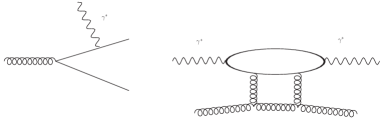
(a)                            (b)

Figure 6:   (a) Photon-gluon fusion. (b) Higher order contributions to photon-gluon $\rightarrow q\bar{q}$ fusion resolving the lower blob in fig.1. The lower part of the diagram must be extended to become a gluon ladder.

The longitudinal structure function, $F_{L}(x,Q^{2})$, in this low-$x$ or CDP approximation of pQCD solely depends on the gluon density, $g(x,Q^{2})$, [26]

$$F_{L}(x,Q^{2})=\frac{\alpha_{s}(Q^{2})}{3\pi}\sum_{q}Q^{2}_{q}\cdot 6I_{g}(x,Q^{2})$$ (2.106)

with

$$I_{g}(x,Q^{2})\equiv\int^{1}_{x}\frac{dy}{y}\left(\frac{x}{y}\right)^{2}\left(1-\frac{x}{y}\right)yg(y,Q^{2}).$$ (2.107)

where $G(y,Q^{2})\equiv yg(y,Q^{2})$. For a wide range of different gluon distributions, independently of their specific form, the integration in (2.107) yields a result that is proportional to the gluon density at a rescaled value $x/\xi_{L}$ [26] i.e.

$$F_{L}(\xi_{L}x,Q^{2})=\frac{\alpha_{s}(Q^{2})}{3\pi}\sum_{q}Q^{2}_{q}G(x,Q^{2}).$$ (2.108)

The rescaling factor $\xi_{L}$ in (2.108) has the preferred value of $\xi_{L}\cong 0.40$ [26]. The interaction of the longitudinally polarized photon with the quark (antiquark) originating from gluon $\rightarrow q\bar{q}$ splitting, via $F_{L}(\xi_{L}x,Q^{2})$, in good approximation thus fully determines the $x$ and $Q^{2}$ dependence of the gluon distribution function.

We turn to the structure function $F_{2}(x,Q^{2})$. In the DIS scheme of pQCD, at low $x$ and sufficiently large $Q^{2}$, $F_{2}(x,Q^{2})$ is proportional to the singlet or sea quark distribution $\sum(x,Q^{2})$,

$$\sum(x,Q^{2})=\sum^{n_{f}}_{q=1}(q_{q}(x)+\bar{q}_{q}(x)).$$ (2.109)

For four flavors of quarks, $n_{f}=4$, and flavor-blind quark distributions, the structure function is given by

$$F_{2}(x,Q^{2})=x\sum(x,Q^{2})\frac{1}{4}\sum_{q}Q^{2}_{q}=\frac{5}{18}x\sum(x,Q^{2}).$$ (2.110)

In the CDP approximation, $\gamma^{*}$ gluon $\rightarrow q\bar{q}$ fusion, the evolution of $F_{2}(x,Q^{2})$ with $Q^{2}$ is determined by the gluon distribution according to [12]

$$\frac{\partial F_{2}(x,Q^{2})}{\partial\ln Q^{2}}=\frac{\alpha_{s}(Q^{2})}{\pi}\sum_{q}Q^{2}_{q}\int^{1}_{x}dzP_{qg}(z)G\left(\frac{x}{z},Q^{2}\right),$$ (2.111)

where in leading order of pQCD

$$P_{qg}(z)=P_{qg}^{(0)}=\frac{1}{2}(z^{2}+(1-z)^{2}).$$ (2.112)

The evolution equation (2.111), again for a wide range of choices for the gluon distribution, may be represented by the proportionality [27]

$$\frac{\partial F_{2}(\xi_{2}x,Q^{2})}{\partial\ln Q^{2}}=\frac{\alpha_{s}(Q^{2})}{3\pi}\sum_{q}Q^{2}_{q}G(x,Q^{2}).$$ (2.113)

The rescaling factor in this case is given by $\xi_{2}\cong 0.50$ [27].

The validity of (2.108) and (2.113) and the values of the rescaling factors $(\xi_{L},\xi_{2})=(0.40,0.50)$ will be reexamined below by evaluating the relations (2.106) for $F_{L}(x,Q^{2})$ and (2.111) for $F_{2}(x,Q^{2})$ for the specific gluon distribution to be obtained by requiring consistency with the CDP approach.

We introduce the ratio of $F_{2}(x,Q^{2})$ and $F_{L}(x,Q^{2})$ by employing the form of this ratio in (2.59 ), but allowing for a potential dependence of $\rho\equiv\rho(x,Q^{2})$ on the kinematic variables $x$ and $Q^{2}$,

$$F_{L}(x,Q^{2})=\frac{1}{2\rho+1}F_{2}(x,Q^{2}).$$ (2.114)

Replacing the right-hand side of (2.113) by $F_{L}(\xi_{L}x,Q^{2})$ from (2.108), and subsequently replacing $F_{L}(\xi_{L}x,Q^{2})$ by $F_{2}(\xi_{L}x,Q^{2})$ according to the defining relation (2.114), the evolution equation (2.113) becomes

$$(2\rho+1)\frac{\partial}{\partial\ln Q^{2}}F_{2}\left(\frac{\xi_{2}}{\xi_{L}}x,Q^{2}\right)=F_{2}(x,Q^{2}),$$ (2.115)

or, in terms of the flavor singlet distribution (2.109) according to (2.110),

$$(2\rho+1)\frac{\partial}{\partial\ln Q^{2}}\frac{\xi_{2}}{\xi_{L}}\sum\left(\frac{\xi_{2}}{\xi_{L}}x,Q^{2}\right)=\sum(x,Q^{2}).$$ (2.116)

By alternatively replacing $F_{L}(x,Q^{2})$ in (2.114) by the gluon distribution from (2.108), upon inserting the resulting expression for $F_{2}(x,Q^{2})$ into the evolution equation (2.113), we find an evolution equation for the gluon density that reads

$$\frac{\partial}{\partial\ln Q^{2}}(2\rho+1)\alpha_{s}(Q^{2})G\left(\frac{\xi_{2}}{\xi_{L}}x,Q^{2}\right)=\alpha_{s}(Q^{2})G(x,Q^{2}).$$ (2.117)

Comparing (2.117) with (2.116), we conclude: if and only if

$$(2\rho+1)={\rm const.},$$ (2.118)

the evolution of the gluon density multiplied by $\alpha_{s}(Q^{2})$ in (2.117) coincides with the quark-singlet evolution according to (2.115) and (2.116).

Identical evolution of the $q\bar{q}$ sea originating from $\gamma^{*}$ gluon $\rightarrow q\bar{q}$ fusion (fig.6a) and the gluon distribution multiplied by $\alpha_{s}(Q^{2})$ appears as natural consequence of the fact that the $q\bar{q}$ state seen by the photon originates from the gluon: the evolution of the sea distribution, measured by the interaction with the photon, directly yields the evolution of the gluon distribution.

In the CDP, according to Section 2.4, specifically according to (2.63), and supported by the experimental results in fig.4, the structure function $F_{2}(x,Q^{2})$ for $x<0.1$ and $Q^{2}$ sufficiently large, depends on the single variable $W^{2}$,

$$F_{2}(x,Q^{2})=F_{2}(W^{2}=\frac{Q^{2}}{x}).$$ (2.119)

Independently of the specific form of the functional dependence of $F_{2}(x,Q^{2})$ on $W^{2}$, according to (2.119), the $Q^{2}$ dependence and the $x$ dependence of $F_{2}(x,Q^{2})$ are intimately related to each other. This is a consequence of the $W$ dependence of the dipole cross section in (2.1), compare (2.78) and (2.61). In terms of the energy variable $W$, the evolution equation (2.115) becomes

$$(2\rho_{W}+1)\frac{\partial}{\partial\ln W^{2}}F_{2}\left(\frac{\xi_{L}}{\xi_{2}}W^{2}\right)=F_{2}(W^{2}).$$ (2.120)

Since according to (2.1) the longitudinal as well as the transverse photoabsorption cross section depend on $W^{2}$, also the potential dependence of $\rho$ on $x$ and $Q^{2}$ is restricted to $W$, and in (2.120) , this is indicated by $\rho_{W}$.

We assume a power-law dependence for $F_{2}(W^{2})$ on $W^{2}$,

$$F_{2}(W^{2})\sim(W^{2})^{C_{2}}=\left(\frac{Q^{2}}{x}\right)^{C_{2}}.$$ (2.121)

We note that the dependence of $F_{2}(x,Q^{2})=F_{2}(W^{2})$ in (2.121) on a fixed (i.e. $Q^{2}$-independent) constant power $C_{2}$ of $1/x$ coincides with the $x\rightarrow 0$ so-called “hard” Pomeron solution [28] of pQCD that rests on a $(1/x)^{\lambda}$ input assumption for the flavor-singlet quark as well as the gluon distribution ($\lambda={\rm const})$. A fixed power of $1/x$, as $(1/x)^{\epsilon_{0}}$, also appears in the Regge approach to DIS based on a linear combination of a “soft” and a “hard” Pomeron, with the fit parameter of the hard Pomeron contribution being given by $\epsilon_{0}\cong 0.43$ [29].

It is a unique feature of the CDP, however, that the $1/x$ dependence and the $Q^{2}$ dependence of $F_{2}(x,Q^{2})$ (for $x<0.1$ and $Q^{2}$ sufficiently large, $Q^{2}\geq 10{\rm GeV}^{2}$) are determined by one and the same constant power $C_{2}$, compare (2.121).

Inserting the power-law (2.121) into the evolution equation (2.120), we find the constraint

$$(2\rho_{W}+1)C_{2}\left(\frac{\xi_{L}}{\xi_{2}}\right)^{C_{2}}=1.$$ (2.122)

Consistency of the power law (2.121) for the $W$ dependence with the flavor-singlet evolution (2.120) thus implies the remarkable constraint (2.122) that connects the exponent $C_{2}$ of the $1/x$ dependence with the longitudinal-to-transverse ratio of the photoabsorption cross sections, $2\rho_{W}$, or, equivalently with the ratio of $F_{2}(x,Q^{2})$ and $F_{L}(x,Q^{2})$ in (2.114). Constancy of $C_{2}$ implies constancy of $\rho_{W}=\rho={\rm const}$, and vice versa.

In the CDP, from (2.56), $\rho$ has the constant and fixed value of $\rho=4/3$. With this CDP value of $\rho=4/3$, we find from (2.122) (compare also [25])

$$C_{2}=\frac{1}{2\rho+1}\left(\frac{\xi_{2}}{\xi_{L}}\right)^{C_{2}}=0.29$$ (2.123)

where the preferred value of $\xi_{2}/\xi_{L}=0.5/0.4=1.25$ was inserted. We note that the (ad hoc) variation of this value in the interval $1\leq\xi_{2}/\xi_{L}\leq 1.5$ around the above value of $\xi_{2}/\xi_{L}=1.25$ yields $0.27\leq C_{2}\leq 1.31$. The result $C_{2}=0.29$ accordingly is fairly insensitive under variation of the rescaling factors $\xi_{2}$ and $\xi_{L}$.

We specify (2.121) by adopting the theoretical result for the exponent $C_{2}=0.29$ from (2.123) and by introducing a proportionality constant, $f_{2}$,

$$F_{2}(W^{2})=f_{2}\cdot\left(\frac{W^{2}}{1{\rm GeV}^{2}}\right)^{C_{2}=0.29}.$$ (2.124)

Via an eye-ball fit to the experimental data for $F_{2}(W^{2})$ as a function of $1/W^{2}$ in fig. 4a, we find

$$f_{2}=0.063.$$ (2.125)

The theoretical prediction (2.124) with (2.125) is shown in fig.4a. A detailed comparison with the experimental data, separately for distinct values of $Q^{2}$ in the relevant range of $10{\rm GeV}^{2}\leq Q^{2}\leq 100{\rm GeV}^{2}$ shows agreement with the single-free-parameter fit (2.124) to the structure function $F_{2}(W^{2})$ in (2.124) for $10{\rm GeV}^{2}\leq Q^{2}\leq 100{\rm GeV}^{2}$. Compare the discussion in Section 5, in particular figs.16 and 17.

According to (2.110), the flavor-singlet quark or sea distribution is proportional to the structure function $F_{2}(W^{2})$,

$$x\sum(x,Q^{2})=\frac{18}{5}f_{2}\cdot\left(\frac{W^{2}}{1{\rm GeV}^{2}}\right)^{C_{2}=0.29}.$$ (2.126)

Employing the proportionality (2.108) of the gluon distribution to the longitudinal structure function $F_{L}(\xi_{L}x,Q^{2})$, and expressing $F_{L}(\xi_{L}x,Q^{2})$ in terms of $F_{2}(\xi_{L}x,Q^{2})$ according to (2.114), we find that also the gluon distribution can be directly deduced from the experimental data for the structure function $F_{2}(x,Q^{2})=F_{2}(W^{2}=Q^{2}/x)$,

$$\alpha_{s}(Q^{2})G(x,Q^{2}) = \frac{3\pi}{\sum_{q}Q^{2}_{q}}F_{L}(\xi_{L}x,Q^{2})$$

$$= \frac{3\pi}{\sum_{q}Q^{2}_{q}}\frac{1}{(2\rho+1)}F_{2}(\xi_{L}x,Q^{2})$$

$$= \frac{3\pi}{\sum_{q}Q^{2}_{q}(2\rho+1)}\frac{f_{2}}{\xi_{L}^{C_{2}=0.29}}\left(\frac{W^{2}}{1{\rm GeV}^{2}}\right)^{C_{2}=0.29},$$

where (2.124) was inserted in the last step.

This is the appropriate point to add a remark, as previously announced, on the validity of the representations (2.108) and (2.113) in terms of the rescaling factors $(\xi_{L},\xi_{2})$. It will turn out that indeed without loss of generality (2.106) and (2.111) for our gluon distribution may be replaced by (2.108) and (2.113).

Inserting the gluon distribution (2.7) into the representations of $F_{L}(x,Q^{2})$ and $F_{2}(x,Q^{2})$ in (2.106) and (2.111), one may explicitly test the validity of the proportionalities to the gluon distribution in (2.108) and (2.113) that originate from (2.106) and (2.111). One finds that the above choice of the rescaling factors, $(\xi_{L},\xi_{2})=(0.4,0.5)$, yields a small discrepancy between the evaluation of the integrals over the gluon distribution and the representation in terms of the rescaling factors that amounts to about 4% and 6.5 % for $F_{L}(x,Q^{2})$ and $F_{2}(x,Q^{2})$, respectively. The discrepancy is reduced to less than 0.5% , for the choice of $(\xi_{L},\xi_{2})=(0.45,0.40)$. This implies a change of $C_{2}=0.29$ to $C_{2}=0.26$ in (2.123), close to the value of $C_{2}=0.27\pm 0.01$ found in the fit in refs.[11, 21]. For the comparison with the experimental data, the difference between $C_{2}=0.26$ and $C_{2}=0.29$ is not very important. We use $C_{2}=0.29$ in fig.4a and in the more extensive comparison with the experimental data in figs.16 and 17 in Section 5.

Figure 7: The gluon-distribution function from (2.7) compared with the gluon distributions from the hard-Pomeron part of a Regge fit [29] to $F_{2}(x,Q^{2})$, and from the $F_{2}(x,Q^{2})$ fits GRV [31], CTEQ [33] and MSTW[34].

In fig.7, we compare our gluon distribution from (2.7) with various gluon distributions obtained in fits to the experimental results for $F_{2}(x,Q^{2})$. Compare refs.[29, 31] and the Durham Data Base [32]. The gluon distributions from the various fits were multiplied by $\alpha_{s}(Q^{2})$, where

$$\alpha_{s}^{NLO}(Q^{2})=\frac{1}{bt}\left[1-\frac{b^{\prime}\ln t}{bt}\right].$$ (2.128)

with

$$b=\frac{33-2n_{f}}{12\pi},~{}~{}~{}b^{\prime}=\frac{153-19n_{f}}{2\pi(33-2n_{f})},$$ (2.129)

and $t=\ln(Q^{2}/\Lambda^{2}_{QCD}),n_{f}=4$ and $\Lambda_{QCD}=340{\rm MeV}$ corresponding to $\alpha_{s}(M^{2}_{Z})=0.113$.

According to fig.7, there is a considerable spread between the gluon-distribution functions extracted from experimental data of the structure function $F_{2}(x,Q^{2})$ by different collaborations. The gluon-distribution function corresponding to the hard Pomeron of the Regge fit [29] in general lies above our result. The results from the so-called global analysis by the CTEQ [33] and MSTW [34] collaborations are lower than ours. The fact that our results are fairly close to the results from GRV [30] seems no accident and deserves further examination.

Our relation (2.7) obtained as a consequence of the low-$x$ pQCD approximations (2.106) and (2.111) and the $W$ dependence of $F_{L,2}(x,Q^{2})=F_{L,2}(W^{2})$ from the CDP is transparent and simple as far as the underlying assumptions are concerned. The extracted gluon distribution only depends on the single normalization parameter $f_{2}$ that was adjusted to the experimental data. The gluon distribution can directly be read off from the experimental data for $F_{2}(W^{2}=Q^{2}/x)$ shown in fig.4 by multiplication of these data with the constant given in (2.7).

We end this Section with the following summarizing comments:

• The starting point for our extraction of the gluon distribution is the low-$x$ approximation of the pQCD-improved parton model that relates the gluon distribution to the longitudinal structure function, $F_{L}(x,Q^{2})$, compare (2.106). This relation is supplemented by the $W$-dependence of the structure functions $F_{L}(W^{2}=Q^{2}/x)$ and $F_{2}(W^{2}=Q^{2}/x)$ and their proportionality via the constant factor of $1/(2\rho+1)$, both the $W$ dependence and the proportionality being extracted from the CDP and being supported empirically. Finally, a power-law dependence, $F_{2}\sim(W^{2})^{C_{2}}=(Q^{2}/x)^{C_{2}}$ is inserted, with $C_{2}=0.29$ predicted from sea-quark evolution. The extraction of the gluon distribution depends on only one fitted normalization constant, $f_{2}$.

• The gluon distribution resulting from (2.7) lies within the range of gluon distributions available in the literature. We note that our extraction of the gluon distribution from the data on $F_{2}(x,Q^{2})=F_{2}(W^{2}=Q^{2}/x)$ is not based on a resolution of the $ggpp$ vertex, the lower blob in fig.1. The consistency of our gluon distribution with the ones in the literature indicates that the gluon distribution does not as sensitively depend on details of the structure of the $ggpp$ vertex as usually expected, assumed or elaborated upon. Compare the BFKL approach [35] to DIS at low $x$, as well as the double asymptotic scaling (DAS) solution [36, 37, 38] of DGLAP evolution [12] based on replacing the unresolved lower part of the diagram in fig.1 by the lower part of the diagram in fig.6b that has to be extended by a gluon ladder. We conjecture that our gluon distribution nevertheless, in the sense of a numerical approximation, is consistent with the DGLAP gluon evolution equation at low $x$ that supplements the evolution of the flavor-singlet quark distribution solely employed in our analysis.

• As mentioned, our $1/x$ dependence (2.7), $(2\rho+1)\alpha_{s}(Q^{2})xg(x,Q^{2})\sim x\sum(x,Q^{2})\sim(1/x)^{C_{2}}$ with fixed exponent $C_{2}$, is closely related to DGLAP evolution with the input constraint of a hard Pomeron [28]. We differ from ref.[28] insofar, as we have the necessary constraint of $(2\rho+1)={\rm const}$, compare (2.122), while the analysis of ref.[28] led to $(2\rho+1)\alpha_{s}(Q^{2})={\rm const.}$.

• Our $(1/x)^{C_{2}}$ dependence is analogous to the $(1/x)$ dependence of the hard Pomeron component of the Regge approach [29]. However, we predict $C_{2}=0.29$ from sea-quark evolution, the value being consistent with experiment, while the analogous parameter $\epsilon_{0}\cong 0.43$ in the Regge approach is a pure fit-parameter. Moreover, the CDP contains a smooth transition to low $Q^{2}$, including $Q^{2}=0$, rather than relying on the addition of a soft Pomeron. In the language of Pomeron exchange, the CDP only knows of a single Pomeron which is relevant for both small and large values of $Q^{2}$.

3 Models for the Dipole Cross Section

In Section 2, without adopting a specific parameterization for the dipole cross section, we found the proportionalities (2.6) of the total photoabsorption cross section to $\ln(1/\eta(W^{2},Q^{2}))$, for $\eta(W^{2},Q^{2})\ll 1$, and to $1/\eta(W^{2},Q^{2})$ for $\eta(W^{2},Q^{2})\gg 1$. Any specific parameterization of the dipole cross section has to interpolate between these two limits.

In Section 3.1, we will remind ourselves of a previously employed ansatz for the dipole cross section that implies $R(W^{2},Q^{2})=1/2$ at large $Q^{2}$ for the ratio of $R(W^{2},Q^{2})=\sigma_{\gamma^{*}_{L}p}(W^{2},Q^{2})/\sigma_{\gamma^{*}_{T}p}(W^{2},Q^{2})$. In Section 3.2, we introduce a more general ansatz that allows for the transverse-size reduction and associated enhancement of the transverse relative to the longitudinal photoabsorption cross section from Section 2.3.

3.1 A Dipole Cross Section Implying $R=0.5$

The ansatz for the dipole cross section in (2.1), previously employed in a successful fit to the experimental data on the total cross section, $\sigma_{\gamma^{*}p}(W^{2},Q^{2})$, is given by [11]

$$\sigma_{(q\bar{q})p}(\vec{r}_{\bot},z(1-z),W^{2})=\sigma^{(\infty)}(W^{2})\left(1-J_{0}\left(r_{\bot}\sqrt{z(1-z)}\Lambda_{sat}(W^{2})\right)\right),$$ (3.1)

where $\sigma^{(\infty)}(W^{2})$ is of hadronic size and weakly dependent on $W$, while $\Lambda^{2}_{sat}(W^{2})$ increases as a small power of $W^{2}$. Since the cross section (3.1) depends on the product $\vec{r}^{~{}\prime}_{\bot}=\vec{r}_{\bot}\sqrt{z(1-z)}$, the longitudinal and transverse $J=1$ projections in (2.2) become identical,

$$\sigma_{(q\bar{q})^{J=1}_{L}p}\left(r^{\prime}_{\bot}\Lambda_{sat}(W^{2})\right)=\sigma_{(q\bar{q})^{J=1}_{T}p}\left(r^{\prime}_{\bot}\Lambda_{sat}(W^{2})\right)$$

$$=\sigma^{(\infty)}(W^{2})\left(1-J_{0}(r^{\prime}_{\bot}\Lambda_{sat}(W^{2})\right)$$ (3.2)

$$=\sigma^{(\infty)}(W^{2})\left\{\matrix{\frac{1}{4}\vec{r}^{~{}\prime 2}_{\bot}\Lambda^{2}_{sat}(W^{2}),~{}~{}~{}{\rm for}~{}\vec{r}^{~{}\prime 2}_{\bot}\Lambda^{2}_{sat}(W^{2})\to 0,\cr 1,~{}~{}~{}~{}~{}~{}~{}~{}~{}~{}~{}~{}~{}~{}~{}~{}~{}~{}~{}~{}~{}{\rm for}~{}\vec{r}^{~{}\prime 2}_{\bot}\Lambda^{2}_{sat}(W^{2})\to\infty.}\right.$$

With respect to momentum space, the ansatz (3.1), according to (2.2), corresponds to

$$\tilde{\sigma}(\vec{l}^{~{}2}_{\bot},z(1-z),W^{2})=\frac{\sigma^{(\infty)}(W^{2})}{\pi}\delta\left(\vec{l}^{~{}2}_{\bot}-z(1-z)\Lambda^{2}_{sat}(W^{2})\right).$$ (3.3)

Its $J=1$ projections, according to (2.45), are given by

$$\bar{\sigma}_{(q\bar{q})^{J=1}_{L}p}(\vec{l}^{~{}\prime 2}_{\bot},W^{2})=\bar{\sigma}_{(q\bar{q})^{J=1}_{T}p}(\vec{l}^{~{}\prime 2}_{\bot},W^{2})=$$

$$=\frac{\sigma^{(\infty)}(W^{2})}{\pi}\delta\left(\vec{l}^{~{}\prime 2}_{\bot}-\Lambda^{2}_{sat}(W^{2})\right).$$ (3.4)

Substitution of (3.3) and (3.4) into (2.2) and (2.44), respectively, takes us back to (3.1) and (3.2).

We remark that helicity independence, the equality of the cross sections for scattering of the $J=1$ projections for longitudinally and transversely polarized $(q\bar{q})^{J=1}$ states in (3.2) and (3.4), is a general consequence of the dependence of the ansatz (3.1) on the variable $r_{\bot}^{\prime}=r_{\bot}\sqrt{z(1-z)}$. Any dipole cross section in (2.1) fulfilling

$$\sigma_{(q\bar{q})p}(\vec{r}_{\bot},z(1-z),W^{2})=\sigma_{(q\bar{q})p}\left(\vec{r}_{\bot}\sqrt{z(1-z)},W^{2}\right),$$ (3.5)

together with color transparency (2.2), implies helicity independence and $R(W^{2},Q^{2})=1/2$ at large $Q^{2}$. Indeed, consistency of (3.5) with (2.2),

$$\sigma_{(q\bar{q})p}(r_{\bot}\sqrt{z(1-z)},W^{2})=\int d^{2}\vec{l}_{\bot}^{~{}\prime}z(1-z)\tilde{\sigma}(\vec{l}_{\bot}^{~{}\prime 2}z(1-z),z(1-z),W^{2})\cdot$$

$$\cdot\left(1-e^{-i\vec{l}_{\bot}^{~{}\prime}\cdot\vec{r}_{\bot}^{~{}\prime}}\right),$$ (3.6)

requires $z(1-z)\tilde{\sigma}(\vec{l}_{\bot}^{~{}\prime 2}z(1-z),z(1-z),W^{2})$ to be independent of $z(1-z)$. Under this constraint, (2.45) implies helicity independence and $R(W^{2},Q^{2})=1/2$ according to (2.47).

The ansatz (3.1) for the dipole cross section has to be supplemented by a constraint on the masses of the contributing $q\bar{q}$ fluctuations that is best incorporated by returning from transverse position space to momentum space. The constraint reads

$$m^{2}_{0}\leq M^{2}_{q\bar{q}},M^{\prime 2}_{q\bar{q}}\leq m^{2}_{1}(W^{2}),$$ (3.7)

where the notation, i.e. $M^{2}_{q\bar{q}},M^{\prime 2}_{q\bar{q}}$, for the masses of the $(q\bar{q})$ dipole states, indicates that incoming and outgoing $q\bar{q}$ masses in the forward Compton amplitude of fig.1 do not necessarily agree with each other. The lower bound, $m_{0}^{2}$, depends on the flavor of the actively contributing quarks. For up and down quarks the value of $m_{0}$ must be somewhat below the $\rho^{0}$ mass. The upper bound, $m^{2}_{1}(W^{2})$, depends on the available energy. In most applications of the CDP, the approximation of $m^{2}_{1}(W^{2})\rightarrow\infty$ is employed that restricts the kinematic range 2.of applicability of the CDP. For the present discussion we put $m^{2}_{1}(W^{2})\rightarrow\infty$. We will come back to a finite value of $m^{2}_{1}(W^{2})$ in Section 4.

According to dimensional analysis, with $m^{2}_{1}(W^{2})\rightarrow\infty$, the photoabsorption cross section resulting from (3.1) in addition to the dependence on $\eta(W^{2},Q^{2})=(Q^{2}+m^{2}_{0})/\Lambda^{2}_{\rm sat}(W^{2})$ will depend on $m^{2}_{0}/\Lambda^{2}_{\rm sat}(W^{2})$. For the realistic case of $m^{2}_{0}/\Lambda^{2}_{\rm sat}(W^{2})\ll 1$, the total photoabsorption cross section $\sigma_{\gamma^{*}p}(W^{2},Q^{2})=\sigma_{\gamma^{*}_{T}p}(W^{2},Q^{2})+\sigma_{\gamma^{*}_{L}p}(W^{2},Q^{2})$ takes the remarkably simple explicit form [11]

$$\sigma_{\gamma^{*}p}(W^{2},Q^{2}) = \sigma_{\gamma^{*}p}(\eta(W^{2},Q^{2}))+O\left(\frac{m^{2}_{0}}{\Lambda^{2}_{\rm sat}(W^{2})}\right)=$$ (3.8)

$$=\frac{\alpha R_{e^{+}e^{-}}}{3\pi}\sigma^{(\infty)}(W^{2})I_{0}(\eta)+O\left(\frac{m^{2}_{0}}{\Lambda^{2}_{\rm sat}(W^{2})}\right),$$

where

$$I_{0}(\eta(W^{2},Q^{2})) = \frac{1}{\sqrt{1+4\eta(W^{2},Q^{2})}}\ln\frac{\sqrt{1+4\eta(W^{2},Q^{2})}+1}{\sqrt{1+4\eta(W^{2},Q^{2})}-1}\cong$$

$$\cong \left\{\matrix{\ln\frac{1}{\eta(W^{2},Q^{2})}+O(\eta\ln\eta),~{}~{}{\rm for}~{}\eta(W^{2},Q^{2})\rightarrow\frac{m^{2}_{0}}{\Lambda^{2}_{\rm sat}(W^{2})},\cr\frac{1}{2\eta(W^{2},Q^{2})}+O\left(\frac{1}{\eta^{2}}\right),~{}{\rm for}~{}\eta(W^{2},Q^{2})\rightarrow\infty,}\right.$$

and

$$R_{e^{+}e^{-}}=3\sum_{q}Q^{2}_{q}.$$ (3.10)

As expected, since (3.1) fulfills color transparency, compare (3.2), the result (3.8) with (3.1) and $\sigma^{(\infty)}(W^{2})\cong{\rm const}$ constitutes an example for the general result in (2.82) and (2.92) from Section 2.5.

For further reference, we give the explicit parameterization of the ansatz (3.1) and the values of the parameters obtained in the fit to the experimental data. The “saturation scale”, $\Lambda^{2}_{sat}(W^{2})$ is given by [11, 21]

$$\Lambda^{2}_{sat}(W^{2})=B\left(\frac{W^{2}}{W^{2}_{0}}+1\right)^{C_{2}},$$ (3.11)

with

$$B = 2.24\pm 0.43~{}GeV^{2},$$

$$W^{2}_{0} = 1081\pm 124~{}GeV^{2},$$ (3.12)

$$C_{2} = 0.27\pm 0.01.$$

In good approximation, (3.11) becomes

$$\Lambda^{2}_{sat}(W^{2})=C_{1}\left(\frac{W^{2}}{1~{}GeV^{2}}\right)^{C_{2}},$$ (3.13)

with

$$C_{1}=0.34\pm 0.06{\rm GeV}^{2}$$ (3.14)

i.e. $\Lambda^{2}_{{\rm sat}}(W^{2})$ is in good approximation determined by only two parameters, the normalization scale $C_{1}$ and the exponent $C_{2}$.

The hadronic cross section, $\sigma^{(\infty)}(W^{2})$, was obtained [11] by requiring consistency with the Regge fit to the measured $Q^{2}=0$ photoproduction cross section. It determines the product of $R_{e^{+}e^{-}}\sigma^{(\infty)}(W^{2})$, where $R_{e^{+}e^{-}}=3\sum_{q}Q^{2}_{q}$. With three active flavors, $R_{e^{+}e^{-}}=2$, and

$$\sigma^{(\infty)}(W^{2})\cong 30mb=77.04~{}GeV^{-2}.$$ (3.15)

The value of the lower bound, $m^{2}_{0}$, in (3.7) is given by

$$m^{2}_{0}=0.15\pm 0.04GeV^{2}.$$ (3.16)

3.2 The Ansatz for the Dipole Cross Section implying $R=1/2\rho(\epsilon)$

Returning to the discussion in Section 2, compare in particular (2.23), we generalize (3.3) to become

$$\tilde{\sigma}(\vec{l}^{~{}2}_{\bot},z(1-z),W^{2})=\frac{\bar{\sigma}^{(\infty)}(W^{2})}{\pi}\delta\left(\vec{l}^{~{}2}_{\bot}-\frac{1}{6}\bar{\Lambda}^{2}_{sat}(W^{2})\right)\Theta(z(1-z)-\epsilon).$$ (3.17)

With respect to transverse position space, according to (2.2), we obtain from (3.17),

$$\sigma_{(q\bar{q})p}(r_{\bot},z(1-z),W^{2})=\bar{\sigma}^{(\infty)}(W^{2})\left(1-J_{0}(r_{\bot}\frac{\bar{\Lambda}_{\rm sat}(W^{2})}{\sqrt{6}})\right)\Theta(z(1-z)-\epsilon)$$

$$\cong\bar{\sigma}^{(\infty)}(W^{2})\Theta(z(1-z)-\epsilon)\left\{\matrix{\frac{1}{4}\frac{\bar{\Lambda}^{~{}2}_{\rm sat}(W^{2})}{6}\vec{r}_{\bot}^{~{}2},&{\rm for}~{}\vec{r}_{\bot}^{~{}2}\rightarrow 0,\cr 1,&{\rm for}~{}\vec{r}_{\bot}^{~{}2}\rightarrow\infty.}\right.$$ (3.18)

The $\delta$-function in (3.17), via $\bar{\Lambda}^{~{}2}_{sat}(W^{2})$, specifies the $W$-dependence of the integral $\int d\vec{l}^{~{}2}_{\bot}\vec{l}^{~{}2}_{\bot}~{}\tilde{\sigma}(\vec{l}^{~{}2}_{\bot},W^{2})$ that, according to (2.25), determines the photoabsorption cross section at large $Q^{2}$. The $\Theta$-function in (3.17), compare (2.23), provides the necessary $W$-dependent cut on $\vec{l}^{~{}\prime 2}_{\bot}=\vec{l}^{~{}2}_{\bot}/z(1-z)$. It forbids $q\bar{q}$ fluctuations of infinitely large mass to occur as a result of gluon absorption at finite energy, $W$. The $J=1$ projections of the ansatz (3.17), by substitution of (3.17) into (2.45), are found to be given by

$$\bar{\sigma}_{(q\bar{q})^{J=1}_{L,T}p}\left(\vec{l}^{~{}\prime 2}_{\bot},\bar{\Lambda}^{~{}2}_{sat}(W^{2})\right)=f_{L,T}\left(\vec{l}^{~{}\prime 2}_{\bot},\bar{\Lambda}^{~{}2}_{sat}(W^{2})\right)\cdot$$

$$~{}~{}~{}~{}~{}~{}~{}~{}\cdot\Theta\left(\vec{l}^{~{}\prime 2}_{\bot}-\frac{2}{3}\bar{\Lambda}^{~{}2}_{sat}(W^{2})\right)\Theta\left(a\bar{\Lambda}^{~{}2}_{sat}(W^{2})-\vec{l}^{~{}\prime 2}_{\bot}\right),$$ (3.19)

where

$$f_{L}\left(\vec{l}^{~{}\prime 2}_{\bot},\bar{\Lambda}^{~{}2}_{sat}(W^{2})\right)=\frac{\bar{\sigma}^{(\infty)}(W^{2})}{3\pi}\frac{\bar{\Lambda}^{~{}4}_{sat}(W^{2})}{\vec{l}^{~{}\prime 6}_{\bot}}\frac{1}{\sqrt{1-\frac{2\bar{\Lambda}^{~{}2}_{sat}(W^{2})}{3\vec{l}^{~{}\prime 2}_{\bot}}}},$$ (3.20)

and

$$f_{T}\left(\vec{l}^{~{}\prime 2}_{\bot},\bar{\Lambda}^{~{}2}_{sat}(W^{2})\right)=\frac{3\vec{l}^{~{}\prime 2}_{\bot}}{2\bar{\Lambda}^{~{}2}_{sat}(W^{2})}\left(1-\frac{1}{3}\frac{\bar{\Lambda}^{~{}2}_{sat}(W^{2})}{\vec{l}^{~{}\prime 2}_{\bot}}\right)f_{L}\left(\vec{l}^{~{}\prime 2}_{\bot},\bar{\Lambda}^{~{}2}_{sat}(W^{2})\right).$$ (3.21)

The constant $a$ in (3.19) is related to $\epsilon$ in (3.18) by $\epsilon=1/6a$, where $a\gg 1$. Comparison of (3.19) with (3.4) reveals that the peak as a function of $\vec{l}_{\bot}^{~{}\prime 2}$ at $\vec{l}_{\bot}^{~{}\prime 2}=\Lambda^{2}_{\rm sat}(W^{2})$ in (3.4) is replaced by a broad distribution in the interval $(2/3)\bar{\Lambda}^{2}_{\rm sat}(W^{2})\leq\vec{l}_{\bot}^{~{}\prime 2}\leq a\bar{\Lambda}^{2}_{\rm sat}(W^{2})$. For $\vec{l}^{~{}\prime 2}_{\bot}>\bar{\Lambda}^{~{}2}_{sat}(W^{2})$, the transverse part of the dipole cross section in (3.21) becomes enhanced by a factor of $\vec{l}_{\bot}^{~{}\prime 2}/\Lambda^{2}_{sat}(W^{2})$ relative to the longitudinal one.

Inserting the $J=1$ dipole cross section (3.19), with (3.20) and (3.21), into the large-$Q^{2}$ form of the photoabsorption cross section in (2.47), we find (with $Q^{2}\gg\bar{\Lambda}^{2}_{sat}(W^{2})$)

$$\sigma_{\gamma^{*}_{L,T}p}(W^{2},Q^{2})=\frac{\alpha}{\pi}\sum_{q}Q^{2}_{q}\frac{1}{Q^{2}}\frac{1}{6}\bar{\sigma}^{~{}(\infty)}(W^{2})\bar{\Lambda}^{~{}2}_{sat}(W^{2})\sqrt{1-\frac{2}{3a}}\left\{\matrix{1,\cr 2\rho\left(\epsilon=\frac{1}{6a}\right),}\right.$$ (3.22)

where $2\rho\left(\epsilon=\frac{1}{6a}\right)$ coincides with the result given in (2.27). Here, we assumed $m^{2}_{1}(W^{2})\rightarrow\infty$. The generalization to finite values of $m^{2}_{1}(W^{2})$ will be given in Section 4, compare (4.28).

The photoabsorption cross section (3.22) may be expressed in terms of the cross section $\sigma_{L}^{(\infty)}(W^{2})$ and the scale $\Lambda^{2}_{sat}(W^{2})$ introduced in Section (2.5) in terms of integrals over the longitudinal part of the $J=1$ dipole cross section. Compare (2.73) and (2.74). Evaluating (2.73) and (2.74) for the ansatz (3.19), we find

$$\sigma_{L}^{(\infty)}(W^{2}) =\bar{\sigma}^{~{}(\infty)}(W^{2})\left(1+\frac{1}{3a}\right)\sqrt{1-\frac{2}{3a}}$$

$$\cong\bar{\sigma}^{~{}(\infty)}(W^{2})\left(1-\frac{1}{9a^{2}}\right),~{}~{}~{}(a>1)$$

and

$$\Lambda^{2}_{sat}(W^{2})=\bar{\Lambda}^{2}_{sat}(W^{2})\frac{1}{1+\frac{1}{3a}}.$$ (3.24)

The photoabsorption cross section (3.22) may accordingly be written in terms of $\sigma^{\infty}_{L}(W^{2})$ and $\Lambda^{2}_{sat}(W^{2})$ to become

$$\sigma_{\gamma^{*}_{L,T}p}(W^{2},Q^{2}) = \frac{\alpha}{\pi}\sum_{q}Q^{2}_{q}\frac{1}{6}\sigma_{L}^{(\infty)}(W^{2})\frac{\Lambda^{2}_{sat}(W^{2})}{Q^{2}}\left\{\matrix{1\cr 2\rho\left(\epsilon=\frac{1}{6a}\right)}\right.,$$ (3.25)

$$(Q^{2}\gg\Lambda^{2}_{sat}(W^{2})).$$

The result (3.25) correctly coincides with the general result (2.78).

A comparison of (3.25) with (3.8) and the $\eta(W^{2},Q^{2})\rightarrow\infty$ limit in (3.1) shows that the large-$Q^{2}$ cross section (3.25) formally corresponds to the polarization-dependent replacement in (3.1) of

$$\Lambda^{2}_{sat}(W^{2})\rightarrow\left\{\matrix{\Lambda^{2}_{sat,L}(W^{2})=\Lambda^{2}_{sat}(W^{2}),\cr\Lambda^{2}_{sat,T}(W^{2})=\rho(\epsilon)\Lambda^{2}_{sat}(W^{2}).}\right.$$ (3.26)

combined with the substitution

$$\sigma^{(\infty)}(W^{2})\rightarrow\sigma_{L}^{(\infty)}(W^{2})$$ (3.27)

The justification of the resulting cross section (3.25) rests on the ansatz (3.18), since the dipole cross section in (2.1), and accordingly in (3.1) must be independent of the polarization indices $T$ and $L$ of $q\bar{q}$ dipole fluctuations. The replacement (3.26) with (3.27) is nevertheless illuminating for an intuitive understanding of the transition from (3.1) to the ansatz (3.17).

4 The Evaluation of the Photoabsorption Cross Section, Analytic Results.

For the evaluation of the ansatz for the photoabsorption cross section presented in Section 3, we return to momentum space. Inserting the representation for the longitudinal and the transverse part of the $J=1$ dipole cross section (2.44) into (2.39), and employing the momentum-space representation of the modified Bessel functions $K_{0,1}(r^{\prime}_{\bot}Q)$, one finds (compare Appendix A)

$$\sigma_{\gamma^{*}_{L}p}(W^{2},Q^{2})=\frac{\alpha R_{e^{+}e^{-}}}{3\pi}Q^{2}\int d\vec{l}^{~{}\prime 2}_{\bot}\bar{\sigma}_{(q\bar{q})^{J=1}_{L}p}(\vec{l}^{~{}\prime 2}_{\bot},W^{2})\cdot$$

$$\cdot\int dM^{2}\int dM^{\prime 2}w(M^{2},M^{\prime 2},\vec{l}^{~{}\prime 2}_{\bot})\left(\frac{1}{(Q^{2}+M^{2})^{2}}-\frac{1}{(Q^{2}+M^{2})(Q^{2}+M^{\prime 2})}\right)$$

(4.1)

and

$$\sigma_{\gamma^{*}_{T}p}(W^{2},Q^{2})=\frac{\alpha R_{e^{+}e^{-}}}{3\pi}\int d\vec{l}^{~{}\prime 2}_{\bot}\bar{\sigma}_{(q\bar{q})^{J=1}_{T}p}(\vec{l}^{~{}\prime 2}_{\bot},W^{2})\cdot$$

$$\cdot\int dM^{2}\int dM^{\prime 2}w(M^{2},M^{\prime 2},\vec{l}^{~{}\prime 2}_{\bot})\left(\frac{M^{2}}{(Q^{2}+M^{2})^{2}}-\frac{1}{2}\frac{M^{2}+M^{\prime 2}-\vec{l}^{~{}\prime 2}_{\bot})}{(Q^{2}+M^{2})(Q^{2}+M^{\prime 2})}\right).$$

(4.2)

In the transition from (2.39) to (4.1) and (4.2), we introduced the $q\bar{q}$ masses,

$$M^{2}=\frac{\vec{k}^{~{}2}_{\bot}}{z(1-z)}\equiv\vec{k}^{~{}\prime 2}_{\bot},$$ (4.3)

in terms of the quark transverse momentum, $\vec{k}_{\bot}$, and

$$M^{\prime 2}=\frac{(\vec{k}_{\bot}+\vec{l}_{\bot})^{2}}{z(1-z)},$$ (4.4)

in terms of the transverse momentum of the quark upon absorption of the gluon.

In (4.1) and (4.2), $R_{e^{+}e^{-}}=3\sum_{q}Q^{2}_{q}$, where the sum runs over the actively contributing quarks. The Jacobian $w(M^{2},M^{\prime 2},\vec{l}^{~{}\prime 2}_{\bot})$ in (4.1) and (4.2) is given by [6]

$$w(M^{2},M^{\prime 2},\vec{l}^{~{}\prime 2}_{\bot})=\frac{1}{2MM^{\prime}\sqrt{1-\cos^{2}\phi}}=\frac{1}{2M\sqrt{\vec{l}^{~{}\prime 2}_{\bot}}\sqrt{(1-\cos^{2}\vartheta)}},$$ (4.5)

where $\phi$ denotes the angle between $\vec{k}_{\bot}$ and $(\vec{k}_{\bot}+\vec{l}_{\bot})$, and $\vartheta$ denotes the angle between $\vec{k}_{\bot}$ and $\vec{l}_{\bot}$. Since

$$\cos^{2}\phi=\frac{1}{4M^{2}M^{\prime 2}}\left(M^{2}+M^{\prime 2}-\vec{l}_{\bot}^{~{}\prime 2}\right)$$ (4.6)

is symmetric under exchange of $M^{2}$ and $M^{\prime 2}$, also $w(M^{2},M^{\prime 2},\vec{l}^{~{}\prime 2}_{\bot})$ in (4.5) is symmetric under exchange of $M^{2}$ and $M^{\prime 2}$. The integrands in (4.1) and (4.2) may be cast into a form that is fully symmetric under exchange of $M^{2}$ and $M^{\prime 2}$, thus explicitly displaying the symmetry of the virtual forward-Compton-scattering amplitude from fig. 1. It describes the process $\gamma^{*}p\to\gamma^{*}p$ in terms of the “diagonal” transitions $M_{(q\bar{q})}\to M_{(q\bar{q})}$ and $M^{\prime}_{(q\bar{q})}\to M^{\prime}_{(q\bar{q})}$ and the “off-diagonal” ones $M_{(q\bar{q})}\leftrightarrow M^{\prime}_{(q\bar{q})}$, in a symmetric manner.

The integrations in (4.1) and (4.2) have to fulfill the restrictions

$$m^{2}_{0}\leq M^{2},M^{\prime 2}\leq m^{2}_{1}(W^{2}).$$ (4.7)

The lower bound, $m^{2}_{0}$, in (4.7) corresponds to vanishing $\gamma^{*}\to q\bar{q}$ transitions, as soon as $\vec{k}_{\bot}^{~{}2}$ (and $(\vec{k}_{\bot}+\vec{l}_{\bot})^{2}$ ) become sufficiently small. A vanishing value of $\vec{k}^{~{}2}_{\bot}$ would imply contributions to the Compton-forward-scattering amplitude of states of unbounded transverse size that do not occur as a consequence of quark confinement. Via quark-hadron duality in $e^{+}e^{-}$ annihilation, the value of $m_{0}$ must be somewhat below the $\rho^{0}$ mass. The upper limit, $m^{2}_{1}(W^{2})$, in (4.7) follows from the restriction on the lifetime, (2.60), of a hadronic $q\bar{q}$ fluctuation that requires $M^{2}$ and $M^{\prime 2}$ to be strongly bounded for any finite value of the energy, $W$. Quantitatively, for a typical HERA energy of $W=225GeV$, the crude estimate of $M^{2}_{q\bar{q}}/W^{2}=0.01$ requires $m_{1}(W)=22.5GeV$. This value is approximately consistent with the mass range of the diffractive continuum that is directly related to the scattering of $q\bar{q}$ fluctuations relevant for the total photoabsorption cross section. Obviously, the mass bound, $m^{2}_{1}=m^{2}_{1}(W^{2})$, increases with increasing energy.

For the evaluation of (4.1) and (4.2) with the restriction of (4.7) on $M^{2}$ and $M^{\prime 2}$, it is convenient to replace the integration over $dM^{\prime 2}$ by an integration over $d\vartheta$. Noting that

$$M^{\prime 2}(M^{2},\vec{l}^{~{}\prime 2}_{\bot},\cos\vartheta)=M^{2}+\vec{l}^{~{}\prime 2}_{\bot}+2M\sqrt{\vec{l}_{\bot}^{~{}\prime 2}}\cos\vartheta,$$ (4.8)

and

$$\frac{\partial M^{\prime 2}(M^{2},\vec{l}^{~{}\prime 2}_{\bot},\cos\vartheta)}{\partial\vartheta}=-\frac{1}{w(M^{2},M^{\prime 2},\vec{l}^{~{}\prime 2}_{\bot})},$$ (4.9)

upon incorporating the restrictions in (4.7), the integrations in (4.1) and (4.2) simplify to become

$$\int dM^{2}\int dM^{\prime 2}w(M^{2},M^{\prime 2},\vec{l}^{~{}\prime 2}_{\bot})=$$ (4.10)

$$=\int^{m^{2}_{1}(W^{2})}_{m^{2}_{0}}dM^{2}\int^{\pi}_{0}d\vartheta-\int^{(\sqrt{\vec{l}^{~{}\prime 2}_{\bot}}+m_{0})^{2}}_{(\sqrt{\vec{l}^{~{}\prime 2}_{\bot}}-m_{0})^{2}}dM^{2}\int^{\pi}_{\vartheta_{0}(M^{2},\vec{l}^{~{}\prime 2}_{\bot})}d\vartheta$$

$$-\int^{m^{2}_{1}(W^{2})}_{(m_{1}(W^{2})-\sqrt{\vec{l}^{~{}\prime 2}_{\bot}})^{2}}dM^{2}\int^{\vartheta_{1}(M^{2},\vec{l}^{~{}\prime 2}_{\bot})}_{0}d\vartheta.$$

2. The first term in (4.10) takes care of the bound on $M^{2}$ in (4.7), ignoring, however, the restriction on $\vartheta$ induced by the bound on $M^{\prime 2}$. The second and the third term in (4.10) correct for this ignored restriction on $M^{\prime 2}$. The bounds on the angles, $\vartheta_{0}(M^{2},\vec{l}^{~{}\prime 2}_{\bot})$ and $\vartheta_{1}(M^{2},\vec{l}^{~{}\prime 2}_{\bot})$ in (4.10), are obtained from the lower and the upper bound on $M^{\prime 2}(M^{2},\vec{l}^{~{}\prime 2}_{\bot},\cos\vartheta)$ implied by (4.8) and are given by

$$\cos\vartheta_{0,1}(M^{2},\vec{l}^{~{}\prime 2}_{\bot})=\frac{m^{2}_{0,1}-M^{2}-\vec{l}^{~{}\prime 2}_{\bot}}{2M\sqrt{\vec{l}^{~{}\prime 2}_{\bot}}}.$$ (4.11)

Here $m^{2}_{1}$ stands for $m^{2}_{1}\equiv m^{2}_{1}(W^{2})$. In terms of the $dM^{2}d\vartheta$ integration (4.10), the photoabsorption cross sections in (4.1) and (4.2) become

$$\sigma_{\gamma^{*}_{L}p}(W^{2},Q^{2})=\frac{\alpha R_{e^{+}e^{-}}}{3\pi}\int d\vec{l}^{~{}\prime 2}_{\bot}\bar{\sigma}_{(q\bar{q})^{J=1}_{L}p}(\vec{l}^{~{}\prime 2}_{\bot},W^{2})\cdot$$ (4.12)

$$\cdot\int dM^{2}\int d\vartheta\left(\frac{Q^{2}}{(Q^{2}+M^{2})^{2}}-\frac{Q^{2}}{(Q^{2}+M^{2})(Q^{2}+M^{\prime 2}(M^{2},\vec{l}^{~{}\prime 2}_{\bot},\cos\vartheta))}\right)$$

and

$$\sigma_{\gamma^{*}_{T}p}(W^{2},Q^{2})=\frac{\alpha R_{e^{+}e^{-}}}{3\pi}\int d\vec{l}^{~{}\prime 2}_{\bot}\bar{\sigma}_{(q\bar{q})^{J=1}_{T}p}(\vec{l}^{~{}\prime 2}_{\bot},W^{2})\cdot$$ (4.13)

$$\cdot\int dM^{2}\int d\vartheta\left(\frac{M^{2}}{(Q^{2}+M^{2})^{2}}-\frac{M^{2}+M^{\prime 2}(M^{2},\vec{l}^{~{}\prime 2}_{\bot},\cos\vartheta)-\vec{l}^{~{}\prime 2}_{\bot}}{2(Q^{2}+M^{2})(Q^{2}+M^{\prime 2}(M^{2},\vec{l}^{~{}\prime 2}_{\bot},\cos\vartheta))}\right).$$

The integrations in (4.12) and (4.13), according to (4.10), lead to a sum of three terms,

$$\sigma_{\gamma^{*}_{L,T}p}(W^{2},Q^{2})=\sigma^{dom}_{\gamma^{*}_{L,T}p}(W^{2},Q^{2})+\Delta\sigma^{(m^{2}_{0})}_{\gamma^{*}_{L,T}p}(W^{2},Q^{2})+\Delta\sigma^{(m^{2}_{1}(W^{2}))}_{\gamma^{*}_{L,T}p}(W^{2},Q^{2}).$$ (4.14)

The first term will be dominant. The correction due to the lower bound $m^{2}_{0}$ will turn out to be small, of order 1 %. The third term in (4.14) will be found to yield a somewhat larger contribution, of order 10 %, dependent on the values of the kinematical variables.

For the dominant term, the integration of (4.12) and (4.13) with the integration domain given by the first term in (4.10), can be carried out analytically. We concentrate on the dominant term, and for the correction terms refer to Appendix B.

Upon integration over $d\vartheta$ of (4.12) and (4.13), the dominant contributions to the photoabsorption cross section become [16]

$$\sigma^{dom}_{\gamma^{*}_{L}p}(W^{2},Q^{2})=\frac{\alpha R_{e^{+}e^{-}}}{3}\int d\vec{l}^{~{}\prime 2}_{\bot}\bar{\sigma}_{(q\bar{q})^{J=1}_{L}p}(\vec{l}^{~{}\prime 2}_{\bot},W^{2})\cdot$$ (4.15)

$$\cdot\int^{m^{2}_{1}(W^{2})}_{m^{2}_{0}}dM^{2}\left(\frac{Q^{2}}{(Q^{2}+M^{2})^{2}}-\frac{Q^{2}}{(Q^{2}+M^{2})\sqrt{X(M^{2},\vec{l}^{~{}\prime 2}_{\bot},Q^{2})}}\right),$$

and

$$\sigma^{dom}_{\gamma^{*}_{T}p}(W^{2},Q^{2})=\frac{\alpha R_{e^{+}e^{-}}}{3}\int d\vec{l}^{~{}\prime 2}_{\bot}\bar{\sigma}_{(q\bar{q})^{J=1}_{T}p}(\vec{l}^{~{}\prime 2}_{\bot},W^{2})\cdot$$

$$\cdot\int^{m^{2}_{1}(W^{2})}_{m^{2}_{0}}\frac{dM^{2}}{2}\left(\frac{1}{(Q^{2}+M^{2})}-\frac{2Q^{2}}{(Q^{2}+M^{2})^{2}}-\frac{1}{\sqrt{X(M^{2},\vec{l}^{~{}\prime 2}_{\bot},Q^{2})}}+\right.$$

$$\left.\frac{2Q^{2}+\vec{l}^{~{}\prime 2}_{\bot}}{(Q^{2}+M^{2})\sqrt{X(M^{2},\vec{l}^{~{}\prime 2}_{\bot},Q^{2})}}\right),$$ (4.16)

where

$$X(M^{2},\vec{l}^{~{}\prime 2}_{\bot},Q^{2})\equiv(M^{2}-\vec{l}^{~{}\prime 2}_{\bot}+Q^{2})^{2}+4Q^{2}\vec{l}^{~{}\prime 2}_{\bot}.$$ (4.17)

Carrying out the integration over $dM^{2}$ in (4.15) and (4.16), we finally obtain

$$\sigma^{dom}_{\gamma^{*}_{L,T}p}(W^{2},Q^{2})=\frac{\alpha R_{e^{+}e^{-}}}{3}\int d\vec{l}^{~{}\prime 2}_{\bot}\bar{\sigma}_{(q\bar{q})^{J=1}_{L,T}p}(\vec{l}^{~{}\prime 2}_{\bot},W^{2})\cdot$$

$$\cdot\left(I_{L,T}(\vec{l}^{~{}\prime 2}_{\bot},m^{2}_{1}(W^{2}),Q^{2})-I_{L,T}(\vec{l}^{~{}\prime 2}_{\bot},m^{2}_{0},Q^{2})\right),$$

(4.18)

where $I_{L,T}(\vec{l}^{~{}\prime 2}_{\bot},M^{2},Q^{2})$ denotes the indefinite integrals over $dM^{2}$ in (4.15) and (4.16). They are given by

$$I_{L}(\vec{l}^{~{}\prime 2}_{\bot},M^{2},Q^{2})=\frac{-Q^{2}}{Q^{2}+M^{2}}+\frac{Q^{2}}{\sqrt{\vec{l}^{~{}\prime 2}_{\bot}(\vec{l}^{~{}\prime 2}_{\bot}+4Q^{2})}}\cdot$$ (4.19)

$$\cdot\ln\frac{\sqrt{\vec{l}^{~{}\prime 2}_{\bot}(\vec{l}^{~{}\prime 2}_{\bot}+4Q^{2})}\sqrt{X(M^{2},\vec{l}^{~{}\prime 2}_{\bot},Q^{2})}+\vec{l}^{~{}\prime 2}_{\bot}(3Q^{2}-M^{2}+\vec{l}^{~{}\prime 2}_{\bot})}{Q^{2}+M^{2}}$$

and

$$I_{T}(\vec{l}^{~{}\prime 2}_{\bot},M^{2},Q^{2})=$$ (4.20)

$$=\frac{Q^{2}}{Q^{2}+M^{2}}+\frac{1}{2}\ln\frac{Q^{2}+M^{2}}{\sqrt{X(M^{2},\vec{l}^{~{}\prime 2}_{\bot},Q^{2})}+M^{2}-\vec{l}^{~{}\prime 2}_{\bot}+Q^{2}}-\frac{2Q^{2}+\vec{l}^{~{}\prime 2}_{\bot}}{2\sqrt{\vec{l}^{~{}\prime 2}_{\bot}(\vec{l}^{~{}\prime 2}_{\bot}+4Q^{2})}}\cdot$$

$$\cdot\ln\frac{\sqrt{\vec{l}^{~{}\prime 2}_{\bot}(\vec{l}^{~{}\prime 2}_{\bot}+4Q^{2})}\sqrt{X(M^{2},\vec{l}^{~{}\prime 2}_{\bot},Q^{2})}+\vec{l}^{~{}\prime 2}_{\bot}(3Q^{2}-M^{2}+\vec{l}^{~{}\prime 2}_{\bot})}{Q^{2}+M^{2}}.$$

The representation (4.18) of the (dominant part of the) photoabsorption cross section does not depend on a specific ansatz for the dipole cross section. The representation (4.18) only relies on the general form of the CDP given by (2.1) with (2.2) and by (2.39) with (2.44) that follow from (2.1) and (2.2). In other words, (4.18) only rests on the low-x kinematics and the formation of $q\bar{q}$ color-dipole fluctuations that interact as color dipoles with the gluon field in the nucleon. In most applications of the CDP one considers the limit of $m^{2}_{1}(W^{2})\to\infty$ that restricts the kinematic range of validity of the CDP. In this limit of $\Delta\sigma_{\gamma^{*}_{L,T}p}^{(m^{2}_{1}(W^{2}))}(W^{2},Q^{2})=0$, the photoabsorption cross section is well represented by the dominant term (4.18) evaluated for $m^{2}_{1}(W^{2})\rightarrow\infty$, since $\Delta\sigma_{\gamma^{*}_{L,T}p}^{(m^{2}_{0})}(W^{2},Q^{2})$ can be neglected.

The evaluation of (4.18) for the case of the ansatz (3.4) of the dipole cross section with helicity independence is straightforward. For the sum of the longitudinal and the transverse cross section, for $m_{1}^{2}(W^{2})\rightarrow\infty$, the result is given in (3.8) with (3.1).

For the evaluation of the more general ansatz (3.19), it will be convenient to replace the integration variable $\vec{l}^{~{}\prime 2}_{\bot}$ by

$$y=\frac{2}{3}\frac{\bar{\Lambda}^{2}_{sat}(W^{2})}{\vec{l}^{~{}\prime 2}}.$$ (4.21)

The $J=1$ dipole cross sections (3.20) and (3.21) then become

$$f_{L}(y,\bar{\Lambda}^{2}_{sat}(W^{2}))=\frac{9}{8}\frac{\bar{\sigma}^{(\infty)}(W^{2})}{\pi\bar{\Lambda}^{2}_{sat}(W^{2})}\frac{y^{3}}{\sqrt{1-y}},2.$$ (4.22)

and

$$f_{T}(y,\bar{\Lambda}^{2}_{sat}(W^{2}))=\frac{(1-\frac{1}{2}y)}{y}f_{L}(y,\bar{\Lambda}^{2}_{sat}(W^{2})).$$ (4.23)

Explicitly, the photoabsorption cross section (4.18) for the ansatz (3.19) is then given by

$$\sigma^{dom}_{\gamma^{*}_{L}p}(W^{2},Q^{2})=\frac{\alpha R_{e^{+}e^{-}}}{4}\frac{\bar{\sigma}^{\infty}(W^{2})}{\pi}\int^{1}_{2/3a}dy\frac{y}{\sqrt{1-y}}\cdot$$ (4.24)

$$\cdot\left(I_{L}\left(\frac{2}{3}\frac{\bar{\Lambda}^{2}_{sat}(W^{2})}{y},m^{2}_{1}(W^{2}),Q^{2}\right)-I_{L}\left(\frac{2}{3}\frac{\bar{\Lambda}^{2}_{sat}(W^{2})}{y},m^{2}_{0},Q^{2}\right)\right)$$

and

$$\sigma^{dom}_{\gamma^{*}_{T}p}(W^{2},Q^{2})=\frac{\alpha R_{e^{+}e^{-}}}{4}\frac{\bar{\sigma}^{(\infty)}(W^{2})}{\pi}\int^{1}_{2/3a}dy\frac{1-y/2}{\sqrt{1-y}}\cdot$$ (4.25)

$$\cdot\left(I_{T}\left(\frac{2}{3}\frac{\bar{\Lambda}^{2}_{sat}(W^{2})}{y},m^{2}_{1}(W^{2}),Q^{2}\right)-I_{T}\left(\frac{2}{3}\frac{\bar{\Lambda}^{2}_{\rm sat}(W^{2})}{y},m^{2}_{0},Q^{2}\right)\right).$$

We note that the replacements

$$\bar{\sigma}^{(\infty)}(W^{2})\to\sigma^{(\infty)}(W^{2}),$$

$$\frac{2}{3}\frac{\bar{\Lambda}^{2}_{sat}(W^{2})}{y}\to\Lambda^{2}_{sat}(W^{2}),$$ (4.26)

and the formal replacements

$$\int^{1}_{2/3a}dy\frac{y}{\sqrt{1-y}}\to\frac{4}{3}~{},$$

$$\int^{1}_{2/3a}dy\frac{1-\frac{y}{2}}{\sqrt{1-y}}\to\frac{4}{3}$$ (4.27)

in (4.24) and (4.25) take us back to the photoabsorption cross section for the dipole cross section (3.4) with helicity independence that is obtained by substitution of (3.4) into (4.18).

The correction terms $\Delta\sigma^{(m^{2}_{0})}_{\gamma^{*}_{L,T}p}(W^{2},Q^{2})$ and $\Delta\sigma^{(m^{2}_{1})}_{\gamma^{*}_{L,T}p}(W^{2},Q^{2})$ from (4.14) that are to be added to the dominant parts of the cross sections (4.24) and (4.25) are explicitly given in Appendix B, compare (B.9) and (B.10).

The evaluation of the cross sections in (4.24) and (4.25) together with the correction terms (B.9) and (B.10) in general requires numerical integration.

A simple analytic approximation of the cross sections can be derived, however, for the limit of $Q^{2}\gg\bar{\Lambda}^{2}_{sat}(W^{2})=\Lambda^{2}_{\rm sat}(W^{2})\cdot(1+1/3a)\cong\Lambda^{2}_{\rm sat}(W^{2})$, or $\eta(W^{2},Q^{2})\gg 1$. Ignoring the negligible contribution from $\Delta^{(m^{2}_{0})}_{\gamma^{*}_{L,T}p}(W^{2},Q^{2})$, the analytic approximation for the sum of $\sigma^{dom}_{\gamma^{*}_{L,T}p}(W^{2},Q^{2})$ and $\Delta\sigma^{(m^{2}_{1})}_{\gamma^{*}_{L,T}p}(W^{2},Q^{2})$ is given by

$$\sigma_{\gamma^{*}_{L,T}p}(W^{2},Q^{2})=\sigma_{\gamma^{*}_{L,T}p}(\eta(W^{2},Q^{2}),\xi)=$$ (4.28)

$$=\frac{\alpha R_{e^{+}e^{-}}}{18}\frac{\sigma_{L}^{(\infty)}(W^{2})}{\pi}\frac{1}{\eta(W^{2},Q^{2})}\left\{\matrix{G_{L}(\eta(W^{2},Q^{2}),\xi),~{}~{}~{}~{}~{}~{}~{}~{}~{}~{}~{}~{}~{}~{}&\cr 2\rho(\varepsilon=\frac{1}{6a})G_{T}(\eta(W^{2},Q^{2}),\xi),&\cr}\right.$$

where

$$G_{L}(\eta(W^{2},Q^{2}),\xi) = G_{L}\left(\frac{\xi}{\eta(W^{2},Q^{2})}\right)$$

$$= \frac{\left(\frac{\xi}{\eta}\right)^{3}+3\left(\frac{\xi}{\eta}\right)^{2}}{\left(1+\frac{\xi}{\eta}\right)^{3}}=\left\{\matrix{1,&{\rm for}\frac{\xi}{\eta}\rightarrow\infty,\cr 0.98,&{\rm for}\frac{\xi}{\eta}=10,\cr 0.5,&{\rm for}\frac{\xi}{\eta}=1,}\right.$$

and

$$G_{T}(\eta(W^{2},Q^{2}),\xi) = G_{T}\left(\frac{\xi}{\eta(W^{2},Q^{2})}\right)$$

$$= \frac{2\left(\frac{\xi}{\eta}\right)^{3}+3\left(\frac{\xi}{\eta}\right)^{2}+3\left(\frac{\xi}{\eta}\right)}{2\left(1+\frac{\xi}{\eta}\right)^{3}}=\left\{\matrix{1,&{\rm for}\frac{\xi}{\eta}\rightarrow\infty,\cr 0.88,&{\rm for}\frac{\xi}{\eta}=10,\cr 0.5,&{\rm for}\frac{\xi}{\eta}=1,}\right.$$

and $\rho(\epsilon=\frac{1}{6a})$ is given by (2.27). Compare Appendix C for the derivation of (4.28) to (4). In (4.28) to (4), $\eta\equiv\eta(W^{2},Q^{2})=(Q^{2}+m^{2}_{0})/\Lambda^{2}_{sat}(W^{2})$ denotes the low-$x$ scaling variable defined by (2.64), and the parameter $\xi$ specifies $m^{2}_{1}(W^{2})$ via

$$m^{2}_{1}(W^{2})=\xi\Lambda^{2}_{sat}(W^{2})=\frac{\xi}{\eta(W^{2},Q^{2})}(Q^{2}+m^{2}_{0}).$$ (4.31)

where the approximation of $m^{2}_{0}\cong 0$ is valid, since we are concerned with $Q^{2}\gg\Lambda^{2}_{sat}(W^{2})\gg m^{2}_{0}$. With (4.28), we have obtained the generalization of (3.25) to the case of a finite upper bound, $m^{2}_{1}(W^{2})$, for the masses of the $q\bar{q}$ fluctuations. The limit of $\xi/\eta\rightarrow\infty$, or $\xi\rightarrow\infty$ at fixed $\eta(W^{2},Q^{2})$, yields the frequently employed approximation of the CDP that ignores the upper bound on the masses of the contributing $q\bar{q}$ fluctuations. Since $\xi$ must be finite, compare (3.7) and (4.31), this approximation of the CDP breaks down as soon as $\eta(W^{2},Q^{2})$ becomes sufficiently large.

According to (4.28), the ratio of the longitudinal to the transverse photoabsorption cross section for $Q^{2}\gg\Lambda^{2}_{sat}(W^{2})$ is given by

$$R(W^{2},Q^{2})=\frac{\sigma_{\gamma^{*}_{L}p}(\eta(W^{2},Q^{2}),\xi)}{\sigma_{\gamma^{*}_{T}p}(\eta(W^{2},Q^{2}),\xi)}\Bigg{|}_{\eta(W^{2},Q^{2})\gg 1}=\frac{1}{2\rho\left(\epsilon=\frac{1}{6a}\right)\frac{G_{T}\left(\frac{\xi}{\eta}\right)}{G_{L}\left(\frac{\xi}{\eta}\right)}}.$$ (4.32)

The ratio $R(W^{2},Q^{2})$ in (4.32), compared with (2.57) is modified by the factor of $G_{T}(\xi/\eta)/G_{L}(\xi/\eta)$. The transverse-size enhancement of transversely polarized relative to longitudinally polarized $(q\bar{q})^{J=1}$ fluctuations from Section 3.3 must be applied for realistic values of $m^{2}_{1}(W^{2})$, sufficiently large such that the CDP, approximately unmodified by the finiteness of $m^{2}_{1}(W^{2})$, becomes applicable. We accordingly consider $R(W^{2},Q^{2})$ for $\xi/\eta\geq 10$. With $\eta(W^{2},Q^{2})$ in the interval of $5<\eta(W^{2},Q^{2})<10$, this corresponds to $50\Lambda^{2}_{\rm sat}(W^{2})<m^{2}_{1}(W^{2})<100\Lambda^{2}_{\rm sat}(W^{2})$ and $5\Lambda^{2}_{\rm sat}(W^{2})<Q^{2}<10\Lambda^{2}_{\rm sat}(W^{2})$, and

$$m^{2}_{1}(W^{2})\gg Q^{2}\gg\Lambda^{2}_{sat}(W^{2}).$$ (4.33)

Taking into account the transverse-size enhancement in the denominator of (4.32) according to (2.57) and (2.56) requires

$$\rho\left(\epsilon\equiv\frac{1}{6a}\right)\frac{G_{T}\left(\frac{\xi}{\eta}\cong 10\right)}{G_{L}\left(\frac{\xi}{\eta}\cong 10\right)}=\frac{4}{3}.$$ (4.34)

With $\rho(\epsilon\equiv 1/6a)$ from (2.27), and the numerical values of $G_{T}(\xi/\eta=10)$ and $G_{L}(\xi/\eta=10)$ from (4) and (4), $G_{T}(\xi/\eta\cong 10)/G_{L}(\xi/\eta\cong 10)\cong 0.9$, the constraint (4.34) yields

$$a\cong 7.5.$$ (4.35)

With this uniquely determined value of $a=7.5$, our ansatz (4.17) for the dipole cross section yields a concrete realization of the transverse-size enhancement that implies $R(W^{2},Q^{2})=\frac{1}{2\cdot\left(\frac{4}{3}\right)}=0.375$, compare (2.57).

In what follows, we will discuss the effect of a finite value of $m^{2}_{1}(W^{2})=\xi\Lambda^{2}_{sat}(W^{2})$ by examining the behavior of the large-$Q^{2}$ approximation of the cross section in (4.28) under variation of $\xi$. In particular, we first of all chose the value of $\xi$ required by consistency with the experimental results in the range of $\eta(W^{2},Q^{2})\geq 10$. This value of $\xi$, compare Section 5, is given by

$$\xi=\xi_{exp}=130.$$ (4.36)

We illustrate the effect of $\xi$, by comparing the theoretical results for the photoabsorption cross section obtained for the choice of (4.36) with the ones for $\xi\rightarrow\infty$ and for various values of $\xi<\xi_{\rm exp}=130$.

      

Figure 8: The photoabsorption cross section $\sigma_{\gamma^{*}p}(\eta(W^{2},Q^{2}),\xi)$ for different values of $\xi=m^{2}_{1}(W^{2})/\Lambda^{2}_{sat}(W^{2})$.

In fig.8, we show the cross section for

$$\sigma_{\gamma^{*}p}(\eta(W^{2},Q^{2}),\xi)=\sigma_{\gamma^{*}_{L}p}(\eta(W^{2},Q^{2}),\xi)+\sigma_{\gamma^{*}_{T}p}(\eta(W^{2},Q^{2}),\xi)$$ (4.37)

obtained by numerical evaluation of (4.24) and (4.25) together with (B.9) and (B.10). The numerical input for $\Lambda^{2}_{sat}(W^{2})$ and $m^{2}_{0}$ is identical to what will be used in Section 5, when comparing with the experimental data.

The main features of the behavior of $\sigma_{\gamma^{*}p}(\eta(W^{2},Q^{2}),\xi$), in fig.8 can be understood by looking at the analytic approximations in (4.28) to (4), which hold for $\eta(W^{2},Q^{2})$ sufficiently large compared with unity,
$\eta(W^{2},Q^{2})>1$:

• For fixed $\xi=\xi_{exp}=130$ and $\xi/\eta>10$, or $\eta<\eta_{exp}=13$, the effect of the finite upper bound of $m^{2}_{1}(W^{2})=130\Lambda^{2}_{sat}(W^{2})$ becomes negligible. The corresponding range of $Q^{2}$ and $W^{2}$ is given by

  $$Q^{2}<\eta_{exp}\Lambda^{2}_{sat}(W^{2})\cong\left\{\matrix{39{\rm GeV}^{2},&{\rm for}\Lambda^{2}_{sat}(W^{2})=3{\rm GeV}^{2},\cr 91{\rm GeV}^{2},&{\rm for}\Lambda^{2}_{sat}(W^{2})=7{\rm GeV}^{2}.}\right.$$ (4.38)

  The result (4.38) gives the domain, where at HERA energies the frequently employed approximaton of the CDP with $m^{2}_{1}(W^{2})\rightarrow\infty$ is applicable.

• For fixed $\xi=\xi_{exp}=130$, and $\xi/\eta<10$, or $\eta>\eta_{exp}=13$, the approximation of $m^{2}_{1}(W^{2})\rightarrow\infty$ breaks down, and large corrections of order $0.5$, according to (4) and (4), depending of the value of $\eta(W^{2},Q^{2})$, are necessary. Compare fig.8. The finite value of $\xi=\xi_{exp}=130$ explicitly excludes high-mass fluctuations that have too short a lifetime to actively contribute to the cross section.

• In fig.8, we also show the theoretical results for the photoabsorption cross section for values of $\xi$ between $\xi=7$ and $\xi=\xi_{\rm exp}=130$. The predicted cross sections for $\eta(W^{2},Q^{2})$ sufficiently below $\eta(W^{2},Q^{2})=\eta_{\rm exp}=13$, dependent on the chosen value of $\xi$, coincide with both the results for $\xi=\xi_{\rm exp}=130$ and $\xi=\infty$. This is consistent with the analytic result, $G_{T,L}(\xi/\eta)\cong 1$ for $\xi>10\eta$, compare (4) and (4). The actively contributing masses $M^{2}_{q\bar{q}}$ are actually bounded by $\xi<10\eta$ or

  $$M^{2}_{q\bar{q}}<10\eta\Lambda^{2}_{sat}(W^{2})=10Q^{2}.~{}~{}~{}(1<\eta<\eta_{exp}\cong 13)$$ (4.39)

  Compare Table 2. The upper bounds on the masses of the $q\bar{q}$ fluctuations, $M_{q\bar{q}}$, contributing to $\sigma_{\gamma^{*}p}(\eta(W^{2},Q^{2}))$ according to Table 2 approximately coincide with the upper bounds of the $q\bar{q}$ masses in which the dominant contributions to diffractive production are observed at HERA [9].

  $\eta$	$\Lambda^{2}_{sat}(W^{2})[{\rm GeV}^{2}]$	$Q^{2}[{\rm GeV}^{2}]$	$M^{2}_{q\bar{q}}[{\rm GeV}^{2}]$
  13	3	39	390
  	7	91	910
  5	3	15	150
  	7	35	350

  • The upper limit of the masses of the actively contributing $(q\bar{q})$ fluctuations, $M_{q\bar{q}}$ for values of $\eta\cong Q^{2}/\Lambda^{2}_{sat}(W^{2})$ and $\Lambda^{2}_{sat}(W^{2})$ relevant for HERA energies.

We return to the cross section in (4.25) and (4.16), as well as (4.24) and (4.15) and consider the approximation of

$$\eta(W^{2},Q^{2})\ll 1$$ (4.40)

that includes the limit of (2.99) of $W^{2}\rightarrow\infty$ at fixed $Q^{2}$, and specifically the limit of $Q^{2}=0$. In this limit the longitudinal cross section vanishes, while the transverse cross section (4.16) is given by

$$\sigma^{dom}_{\gamma^{*}_{T}p}(W^{2},Q^{2}=0)=\frac{\alpha R_{e^{+}e^{-}}}{6}\int d\vec{l}_{\bot}^{~{}\prime 2}\sigma_{(q\bar{q})^{J=1}_{T}p}(\vec{l}_{\bot}^{~{}\prime 2},W^{2})\cdot$$

$$\cdot\int^{m^{2}_{1}(W^{2})}_{m^{2}_{0}}dM^{2}\left(\frac{1}{M^{2}}-\frac{M^{2}-\vec{l}_{\bot}^{~{}\prime 2}}{M^{2}|M^{2}-\vec{l}_{\bot}^{~{}\prime 2}|}\right)=$$ (4.41)

$$=\frac{\alpha R_{e^{+}e^{-}}}{3}\int d\vec{l}_{\bot}^{~{}\prime 2}\bar{\sigma}_{(q\bar{q})^{J=1}_{T}p}(\vec{l}_{\bot}^{~{}\prime 2},W^{2})\ln\frac{\vec{l}_{\bot}^{~{}\prime 2}}{m^{2}_{0}}$$

Since according to (3.19) the cross section $\bar{\sigma}_{(q\bar{q})^{J=1}_{T}}(\vec{l}_{\bot}^{~{}\prime 2},W^{2})$ is non-vanishing only for $\vec{l}_{\bot}^{~{}\prime 2}<a\Lambda^{2}_{\rm sat}(W^{2})$, the upper bound $m^{2}_{1}(W^{2})=\xi\Lambda^{2}_{\rm sat}(W^{2})$ in (4.41) may be replaced by $m^{2}_{1}(W^{2})=a\Lambda^{2}_{\rm sat}(W^{2})$. With $a=7$, and $2{\rm GeV}^{2}\leq\Lambda^{2}_{\rm sat}(W^{2})\leq 7{\rm GeV}^{2}$ at HERA energies, this implies $14{\rm GeV}^{2}\leq M^{2}_{q\bar{q}}\leq 49{\rm GeV}^{2}$. Only $q\bar{q}$ fluctuations in a strongly limited range of masses, bounded by approximately a value between $3.7$ GeV and $7$ GeV, dependent on $W$, are responsible for the photoabsorption cross section when $Q^{2}$ approaches the photoproduction limit of $Q^{2}\rightarrow 0$. This analytic estimate is confirmed by the numerical results for $\eta=a=7$ shown in fig.8. For $\eta(W^{2},Q^{2})<1$, $q\bar{q}$ fluctuations with masses squared larger than $m^{2}_{1}(W^{2})=7\Lambda^{2}_{\rm sat}(W^{2})$ do not contribute to the interaction.

Inserting the dipole cross section (3.19) and passing to the variable $y$ according to (4.21) and (4.23), the photoproduction cross section (4.41) becomes

$$\sigma_{\gamma p}(W^{2}) = \sigma^{dom}_{\gamma^{*}_{T}p}(W^{2},Q^{2}=0)=$$

$$= \frac{\alpha R_{e^{+}e^{-}}}{4}\frac{\bar{\sigma}^{(\infty)}(W^{2})}{\pi}\int^{1}_{\frac{2}{3a}}dy\frac{1-\frac{1}{2}y}{\sqrt{1-y}}\ln\frac{2\bar{\Lambda}^{2}_{sat}(W^{2})}{3ym^{2}_{0}}.$$

The substitutions (4.26) and (4.27) take us back to (3.8) and (3.1).

5 Comparison with Experiment

The total photoabsorption cross section from (4.24) and (4.25) together with (B.9) and (B.10) depends on the saturation scale $\Lambda^{2}_{sat}(W^{2})$, or rather the low-$x$ scaling variable, $\eta(W^{2},Q^{2})=(Q^{2}+m^{2}_{0})/\Lambda^{2}_{sat}(W^{2})$, the lower and the upper bounds, $m^{2}_{0}$ and $m^{2}_{1}(W^{2})=\xi\Lambda^{2}_{sat}(W^{2})$, on the masses of the $q\bar{q}$ fluctuations, and the total $(q\bar{q})p$ cross section $\sigma^{(\infty)}(W^{2})$, where from (3.2) $\sigma^{(\infty)}(W^{2})\equiv\sigma_{L}^{(\infty)}(W^{2})\cong\bar{\sigma}^{(\infty)}(W^{2})$.

The numerical results to be shown subsequently are based on the set of parameters that is specified as follows. The saturation scale is parameterized by

$$\bar{\Lambda}^{~{}2}_{sat}(W^{2})=\Lambda^{2}_{sat}(W^{2})\left(1+\frac{1}{3a}\right)=\bar{C}_{1}\left(\frac{W^{2}}{W^{2}_{0}}+1\right)^{C_{2}}$$ (5.1)

with

$$\bar{C}_{1} = 2.04{\rm GeV}^{2},$$

$$W^{2}_{0} = 1081{\rm GeV}^{2},$$ (5.2)

$$C_{2} = 0.27.$$

The lower and the upper bound on the masses of the $q\bar{q}$ fluctuations are given by

$$m^{2}_{0}=0.15{\rm GeV}^{2},$$ (5.3)

and

$$m^{2}_{1}(W^{2})=\xi\bar{\Lambda}^{~{}2}_{sat}(W^{2})=130\bar{\Lambda}^{~{}2}_{sat}(W^{2}).$$ (5.4)

The total cross section, $\sigma^{(\infty)}(W^{2})$, is determined by requiring [11] consistency of the CDP at $Q^{2}=0$ from (4) with the Regge parameterization given by

$$\sigma^{\rm Regge}_{\gamma p}(W^{2})=A_{P}(W^{2})^{\alpha_{P}-1}+A_{R}(W^{2})^{\alpha_{R}-1},$$ (5.5)

where $W^{2}$ is to be inserted in units of ${\rm GeV}^{2}$, and

$$A_{P} = 63.5\pm 0.9\mu b,$$

$$\alpha_{P} = 1.097\pm 0.002,$$ (5.6)

$$A_{R} = 145.0\pm 2.0\mu b,$$

$$\alpha_{R} = 0.5.$$

Since both the CDP and the Regge parameterization have similar (soft) energy dependence, one finds that the variation of $\sigma^{(\infty)}(W^{2})$ in the HERA energy range is restricted to about 10%. Quantitatively, since the total photoabsorption cross section is dependent on the product of $R_{e^{+}e^{-}}\sigma^{(\infty)}(W^{2})$, we have

$$\sigma^{(\infty)}(W^{2})\cong\left\{\matrix{30mb,&({\rm for~{}3~{}active~{}flavors,}~{}~{}R_{e^{+}e^{-}}=2)\cr 18mb,&({\rm for~{}4~{}active~{}flavors,}~{}~{}R_{e^{+}e^{-}}=\frac{10}{3})}\right.$$ (5.7)

Comparing the above parameters with the ones in (3.11) to (3.16), from refs. [11, 21], one notes the smaller value of $\bar{C}_{1}=2.04$ that is required as a consequence in the change of the longitudinal-to-transverse ratio $R$ from $R=0.5$ to $R=0.375$. The magnitude of $\xi=\xi_{\rm exp}=130$ was determined from an eye-ball fit to the experimental data. Compare fig.8 for the variation of the total photoabsorption cross section under variation of $\xi$.

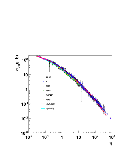
Figure 9: The theoretical prediction for the photoabsorption cross section $\sigma_{\gamma^{*}p}(\eta(W^{2},Q^{2}),\xi)$ for $\xi=130$ compared with the experimental data on DIS.

In fig.9, we show the total cross section,

$$\sigma_{\gamma^{*}p}(W^{2},Q^{2})=\sigma_{\gamma^{*}p}\left(\eta(W^{2},Q^{2}),\frac{m^{2}_{0}}{\Lambda^{2}_{sat}(W^{2})},\xi=\xi_{\rm exp}=130\right)$$ (5.8)

as a function of the low-$x$ scaling variable $\eta(W^{2},Q^{2})$. The upper and the lower theoretical curve in fig.9 refer to the variation of $\sigma^{(\infty)}(W^{2})$ under variation of the energy $W$, i.e. $\sigma(W=275{\rm GeV})\equiv\sigma^{(\infty)}(W^{2}=275^{2}{\rm GeV}^{2})$ and $\sigma(W=10{\rm GeV})\equiv\sigma^{(\infty)}(W^{2}=100{\rm GeV}^{2})$. It is interesting to note that the violation of scaling in $\eta(W^{2},Q^{2})$ of the order of about 10%, as a consequence of the $W$ dependence of the $(q\bar{q})p$ dipole cross section $\sigma^{(\infty)}(W^{2})$, is seen in the experimental data: the high-energy data from ZEUS and H1 lie above the data obtained at lower energies.

Figure 10: The approach to the saturation limit of $F_{2}(\eta(W^{2},Q^{2}),Q^{2})/\sigma_{\gamma p}(W^{2})$ for $\eta(W^{2},Q^{2})\ll 1$.

Figure 10 is relevant for the discussion of the limit of $W^{2}\!\rightarrow\!\infty$ for fixed values of $Q^{2}$ given in Section 2, compare(2.99) and Table 1. In terms of the structure function $F_{2}(x\cong Q^{2}/W^{2},Q^{2})$ the $W^{2}\rightarrow\infty$ limit in (2.99) becomes

$$\lim\limits_{{W^{2}\rightarrow\infty}\atop{Q^{2}{\rm fixed}}}\frac{F_{2}(x\cong Q^{2}/W^{2},Q^{2})}{\sigma_{\gamma p}(W^{2})}=\frac{Q^{2}}{4\pi^{2}\alpha}.$$ (5.9)

Higher energies are required to uniquely experimentally verify the expected saturation property for a larger range of $\eta(W^{2},\,Q^{2})\ll 1$ and fixed values of $Q^{2}$.

Figure 11: The proton structure function $F_{2}(W^{2},Q^{2})$ as a function of $Q^{2}$ for various values of $W$. The theoretical prediction of the CDP is compared with the Caldwell 2 P-fit as a representation of the experimental data.

Figure 12: As in Fig.11, but as a function of $1/W^{2}$ for various values of $Q^{2}\leq 10{\rm GeV}^{2}$.

Figure 13: As in Fig.12, but for $30{\rm GeV}^{2}<Q^{2}<316{\rm GeV}^{2}$.

In figs.11 to 13, we show our predictions from the CDP for the proton structure function $F_{2}(W^{2},Q^{2})$ as a function of $Q^{2}$ for fixed values of $W^{2}$, and as a function of $W^{2}$ for fixed values of $Q^{2}$. For comparison, we also show the results of a very precise fit to the world experimental data for $F_{2}(x,Q^{2})$ for $x<0.025$ (and $Q^{2}>0$) carried out by Caldwell [24]. In particular, we show the results from the so-called 2P-fit that is based on the simple ansatz [24]

$$\sigma_{\gamma^{*}p}=\sigma_{0}\frac{M^{2}}{Q^{2}+M^{2}}\left(\frac{l}{l_{0}}\right)^{\epsilon_{0}+(\epsilon_{1}-\epsilon_{0})\sqrt{\frac{Q^{2}}{Q^{2}+\Lambda^{2}}}}$$ (5.10)

where

$$l=\frac{1}{2x_{bj}M_{p}}.$$ (5.11)

The curves in figs.11 to 13 use the mean values of the six fit parameters $\sigma_{0},M^{2},l_{0},\epsilon_{0},\epsilon_{1}$ and $\Lambda^{2}$ given in Table 5 of ref.[24]. There is acceptable agreement of the predictions of the CDP with the results of the 2P-fit.

In figs.14 and 15, we directly compare the theoretical results for $F_{2}(W^{2},Q^{2})$ from the CDP (shown in figs.11 to 13) with the world experimental data [32]. As expected from figs.11 to 13, there is consistency between the CDP and the experimental data in the full range of $0.036{\rm GeV}^{2}\leq Q^{2}\leq 316{\rm GeV}^{2}$. The theoretical curves are restricted by the condition of $x\cong Q^{2}/W^{2}<0.1$.

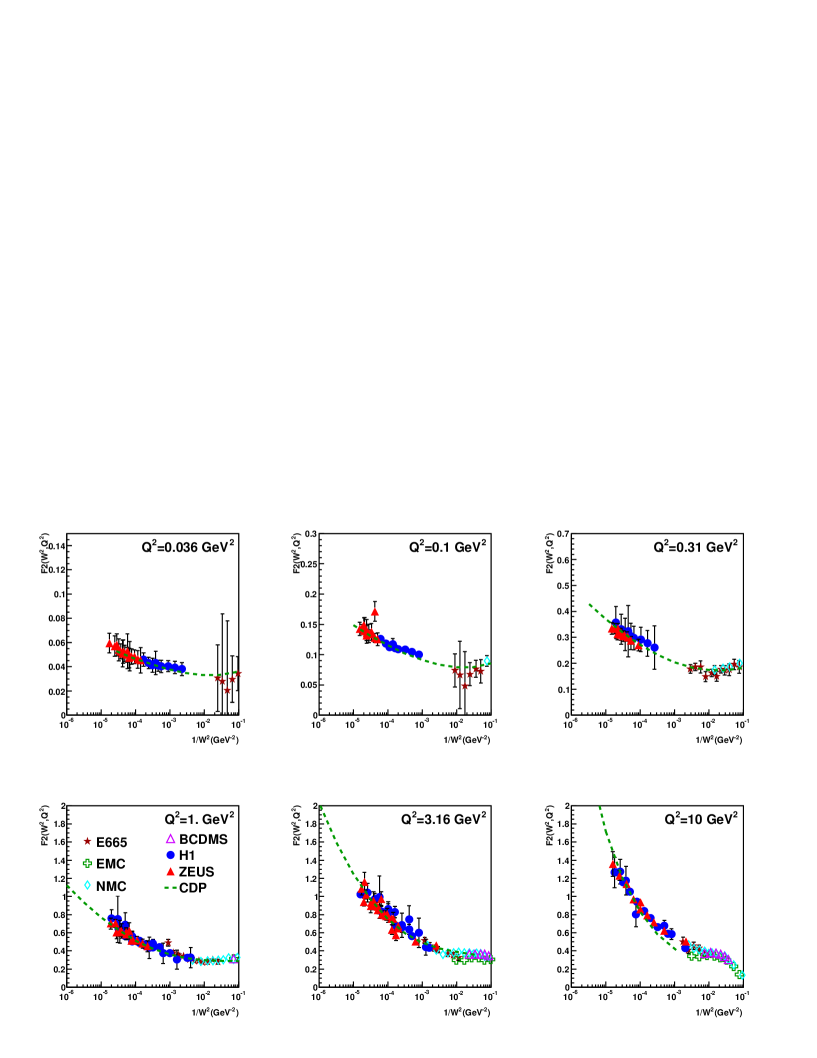
Figure 14: The predictions from the CDP for the structure functionn $F_{2}(W^{2},Q^{2})$ compared with the experimental data for $0.036{\rm GeV}^{2}\leq Q^{2}\leq 10{\rm GeV}^{2}$.

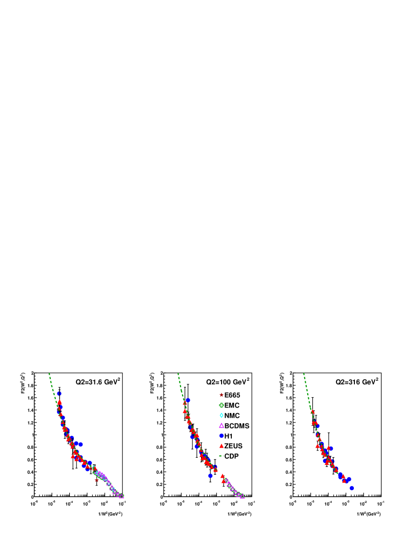
Figure 15: As in fig. 14, but for $31.6{\rm GeV}^{2}\leq Q^{2}\leq 316{\rm GeV}^{2}$.

As noted in the above discussion of the theoretical results in fig.10, experimental data at much higher energies than available at present are needed for a detailed verification of the approach to the saturation limit (5.9). An indication of the proportionality of $F_{2}(x\cong Q^{2}/W^{2},Q^{2})$ to $Q^{2}$ according to (5.9) becomes visible, however, when comparing the experimental data in fig.14 for the very low values of $Q^{2}_{1}=0.036{\rm GeV}^{2}$ and $Q^{2}_{2}=0.1{\rm GeV}^{2}$ with each other. According to the proportionality in (5.9), for sufficiently large $W^{2}$ we have

$$F_{2}(W^{2},Q^{2}_{2}=0.1{\rm GeV}^{2}) = \frac{Q^{2}_{2}}{Q^{2}_{1}}F_{2}(W^{2},Q^{2}_{1}=0.036{\rm GeV}^{2})$$ (5.12)

$$= 2.78F_{2}(W^{2},Q^{2}_{1}=0.036{\rm GeV}^{2}).$$

$\frac{1}{W^{2}}[{\rm GeV}^{-2}]$	$F_{2}(W^{2},Q^{2}_{1}=0.036{\rm GeV}^{2})$	$\frac{Q^{2}_{2}}{Q^{2}_{1}}F_{2}(W^{2},Q^{2}_{1}=0.036{\rm GeV}^{2})$
$2\cdot 10^{-5}$	$\cong 0.055$	0.15
$10^{-4}$	$\cong 0.04$	0.11

• The (approximate) validity of the proportionality (5.12). The results in the second column were read off from fig.14. The predictions from (5.12) in the third column (approximately) agree with the experimental results in fig.14.

The theoretical results for $F_{2}(W^{2},Q^{2}_{2}=0.1{\rm GeV}^{2})$ obtained from (5.12) and shown in Table 3 are consistent with the experimental results in fig.14.

In figs.16 and 17, in addition to the theoretical results in figs.14 and 15, we show the prediction (2.124) of $F_{2}(W^{2})=f_{2}\cdot(W^{2}/1{\rm GeV}^{2})^{0.29}$, where $f_{2}$ is the fitted normalization constant of $f_{2}=0.063$ from (2.125), and $W^{2}\cong Q^{2}/x$. As expected from the analysis in Section 2.7 and fig.4a, there is agreement between theory and experiment for $10{\rm GeV}^{2}\leq Q^{2}\leq 100{\rm GeV}^{2}$ and disagreement for values of $Q^{2}$ outside of this range.

Equation (2.7) may be inverted and read as a prediction for $F_{2}(W^{2}=Q^{2}/x)$ from the pQCD-improved parton picture in terms of a suitable gluon distribution i.e. as a prediction for the flavor-singlet quark distribution, according to

$$F_{2}(W^{2}=\frac{Q^{2}}{x})=\frac{5}{18}x\sum(x,Q^{2})=\frac{(2\rho+1)\sum Q^{2}_{q}}{3\pi}\xi^{C_{2}}_{L}\alpha_{s}(Q^{2})G(x,Q^{2}).$$ (5.13)

In (5.13), the numerical values for the gluon-distribution function have to be inserted, which are obtained by evaluating the right-hand side of the second equality in (2.7). The resulting gluon distributions were shown in fig.7. Since (5.13) coincides with (2.7), the resulting structure function $F_{2}(W^{2},Q^{2})$ is identical to the one given by (2.124) and shown in figs.16 and 17.

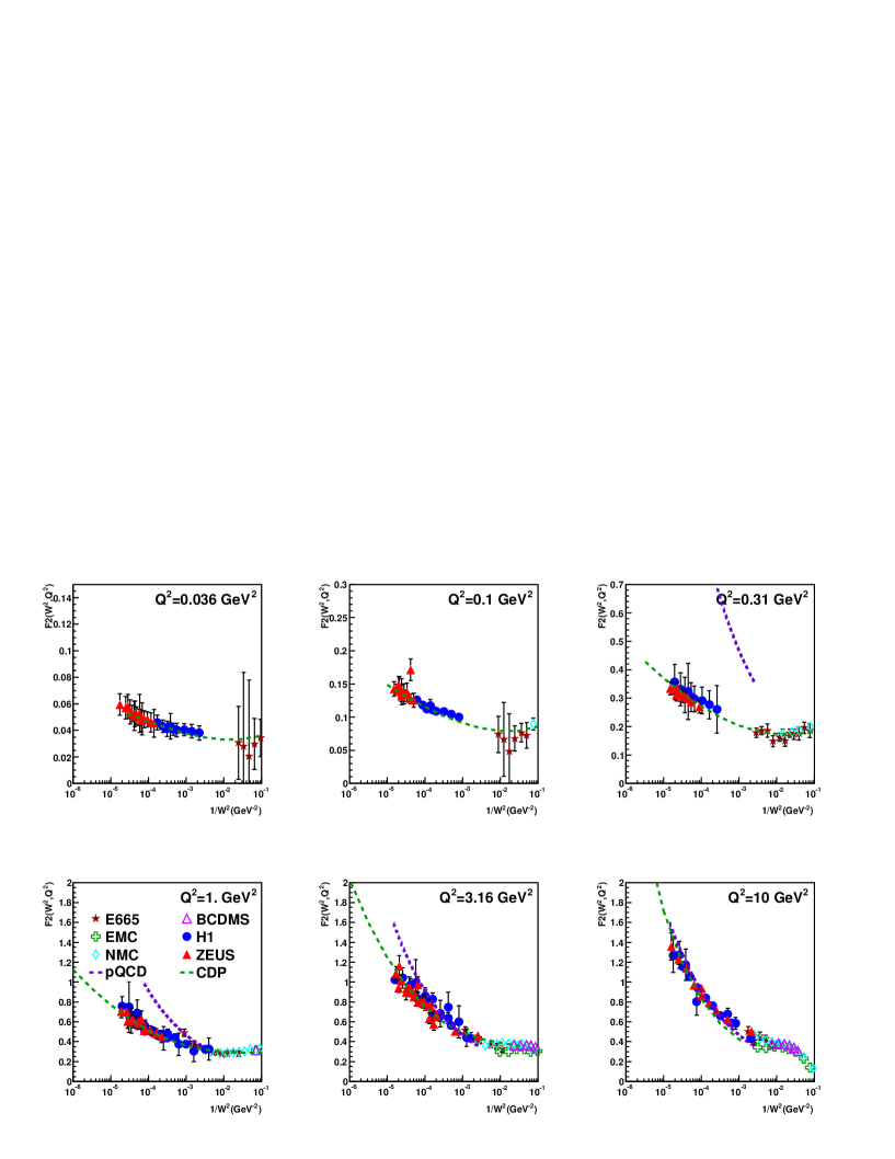
Figure 16: In addition to the prediction from the CDP, also the prediction of $F_{2}(W^{2})=f_{2}\cdot(W^{2}/1{\rm GeV}^{2})^{0.29}$ from (2.124) and (2.125) (valid for $10{\rm GeV}^{2}\leq Q^{2}<100{\rm GeV}^{2}$) for $Q^{2}\leq 10{\rm GeV}^{2}$.

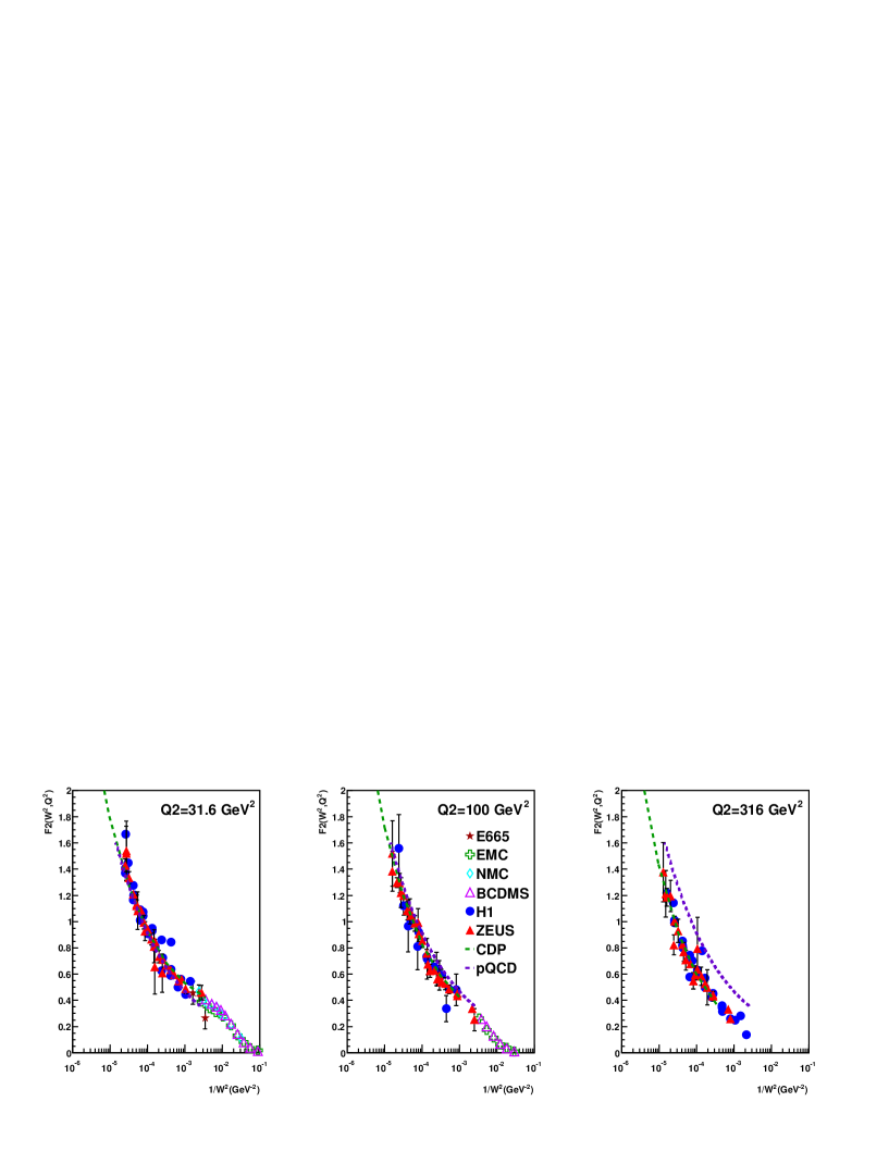
Figure 17: As in fig.16, but for $31.6{\rm GeV}^{2}\leq Q^{2}\leq 316{\rm GeV}^{2}$.

The present interpretation of the results for $F_{2}(W^{2},Q^{2})$ is different, however. The agreement with experiment in figs.16 and 17 shows that a suitable choice of the gluon distribution, compare fig.7, yields agreement with experiment for $F_{2}(W^{2},Q^{2})$ in the relevant range of $10{\rm GeV}^{2}\leq Q^{2}\leq 100{\rm GeV}^{2}$. The results in figs.16 and 17 thus explicitly display the agreement with the pQCD-improved parton picture based on the gluon distribution function of fig.7 in Section 2.7. For the ensuing discussion, we note the proportionality of the gluon distribution function to the saturation scale,

$$\alpha_{s}(Q^{2})G(x,Q^{2})\sim\left(\frac{W^{2}}{1{\rm GeV}^{2}}\right)^{C_{2}=0.29}\sim\Lambda^{2}_{\rm sat}(W^{2})\sigma_{L}^{(\infty)}$$ (5.14)

that follows from comparing (5.13) with the representation of $F_{2}(W^{2},Q^{2})$ in terms of the saturation scale, $\Lambda^{2}_{\rm sat}(W^{2})$, in (2.63) with (2.74) and $\sigma_{L}^{(\infty)}\cong{\rm const.}$ Compare also (2.101) for the approximation of (5.1) by the proportionality to $(W^{2}/1{\rm GeV}^{2})$ used in (5.14).

The pQCD-improved parton picture in (5.13) with the power-like $W^{2}$ dependence (5.14) fails as soon as $\eta(W^{2},Q^{2})<1$, or $Q^{2}<10{\rm GeV}^{2}$, compare fig.16. The saturation behavior of the CDP sets in. For sufficiently large $W^{2}$, at any fixed value of $Q^{2}$, it leads to a logarithmic dependence of $\sigma_{\gamma^{*}p}(W^{2},Q^{2})$, and of $F_{2}(W^{2},Q^{2})$, on the energy $W$, or on $\Lambda^{2}_{\rm sat}(W^{2})$ as given in (2.6), (2.99) and (5.9),

$$F_{2}(W^{2},Q^{2}) \sim Q^{2}\sigma_{L}^{(\infty)}\ln\frac{\Lambda^{2}_{\rm sat}(W^{2})}{Q^{2}+m^{2}_{0}}$$

$$\sim Q^{2}\sigma_{L}^{(\infty)}\ln\left(\frac{\alpha_{s}(Q^{2})G(x,Q^{2})}{\sigma_{L}^{(\infty)}(Q^{2}+m^{2}_{0})}\right),~{}~{}~{}~{}~{}({\rm for}~{}\eta(W^{2},Q^{2})\ll 1).$$

In distinction from the pQCD-improved parton picture in (5.13), for
$\eta(W^{2},Q^{2})<1$, the structure function in (5) depends logarithmically on the gluon distribution function.

The CDP with its $W$-dependent $(q\bar{q})$-dipole-proton cross section is unique in providing a smooth transition from the region of $\eta(W^{2},Q^{2})>1$, with pieceful coexistence between the CDP and the pQCD-improved parton picture, to the saturation region of $\eta(W^{2},Q^{2})<1$, exclusively governed by the CDP. The pQCD-improved parton picture is not allowed to invade the region of $\eta(W^{2},Q^{2})<1$. The suppressed gluon distribution function at $x<10^{-2}$, occasionally with even negative results, from global fits (compare fig.7) is presumably related to the inclusion of experimental data for $F_{2}(x,Q^{2})$ at very low values of $Q^{2}$, where saturation must actually be taken into account, compare (5).

The CDP, in distinction from the discrimination between a soft and a hard Pomeron of the low-$x$ Regge picture [29], only knows of a single Pomeron governing both the regions of $\eta(W^{2},Q^{2})>1$ and of $\eta(W^{2},Q^{2})<1$. The transition from $\eta(W^{2},Q^{2})>1$ to $\eta(W^{2},Q^{2})<1$, or to $W^{2}\rightarrow\infty$ at fixed $Q^{2}$, is not associated with the transition to a (first or second) soft-Pomeron exchange. The transition corresponds to $\Lambda^{2}_{\rm sat}(W^{2})\rightarrow\ln\Lambda^{2}_{\rm sat}(W^{2})$, or equivalently to $\alpha_{s}(Q^{2})G(x,Q^{2})\rightarrow\ln(\alpha_{s}(Q^{2})G(x,Q^{2}))$. The single Pomeron of the CDP has a less strong increase of the corresponding gluon distribution in fig.7 with decreasing $x$, when compared with the hard Pomeron of the Regge fit.

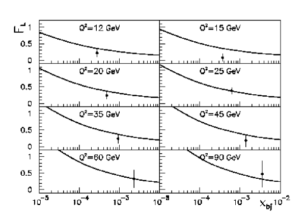
Figure 18: The experimental results on the longitudinal structure function $F_{L}(x,Q^{2})$ from the H1 collaboration[39] compared with the prediction from the CDP.

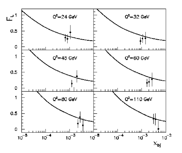
Figure 19: As in fig.18, but showing the experimental results from the ZEUS collaboration[40].

In figs.18 and 19, we show a comparison of our predictions for the longitudinal structure function $F_{L}(x,Q^{2})$ with the experimental data. Since our ansatz for the dipole cross section incorporates transverse-size enhancement, $\rho={\rm const}=4/3$, the theoretical results in figs.18 and 19 agree with the ones in figs. 2 and 3.

6 Conclusion

In the present paper we reexamined and reanalysed DIS at low values of the Bjorken scaling variable $x\cong Q^{2}/W^{2}<0.1$ in terms of the CDP with a $W$-dependent color-dipole cross section. We explicitly showed that all essential features of the experimental data on the longitudinal and the transverse photoabsorption cross section can be understood as a consequence of the color-gauge-invariant $q\bar{q}$-dipole-proton interaction, without relying on any specific parameterization of the dipole-proton cross section.

We also examined the consistency between the description of the experimental data in the CDP and the description in terms of $q\bar{q}$-sea and gluon distributions of the pQCD-improved parton picture within its range of validity.

The resulting $(Q^{2},W^{2})$ plane of DIS at low $x$ consists of only two regions, separated by the line $\eta(W^{2},Q^{2})\cong 1$.

For $\eta(W^{2},Q^{2})\cong Q^{2}/\Lambda^{2}_{\rm sat}(W^{2})\gg 1$ i.e. for sufficiently large $Q^{2}$, color transparency of the color-dipole-proton cross section becomes relevant: the strong destructive interference among different dipole-proton scattering amplitudes originating as a consequence of color-gauge invariance implies a $(q\bar{q})$-proton interaction that vanishes proportional to the transverse dipole size, $\vec{r}^{~{}2}_{\bot}$. The photoabsorption cross section correspondingly behaves as $\Lambda^{2}_{\rm sat}(W^{2})/Q^{2}$, and the proton structure function (for $10{\rm GeV}^{2}\!\!\leq\!\!Q^{2}\!\leq\!100{\rm GeV}^{2}$) as $F_{2}(x,Q^{2})=F_{2}(W^{2}=Q^{2}/x)$.

The experimental data for $\eta(W^{2},Q^{2})>1$ can alternatively be represented in terms of the $(q\bar{q})$-sea-quark and the gluon distribution of the pQCD-improved parton picture. Consistency of the pQCD approach with the CDP requires the gluon distribution function to be proportional to the saturation scale, $\Lambda^{2}_{\rm sat}(W^{2})$, and implies a definite value for the exponent $C_{2}$ in the representation of the saturation scale, $\Lambda^{2}_{\rm sat}(W^{2})\sim(W^{2})^{C_{2}}$. The resulting prediction, $C_{2}\cong 0.27$ to $C_{2}\cong 0.29$, is consistent with the experimental data. The formulation of the CDP in terms of a $W$-dependent ($Q^{2}$-independent) color-dipole-proton cross section is essential to arrive at this conclusion.

With increasing energy, $W$, for any fixed dipole size, $\vec{r}_{\bot}^{~{}2}$, again due to color-gauge invariance, the destructive interference among different amplitudes contributing to the $q\bar{q}$ interaction with the color field of the nucleon dies out and leads to an $\vec{r}^{~{}2}_{\bot}$-independent limit for the $(q\bar{q})$-proton cross section. The $q\bar{q}$-proton cross section “saturates” in this high-energy limit to become identical to a cross section of hadronic size.

The limit of increasingly larger energy, $W$, at fixed dipole size in the photoabsorption process is realized by $W^{2}\rightarrow\infty$ at fixed $Q^{2}$, or $\eta(W^{2},Q^{2})\ll 1$. The photoabsorption cross section increases logarithmically with the energy according to $\ln\Lambda^{2}_{\rm sat}(W^{2})$, and for $W^{2}\rightarrow\infty$ at any fixed value of $Q^{2}$, it reaches the limit of $(Q^{2}=0)$ photoproduction. The pQCD-improved parton picture fails, insofar as the photoabsorption cross section in this limit depends logarithmically on the ($W$-dependent) gluon distribution function.

A concrete parameterization of the dipole cross section is necessary for the interpolation between the regions of $\eta(W^{2},Q^{2})>1$ and $\eta(W^{2},Q^{2})<1$. We refined previous work in several respects, the representation of the longitudinal-to-transverse ratio of the photoabsorption cross section by taking into account the transverse-size enhancement of $q\bar{q}$ fluctuations originating from transversely polarized photons, the extension of the CDP to include the region of $x$ increasing to values close to $x=0.1$, among others. We found agreement with the available DIS data in the full range of $0.036{\rm GeV}^{2}\leq Q^{2}\leq 316{\rm GeV}^{2}$ for $x\leq 0.1$.

Acknowledgement

Useful discussions with Allen Caldwell and Reinhart Kögerler, as well as the help of Prabdeep Kaur for providing plots of experimental data, are gratefully acknowledged.

Appendix A. Derivation of (4.1) and (4.2)

In this Appendix, we derive the photoabsorption cross section in the momentum space (4.1) and (4.2) from the coordinate representation (2.39). We start with the integral representation of the modified Bessel function

$$K_{0}(r^{\prime}_{\perp}Q)={1\over{2\pi}}\int d^{2}\vec{k}_{\perp}^{~{}\prime}{1\over{Q^{2}+\vec{k}^{~{}\prime 2}_{\perp}}}e^{-i\vec{r}^{~{}\prime}_{\bot}\cdot\vec{k}_{\bot}^{~{}\prime}}$$ (A.1)

where

$$r^{\prime}_{\perp}=|\vec{r}^{~{}\prime}_{\bot}|,~{}~{}Q=\sqrt{Q^{2}}.$$ (A.2)

(A.1) can be easily verified from the following equations,

$$\int_{0}^{2\pi}d\theta\exp\left(-iz\cos\theta\right) = 2\pi J_{0}(z),$$ (A.3)

$$\int_{0}^{\infty}dx{x\over{Q^{2}+x^{2}}}J_{0}(r^{\prime}_{\perp}x) = K_{0}(r_{\perp}^{\prime}Q).$$ (A.4)

We compute the following quantity

$$I_{L}(\vec{l}_{\perp}^{~{}\prime 2})\equiv\int d^{2}\vec{r}^{~{}\prime}_{\bot}K^{2}_{0}(r_{\perp}^{\prime}Q)e^{-i\vec{r}^{~{}\prime}_{\bot}\cdot\vec{l}_{\bot}^{~{}\prime}}$$ (A.5)

Inserting (A.1), we find

$$I_{L}(\vec{l}_{\perp}^{~{}\prime 2}) = {1\over{(2\pi)^{2}}}\int d^{2}\vec{r}_{\perp}^{~{}\prime}\int d^{2}\vec{k}^{~{}\prime}_{\perp}$$ (A.6)

$$~{}~{}~{}~{}~{}~{}~{}~{}~{}~{}\int d^{2}\vec{k}_{\perp}^{~{}\prime\prime}{1\over{(Q^{2}+\vec{k}_{\perp}^{~{}\prime 2})(Q^{2}+\vec{k}_{\perp}^{~{}\prime\prime 2})}}e^{-i\vec{r}_{\perp}^{~{}\prime}\cdot(\vec{k}_{\perp}^{~{}\prime}+\vec{k}_{\perp}^{~{}\prime\prime}+\vec{l}_{\perp}^{~{}\prime})}$$

$$= \int d^{2}\vec{k}_{\perp}^{\prime}{1\over{(Q^{2}+\vec{k}_{\perp}^{~{}\prime 2})(Q^{2}+(\vec{k}_{\perp}^{\prime}+\vec{l}_{\perp}^{~{}\prime})^{2})}}$$

$$= \int d\vec{k}^{~{}\prime 2}_{\bot}\int_{0}^{\pi}d\vartheta{1\over{(Q^{2}+\vec{k}_{\perp}^{~{}\prime 2})(Q^{2}+(\vec{k}_{\perp}^{\prime}+\vec{l}_{\perp}^{~{}\prime})^{2})}}$$

where $\vartheta$ is an angle between $\vec{k}_{\perp}^{~{}\prime}$ and $\vec{l}_{\perp}^{\prime}$. Recalling (4.9), we have

$$d\vartheta=-\omega(M^{2},M^{\prime 2},\vec{l}_{\perp}^{~{}\prime 2})dM^{\prime 2}.$$ (A.7)

Inserting (2.44) and (A.6) and using(A.7), the integral in (2.39) becomes

$$\int dr_{\perp}^{\prime 2}K_{0}^{2}(r_{\perp}^{\prime}Q)\sigma_{(q\bar{q})_{L}^{J=1}p}(r_{\perp}^{\prime},W^{2})$$

$$= \int dl_{\perp}^{\prime 2}\bar{\sigma}_{(q\bar{q})_{L}^{J=1}p}(l_{\perp}^{\prime 2},W^{2})\left(I_{L}(0)-I_{L}(l^{\prime 2}_{\perp})\right)$$

$$= \int dl_{\perp}^{\prime 2}\bar{\sigma}_{(q\bar{q})_{L}^{J=1}p}(l_{\perp}^{\prime 2},W^{2})$$

$$\int dM^{2}\int dM^{\prime 2}\omega(M^{2},M^{\prime 2},\vec{l}_{\perp}^{~{}\prime 2})\left({1\over{(Q^{2}+M^{2})^{2}}}-{1\over{(Q^{2}+M^{2})(Q^{2}+M^{\prime 2})}}\right),$$

which leads to (4.1).

The transverse cross section (4.2) is derived in a similar manner. Differentiating (A.1) with respect to $\vec{r}^{~{}\prime}_{\perp}$, one finds

$${{\vec{r}^{~{}\prime}_{\perp}}\over{r_{\perp}^{\prime}}}\sqrt{Q^{2}}K_{1}(r_{\perp}^{\prime}Q)={i\over{2\pi}}\int d^{2}k_{\perp}^{\prime}{{\vec{k}_{\perp}^{\prime}}\over{Q^{2}+\vec{k}_{\perp}^{~{}\prime 2}}}e^{-i\vec{r}^{~{}\prime}_{\perp}\cdot\vec{k}_{\perp}^{~{}\prime}}$$ (A.9)

The integral

$$I_{T}(l_{\perp}^{\prime 2})\equiv\int d^{2}\vec{r}^{~{}\prime}_{\perp}K^{2}_{1}(r_{\perp}^{\prime}Q)e^{-i\vec{r}^{~{}\prime}_{\perp}\cdot\vec{l}_{\bot}^{~{}\prime}}$$ (A.10)

can be evaluated as

$$I_{T}(l_{\perp}^{\prime 2}) = {1\over{(2\pi)^{2}}}\int d^{2}\vec{r}_{\perp}^{~{}\prime}\int d^{2}\vec{k}^{\prime}_{\perp}$$ (A.11)

$$~{}~{}~{}~{}~{}~{}~{}~{}~{}~{}\int d^{2}\vec{k}_{\perp}^{~{}\prime\prime}{{-\vec{k}^{\prime}_{\perp}\cdot\vec{k}_{\perp}^{~{}\prime\prime}}\over{Q^{2}(Q^{2}+\vec{k}_{\perp}^{~{}\prime 2})(Q^{2}+\vec{k}_{\perp}^{~{}\prime\prime 2})}}e^{-i\vec{r}^{~{}\prime}_{\perp}\cdot(\vec{k}_{\perp}^{\prime}+\vec{k}_{\perp}^{~{}\prime\prime}+\vec{l}_{\perp}^{~{}\prime})}$$

$$= {1\over{Q^{2}}}\int d^{2}\vec{k}_{\perp}^{\prime}{{\vec{k}_{\perp}^{\prime}\cdot(\vec{k}_{\perp}^{\prime}+\vec{l}_{\perp}^{~{}\prime})}\over{(Q^{2}+\vec{k}_{\perp}^{~{}\prime 2})(Q^{2}+(\vec{k}_{\perp}^{\prime}+\vec{l}_{\perp}^{~{}\prime})^{2})}}$$

$$= {1\over{Q^{2}}}\int dk_{\perp}^{\prime 2}\int_{0}^{\pi}d\vartheta{{\vec{k}_{\perp}^{\prime}\cdot(\vec{k}_{\perp}^{\prime}+\vec{l}_{\perp}^{~{}\prime})}\over{(Q^{2}+\vec{k}_{\perp}^{\prime 2})(Q^{2}+(\vec{k}_{\perp}^{\prime}+\vec{l}_{\perp}^{~{}\prime})^{2})}}$$

Inserting (2.44) and (A.11), the integral in (2.39) becomes

$$\int dr_{\perp}^{\prime 2}K_{1}^{2}(r_{\perp}^{\prime}Q)\sigma_{(q\bar{q})_{T}^{J=1}p}(r_{\perp}^{\prime},W^{2})$$

$$= \int dl_{\perp}^{\prime 2}\bar{\sigma}_{(q\bar{q})_{T}^{J=1}p}(\vec{l}_{\perp}^{~{}\prime 2},W^{2})\left(I_{T}(0)-I_{T}(\vec{l}^{~{}\prime 2}_{\perp})\right)$$

$$= {1\over{Q^{2}}}\int d\vec{l}_{\perp}^{~{}\prime 2}\bar{\sigma}_{(q\bar{q})_{T}^{J=1}p}(\vec{l}_{\perp}^{~{}\prime 2},W^{2})$$

$$\int dM^{2}\int dM^{\prime 2}\omega(M^{2},M^{\prime 2},\vec{l}_{\perp}^{~{}\prime 2})\left({{M^{2}}\over{(Q^{2}+M^{2})^{2}}}-{{M^{2}+M^{\prime 2}-\vec{l}_{\perp}^{~{}\prime 2}}\over{2(Q^{2}+M^{2})(Q^{2}+M^{\prime 2})}}\right),$$

which leads to (4.2).

Appendix B Correction terms

In this Appendix, we will give the explicit expressions for the correction terms, $\Delta\sigma^{(m^{2}_{0})}_{\gamma^{*}_{L,T}p}(W^{2},Q^{2})$ and $\Delta\sigma^{(m^{2}_{1})}_{\gamma^{*}_{L,T}p}(W^{2},Q^{2})$ in (4.17), which in conjunction with the dominant term guarantee the required bound on $M^{\prime 2}$ that is given by $m^{2}_{0}\leq M^{\prime 2}\leq m^{2}_{1}(W^{2})\equiv m^{2}_{1}$ from (4.7).

With the splitting of the integrand (4.10) as applied to the dominant term, the integrations over $d\vartheta$ in (4.12) and (4.13) yield the following results for the correction terms in (4.14),

$$\Delta\sigma^{(m^{2}_{0})}_{\gamma^{*}_{L}p}(W^{2},Q^{2})+\Delta\sigma^{(m^{2}_{1})}_{\gamma^{*}_{L}p}(W^{2},Q^{2})=-\frac{\alpha R_{e^{+}e^{-}}}{3}\int d\vec{l}^{~{}\prime 2}_{\bot}\bar{\sigma}_{(q\bar{q})^{J=1}_{L}p}(\vec{l}^{~{}\prime 2}_{\bot},W^{2})\cdot$$

$$~{}~{}~{}~{}~{}\left(\int^{(\sqrt{\vec{l}^{~{}\prime 2}_{\bot}}+m_{0})^{2}}_{(\sqrt{\vec{l}^{~{}\prime 2}_{\bot}}-m_{0})^{2}}dM^{2}S_{L,0}(M^{2},\vec{l}^{~{}\prime 2}_{\bot},Q^{2},m^{2}_{0})\right.$$

$$~{}~{}~{}~{}~{}~{}~{}~{}~{}~{}\left.+\int^{m^{2}_{1}}_{(m_{1}-\sqrt{\vec{l}^{~{}\prime 2}_{\bot}})^{2}}dM^{2}S_{L,1}(M^{2},\vec{l}^{~{}\prime 2}_{\bot},Q^{2},m^{2}_{1})\right),$$ (B.1)

and

$$\Delta\sigma^{(m^{2}_{0})}_{\gamma^{*}_{T}p}(W^{2},Q^{2})+\Delta\sigma^{(m^{2}_{1})}_{\gamma^{*}_{T}p}(W^{2},Q^{2})=-\frac{\alpha R_{e^{+}e^{-}}}{6}\int d\vec{l}^{~{}\prime 2}_{\bot}\bar{\sigma}_{(q\bar{q})^{J=1}_{T}p}(\vec{l}^{~{}\prime 2}_{\bot},W^{2})\cdot$$

$$~{}~{}~{}~{}~{}\left(\int^{(\sqrt{\vec{l}^{~{}\prime 2}_{\bot}}+m_{0})^{2}}_{(\sqrt{\vec{l}^{~{}\prime 2}_{\bot}}-m_{0})^{2}}dM^{2}S_{T,0}(M^{2},\vec{l}^{~{}\prime 2}_{\bot},Q^{2},m^{2}_{0})\right.$$

$$~{}~{}~{}~{}~{}~{}~{}~{}~{}~{}\left.+\int^{m^{2}_{1}}_{(m_{1}-\sqrt{\vec{l}^{~{}\prime 2}_{\bot}})^{2}}dM^{2}S_{T,1}(M^{2},\vec{l}^{~{}\prime 2}_{\bot},Q^{2},m^{2}_{1})\right),$$ (B.2)

where

$$S_{L,0}(M^{2},\vec{l}^{~{}\prime 2}_{\bot},Q^{2},m^{2}_{0}) = {{Q^{2}}\over{(Q^{2}+M^{2})^{2}}}{{\pi-\vartheta_{0}(M^{2},\vec{l}^{~{}\prime 2}_{\bot},m_{0}^{2})}\over\pi}$$

$$-{{Q^{2}}\over{(Q^{2}+M^{2})\sqrt{X}}}\left(1-{2\over\pi}{\rm arctan}\sqrt{Y(M^{2},\vec{l}^{~{}\prime 2}_{\bot},Q^{2},m^{2}_{0})}\right)$$

$$S_{L,1}(M^{2},\vec{l}^{~{}\prime 2}_{\bot},Q^{2},m^{2}_{1}) = {{Q^{2}}\over{(Q^{2}+M^{2})^{2}}}{{\vartheta_{1}(M^{2},\vec{l}^{~{}\prime 2}_{\bot},m_{1}^{2})}\over\pi}$$

$$-{{Q^{2}}\over{(Q^{2}+M^{2})\sqrt{X}}}{2\over\pi}{\rm arctan}\sqrt{Y(M^{2},\vec{l}^{~{}\prime 2}_{\bot},Q^{2},m^{2}_{1})}$$

$$S_{T,0}(M^{2},\vec{l}^{~{}\prime 2}_{\bot},Q^{2},m^{2}_{0}) = {{M^{2}-Q^{2}}\over{(Q^{2}+M^{2})^{2}}}{{\pi-\vartheta_{0}(M^{2},\vec{l}^{~{}\prime 2}_{\bot},m_{0}^{2})}\over\pi}$$

$$-{{M^{2}-\vec{l}^{~{}\prime 2}_{\bot}-Q^{2}}\over{(Q^{2}+M^{2})\sqrt{X}}}\left(1-{2\over\pi}{\rm arctan}\sqrt{Y(M^{2},\vec{l}^{~{}\prime 2}_{\bot},Q^{2},m^{2}_{0})}\right)$$

$$S_{T,1}(M^{2},\vec{l}^{~{}\prime 2}_{\bot},Q^{2},m^{2}_{1}) = {{M^{2}-Q^{2}}\over{(Q^{2}+M^{2})^{2}}}{{\vartheta_{1}(M^{2},\vec{l}^{~{}\prime 2}_{\bot},m_{1}^{2})}\over\pi}$$

$$-{{M^{2}-\vec{l}^{~{}\prime 2}_{\bot}-Q^{2}}\over{(Q^{2}+M^{2})\sqrt{X}}}{2\over\pi}{\rm arctan}\sqrt{Y(M^{2},\vec{l}^{~{}\prime 2}_{\bot},Q^{2},m^{2}_{1})}$$

In (Appendix B Correction terms) - (Appendix B Correction terms),

$$\vartheta(M^{2},\vec{l}^{~{}\prime 2}_{\bot},m^{2}_{0,1}) = \arccos\frac{m^{2}_{0,1}-M^{2}-\vec{l}^{~{}\prime 2}_{\bot}}{2M\sqrt{\vec{l}^{~{}\prime 2}_{\bot}}},$$ (B.7)

$$X(M^{2},\vec{l}^{~{}\prime 2}_{\bot},Q^{2}) = (M^{2}-\vec{l}^{~{}\prime 2}_{\bot}+Q^{2})^{2}+4Q^{2}\vec{l}^{~{}\prime 2}_{\bot},$$

$$Y(M^{2},\vec{l}^{~{}\prime 2}_{\bot},Q^{2},m^{2}_{0,1}) = \frac{Q^{2}+(M-\sqrt{\vec{l}^{~{}\prime 2}_{\bot}})^{2}}{Q^{2}+(M+\sqrt{\vec{l}^{~{}\prime 2}_{\bot}})^{2}}\cdot\frac{1-\cos\vartheta(M^{2},\vec{l}^{~{}\prime 2}_{\bot},m^{2}_{0,1})}{1+\cos\vartheta(M^{2},\vec{l}^{~{}\prime 2}_{\bot},m^{2}_{0,1})}$$

$$= -\frac{Q^{2}+(M-\sqrt{\vec{l}^{~{}\prime 2}_{\bot}})^{2}}{Q^{2}+(M+\sqrt{\vec{l}^{~{}\prime 2}_{\bot}})^{2}}\cdot\frac{(\sqrt{\vec{l}^{~{}\prime 2}_{\bot}}+M)^{2}-m^{2}_{0,1}}{(\sqrt{\vec{l}^{~{}\prime 2}_{\bot}}-M)^{2}-m^{2}_{0,1}}>0$$

$$~{}~{}~{}~{}~{}~{}~{}~{}~{}~{}~{}~{}~{}~{}~{}~{}~{}~{}~{}~{}~{}~{}~{}~{}{\rm for}~{}\sqrt{\vec{l}^{~{}\prime 2}_{\bot}}>2m_{0},$$

For photoproduction, $Q^{2}=0$, from (B.2) and (Appendix B Correction terms), (Appendix B Correction terms), we have the simplified expression

$$\Delta\sigma^{(m^{2}_{0})}_{\gamma^{*}_{T}p}(W^{2},Q^{2}=0)+\Delta\sigma^{(m^{2}_{1})}_{\gamma^{*}_{T}p}(W^{2},Q^{2}=0)=$$

$$=-\frac{\alpha R_{e^{+}e^{-}}}{6}\int d\vec{l}^{~{}\prime 2}_{\bot}\bar{\sigma}_{(q\bar{q})^{J=1}_{T}p}(\vec{l}^{~{}\prime 2}_{\bot},W^{2})\cdot$$ (B.8)

$$\cdot\left(\int^{(\sqrt{\vec{l}^{~{}\prime 2}_{\bot}}+m_{0})^{2}}_{(\sqrt{\vec{l}^{~{}\prime 2}_{\bot}}-m_{0})^{2}}{{dM^{2}}\over{M^{2}}}\left({{\pi-\vartheta_{0}(M^{2},\vec{l}^{~{}\prime 2}_{\bot},m_{0}^{2})}\over\pi}\right.\right.$$

$$~{}~{}~{}~{}~{}~{}~{}~{}~{}~{}~{}~{}~{}~{}~{}~{}~{}~{}~{}~{}~{}~{}~{}~{}~{}~{}\left.\left.-{{M^{2}-\vec{l}^{~{}\prime 2}_{\bot}}\over{|M^{2}-\vec{l}^{~{}\prime 2}_{\bot}|}}\left(1-{2\over\pi}{\rm arctan}\sqrt{Y(M^{2},\vec{l}^{~{}\prime 2}_{\bot},Q^{2}=0,m^{2}_{0})}\right)\right)\right.$$

$$\left.+\int^{m^{2}_{1}}_{(m_{1}-\sqrt{\vec{l}^{~{}\prime 2}_{\bot}})^{2}}{{dM^{2}}\over{M^{2}}}\left({{\vartheta_{1}(M^{2},\vec{l}^{~{}\prime 2}_{\bot},m_{1}^{2})}\over\pi}-{2\over\pi}{\rm arctan}\sqrt{Y(M^{2},\vec{l}^{~{}\prime 2}_{\bot},Q^{2}=0,m^{2}_{1})}\right)\right)$$

for $m_{1}>2\sqrt{\vec{l}_{\perp}^{~{}\prime 2}}$.

Specializing the dipole cross section in (B.1) to the ansatz (3.13) and its $J=1$ projections in (3.14), the longitudinal cross section in (B.1) becomes

$$\Delta\sigma^{(m^{2}_{0})}_{\gamma^{*}_{L}p}(W^{2},Q^{2})+\Delta\sigma^{(m^{2}_{1}}_{\gamma^{*}_{L}p}(W^{2},Q^{2})=-\frac{\alpha R_{e^{+}e^{-}}}{4}\frac{\sigma^{(\infty)}}{\pi}\int^{1}_{\frac{2}{3a}}dy\frac{y}{\sqrt{1-y}}$$

$$~{}~{}~{}~{}~{}\left(\int^{(\sqrt{\vec{l}^{~{}\prime 2}_{\bot}}+m_{0})^{2}}_{(\sqrt{\vec{l}^{~{}\prime 2}_{\bot}}-m_{0})^{2}}dM^{2}S_{L,0}(M^{2},\vec{l}^{~{}\prime 2}_{\bot},Q^{2},m^{2}_{0})\right.$$

$$~{}~{}~{}~{}~{}~{}~{}~{}~{}~{}\left.+\int^{m^{2}_{1}}_{(m_{1}-\sqrt{\vec{l}^{~{}\prime 2}_{\bot}})^{2}}dM^{2}S_{L,1}(M^{2},\vec{l}^{~{}\prime 2}_{\bot},Q^{2},m^{2}_{1})\right),$$ (B.9)

while for the transverse cross section, we have

$$\Delta\sigma^{(m^{2}_{0})}_{\gamma^{*}_{T}p}(W^{2},Q^{2})+\Delta\sigma^{(m^{2}_{1}}_{\gamma^{*}_{T}p}(W^{2},Q^{2})=-\frac{\alpha R_{e^{+}e^{-}}}{8}\frac{\sigma^{(\infty)}}{\pi}\int^{1}_{\frac{2}{3a}}dy\frac{(1-\frac{1}{2}y)}{\sqrt{1-y}}$$

$$~{}~{}~{}~{}~{}\left(\int^{(\sqrt{\vec{l}^{~{}\prime 2}_{\bot}}+m_{0})^{2}}_{(\sqrt{\vec{l}^{~{}\prime 2}_{\bot}}-m_{0})^{2}}dM^{2}S_{T,0}(M^{2},\vec{l}^{~{}\prime 2}_{\bot},Q^{2},m^{2}_{0})\right.$$

$$~{}~{}~{}~{}~{}~{}~{}~{}~{}~{}\left.+\int^{m^{2}_{1}}_{(m_{1}-\sqrt{\vec{l}^{~{}\prime 2}_{\bot}})^{2}}dM^{2}S_{T,1}(M^{2},\vec{l}^{~{}\prime 2}_{\bot},Q^{2},m^{2}_{1})\right),$$ (B.10)

$\vec{l}^{~{}\prime 2}_{\bot}$ on the right-hand side in (B.9) and (B.10) is to be replaced by the integration variable $y$,

$$\vec{l}^{~{}\prime 2}_{\bot}=\frac{2\bar{\Lambda}^{~{}2}_{sat}(W^{2})}{3y}$$ (B.11)

For photoproduction, from (B.8), we have

$$\Delta\sigma^{(m^{2}_{0})}_{\gamma^{*}_{T}p}(W^{2},Q^{2}=0)+\Delta\sigma^{(m^{2}_{1}}_{\gamma^{*}_{T}p}(W^{2},Q^{2}=0)=$$ (B.12)

$$=-\frac{\alpha R_{e^{+}e^{-}}}{8}\frac{\sigma^{(\infty)}(W^{2})}{\pi}\int^{1}_{\frac{2}{3a}}dy\frac{1-\frac{1}{2}y}{\sqrt{1-y}}\cdot$$

$$\cdot\left(\int^{(\sqrt{\vec{l}^{~{}\prime 2}_{\bot}}+m_{0})^{2}}_{(\sqrt{\vec{l}^{~{}\prime 2}_{\bot}}-m_{0})^{2}}{{dM^{2}}\over{M^{2}}}\left({{\pi-\vartheta_{0}(M^{2},\vec{l}^{~{}\prime 2}_{\bot},m_{0}^{2})}\over\pi}\right.\right.$$

$$~{}~{}~{}~{}~{}~{}~{}~{}~{}~{}~{}~{}~{}~{}~{}~{}~{}~{}~{}~{}~{}~{}~{}~{}~{}~{}\left.\left.-{{M^{2}-\vec{l}^{~{}\prime 2}_{\bot}}\over{|M^{2}-\vec{l}^{~{}\prime 2}_{\bot}|}}\left(1-{2\over\pi}{\rm arctan}\sqrt{Y(M^{2},\vec{l}^{~{}\prime 2}_{\bot},0,m^{2}_{0})}\right)\right)\right.$$

$$\left.+\int^{m^{2}_{1}}_{(m_{1}-\sqrt{\vec{l}^{~{}\prime 2}_{\bot}})^{2}}{{dM^{2}}\over{M^{2}}}\left({{\vartheta_{1}(M^{2},\vec{l}^{~{}\prime 2}_{\bot},m_{1}^{2})}\over\pi}-{2\over\pi}{\rm arctan}\sqrt{Y(M^{2},\vec{l}^{~{}\prime 2}_{\bot},0,m^{2}_{1})}\right)\right)$$

Appendix C. Derivation of (4.28), (4) and (4)

In this Appendix, we derive the approximate expression for $\sigma^{dom}_{\gamma^{*}_{L/T}p}$ in the large $Q^{2}$ region. we expand the integrand $I_{L/T}(\vec{l}_{\perp}^{~{}\prime 2},M^{2},Q^{2})$ in (4.19) and (4.20) in terms of

$$\hat{x}^{2}={{\vec{l}_{\perp}^{~{}\prime 2}}\over{Q^{2}+m_{0}^{2}}},~{}~{}~{}~{}~{}\hat{y}^{2}={{\vec{l}_{\perp}^{~{}\prime 2}}\over{m_{1}^{2}}},~{}~{}~{}~{}~{}\hat{z}^{2}={{m_{0}^{2}}\over{\vec{l}_{\perp}^{~{}\prime 2}}},$$ (C.1)

all of which are small in the limit $Q^{2}\gg\vec{l}_{\perp}^{~{}\prime 2}\gg 1$. Each term in the integrand becomes

$$-{{Q^{2}}\over{M^{2}+Q^{2}}}\Big{|}_{m_{0}^{2}}^{m_{1}^{2}}={{\hat{x}^{2}}\over{\hat{x}^{2}+\hat{y}^{2}}}+o(\hat{x}^{2}\hat{z}^{2}).$$ (C.2)

$${{Q^{2}}\over{\sqrt{\vec{l}_{\perp}^{~{}\prime 2}(\vec{l}_{\perp}^{~{}\prime 2}+4Q^{2})}}}\ln{{\sqrt{\vec{l}_{\perp}^{~{}\prime 2}(\vec{l}_{\perp}^{~{}\prime 2}+4Q^{2})}\sqrt{X}+\vec{l}_{\perp}^{~{}\prime 2}(3Q^{2}-M^{2}+\vec{l}_{\perp}^{~{}\prime 2})}\over{Q^{2}+M^{2}}}\Bigr{]}\Bigg{|}_{m_{0}^{2}}^{m_{1}^{2}}$$ (C.3)

$$= -{{\hat{x}^{2}}\over{\hat{x}^{2}+\hat{y}^{2}}}+{{\hat{x}^{4}+3\hat{x}^{2}\hat{y}^{2}+6\hat{y}^{4}}\over{6(\hat{x}^{2}+\hat{y}^{2})^{3}}}\hat{x}^{4}+\cdots.$$

$${1\over 2}\ln{{M^{2}+Q^{2}}\over{\sqrt{X}+M^{2}-\vec{l}_{\perp}^{~{}\prime 2}+Q^{2}}}\Big{|}_{m_{0}^{2}}^{m_{1}^{2}}\\ ={{\hat{x}^{2}}\over 2}\Bigl{[}{{\hat{x}^{2}\hat{y}^{2}}\over{(\hat{x}^{2}+\hat{y}^{2})^{2}}}+\cdots\Bigr{]},$$

$$-{{2Q^{2}+\vec{l}_{\perp}^{~{}\prime 2}}\over{2\sqrt{\vec{l}_{\perp}^{~{}\prime 2}(\vec{l}_{\perp}^{~{}\prime 2}+4Q^{2})}}}\ln{{\sqrt{\vec{l}_{\perp}^{~{}\prime 2}(\vec{l}_{\perp}^{~{}\prime 2}+4Q^{2})}\sqrt{X}+\vec{l}_{\perp}^{~{}\prime 2}(3Q^{2}-M^{2}+\vec{l}_{\perp}^{~{}\prime 2})}\over{Q^{2}+M^{2}}}\Bigg{|}_{m_{0}^{2}}^{m_{1}^{2}}$$ (C.4)

$$= {{\hat{x}^{2}}\over{\hat{x}^{2}+\hat{y}^{2}}}+{{2\hat{x}^{4}+3\hat{x}^{2}\hat{y}^{2}-3\hat{y}^{4}}\over{6(\hat{x}^{2}+\hat{y}^{2})^{3}}}\hat{x}^{4}+\cdots$$

Inserting (C.2)-(C.4) into (4.18), we find

$$\sigma_{\gamma^{*}_{L}p}^{dom}(W^{2},Q^{2})={{\alpha R_{e^{+}e^{-}}}\over 3}\int d\vec{l}_{\perp}^{~{}\prime 2}\bar{\sigma}_{(q\bar{q})_{L}^{J=1}p}(\vec{l}_{\perp}^{~{}\prime 2},W^{2})\hat{x}^{2}\Bigl{[}{{\hat{x}^{4}+3\hat{x}^{2}\hat{y}^{2}+6\hat{y}^{4}}\over{6(\hat{x}^{2}+\hat{y}^{2})^{3}}}\hat{x}^{2}+\cdots\Bigr{]},$$ (C.5)

and

$$\sigma_{\gamma^{*}_{T}p}^{dom}(W^{2},Q^{2})={{\alpha R_{e^{+}e^{-}}}\over 3}\int d\vec{l}_{\perp}^{~{}\prime 2}\bar{\sigma}_{(q\bar{q})_{L}^{J=1}p}(\vec{l}_{\perp}^{~{}\prime 2},W^{2})\hat{x}^{2}\Bigl{[}{{\hat{x}^{2}+3\hat{y}^{2}}\over{3(\hat{x}^{2}+\hat{y}^{2})^{3}}}\hat{x}^{4}+\cdots\Bigr{]}.$$ (C.6)

Recalling

$${{\hat{x}^{2}}\over{\hat{y}^{2}}}={\xi\over\eta},$$ (C.7)

and introducing the integration variable $y$ defined by (4.21),

$$\hat{x}^{2}={2\over{3\eta y}},$$ (C.8)

we find

$$\sigma_{\gamma^{*}_{L}p}^{dom}(W^{2},Q^{2}) = {{\alpha R_{e^{+}e^{-}}}\over{24}}\Bigl{(}{{\sigma^{(\infty)}(W^{2})}\over\pi}\Bigr{)}\int^{1}_{2/(3a)}dy{y\over{\sqrt{1-y}}}\hat{x}^{2}G_{L}({\xi\over{\eta(W^{2},Q^{2})}})$$ (C.9)

$$= {{\alpha R_{e^{+}e^{-}}}\over{18}}\Bigl{(}{{\sigma^{(\infty)}(W^{2})}\over\pi}\Bigr{)}{1\over\eta(W^{2},Q^{2})}AG_{L}({\xi\over{\eta(W^{2},Q^{2})}}),$$

and

$$\sigma_{\gamma^{*}_{T}p}^{dom}(W^{2},Q^{2}) = {{\alpha R_{e^{+}e^{-}}}\over{12}}\Bigl{(}{{\sigma^{(\infty)}(W^{2})}\over\pi}\Bigr{)}\int^{1}_{2/(3a)}d\hat{y}{{1-\hat{y}/2}\over{\sqrt{1-\hat{y}}}}\hat{x}^{2}G_{T}({\xi\over{\eta(W^{2},Q^{2})}})$$ (C.10)

$$= {{\alpha R_{e^{+}e^{-}}}\over{18}}\Bigl{(}{{\sigma^{(\infty)}(W^{2})}\over\pi}\Bigr{)}{1\over\eta(W^{2},Q^{2})}$$

$$~{}~{}~{}~{}~{}~{}~{}\times\Bigl{[}\log{{1+A}\over{1-A}}-A\bigr{]}G_{T}({\xi\over{\eta(W^{2},Q^{2})}}).$$

Here

$$A\equiv\sqrt{1-{2\over{3a}}}=0.951~{}~{}~{}~{}{\rm for}~{}~{}a=7$$ (C.11)

and the functions $G_{L}({\xi\over{\eta(W^{2},Q^{2})}})$ and $G_{T}({\xi\over{\eta(W^{2},Q^{2})}})$ are defined by (4) and (4). Noting that $A\sim 1$ and

$$\ln{{1+A}\over{1-A}}-A=2A\rho(\epsilon={1\over{6a}})\sim 2\rho(\epsilon={1\over{6a}})$$ (C.12)

we reach the approximate expression for the dominant parts given in (4.28).

References

- [1] J.J. Sakurai and D. Schildknecht, Phys. Lett. 40B, 121 (1972); B. Gorczyca, D. Schildknecht, Phys. Lett. 47B, 71 (1973).
-
[2]
V.N. Gribov, Soviet Phys. JETP 30, 709 (1970);
K. Fujikawa, Phys. Rev. D4, 2794 (1971). - [3] H. Fraas, B.J. Read and D. Schildknecht, Nucl. Phys. B86, 346 (1975); R. Devenish and D. Schildknecht, Phys. Rev. D19, 93 (1976).
- [4] D. Schildknecht, Acta Physica Polonica B37, 595 (2006), [arXiv:hep-ph/0511090].
- [5] N.N. Nikolaev, B.G. Zakharov, Z. Phys. C49, 607 (1991).
- [6] G. Cvetic, D. Schildknecht, A. Shoshi, Eur. Phys. J C13, 301 (2000).
- [7] F.E. Low, Phys. Rev. D12, 163 (1975); S. Nussinov, Phys. Rev. Lett. 34, 1286 (1975); Phys. Rev. D14, 246 (1976); J. Gunion, D. Soper, Phys. Rev. D15, 2617 (1977).
- [8] R. Devenish and A. Cooper-Sarker, Deep Inelastic Scattering, Oxford University Press, 2004.
- [9] H1 Collaboration, T. Ahmed et al., Nucl. Phys. B429, 477 (1994); ZEUS Collaboration, M. Derrick et al., Phys. Lett. B315, 481 (1993); Durham Data Base, http://durpdg.dur.ac.uk/HEPDATA/REAC
- [10] M. Kuroda and D. Schildknecht, Phys. Lett. B670, 129 (2008).
- [11] D. Schildknecht, Contribution to Diffraction 2000, Cetraro, Italy, September 2-7, 2000, Nucl. Phys. B, Proc. Supplement 99 (2001) 121; D. Schildknecht, B. Surrow, M. Tentyukov, Phys. Lett. B499, 116 (2001); G. Cvetic, D. Schildknecht, B. Surrow, M. Tentyukov, EPJC 20, 77 (2001)
-
[12]
L.N. Lipatov, Sov. J. Nucl. Phys. 20 (1975) 95,
V.N. Gribov and L.N. Lipatov, Sov. J. Nucl. Phys. 15 (1972) 438,
G. Altarelli and G. Parisi, Nucl. Phys. B126 (1977) 298;
Yu. L. Dokshitzer, Sov. Phys. JETP 46 (1977) 641. - [13] J.D. Bjorken, J. Kogut, D.E. Soper, Phys. Rev. D3,1382 (1971).
- [14] J.R. Forshaw, G. Kerley, G. Shaw, Phys. Rev. D60, 074012 (1999).
-
[15]
C. Ewerz and O. Nachtmann, Annals of Phys. 322, 1635 (2007); 322, 1670 (2007);
C. Ewerz, A.v. Manteuffel, O. Nachtmann, arXiv:1101.028 [hep-ph]. - [16] M. Kuroda and D. Schildknecht, Phys. Rev. D66, 094005 (2002); Phys. Rev. D67, 094008 (2003).
- [17] I.S. Gradshteyn and I.M. Ryzhik, Academic Press, New York and London (1965) p. 693 formula 6.576-4.
- [18] T. Nieh, Phys. Rev. D1, 3161 (1970); L. Stodolsky, Phys. Rev. Lett. 18, 135 (1967); B.L. Joffe, Phys. Lett. 30 B, 123 (1969).
- [19] C. Bilchak, D. Schildknecht, Phys. Lett. B233, 461 (1989).
- [20] K. Golec-Biernat and A.M. Stasto, arXiv:0905.132 [hep-ph]
- [21] D. Schildknecht, Contribution to DIS 2001, The 9th International Workshop on Deep Inelastic Scattering, Bologna, Italy, 2001, G. Brassi et al. (Eds.), World Scientific, Singapore, 2002, p. 798; D. Schildknecht, B. Surrow and M. Tentyukov, Mod. Phys. Lett. A16 (2001) 1829.
- [22] A.M. Stasto, K. Golec-Biernat, J. Kwiecinski, Phys. Rev. Lett. 86, 596 (2001).
- [23] D. Schildknecht and F. Steiner, Phys. Lett. B56, 36 (1975).
- [24] A. Caldwell, arXiv:0802.0769
- [25] D. Schildknecht, arXiv:1104.0850 [hep-ph]
-
[26]
A.D. Martin, R.G. Roberts and W.J. Stirling, Phys. Rev. D37, (1988) 1161;
A.M. Cooper-Sarkar et al., Z. Phys. C39 (1988) 281. - [27] K. Prytz, Phys. Lett. B311 (1993) 286.
-
[28]
K. Adel, F. Barreiro, F.J. Yndurain, Nucl. Phys. B495 (1997) 221;
F.J. Yndurain, The Theory of Quark and Gluon Interactions (Springer 1999), p.157. - [29] A. Donnachie and P.V. Landshoff, Phys. Lett. B533 (2002) 277, arXiv:hep-ph/0111427; Acta Physica Polonica B34 (2003) 2989, arXiv:hep-ph/0305171.
- [30] M. Kuroda and D. Schildknecht, Phys. Lett. B618 (2005) 84.
- [31] M. Glück, E. Reya, A. Vogt, Z. Phys. C67 (1994) 433; Eur. Phys. J. C5 (1998) 461
- [32] Durham Data Base, http://durpdg.dur.ac.uk/HEPDATA/PDF
- [33] CTEQ Collaboration: J. Pumplin et al., JHEP 0207 (2002) 012.
- [34] A.D. Martin et al., Eur. Phys. J. C18 (2000) 117.
-
[35]
E.A. Kuraev, L.N. Lipatov and V.S. Fadin, Sov. Phys. JETP 44 (1976) 443;
Ya.Ya. Balitskii, L.N. Lipatov, Sov. J. Nucl. Phys. 28 (1978) 822. -
[36]
A.DeRujula et al., Phys. Rev. D10 (1974) 1649;
R.D. Ball and S. Forte, Phys. Lett. B (1994) 77. - [37] N.N. Nikolaev, B.G. Zakharov, Z. Phys. C64 (1994) 631.
- [38] F. Caola and S. Forte, arXiv:0802.187802 [hep-ph], Phys. Rev. Letters 101 (2008) 022001.
- [39] H1 Collaboration, F.D. Aaron et al., Phys. Lett. B665 (2008) 139.
- [40] ZEUS Collaboration, S. Chekanov et al., Phys. Lett. B682(2009) 8.