The observable prestellar phase of the IMF

Abstract

The observed similarities between the mass function of prestellar cores (CMF) and the stellar initial mass function (IMF) have led to the suggestion that the IMF is already largely determined in the gas phase. However, theoretical arguments show that the CMF may differ significantly from the IMF. In this Letter, we study the relation between the CMF and the IMF, as predicted by the IMF model of Padoan and Nordlund. We show that 1) the observed mass of prestellar cores is on average a few times smaller than that of the stellar systems they generate; 2) the CMF rises monotonically with decreasing mass, with a noticeable change in slope at approximately 3-5 M_⊙, depending on mean density; 3) the selection of cores with masses larger than half their Bonnor-Ebert mass yields a CMF approximately consistent with the system IMF, rescaled in mass by the same factor as our model IMF, and therefore suitable to estimate the local efficiency of star formation, and to study the dependence of the IMF peak on cloud properties; 4) only one in five pre-brown-dwarf core candidates is a true progenitor to a brown dwarf.

1. Introduction

Molecular clouds (MCs) undergo a highly non-linear fragmentation process, even prior to the emergence of young stars, or in regions with no apparent star formation. The fundamental reason for their fragmentation is the presence of supersonic turbulence that originates at large scales from various sources, such as supernovae, spiral-arm shocks, or magneto-rotational instability. The formation of dense filaments and cores is the natural evolution of the intersection of randomly driven shocks in the turbulent flow. Even without self-gravity, turbulence simulations with the same rms Mach numbers as MCs generate density contrasts of many orders of magnitude, with characteristic size and density of both filaments and cores as observed in MCs (Arzoumanian et al., 2011). Because all stars are born in MCs, and specifically from dense cores found predominantly within the densest filaments (e.g. André et al., 2010; Arzoumanian et al., 2011), the fragmentation by the turbulence must control the early phases of the star formation process. It may also control its global properties, such as the star formation rate (Krumholz & McKee, 2005; Padoan & Nordlund, 2011) and the mass distribution of stars (Padoan & Nordlund, 2002; Hennebelle & Chabrier, 2008), but other processes (e.g. stellar jets and outflows, disk fragmentation, competitive accretion, ambipolar drift) can also affect the mass and formation rate of stars (e.g. Adams & Fatuzzo, 1996; Bonnell et al., 2001).

Most (sub-)mm or extinction surveys of star-forming regions have resulted in prestellar core mass functions (CMFs) interpreted to be consistent with the stellar IMF (Motte et al., 1998; Testi & Sargent, 1998; Johnstone et al., 2000, 2001; Motte et al., 2001; Onishi et al., 2002; Johnstone et al., 2006; Stanke et al., 2006; André et al., 2007; Enoch et al., 2007, 2008; Belloche et al., 2011). A few studies have also claimed the detection of a CMF peak, which has been interpreted as a scaled progenitor of the stellar IMF peak, with the scaling mass factor giving the local efficiency of star formation (Alves et al., 2007; Nutter & Ward-Thompson, 2007; Rathborne et al., 2009; André et al., 2010; Könyves et al., 2010). However, the peak of the CMF is quite close to the estimated completeness limits of the surveys, which depends also on the core shape and selection method (e.g. Kainulainen et al., 2009; Pineda et al., 2009).

Simple theoretical considerations show that a one-to-one relation between the mass of observed prestellar cores and that of stars is unlikely. Prestellar cores must grow for some time before they can collapse and form stars. When a core is observed it is unlikely to have just reached its final mass. Furthermore, the largest observable mass of a core may be even lower than the full prestellar mass involved. Once a core mass grows beyond its Bonnor-Ebert (BE) mass (Bonnor, 1956; Ebert, 1957), the core rapidly collapses within about a free-fall time, but the accretion flow that was assembling that core is likely to still be active, and to continue to bring additional mass to the new protostar. The prestellar core as such is gone, but the prestellar mass feeding the new protostar may keep coming. Note that this process is essentially inertial, and therefore distinctly different from competitive accretion, which assumes the flow is caused by gravitation forces.

Clark et al. (2007) have stressed a timescale problem in relating the CMF to the stellar IMF: if cores of different masses are assumed to all contain one BE mass, small cores must be denser and free-fall more rapidly than larger ones. If the CMF is stationary in time, the corresponding stellar IMF should then be steeper than the CMF. However, the observations do not show a strong correlation between core mass and density, so this timescale issue may not be the main problem in deriving the IMF from the CMF. In this Letter, we study the relation between the CMF and the stellar IMF based on our IMF model (Padoan & Nordlund, 2002).

2. Random realizations of the IMF model

The IMF model by Padoan & Nordlund (2002) (PN02 hereafter) predicts the mass distribution of gravitationally unstable cores generated by a turbulent flow. The mass of a core is the total mass, $m_{\rm accr}$, the turbulent flow would assemble locally, irrespective of when the core should collapse and cease to appear as prestellar. In PN02, the mass distribution of all cores (unstable or not) is a power law with slope $x=3/(4-b)$, where $b$ is the slope of the velocity power spectrum of the turbulent flow, $E(k)\sim k^{-b}$. The Salpeter slope, $x=1.35$, is thus recovered if $b=1.78$, consistent with power spectra derived from the largest simulations of supersonic and super-Alfvénic turbulence and from observations (e.g. Padoan et al., 2006, 2009). Unstable cores are then selected as those more massive than their BE mass, assuming all cores have the same temperature, while their external density (the local postshock density) follows the Log-Normal pdf of supersonic turbulent flows. Most of the massive cores contain more than one BE mass, so the IMF above approximately one solar mass is predicted to be a power law with slope close to Salpeter’s. Smaller cores are usually less massive than their BE mass, so the IMF is expected to peak at a fraction of a solar mass, and to decline towards smaller masses.

This assumes that the actual stellar mass is $m_{\star}=\epsilon\,m_{\rm accr}$, and the local efficiency, $\epsilon$, is approximately independent of mass. In observational studies, the local efficiency, $\epsilon_{\rm core}$, is instead defined as the ratio of the resulting stellar mass, $m_{\star}$, and the current mass of prestellar cores, $m$, so $\epsilon_{\rm core}=m_{\star}/m$. It follows that the ratio of the total core mass predicted by the model and the current core mass can be expressed as the ratio between our theoretical local efficiency and the observational one, $m_{\rm accr}/m=\epsilon_{\rm core}/\epsilon$, and thus $\epsilon_{\rm core}/\epsilon\geq 1$.

To create a population of observable prestellar cores consistent with the IMF model, we first generate random values of total core masses, $m_{\rm accr}$, following the predicted power law distribution with slope $x=1.35$. We then generate a random value of external density for each core, according to the Log-Normal gas density distribution of the turbulent flow, converted to mass fraction,

$$p(\tilde{\rho})d\tilde{\rho}\propto{\rm exp}\left[-\frac{({\rm ln}\tilde{\rho}+\sigma^{2}/2)^{2}}{2\,\sigma^{2}}\right]d\tilde{\rho},\vspace{0.2cm}$$ (1)

where $\tilde{\rho}$ is the core external density in units of the cloud mean density, $\tilde{\rho}=\rho/\rho_{0}$, and the standard deviation, $\sigma$, of the logarithmic density field is

$$\sigma^{2}={\rm ln}\left[1+\left(\frac{{\cal M}_{\rm S,0}}{2}\right)^{2}(1+\beta^{-1})^{-1}\right],$$ (2)

where ${\cal M}_{\rm S,0}$ is the rms sonic Mach number, ${\cal M}_{\rm S,0}=v_{0}/c_{\rm S,0}$, with $v_{0}$ the three-dimensional rms velocity and $c_{\rm S,0}$ the isothermal sound speed corresponding to the mean temperature $T_{0}$, and $\beta$ is a characteristic ratio of gas to magnetic pressure in the postshock gas (see Padoan & Nordlund, 2011, eqs. 16, 17, 18, 27 and 28). The corresponding standard deviation of the linear density field, $\sigma_{\tilde{\rho}}$, is given by

$$\sigma_{\tilde{\rho}}=(1+\beta^{-1})^{-1/2}{\cal M}_{\rm S,0}/2.$$ (3)

Finally, we associate a random age to each core, assuming for simplicity that the star formation rate (SFR) is uniform over time and independent of core mass.

In order to relate the PN02 model to observations of prestellar cores (cores without a detectable embedded protostar), we also need to account for the time evolution of cores, and define when, during its growth, a core would be observed as prestellar. In PN02, cores are assumed to be chunks of dense postshock filaments (or sheets), with size equal to the postshock thickness, $\lambda$, and mass

$$m_{\rm accr}=(4/3)\pi\rho(\lambda/2)^{3},$$ (4)

where $\rho$ is the postshock density. Assuming that a compression from the scale $\ell$ has a shock velocity that follows the second order velocity structure function of the turbulent flow, $v\sim\ell^{a}$ (with $a=(b-1)/2$), the compression lasts for an accretion time given by

$$t_{\rm accr}=\ell/v=t_{0}(\ell/L_{0})^{1-a},$$ (5)

where $t_{0}$ is the cloud crossing time, defined as the ratio of cloud size, $L_{0}$, and rms velocity, $v_{0}$, $t_{0}=L_{0}/v_{0}$. Assuming that the postshock thickness, $\lambda$, grows linearly with time, we can then model the mass evolution of a prestellar core, up to the time $t=t_{\rm accr}$, when the total core mass, $m_{\rm accr}$, is reached, with the simple law

$$m(t)/m_{\rm accr}=(t/t_{\rm accr})^{3},$$ (6)

which shows that cores must spend a significant fraction of their lifetime at a mass significantly lower than their final mass, and therefore the relation between the masses of prestellar cores and stars cannot be trivial.

In order to express $t_{\rm accr}$ and $m$ as a function of $m_{\rm accr}$, instead of $\ell$, we can relate $m_{\rm accr}$ and $\ell$ using equation (4) with the shock jump conditions, $\rho=\rho_{0}{\cal M}_{\rm A,\ell}$ and $\lambda=\ell/{\cal M}_{\rm A,\ell}$, assuming that the shock Alfvénic Mach number scales like the shock velocity, ${\cal M}_{\rm A,\ell}\sim v\sim\ell^{a}$, and with the effective rms Alfvénic Mach number expression of Padoan & Nordlund (2011) (equations (13) and (14)), ${\cal M}_{\rm A,0}=\sigma_{\tilde{\rho}}^{2}$. We then obtain the following expression for $t_{\rm accr}$ expressed as a function of $m_{\rm accr}$

$$t_{\rm accr}=t_{0}\,\sigma_{\tilde{\rho}}^{{4-4a\over 3-2a}}\left(m_{\rm accr}\over m_{0}\right)^{1-a\over(3-2a)}.$$ (7)

We assume that cores that do not reach their BE mass are seen only during their formation time, $t_{\rm accr}$, while those growing past their BE mass continue to be observed as prestellar for one free-fall time, reaching a maximum prestellar mass, $m_{\rm max}$, given by

$${m_{\rm max}\over m_{\rm accr}}=\left({t_{\rm BE}+t_{\rm ff}}\over t_{\rm accr}\right)^{3},$$ (8)

where $t_{\rm BE}$ is the time when cores reach their BE mass,

$$t_{\rm BE}=t_{\rm accr}\left(m_{\rm accr}\over m_{\rm BE}\right)^{-1/3},$$ (9)

and the BE mass (Bonnor, 1956; Ebert, 1957) is

$$m_{\rm BE}=1.182\,c_{\rm S}^{3}\,/(G^{3/2}\rho^{1/2}),$$ (10)

where $c_{\rm S}$ is the isothermal sound speed in the cores, corresponding to the mean core temperature $T$, $\rho$ the postshock density (assumed to be the external density of the BE sphere), $G$ the gravitational constant, and $t_{\rm ff}$ is the free-fall time, $t_{\rm ff}=(3\pi/(32G\rho))^{1/2}$. The value of $m_{\rm max}$ may be larger than $m_{\rm accr}$ (if $t_{\rm BE}+t_{\rm ff}>t_{\rm accr}$), and therefore the final (observable) mass of a prestellar core as such is

$$m_{\rm f}={\rm min}[m_{\rm accr},m_{\rm max}].$$ (11)

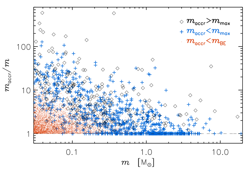
Figure 1.— Ratio of the total core mass and the current core mass, $m$. Dots are for cores that will never collapse into stars, plus symbols for cores that form stars and can reach $m_{\rm accr}$ while prestellar, $m_{\rm f}=m_{\rm accr}<m_{\rm max}$, and diamond symbols for those that form stars but do not reach the mass $m_{\rm accr}$ while prestellar, $m_{\rm f}=m_{\rm max}<m_{\rm accr}$.

3. Results

We show results for a model with characteristic molecular cloud (MC) parameters, $T_{0}=10$ K, $T=7$ K (the core mean temperature), $L_{0}=10$ pc, $\rho_{0}=2\times 10^{-21}$ g/cm³, ${\cal M}_{\rm S,0}=25$, $\beta=0.4$. The total MC mass is then $m_{0}=1.1\times 10^{5}$ M_⊙, and its three-dimensional rms velocity $v_{0}=4.9$ km/s. We consider the simple case of a constant SFR for a time equal to the cloud crossing time, $t_{0}=L_{0}/v_{0}=1.9$ Myr, and study the prestellar core population at a time $t=t_{0}$, assuming that prestellar cores are detected above a minimum surface density of $N_{\rm det}=10^{21}$ cm^-2, corresponding to the Herschel 5-$\sigma$ detection limit due to cirrus noise in Aquila (André et al., 2010; Könyves et al., 2010). We generate a random distribution of total core masses, $m_{\rm accr}$, with probability following a power law with slope $x=1.35$, with a minimum mass of 0.01 M_⊙. The total mass in the cores is $0.26m_{0}$, while the total mass of those that collapse into stars gives a final star formation efficiency of SFE_f=0.05. At the time we study the core population, $t=t_{0}$, the total mass in stars (defined as all the cores that have reached their total mass, $m_{\rm accr}$) is such that SFE$(t_{0})=0.02$, which is a reasonable value for MCs (e.g. Evans et al., 2009). The core formation efficiency at $t=t_{0}$ is CFE$(t_{0})$=0.01, also consistent with observations (e.g. Enoch et al., 2007).

Figure 2.— Histograms of the ratio $m_{\rm accr}/m$ shown in Figure 1. The solid line is the histogram for all cores with mass $m>0.1$ M_⊙, yielding a mean value of $\langle m_{\rm accr}/m\rangle=5.0$. The dashed line in Figure 2 is the histogram including only core masses above half their BE mass, $m>m_{\rm BE}/2$, yielding a mean value of $\langle m_{\rm accr}/m\rangle=2.6$.

Figure 1 shows the ratio between the total core mass and its current mass at time $t=t_{0}$, $m_{\rm accr}/m=\epsilon_{\rm core}/\epsilon$. The plot shows that prestellar cores may have a mass significantly smaller than the mass of the stellar system they will form, assuming reasonable values of $\epsilon$, which means that $\epsilon_{\rm core}>1$, contrary to the usual assumption of observational studies. Observed prestellar cores with masses between 0.1 and 1.0 M_⊙, for example, may be on their way to form stellar systems with masses 10 times larger.

The relation between current core mass and total core mass is quantified by the histograms of the ratio $m_{\rm accr}/m$, shown in Figure 2. The solid line is the histogram for all prestellar cores with mass $m>0.1$ M_⊙, showing a broad distribution, with a mean value of $\langle m_{\rm accr}/m\rangle=5.0$. Cores that will never grow above their BE mass to form stars ($m_{\rm accr}<m_{\rm BE}$) are shown as dots in Figure 1. These cores are not included in the histogram, but they certainly contaminate observational samples.

The dashed line in Figure 2 is the histogram including only core masses above half their BE mass, $m>m_{\rm BE}/2$. These cores are somewhat closer to their corresponding total core masses, with an average ratio of $\langle m_{\rm accr}/m\rangle=2.6$. The ratio of the peak of the stellar IMF from our model (see Figure 4 below) and the peak of the multiple system IMF of Chabrier (2005) is approximately 2.1, corresponding to $\epsilon\approx 0.48$. With this value of the theoretical local efficiency of star formation, the average ratio between the actual mass of stellar systems, $m_{\star}$, and the current mass of cores, $m$, would be $\epsilon_{\rm core}=\epsilon\langle m_{\rm accr}/m\rangle=2.4$ for prestellar cores with $m>0.1$ M_⊙, and $\epsilon_{\rm core}\approx 1.2$ for the core subsample with $m>m_{\rm BE}/2$.

Figure 3 shows the ratio of the current core mass to its BE mass, at $t=t_{0}$. It shows that a significant fraction of the cores with $m>0.1$ M_⊙ may be found to have a mass larger than their BE mass. It also shows that the selection of cores with mass $m>m_{\rm BE}/2$ allows partial decontamination from cores that will never collapse into stars, while still providing a large enough core subsample to allow a meaningful estimation of the CMF. This strategy is already being implemented in the analysis of observational surveys (e.g. Könyves et al., 2010). The solid line in Figure 3 gives the ratio between the number of non-prestellar cores and that of true prestellar cores (computed from five different realizations of the same model), as a function of core mass, for cores with mass $m>m_{\rm BE}/2$. Around 1 M_⊙, only 16% of these cores are not prestellar, while that fraction grows to 35% around 0.1 M_⊙.

Smaller cores that may be progenitors of brown dwarfs can barely exceed their BE mass (towards the end of their lifetime). Only one in five of the selected pre-brown-dwarf core candidates with mass $m_{\rm BE}/2<m<0.15$ M_⊙ (assuming $\epsilon\approx 0.48$) is a true pre-brown-dwarf core. Half of them are growing progenitors of higher mass stars, and one third are non-prestellar cores. Distinguishing true pre-brown-dwarf cores or non-prestellar cores in observational surveys is a difficult task that may require the characterization of such cores using synthetic observations of turbulence simulations.

Figure 3.— Ratio of current core mass to BE mass, plotted versus the current core mass. The solid line shows the ratio between the number of cores that will never collapse and form stellar systems and that of true prestellar cores, after selecting cores with $m>m_{\rm BE}/2$.

The CMF at the time $t=t_{0}$ is shown in Figure 4 by the black histogram (and by the continuous red line for the average of five different realizations of the same model). The CMF seems to change its slope at two mass values, $m_{1}\approx 0.5$ M_⊙ (approximately the peak of the model IMF) and $m_{2}\approx 4$ M_⊙. For masses above $m_{2}$, the slope is steeper than $x=1.35$, it becomes shallower than that for masses below $m_{2}$, and it steepens again below $m_{1}$, but still remaining a bit shallower than $x=1.35$. The slope for masses below $m_{1}$ is presumably very difficult to derive from observations, because core samples are generally incomplete at such low masses, depending on the survey sensitivity, confusion, and method of core selection.

We have verified that the values of $m_{1}$ and $m_{2}$ scale approximately as $\rho_{0}^{1/2}$ ($m_{1}$ remains close to the peak of the model IMF), while they are approximately the same in models where equation (6) is modified to assume $m(t)\sim t^{2}$, and in models where cores are assumed to remain prestellar for only a fraction $f$ of $t_{\rm ff}$ after they reach their BE mass. However, with decreasing values of $f$, the slope of the CMF for masses in the range $m_{1}<m<m_{2}$ increases, becoming approximately the same as the slope for $m<m_{1}$ when $f\approx 0.6$, and approximately equal to 1.35 when $f\leq 0.4$.

The model IMF seen at the time $t=2t_{0}$, when all cores have reached their total mass, $m_{\rm accr}$, and have already collapsed into stars (with SFE${}_{\rm f}=0.05$), is shown by the green histogram. This model IMF is consistent with the system IMF of Chabrier (2005), with the masses shifted by a factor of 2.1, shown in Figure 4 as a dashed line (connected to a Salpeter IMF at 2 M_⊙). This shift in mass corresponds to $\epsilon=0.48$.

Figure 4 shows that the observed CMF should rise monotonically towards smaller masses, even past the peak of the stellar IMF. However, a careful comparison between the model and the observations requires a detailed consideration of sensitivity, uncertainties, and method of core selection of each survey, besides the use of specific physical parameters and age for the model, matching those of the observed regions. Furthermore, a calculation of the completeness of the surveys may benefit from a model-dependent assumption on the mass and density distributions of small cores (near the detection limit), for example to estimate the confusion arising from projection effects. Such studies are beyond the scope of this Letter and should be addressed in future works.

As mentioned in the discussion of Figure 2, prestellar core masses would be statistically better related to their corresponding stellar system masses if one were able to select only cores with mass $m>m_{\rm BE}/2$. This is illustrated in Figure 4 by the CMF of such core subsample (blue histogram), which is fit by a Chabrier (2005) system IMF with masses shifted by a factor of 2.1 (dashed line), except for the largest masses, where the slope is steeper than Salpeter’s. This CMF peaks at the same mass as the model system IMF, and thus may be used to estimate the value of $\epsilon$ (because in this case $\epsilon_{\rm core}\approx\epsilon$, based on the peaks alone). Its peak could also be used to study possible variations of $\epsilon$ with cloud properties.

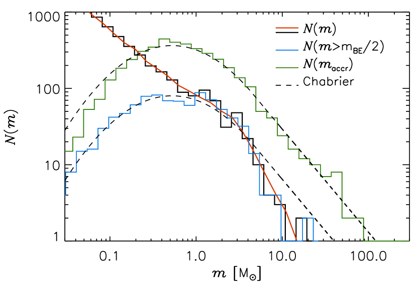
Figure 4.— Black histogram: CMF at time $t=t_{0}$. Blue histogram: CMF for a prestellar core subsample with masses $m(t_{0})>m_{\rm BE}/2$. The same CMF derived from five different realizations of the same model is shown by the red solid line. Green histogram: Model IMF at the time $t=2t_{0}$. Dashed lines: Chabrier (2005) system IMFs, shifted in mass by a factor of 2.1.

4. Conclusions

We have computed the observable CMF predicted by the PN02 IMF model, assuming characteristic MC parameters that are shown to yield a Chabrier (2005) system IMF with $\epsilon\approx 0.48$. Our main results are the following: 1) The observed mass of prestellar cores is on average a few times smaller than that of the stellar systems they generate, so $\epsilon_{\rm core}>1$. 2) The CMF rises monotonically with decreasing mass, and shows a noticeable change in slope at approximately 3-5 M_⊙, depending on mean density; 3) the selection of cores with masses $m>m_{\rm BE}/2$ yields a CMF approximately consistent with the system IMF, rescaled in mass by the same factor as the model IMF, and therefore suitable to estimate the local efficiency of star formation, $\epsilon$, and its possible dependence on cloud properties; 4) Only one in five pre-brown-dwarf core candidates is a true progenitor to a brown dwarf.

We have not discussed the protostellar CMF, nor the system IMF at time $t=t_{0}$ (when relatively massive protostars are still growing in mass). The definition of the protostellar phase faces the difficulty of accounting for the rate of mass transfer between the core and the protostar (McKee & Offner, 2010). However, we have verified that with a loose definition of protostars as all the cores that have reached their final prestellar mass, $m_{\rm max}$, but not yet their total mass, $m_{\rm accr}$ (core ages between $t_{\rm BE}+t_{\rm ff}$ and $t_{\rm accr}$), the protostellar CMF is significantly shallower than the prestellar CMF, in agreement with the observations (e.g. Hatchell & Fuller, 2008; Enoch et al., 2008), and the current system IMF has a high-mass slope a bit steeper than Salpeter’s (not observationally tested yet, to our knowledge), due to the fact that more massive cores remain longer in the protostellar phase than lower mass ones.

Upcoming starless core samples from the Herschel Gould belt survey (André et al., 2010) will allow comparisons with our model predictions. In this Letter we have only discussed the results of a very large core sample and a specific set of cloud parameters, without simulating observational uncertainties and incompleteness, and thus setting aside a detailed comparison with observed CMFs for a separate work.

References

- Adams & Fatuzzo (1996) Adams, F. C. & Fatuzzo, M. 1996, ApJ, 464, 256
- Alves et al. (2007) Alves, J., Lombardi, M., & Lada, C. J. 2007, A&A, 462, L17
- André et al. (2007) André, P., Belloche, A., Motte, F., & Peretto, N. 2007, A&A, 472, 519
- André et al. (2010) André, P., Men’shchikov, A., Bontemps, S., et al. 2010, A&A, 518, L102+
- Arzoumanian et al. (2011) Arzoumanian, D., André, P., Didelon, P., et al. 2011, A&A, 529, L6+
- Belloche et al. (2011) Belloche, A., Parise, B., Schuller, F., André, P., Bontemps, S., & Menten, K. M. 2011, ArXiv e-prints
- Bonnell et al. (2001) Bonnell, I. A., Clarke, C. J., Bate, M. R., & Pringle, J. E. 2001, MNRAS, 324, 573
- Bonnor (1956) Bonnor, W. B. 1956, MNRAS, 116, 351
- Chabrier (2005) Chabrier, G. 2005, in Astrophysics and Space Science Library, Vol. 327, The Initial Mass Function 50 Years Later, ed. E. Corbelli, F. Palla, & H. Zinnecker, 41–+
- Clark et al. (2007) Clark, P. C., Klessen, R. S., & Bonnell, I. A. 2007, MNRAS, 379, 57
- Ebert (1957) Ebert, R. 1957, ZAp, 42, 263
- Enoch et al. (2008) Enoch, M. L., Evans, II, N. J., Sargent, A. I., Glenn, J., Rosolowsky, E., & Myers, P. 2008, ApJ, 684, 1240
- Enoch et al. (2007) Enoch, M. L., Glenn, J., Evans, II, N. J., Sargent, A. I., Young, K. E., & Huard, T. L. 2007, ApJ, 666, 982
- Evans et al. (2009) Evans, II, N. J., Dunham, M. M., Jørgensen, J. K., et al. 2009, ApJS, 181, 321
- Hatchell & Fuller (2008) Hatchell, J. & Fuller, G. A. 2008, A&A, 482, 855
- Hennebelle & Chabrier (2008) Hennebelle, P. & Chabrier, G. 2008, ApJ, 684, 395
- Johnstone et al. (2001) Johnstone, D., Fich, M., Mitchell, G. F., & Moriarty-Schieven, G. 2001, ApJ, 559, 307
- Johnstone et al. (2006) Johnstone, D., Matthews, H., & Mitchell, G. F. 2006, ApJ, 639, 259
- Johnstone et al. (2000) Johnstone, D., Wilson, C. D., Moriarty-Schieven, G., Joncas, G., Smith, G., Gregersen, E., & Fich, M. 2000, ApJ, 545, 327
- Kainulainen et al. (2009) Kainulainen, J., Lada, C. J., Rathborne, J. M., & Alves, J. F. 2009, A&A, 497, 399
- Könyves et al. (2010) Könyves, V., André, P., Men’shchikov, A., et al. 2010, A&A, 518, L106+
- Krumholz & McKee (2005) Krumholz, M. R. & McKee, C. F. 2005, ApJ, 630, 250
- McKee & Offner (2010) McKee, C. F. & Offner, S. S. R. 2010, ApJ, 716, 167
- Motte et al. (1998) Motte, F., Andre, P., & Neri, R. 1998, A&A, 336, 150
- Motte et al. (2001) Motte, F., André, P., Ward-Thompson, D., & Bontemps, S. 2001, A&A, 372, L41
- Nutter & Ward-Thompson (2007) Nutter, D. & Ward-Thompson, D. 2007, MNRAS, 374, 1413
- Onishi et al. (2002) Onishi, T., Mizuno, A., Kawamura, A., Tachihara, K., & Fukui, Y. 2002, ApJ, 575, 950
- Padoan et al. (2006) Padoan, P., Juvela, M., Kritsuk, A., & Norman, M. L. 2006, ApJ, 653, L125
- Padoan et al. (2009) —. 2009, ApJ, 707, L153
- Padoan & Nordlund (2002) Padoan, P. & Nordlund, Å. 2002, ApJ, 576, 870
- Padoan & Nordlund (2011) —. 2011, ApJ, 730, 40
- Pineda et al. (2009) Pineda, J. E., Rosolowsky, E. W., & Goodman, A. A. 2009, ApJ, 699, L134
- Rathborne et al. (2009) Rathborne, J. M., Lada, C. J., Muench, A. A., Alves, J. F., Kainulainen, J., & Lombardi, M. 2009, ApJ, 699, 742
- Stanke et al. (2006) Stanke, T., Smith, M. D., Gredel, R., & Khanzadyan, T. 2006, A&A, 447, 609
- Testi & Sargent (1998) Testi, L. & Sargent, A. I. 1998, ApJL, 508, L91