Abstract

A way of construction of semiclassical wave function (SWF) based on the Maslov - Fedoriuk approach is proposed which appears to be appropriate also for systems with chaotic classical limits. Some classical constructions called skeletons are considered. The skeletons are generalizations of Arnolds’ tori able to gather chaotic dynamics. SWF’s are continued by caustic singularities in the configuration space rather then in the phase space using complex time method. The skeleton formulation provides us with a new algorithm for the semiclassical approximation method which is applied to construct SWF’s as well as to calculate energy spectra for the circular and rectangular billiards as well as to construct the simplest SWF’s and the respective spectrum for the Bunimovich stadium. The scar phenomena are considered and a possibility of their description by the skeleton method is discussed.

PACS number(s): 03.65.-w, 03.65.Sq, 02.30.Jr, 02.30.Lt, 02.30.Mv

Key Words: Schrödinger equation, semiclassical expansion, Lagrange manifolds, classical

trajectories, chaotic dynamics, quantum chaos, scars

1 Introduction

The semiclassical approximation is widely used and by this it is the well known method of approximation in quantum physics. There are two basic formulations of the method - the one based on the wave function formulation of quantum mechanics [1, 6] and the other - on the Feynman paths integral [2, 3]. While both the formulations of quantum mechanics are known to be equivalent the general wave function formulation of the semiclassical approximation [6] is considered to be not applicable in higher dimensional quantum problems which classical limits are chaotic.

In fact it is a common convince that the only way to formulate the method in the last cases is the Gutzwiller approach based on the Feynman paths integral [4]. This convince follows from also a common believe that the wave function formalism can be applied only in the cases when the classical limit of the quantum problem is the integrable one i.e. if the classical motion is set on the Arnold tori [5, 7] on which the semiclassical wave functions (SWF) are constructed. As the main argument for such a believe the KAM theorem [5, 7] is invoked which claims that the Arnold tori structure of the classical phase space disappears if classical systems become non-integrable. It is argued that because of that the only phase space finite structure which still survive in chaotic motion of the classical system are periodic orbits which therefore provide us with a skeleton on which the Gutzwiller formula is built.

However one can criticise the point of view that the existence of the Arnold tori structure of the phase space is necessary for a possibility to construct the semiclassical wave function, i.e. that Arnold’s tori provide us with a unique support for such a construction. Such a definite conclusion does certainly not follow from the original local approach of Maslov and Fedoriuk to construct SWF’s [6].

On the other hand while the results provided by the Gutzwiller method are very rich and appreciated, particularly when energy spectra of the chaotic systems are considered (see for example [8]), the method itself does not allow us for constructing and discussing properties of the wave functions involved in the problems considered. In fact the wave functions are found in such cases by different methods mostly numerically. It is just due to such numerical calculations of the wave functions [9, 10] that a phenomenon of scars has been discovered [14] which existence in the wave function patterns is still waiting for its full explanation [16, 19, 15] (see also other papers cited in [16]).

Billiards while a non-analytic motion area are well known however as examples of the non-integrable two dimensional systems except the known cases of the elliptical and rectangular billiards. They are widely considered as a simple field of experimental [17, 18] as well as theoretical [20, 21, 22, 23] (and papers cited there) and computational investigations [9, 11, 12, 13] allowing to apply many different methods (see Sarnak’s lecture [24] and [25] of the same author for an extensive review of the respective theoretical methods covering also billiards manifolds).

In this paper we are going to develop the SWF formalism which can be applied at least in principle to non-integrable cases of the two dimensional motions in billiards and which can be easily extended to higher dimensions.

Essentially our approach is initially very close to the one of Maslov and Fedoriuk [6]. The main difference between them is in a treatment of crossing the singular points of the SWF’s set on caustics. Namely, instead of making the canonical phase space variable transformations accompanied by the Fourier transformations of the SWF’s to move through the caustic points we apply the analytical continuation on the complex time plane to both the SWF’s and the classical trajectories. This greatly simplifies the corresponding procedure in comparison with the Maslov and Fedoriuk treatment. It is the exceptional role played by the time variable in the semiclassical limit of the Schrödinger equation which permits us for such simplification. Because of this the SWF can be considered as depending effectively on the time variable only while the remaining variables plays the role of spectators.

Therefore the SWF’s are first constructed locally on so called bundles of rays to satisfy vanishing boundary conditions. Next they are matching to get a global semiclassical solution. This is done however with the help of an earlier constructed set of reversible in time closed connected ray bundles called bundle skeleton which play a role of Arnold’s tori except that a number of ray bundles in the skeleton can be infinite.

This is just the notion of the ray bundles which allows us to catch a possible chaotic motion in the billiards not to resign from considerations of a set of trajectories on which SWF’s can be defined while the bundle skeleton idea allows us to close the matching procedure of SWF’s constructed locally.

The paper is organized as follows.

In the next section the Maslov - Fedoriuk method of the semiclassical wave function construction is reminded and discussed.

In sec.3 the semiclassical wave function is considered as the classical objects which time evolution is described by the classical equations of motion.

In sec.4 the construction of global SWF’s in billiards is given.

In sec.5 the circular billiards is considered to demonstrate how the method works in the case of the presence of caustic.

In sec.6 the rectangular billiards is considered as the case deprived of a caustic.

In sec.7 our method is applied to the Bunimovich stadium to show its usefulness in describing the so called bounces ball modes.

In sec.8 we discuss a possibility to describe by the skeleton idea the scar phenomenon considering such a scar formed around the horizontal periodic orbit in the Bunimovich stadium.

In sec.9 the results of the paper are summarized and some limitations of the method are discussed.

There are four appendixes attached to the paper which justify the main assumptions used in the construction of the global SWF’s on skeletons.

2 Semiclassical wave function expansion for $n$-D stationary Schrödinger equation

Consider the $n$-dimensional stationary Schrödinger equation:

$$\bigtriangleup\Psi({\bf r})+\lambda^{2}\frac{2m}{\hbar^{2}}(E-V({\bf r}))\Psi({\bf r})=0$$ (1)

with a potential $V({\bf r}),\;{\bf r}\in R_{n}$ confining a point particle with a mass $m$ and containing a formal dimensionless parameter $\lambda>0$. For a convenience we shall put further $\hbar=1$ and $m=1$. The Schrödinger equation is recovered by putting $\lambda=1$ in (1).

We would like to construct a solution to Eq.(1) using the idea of Maslov et al [6] and considering the wave function $\Psi({\bf r})$ as defined on families of classical trajectories a dynamic of which is given by the classical Hamiltonian $H=\frac{1}{2}{\bf p}^{2}+V({\bf r})$ and which carry an energy $E_{0}$ all.

Such families are constructed locally in the following way. In $R_{n}$ we choose a $n-1$-D hypersurface $\Sigma_{n-1}$ on which the initial momenta ${\bf p}({\bf r}_{0}),\;{\bf r}_{0}\in\Sigma_{n-1}$, will be defined so that the pair $({\bf r}_{0},{\bf p}({\bf r}_{0})),\;{\bf r}_{0}\in\Sigma_{n-1}$ will serve as initial data for the trajectory ${\bf r}(t)={\bf f}({\bf r}_{0},{\bf p}({\bf r}_{0});t)$. Then the transformation: ${\bf r}\to(t,{\bf r}_{0})\to(t,s_{1},...,s_{n-1}),\;{\bf r}\equiv(x_{1},...,x_{n}),\;{\bf r}_{0}\equiv(x_{0,1}(s_{1},...,s_{n-1}),...,\linebreak x_{0,n}(s_{1},...,s_{n-1}))$, (($s_{1},...,s_{n-1}$) parameterize the hypersurface $\Sigma_{n-1}$) is one-to-one up to a caustic surface $C_{n-1}$ on which the Jacobean (${\bf f}({\bf r}_{0},{\bf p}({\bf r}_{0});t)\equiv{\bar{\bf f}}(t,s_{1},...,s_{n-1})$):

$$J(t,s_{1},...,s_{n-1})=\left|\frac{\partial{\bar{f}}_{i}}{\partial t},\frac{\partial{\bar{f}}_{i}}{\partial s_{j}}\right|$$ (2)

vanishes.

A $n$-dimensional domain $\Lambda_{n}$ of $2n$-dimensional phase space $R_{2n}$ made in this way by the hypersurface $\Sigma_{n-1}$ and trajectories emerging from it is known as the Lagrange manifold [5].

Therefore in the variables $t,s_{1},...,s_{n-1}$ the new wave function $\chi(t,s_{1},...,s_{n-1})$ satisfies the following relation with the previous one:

$$|\chi(t,s_{1},...,s_{n-1})|^{2}=|\Psi({\bar{\bf f}}(t,s_{1},...,s_{n-1})|^{2}|J(t,s_{1},...,s_{n-1})|$$ (3)

The particle momentum ${\bf p}$ on the trajectories ${\bf r}(t)={\bar{\bf f}}(t,s_{1},...,s_{n-1})$ satisfies of course the equation:

$$\frac{\partial{\bar{\bf f}}(t,s_{1},...,s_{n-1})}{\partial t}={\bf p}({\bar{\bf f}}(t,s_{1},...,s_{n-1}))$$ (4)

defining also the Jacobean evolution. Namely:

$$\frac{\partial}{\partial t}\frac{\partial{\bar{f}}_{i}(t,s_{1},...,s_{n-1})}{\partial t}=\sum_{j=1}^{n}\frac{\partial p_{i}}{\partial x_{j}}\frac{\partial{\bar{f}}_{j}(t,s_{1},...,s_{n-1})}{\partial t}$$

$$\frac{\partial}{\partial t}\frac{\partial{\bar{f}}_{i}(t,s_{1},...,s_{n-1})}{\partial s_{l}}=\sum_{j=1}^{n}\frac{\partial p_{i}}{\partial x_{j}}\frac{\partial{\bar{f}}_{j}(t,s_{1},...,s_{n-1})}{\partial s_{l}}$$

$$l=1,...,n-1$$ (5)

so that

$$\frac{\partial J(t,s_{1},...,s_{n-1})}{\partial t}=J(t,s_{1},...,s_{n-1})\nabla{\bf p}({\bar{\bf f}}(t,s_{1},...,s_{n-1}))$$ (6)

The above equation is just the Liouville theorem with the solution:

$$J(t,s_{1},...,s_{n-1})=J(s_{1},...,s_{n-1})e^{\int_{0}^{t}\nabla{\bf p}({\bar{\bf f}}(t^{\prime},s_{1},...,s_{n-1}))dt^{\prime}}$$ (7)

where $J(s_{1},...,s_{n-1})$ is the value of the Jacobean on the hypersurface $\Sigma_{n-1}$.

It is well known from the classical Hamiltonian mechanics [5] that the action integral:

$$S({\bf r},{\bf r}_{0})=\int_{{\bf r}_{0}}^{\bf r}{\bf p}({\bf r}^{\prime})d{\bf r}^{\prime}$$ (8)

taken on the Lagrange manifold $\Lambda_{n}$ is a point function of ${\bf r}$ and ${\bf r}_{0}$. Therefore taking ${\bf r}_{0}$ as a definite fixed point of the hypersurface $\Sigma_{n-1}$ and denoting by $S({\bf r})$ the action function corresponding to this case we can complete a definition of the wave function $\chi(t,s_{1},...,s_{n-1})$ by the following equation:

$$\Psi^{\sigma}({\bar{\bf f}}(t,s_{1},...,s_{n-1}))=J^{-\frac{1}{2}}(t,s_{1},...,s_{n-1}))e^{\sigma\lambda iS({\bar{\bf f}}(t,s_{1},...,s_{n-1})}\chi^{\sigma}(t,s_{1},...,s_{n-1})$$

(9)

where $\sigma=\pm$ is a signature of $\Psi^{\sigma}({\bf r})$.

Therefore the quantities involved in the above definitions satisfy the following equations:

$${\bf p}({\bf r})=\nabla S({\bf r})$$

$$\frac{1}{2}{\bf p}^{2}({\bf r})+V({\bf r})-E_{0}=0$$

$$\triangle(J^{-\frac{1}{2}}\chi^{\sigma}({\bf r}))+\sigma 2i\lambda J^{-\frac{1}{2}}({\bf r})\nabla\chi^{\sigma}({\bf r})\cdot{\bf p}({\bf r})+2\lambda^{2}(E-E_{0})J^{-\frac{1}{2}}({\bf r})\chi^{\sigma}({\bf r})=0$$

$${\bf r}={\bar{\bf f}}(t,s_{1},...,s_{n-1})$$ (10)

By the variables $t,s_{1},...,s_{n-1}$ the third of the last equations can be rewritten in the following form:

$$\sigma 2i\lambda\frac{\partial\chi^{\sigma}(t,s_{1},...,s_{n-1},\lambda)}{\partial t}+$$

$$J^{\frac{1}{2}}\triangle\left(J^{-\frac{1}{2}}\chi^{\sigma}(t,s_{1},...,s_{n-1},\lambda)\right)+\lambda^{2}(E-E_{0})\chi^{\sigma}(t,s_{1},...,s_{n-1},\lambda)=0$$ (11)

where a dependence of $\chi^{\sigma}(t,s_{1},...,s_{n-1},\lambda)$ on $\lambda$ was shown explicitly.

The Eq.(11) describes the time evolution of $\chi^{\sigma}(t,s_{1},...,s_{n-1},\lambda)$ along trajectories starting on the hypersurface $\Sigma_{n-1}$ if its ”initial” values on this surface, i.e. $\chi^{\sigma}(0,s_{1},...,s_{n-1},\lambda)\equiv\chi^{\sigma}(s_{1},...,s_{n-1},\lambda)$ are given.

We are going to consider the equation (11) in the semiclassical limit $\lambda\to+\infty$ looking for its solutions in the form of the following asymptotic series:

$$E-E_{0}=\sum_{k\geq 1}E_{k}\lambda^{-k-1}$$

$$\chi^{\sigma}(t,s_{1},...,s_{n-1},\lambda)=\sum_{k\geq 0}\chi_{k}^{\sigma}(t,s_{1},...,s_{n-1})\lambda^{-k}$$

$$\chi^{\sigma}(s_{1},...,s_{n-1},\lambda)=\sum_{k\geq 0}\chi_{k}^{\sigma}(s_{1},...,s_{n-1})\lambda^{-k}$$ (12)

Putting $\lambda=1$ in (1), (9) and (12) we get approximate semiclassical solutions to the energy eigenvalue problem of the Schrödinger equation.

It is to be noticed that for the selfconsistency reasons the semiclassical series for the energy parameter in (12) starts from the second power of $\lambda^{-1}$, i.e. this ensures the proper hierarchy of steps in the algorithm of semiclassical calculations by which the higher order terms of the series in (12) are determined by the lower order ones.

It should be noticed also that despite the fact that $E_{0}$ enters the classical equation of motion (10) it is still quantum, i.e. its value depends on $\hbar$ which is considered to have the definite numerical value, i.e. $\hbar$ is not a parameter. In particular the series (12) represent the inverse power hierarchy in the formal parameter $\lambda$, i.e. not in powers of $\hbar$, between subsequent terms.

Moreover $E_{0}$ if quantized can depend on $\lambda$. However, whatever is this dependence the semiclassical series of the difference $E-E_{0}$ must be given by (12).

Needless to say the introducing $\lambda$ makes a treatment of the Schrödinger equation equivalent of course to considering it in the limit $\hbar\to 0$, i.e. semiclassically, clearly however separating the role of $\hbar$ as a parameter from its role defining the microscale of quantum phenomena.

Substituting (12) into (11) we get:

$$\frac{\partial\chi_{0}^{\sigma}(t,s_{1},...,s_{n-1})}{\partial t}=0$$

$$\frac{\partial\chi_{k+1}^{\sigma}(t,s_{1},...,s_{n-1})}{\partial t}=$$

$$\frac{\sigma i}{2}\left(J^{\frac{1}{2}}\triangle\left(J^{-\frac{1}{2}}\chi_{k}^{\sigma}(t,s_{1},...,s_{n-1})\right)+2\sum_{l=0}^{k}E_{k-l+1}\chi_{l}^{\sigma}(t,s_{1},...,s_{n-1})\right)$$

$$k=0,1,2,...,$$ (13)

with the obvious solutions:

$$\chi_{0}^{\sigma}(t,s_{1},...,s_{n-1})\equiv\chi_{0}^{\sigma}(s_{1},...,s_{n-1})$$

$$\chi_{k+1}^{\sigma}(t,s_{1},...,s_{n-1})=\chi_{k+1}^{\sigma}(s_{1},...,s_{n-1})+$$

$$\frac{\sigma i}{2}\int_{0}^{t}\left(J^{\frac{1}{2}}\triangle\left(J^{-\frac{1}{2}}\chi_{k}^{\sigma}(t^{\prime},s_{1},...,s_{n-1})\right)+2\sum_{l=0}^{k}E_{k-l+1}\chi_{l}^{\sigma}(t^{\prime},s_{1},...,s_{n-1})\right)dt^{\prime}$$

$$k=0,1,2,...,$$ (14)

3 Semiclassical wave function expansion elements as classical objects

The recurrent system of equations (13) can be considered also from the classical point of view as defining the time evolutions of $\chi_{k}^{\sigma}(t,s_{1},...,s_{n-1}),\;k=0,1,2,...,$ along the classical trajectories ${\bf r}(t)={\bar{\bf f}}(t,s_{1},...,s_{n-1})$. Namely, for each given initial point ${\bf r}_{0}(s_{1},...,s_{n-1})$ and a given trajectory emerging from it let $d$ denotes a distance measured along the trajectory from the point ${\bf r}_{0}(s_{1},...,s_{n-1})$ to the point $(x_{1},...,x_{n})$ lying on this trajectory. The set $(d,s_{1},...,s_{n-1})$ can be used as the new coordinates instead of $(x_{1},...,x_{n})$. Their mutual relations are given by:

$$d={\bar{d}}(t,s_{1},...,s_{n-1})=\int_{0}^{t}\left|\frac{\partial{\bar{\bf f}}(t^{\prime},s_{1},...,s_{n-1})}{\partial t^{\prime}}\right|dt^{\prime}$$ (15)

and

$${\bf r}=(x_{1},...,x_{n})={\bar{\bf f}}({\bar{t}}(d,s_{1},...,s_{n-1}),s_{1},...,s_{n-1})\equiv{\bf g}(d,s_{1},...,s_{n-1})$$ (16)

where $t={\bar{t}}(d,s_{1},...,s_{n-1})$ is the solution of $d={\bar{d}}(t,s_{1},...,s_{n-1})$ with respect to $t$.

Considered on the Lagrange manifold $\Lambda_{n}$ the system is then governed by the Hamiltonian:

$${\bar{H}}_{\Lambda_{n}}=\frac{1}{2}\frac{p_{d}^{2}}{\left|\frac{\partial{\bf g}(d,s_{1},...,s_{n-1})}{\partial d}\right|^{2}}+{\bar{V}}(d,s_{1},...,s_{n-1})$$ (17)

where ${\bar{V}}(d,s_{1},...,s_{n-1})\equiv V({\bar{\bf f}}({\bar{t}}(d,s_{1},...,s_{n-1}),s_{1},...,s_{n-1}))$ and $p_{d}$ is the momentum conjugated with $d$.

The corresponding classical equation of motion for ${\chi}^{\sigma}(t,s_{1},...,s_{n-1},\lambda)$ on the manifold $\Lambda_{n}$ is therefore:

$$\frac{d\chi^{\sigma}(t,s_{1},...,s_{n-1},\lambda)}{dt}=\{\chi^{\sigma},{\bar{H}}_{\Lambda_{n}}\}+\frac{\partial\chi^{\sigma}(t,s_{1},...,s_{n-1},\lambda)}{\partial t}=\frac{\partial\chi^{\sigma}(t,s_{1},...,s_{n-1},\lambda)}{\partial t}$$ (18)

since $\chi^{\sigma}(t,s_{1},...,s_{n-1},\lambda)$ being independent of $d$ commutes with the hamiltonian ${\bar{H}}_{\Lambda_{n}}$.

Therefore, from (12) and (13) we get on the Lagrange manifold $\Lambda_{n}$:

$$\frac{d{\chi}_{0}^{\sigma}(t,s_{1},...,s_{n-1})}{dt}=0$$

$$\frac{d{\chi}_{k+1}^{\sigma}(t,s_{1},...,s_{n-1})}{dt}=\frac{\sigma i}{2}J^{\frac{1}{2}}\triangle\left(J^{-\frac{1}{2}}{\chi}_{k}^{\sigma}(t,s_{1},...,s_{n-1})\right)+\sigma i\sum_{l=0}^{k}E_{k-l+1}{\chi}_{l}^{\sigma}(t,s_{1},...,s_{n-1})$$

$$k=0,1,2,...,\;\;\;\;\;\;\;\;\;$$ (19)

Of course (14) provides the solution to the equations (19).

To conclude $\chi_{0}^{\sigma}(t,s_{1},...,s_{n-1})$ is constant on the Lagrange manifold $\Lambda_{n}$ according to (14) being obviously independent also of $d$.

It is to be noticed that defining on $\Sigma_{n-1}$ another Lagrange manifold $\Lambda_{n}^{\prime}$ by choosing a different set of trajectories we obtain also another SWF defined on this new Lagrange manifold, i.e. different from the one defined on $\Lambda_{n}$. This is why the corresponding $\chi_{0}^{\sigma}(t,s_{1},...,s_{n-1})$ cannot be considered as the global integral of motion, i.e. in the whole phace space $R_{2n}$ of the Hamiltonian $H$ - each particular SWF is defined only on a particular Lagrange manifold $\Lambda_{n}$ corresponding to it.

For future applications it is worth to note that if (11) is obviously invariant on a reparametrization of the hypersurface $\Sigma_{n-1}$ it is also invariant on the following change of variables:

$$t\to\tau(s_{1},...,s_{n-1})-t$$

$$s_{k}\to h_{k}(s_{1},...,s_{n-1})$$

$$k=1,...,n-1$$ (20)

if it is accompanied simultaneously by the transformations:

$$\chi^{\sigma}(t,s_{1},...,s_{n-1},\lambda)\to$$

$${\chi}^{-\sigma}(t,s_{1},...,s_{n-1},\lambda)\equiv J_{1}^{-\frac{1}{2}}(h_{1}^{-1}(s_{1},...,s_{n-1}),...,h_{n-1}^{-1}(s_{1},...,s_{n-1}))\times$$

$$\chi^{\sigma}(\tau(s_{1},...,s_{n-1})-t,h_{1}^{-1}(s_{1},...,s_{n-1}),...,h_{n-1}^{-1}(s_{1},...,s_{n-1}),\lambda)$$ (21)

where $J_{1}(s_{1},...,s_{n-1})$ is the Jacobean of the transformation (20).

4 Semiclassical wave functions in the billiards

Let us apply the above formalism to construct continuous semiclassical wave functions inside billiards $B$ (Fig.1) vanishing on its boundary. Such a construction will be done in several steps the first one consisting of some geometrical preliminaries describing a notion of a skeleton, i.e. the closed set of families of trajectories which forms a base on which SWF’s are constructed.

4.1 Ray bundles and bundle skeletons

We shall assume that the billiards is classical, i.e. its boundary $\partial B$ is a

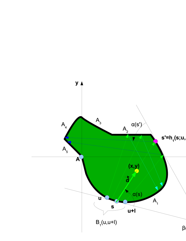
Figure 1: An arbitrary billiards

closed curve independent of $\lambda$ and given by ${\bf r}={\bf r}_{0}(s)=[x_{0}(s),y_{0}(s)]$ where $s$ is a distance of a boundary point ${\bf r}_{0}(s)$ measured clockwise along $\partial B$ from some other point $A$ of $\partial B$ chosen arbitrary, i.e. $s(A)=0$. Both $x_{0}(s)$ and $y_{0}(s)$ are continues. The curve however consists of a finite number $q,\;q\geq 1$ of smooth arcs $A_{1},...,A_{q}$ with respective length $L_{1},...,L_{q}$, so that the derivatives $x_{0}^{\prime}(s)$ and $y_{0}^{\prime}(s)$ are discontinuous in a finite number of points on the segment $0\leq s\leq L$ where $L=L_{1}+\cdots+L_{q}$ is the total length of $\partial B$. Both $x_{0}(s)$ and $y_{0}(s)$ are of course periodic with the period equal to $L$. We shall identify the point $A$ with the point beginning the arc $A_{1}$.

Next we define a bundle of rays as a family of trajectories in the following way.

Let $A_{k}(u,l),\;L_{1}+\cdots+L_{k-1}\leq u\leq L_{1}+\cdots+L_{k},\;0<l\leq L_{k},$ be an open connected piece of the arc $A_{k}$ beginning at $s=u$ and having a length $l$.

Let further ${\bf r}_{k}(s,t;u,l),\;u<s<u+l,\;0\leq t,$ be a family of trajectories given by angles $\gamma_{k}(s;u,l),\;0\leq\gamma_{k}(s;u,l)\leq 2\pi$, at which the trajectories escape from $A_{k}(u,l)$. The angles $\gamma(s;u,l)$ are smooth functions of $s$ and are measured with respect to the $x$-axis while the tangential vectors ${\bf t}(s)=[\frac{dx_{0}(s)}{ds},\frac{dy_{0}(s)}{ds}]=[\cos\beta(s),\sin\beta(s)]$ are inclined to the $x$-axis at angles $\beta(s)$ (Fig.1). The latter angle can be discontinuous at the points where $x_{0}^{\prime}(s)$ and $y_{0}^{\prime}(s)$ are discontinuous. Then the angle $\alpha_{k}(s;u,l)=\gamma_{k}(s;u,l)-\beta_{k}(s)$ is made by the classical ball momentum ${\bf p}(s;u,l)$ on the trajectory with the tangent vector ${\bf t}(s)$, i.e. ${\bf p}(s;u,l)\cdot{\bf t}(s)=p\cos\alpha_{k}(s;u,l)$. It is assumed that $0<\alpha_{k}(s;u,l)<\pi$.

The classical time evolution of the family ${\bf r}_{k}(s,t;u,l),\;u<s<u+l,$ is therefore the following

$${\bf r}_{k}(s,t;u,l)={\bf r}_{0}(s)+{\bf p}(s;u,l)t,\;\;\;\;\;\;{\bf r}_{0}(s)\in A_{k}$$ (22)

where ${\bf p}(s;u,l)=[p\cos\gamma_{k}(s;u,l),p\sin\gamma_{k}(s;u,l)]$ satisfies the classical equations of motions (10), i.e. ${\bf p}^{2}(s;u,l)=2E_{0}$ (again we put $m=1$ for the billiard ball mass).

The trajectories (22) define of course the change of variables $(x,y)\to(t,s)$, in vicinity of $A_{k}(u,l)$, i.e. $x=f_{k}(t,s;u,l),\;y=g_{k}(t,s;u,l)$ with the Jacobean:

$${\tilde{J}}_{k}(t,s;u,l)=p^{2}\gamma_{k}^{\prime}(s;u,l)t-p\left|{\bf t}(s)\right|\sin\alpha_{k}(s;u,l)=p^{2}\gamma_{k}^{\prime}(s;u,l)t-p\sin\alpha_{k}(s;u,l)$$

(23)

since $\left|{\bf t}(s)\right|=1$.

The family of trajectories defined in the above way will be called a bundle of rays emerging from the segment $A_{k}(u,l)$ of $A_{k}$ and will be denoted by $B_{k}(u,l)$ while the trajectory itself will be called rays.

Since each ray of the bundle $B_{k}(u,l)$ after some time $\tau_{k}(s;u,l),\;{\bf r}_{0}(s)\in A_{k}(u,l)$, (different for different rays) achieves another point of the boundary $\partial B$ it means that the bundle $B_{k}(u,l)$ maps the segment $A_{k}(u,l)$ into another piece $BA_{k}(u,l)$ of the boundary $\partial B$. In general it is assumed that this map of $A_{k}(u,l)$ into $BA_{k}(u,l)$ provided by the transformation (22) is one-to-one except the caustic points of $BA_{k}(u,l)$ in which ${\tilde{J}}_{K}(\tau_{k}(s;u,l),h_{k}(s;u,l);u,l)=0,\;{\bf r}_{0}(h_{k}(s;u,l))\in BA_{k}(u,l)$. Here $h_{k}(s;u,l),\;{\bf r}_{0}(s)\in A_{k}(u,l)$, realizes explicitly this map. The caustic points will be assumed to be isolated singular points of the map $A_{k}(u,l)\to BA_{k}(u,l)$. Typically they need a special care if they are.

By $DB_{k}(u,l)$ will be denoted a domain of the billiards $B$ covered by rays of the bundle $B_{k}(u,l)$ emerging from $A_{k}(u,l)$ and ending at $BA_{k}(u,l)$. The domain $DB_{k}(u,l)$ is locally a Lagrangian manifold on which each loop integral $\oint{\bf p}\cdot d{\bf r}$ vanishes.

Assume further the boundary $\partial B$ to be a mirror-like, i.e. reflecting the incoming rays according to the reflection principle of the geometrical optics and let $A_{k^{\prime}}(u^{\prime},l^{\prime})$ be a piece of another arc $A_{k^{\prime}}$ of $\partial B$ such that $A_{k^{\prime}}(u^{\prime},l^{\prime})\cap BA_{k}(u,l)\neq\oslash$ on which another bundle of rays $B_{k^{\prime}}(u^{\prime},l^{\prime})=\{{\bf r}_{k^{\prime}}(s,t;u^{\prime},l^{\prime}):u^{\prime}<s<u^{\prime}+l^{\prime},\;0\leq t\}$ is defined.

If on the segment $A_{k^{\prime}}(u^{\prime},l^{\prime})\cap BA_{k}(u,l)$ the ray bundle $B_{k^{\prime}}(u^{\prime},l^{\prime})$ coincides with the reflected one we call the ray bundle $B_{k^{\prime}}(u^{\prime},l^{\prime})$ a reflection of the bundle $B_{k}(u,l)$ on the segment mentioned.

The reflection operation over the bundle $B_{k}(u,l)$ will be denoted by $\Pi$ so that $\Pi B_{k}(u,l)$ denotes the set of all rays arising by the reflection of the bundle $B_{k}(u,l)$ of $\partial B$.

Consider now a family of the disjoint ray bundles ${\bf B}=\bigcup B_{k}(u,l),\;B_{k}(u,l)\cap B_{k^{\prime}}(u^{\prime},l^{\prime})=\oslash$ if $B_{k}(u,l)\neq B_{k^{\prime}}(u^{\prime},l^{\prime})$.

The family B will be called closed under reflection $\Pi$ on the boundary $\partial B$ if the following two conditions are satisfied for each bundle $B_{k}(u,l)\in{\bf B}$:

$$\Pi B_{k}(u,l)=\bigcup_{j=1}^{n}B_{j}(u_{j},l_{j})\cap\Pi B_{k}(u,l),\;\;\;\;\;\;\;B_{j}(u_{j},l_{j})\in A_{i_{j}},\;j=1,...,n$$

$$B_{k}(u,l)=\bigcup_{i=1}^{m}\Pi B_{i}(u_{i},l_{i})\cap B_{k}(u,l),\;\;\;\;\;\;\;B_{i}(u_{i},l_{i})\in A_{j_{i}},\;i=1,...,m$$

$$\Pi{\bf B}={\bf B}$$ (24)

A closed family ${\bf B}^{\prime}=\bigcup B_{k^{\prime}}(u^{\prime},l^{\prime})$ is embedded into a closed family ${\bf B}=\bigcup B_{k}(u,l)$ if each ray bundle of ${\bf B}^{\prime}$ is a subset of some ray bundle of ${\bf B}$ and each bundle of ${\bf B}$ contains some bundle of ${\bf B}^{\prime}$.

A closed bundle family is called connected if it cannot be decomposed into a sum of another two disjoint closed bundle families.

A closed connected bundle family will be called a Lagrange bundle skeleton or simply a skeleton if it cannot be embedded into another closed connected bundle family.

From now on all considered bundle families will be assumed to be skeletons.

A basic property of each ray belonging to a skeleton ${\bf B}$ is that by its time evolution and bounces on the billiards boundary it will never leave ${\bf B}$.

Another basic property of a skeleton ${\bf B}$ is its completeness, i.e. none bundle can be added to or removed from the skeleton not destroying it.

Let us now reverse in time all trajectories belonging to ${\bf B}$. This operation leads us again to some skeleton ${\bf B}^{A}$ which will be called associated with ${\bf B}$.

Bundles of ${\bf B}^{A}$ are obtained simply from the corresponding bundles of ${\bf B}$. Namely with each bundle $B_{k}(u,l)$ of ${\bf B}$ let us associate a bundle $B_{k}^{A}(u,l)$ which trajectories satisfy the following condition:

$$\gamma_{k}^{A}(s;u,l)=\pi+2\beta(s)-\gamma_{k}(s;u,l),\;\;\;\;u<s<u+l$$ (25)

i.e. these trajectories are just the reflections on $\partial B$ of the time reversed trajectories defined by $\gamma_{k}(s;u,l)$ and belonging to $B_{k}(u,l)$.

The skeleton ${\bf B}^{A}$ is organized by all bundles $B_{k}^{A}(u,l)$ obtained in the above way.

4.2 SWF’s defined on ray bundles of a bundle skeleton

Consider a bundle skeleton ${\bf B}$. On each of its ray bundle $B_{k}(u,l)$ we can now define the following pair of SWF’s $\Psi_{k}^{\sigma}(t,s;u,l;\lambda),\;\sigma=\pm$:

$$\Psi_{k}^{\sigma}(t,s;u,l;\lambda)={\tilde{J}}_{k}^{-\frac{1}{2}}(t,s;u,l)e^{\sigma i\lambda\left(p^{2}t+p\int_{0}^{s}\cos\alpha_{k}(s;u,l)ds^{\prime}\right)}\chi_{k}^{\sigma}(t,s;u,l;\lambda)$$ (26)

where $p^{2}=2E_{0}$ and $\chi_{k}^{\sigma}(t,s;u,l;\lambda),\;\sigma=\pm$, are given by (12) and (14).

Exactly in the same way we can define a pair $\Psi_{A;k}^{\sigma}(t,s;u,l;\lambda),\;\sigma=\pm$, of SWF’s on the corresponding associated bundle $B_{k}^{A}(u,l)$:

$$\Psi_{A;k}^{\sigma}(t,s;u,l;\lambda)={\tilde{J}}_{A;k}^{-\frac{1}{2}}(t,s;u,l)e^{\sigma i\lambda\left(p^{2}t-p\int_{0}^{s}\cos\alpha_{k}(s;u,l)ds^{\prime}\right)}\chi_{A;k}^{\sigma}(t,s;u,l;\lambda)$$ (27)

It will be also convenient for further considerations to substitute the time variable $t$ by the distance variable $d=pt$ and consequently to give the trajectories (22), the Jacobean (23) and the wave function (26) the following forms:

$${\bf r}_{k}(d,s;u,l)={\bf r}_{0}(s)+{\bf d}(s;u,l)$$

$${\bf d}(s;u,l)={\bf p}t=[d\cos\gamma_{k}(s;u,l),d\sin\gamma_{k}(s;u,l)]$$

$${\bf r}_{0}(s)\in A_{k}(u,l)$$ (28)

and

$$J_{k}(d,s;u,l)=\frac{1}{p}{\tilde{J}}_{k}(t,s;u,l)=\frac{\partial\gamma_{k}(s;u,l)}{\partial s}d-\sin\alpha_{k}(s;u,l)$$

$${\bf r}_{0}(s)\in A_{k}(u,l)$$ (29)

and

$$\Psi_{k}^{\sigma}(d,s;u,l;\lambda)=J_{k}^{-\frac{1}{2}}(d,s;u,l)e^{\sigma ik\left(d+\int_{0}^{s}\cos\alpha_{k}(s^{\prime};u,l)ds^{\prime}\right)}{\bar{\chi}}_{k}^{\sigma}(d,s;u,l;\lambda)$$

$${\bf r}_{0}(s)\in A_{k}(u,l)$$ (30)

where ${\bar{\chi}}_{k}^{\sigma}(d,s;u,l;\lambda)\equiv p\chi_{k}^{\sigma}(\frac{d}{p},s;u,l;\lambda),\;\sigma=\pm$, and $k=p\lambda$ is the wave number of the billiards ball.

Nevertheless, for simplicity of notations, the bar over ${\bar{\chi}}_{k}^{\sigma}(d,s;u,l;\lambda)$ will be dropped in our further considerations.

By the variable $d$ the solutions (14) can be rewritten in the form:

$${\chi}_{k,0}^{\sigma}(d,s;u,l)\equiv{\chi}_{k,0}^{\sigma}(s;u,l)$$

$${\chi}_{k,j+1}^{\sigma}(d,s;u,l)={\chi}_{k,j+1}^{\sigma}(s;u,l)+$$

$$\frac{\sigma i}{2p}\int_{0}^{d}\left(D_{k}(a,s;u,l){\chi}_{k,j}^{\sigma}(a,s;u,l)+2\sum_{m=0}^{j}E_{j-m+1}{\chi}_{k,m}^{\sigma}(a,s;u,l)\right)da$$

$$j=0,1,2,...,$$ (31)

where $D_{k}(d,s;u,l)=J_{k}^{\frac{1}{2}}(d,s;u,l)\cdot\triangle_{k}(d,s;u,l)\cdot J_{k}^{-\frac{1}{2}}(d,s;u,l)$ and $\triangle_{k}(d,s;u,l)$ is the Laplacean expressed by the variables $d$ and $s$ corresponding to the $B_{k}(u,l)$-bundle.

$\Psi_{k}^{\sigma}(d,s;u,l;\lambda),\;\sigma=\pm,$ are defined initially in the domain $D_{k}(u,l)$ of the billiards which boundary $\partial D_{k}(u,l)$ contains of course $A_{k}(u,l)$. A pattern of the remaining part of $\partial D_{k}(u,l)$ depends on the corresponding caustic $K_{k}(u,l)=\{(f_{k}(K_{k}(s;u,l),s;u,l),g_{k}(K_{k}(s;u,l),s;u,l)):$$J_{k}(K_{k}(s;u,l),s;u,l)=0,\;{\bf r}_{0}(s)\in A_{k}(u,l)\}$. It follows from (23) that

$$K_{k}(s;u,l)=\frac{\sin\alpha_{k}(s;u,l)}{\frac{\partial\gamma_{k}(s;u,l)}{\partial s}},\;\;\;\;\;\;\;{\bf r}_{0}(s)\in A_{k}(u,l)$$ (32)

and $K_{k}(s;u,l)$ can escape to infinity if $\frac{\partial\gamma_{k}(s;u,l)}{\partial s}\to 0$.

If the set $K_{k}(u,l)\cap B$ is not empty then it belongs to $\partial D_{k}(u,l)$. The remaining rays of $B_{k}(u,l)$ which are not tangent to $K_{k}(u,l)\cap B$ end at $BA_{k}(u,l)$ and complete in this way the domain $D_{k}(u,l)$.

An important property of the representation (26) is its uniqueness, i.e. for two different bundles defined on the segment $A_{k}(u,l)$ this representation provides us with two different pairs of $\Psi_{k}^{\sigma}(d,s;u,l;\lambda),\;\sigma=\pm$. This conclusion follows from the fact that for $\lambda$ sufficiently large the SWF’s are determined only by exponentials and the latter are different at the same points $(x,y)$ for different bundles.

4.3 Propagation of $\Psi_{k}^{\sigma}(d,s;u,l;\lambda)$ through a skeleton

$\Psi_{k}^{\sigma}(d,s;u,l;\lambda),\;\sigma=\pm,$ being defined in $D_{k}(u,l)\in B_{k}(u,l)$ can be continued on the whole skeleton by accepting two rules the solutions have to satisfy.

A need for the first rule to be formulated arises when the solutions propagate by the caustic where they are singular. These are branch points singularities on the $d$-plane of the type $(d-d_{c}(s))^{-\frac{1}{2}}$ where $J_{k}(d_{c}(s),s;u,l)=0$. These points have to be avoided somehow when continuing the solutions along the rays of $B_{k}(u,l)$. Relying on the results of App.B we accept the rule of avoiding these points clockwise by $\Psi_{k}^{+}(d,s;u,l;\lambda)$ and above them and anticlockwise by $\Psi_{k}^{-}(d,s;u,l;\lambda)$ and below them.

The second rule has to be given to describe bouncings of $\Psi_{k}^{\sigma}(d,s;u,l;\lambda),\;\sigma=\pm,$ by the billiards boundary.

Let $B_{k^{\prime}}(u^{\prime},l^{\prime})$ be a reflection of the bundle $B_{k}(u,l)$ i.e. $B_{k^{\prime}}(u^{\prime},l^{\prime})\subset\Pi B_{k}(u,l)$. Continuations of $\Psi_{k}^{\sigma}(d,s;u,l;\lambda),\;\sigma=\pm,$ onto $B_{k^{\prime}}(u^{\prime},l^{\prime})$ is given by the following formula:

$$\Psi_{k}^{\sigma,cont}(d,s;u^{\prime},l^{\prime};\lambda)=-\eta_{\sigma}J_{k^{\prime}}^{-\frac{1}{2}}(d,s;u^{\prime},l^{\prime})\times$$

$$e^{\sigma i\lambda p\left(d-\int_{u^{\prime}}^{s}\cos\alpha_{k^{\prime}}(s^{\prime};u^{\prime},l^{\prime})ds^{\prime}+\delta_{k}(u,l)\right)}\chi_{k}^{\sigma,cont}(d,s;u^{\prime},l^{\prime};\lambda)$$

$$\delta_{k}(u,l)=D(h_{k}^{-1}(s;u,l);u,l)+\int_{u^{\prime}}^{s}\cos\alpha_{k^{\prime}}(s^{\prime};u^{\prime},l^{\prime})ds^{\prime}-\int_{u}^{h_{k}^{-1}(s;u,l)}\cos\alpha_{k}(s^{\prime};u,l)ds^{\prime}$$

$$\chi_{k}^{\sigma,cont}(0,s;u^{\prime},l^{\prime};\lambda)=\left|\frac{\partial h_{k}(s^{\prime};u,l)}{\partial s^{\prime}}\right|_{s^{\prime}=h_{k}^{-1}(s;u,l)}^{-\frac{1}{2}}\chi_{k}^{\sigma}(D(h_{k}^{-1}(s;u,l);u,l),h_{k}^{-1}(s;u,l);u,l;\lambda)$$

$${\bf r}_{0}(s)={\bf r}_{0}(h_{k}^{-1}(s;u,l))+{\bf D}(h_{k}^{-1}(s;u,l);u,l)$$ (33)

The factor $\eta_{\sigma}$ in (33) depends on whether there was a caustic point on the way of continuations of $\Psi_{k}^{\sigma}(d,s;u,l;\lambda)$ in which case $\eta_{\sigma}=\sigma i$ but $\eta_{\sigma}\equiv 1$ in the opposite case.

$D(s;u,l)=|{\bf D}(s;u,l)|$ denotes the distance between the points ${\bf r}_{0}(h_{k}(s;u,l))$ and ${\bf r}_{0}(s)$ of the boundary $\partial B$.

It is to be noticed that $\delta_{k}(u,l)$ is $s$-independent (see App.C).

$\chi_{k}^{\sigma,cont}(d,s;u^{\prime},l^{\prime};\lambda)$ is defined by (31) with the initial values given by the corresponding semiclassical series of $\chi_{k}^{\sigma,cont}(0,s;u^{\prime},l^{\prime};\lambda)$ as given by (33). Due to the chain property of the formulae (31) such a definition of $\chi_{k}^{\sigma,cont}(d,s;u^{\prime},l^{\prime};\lambda)$ ensures that $\chi_{k}^{\sigma}(d,s;u,l;\lambda)$ can be considered as a continuous function of $d$ on the skeleton as $d$ changes along rays arising by subsequent reflections of the one starting from the bundle $B_{k}(u,l)$.

Another property of the definition (33) is that close to the arc $A_{k^{\prime}}$ there is a domain in which both the SWF’s $\Psi_{k}^{\sigma,cont}(d^{\prime},s^{\prime};u^{\prime},l^{\prime};\lambda)$ and $\Psi_{k}^{\sigma}(d,s;u,l;\lambda)$ are defined so that the superposition:

$$\Psi_{k}^{\sigma,sup}(x,y,\lambda)\equiv\Psi_{k}^{\sigma,cont}(d^{\prime},s^{\prime};u^{\prime},l^{\prime};\lambda)+\Psi_{k}^{\sigma}(d,s;u,l;\lambda)$$

$$x=x_{0}(s)+d\cos\alpha_{k}(s;u,l)=x_{0}(s^{\prime})+d^{\prime}\cos\alpha_{k^{\prime}}(s^{\prime};u^{\prime},l^{\prime})$$

$$y=y_{0}(s)+d\sin\alpha_{k}(s;u,l)=y_{0}(s^{\prime})+d^{\prime}\sin\alpha_{k^{\prime}}(s^{\prime};u^{\prime},l^{\prime})$$ (34)

can be done.

It follows easily from (33) that on the arc $A_{k^{\prime}}$, i.e. for $d^{\prime}=0$ this superposition vanishes.

4.4 SWF’s vanishing on the billiards boundary

Another obvious property of $\Psi_{k}^{\sigma}(d,s;u,l;\lambda),\;\sigma=\pm$, is that they cannot vanish on $A_{k}(u,l)$ unless $\chi_{k}^{\sigma}(d,s;u,l;\lambda)$ vanish there identically. Therefore a wave function $\Psi_{k}^{as;\sigma}(x,y;u,l;\lambda)$ vanishing on $A_{k}(u,l)$ should be represented in the semiclassical limit by a linear combination of at least two SWF’s of the form (26). The superposition (34) is an important example of such a combination. It is shown however in App.A on a more general level of considerations that the proper linear combinations have to be the following:

$$\Psi_{k}^{as;\sigma}(x,y;u,l;\lambda)=\Psi_{k}^{\sigma}(d_{1},s_{1};u,l;\lambda)+\Psi_{A;k}^{-\sigma}(d_{2},s_{2};u,l;\lambda)=$$

$$J_{k}^{-\frac{1}{2}}(d_{1},s_{1};u,l)e^{i\sigma k\left(d_{1}+\int_{0}^{s_{1}}\cos\alpha_{k}(s^{\prime};u,l)ds^{\prime}\right)}\chi_{k}^{\sigma}(d_{1},s_{1};u,l;\lambda)+$$

$$J_{A;k}^{-\frac{1}{2}}(d_{2},s_{2};u,l)e^{-i\sigma k\left(d_{2}-\int_{0}^{s_{2}}\cos\alpha_{k}(s^{\prime};u,l)ds^{\prime}\right)}\chi_{A;k}^{-\sigma}(d_{2},s_{2};u,l;\lambda)$$ (35)

with the following boundary conditions:

$$\chi_{k}^{\sigma}(0,s;u,l;\lambda)+\chi_{A;k}^{-\sigma}(0,s;u,l;\lambda)=0\;\;\;\;\;\;\;{\bf r}_{0}(s)\in A_{k}(u,l)$$ (36)

while the point $(x,y)$ is the cross point of the respective trajectories belonging to different bundles, i.e.

$${\bf r}\equiv[x,y]={\bf r}_{k}(d_{1},s_{1};u,l)={\bf r}_{0}(s_{1})+{\bf d}_{1}(s_{1};u,l)=$$

$${\bf r}_{A;k}(d_{2},s_{2};u,l)={\bf r}_{0}(s_{2})+{\bf d}_{2}(s_{2};u,l)$$

$${\bf r}_{k}(d,s;u,l)\in B_{k}(u,l),\;\;\;\;\;{\bf r}_{A;k}(d,s;u,l)\in B_{k}^{A}(u,l)$$ (37)

The vanishing superposition (35) if defined on the bundle $B_{k^{\prime}}(u^{\prime},l^{\prime})$ suggests that $\Psi_{A;k^{\prime}}^{-\sigma}(d,s;u^{\prime},l^{\prime};\lambda)$ should be related somehow to the SWF $\Psi_{k}^{\sigma}(d,h_{k}^{-1}(s;u,l);u,l);u,l;\lambda)$ defined on the bundle $B_{k}(u,l)$ which the previous one is a reflection. In the next section this relation is established as a condition matching both the solutions.

4.5 Matching solutions defined on two different bundles of a skeleton

Let now $\Psi_{k}^{as;\sigma}(x,y;u,l;\lambda)$’s be defined in the above way on the corresponding bundles of B and ${\bf B}^{A}$. Suppose that the corresponding SWF’s $\Psi_{k}^{\sigma}(d,s;u,l;\lambda),\;\sigma=\pm,$ and $\Psi_{k}^{A;\sigma}(d,s;u,l;\lambda),\;\sigma=\pm,$ which construct them can be continued along the respective bundles on which they are defined. Note that the domains $D_{k}(u,l)$ and $D_{k}^{A}(u,l)$ where these SWF’s are initially defined are then extended to $DB_{k}(u,l)$ and $DB_{k}^{A}(u,l)$ respectively. We are then faced with the problem of matching the continued solutions with the others defined on the same skeletons B and ${\bf B}^{A}$.

Anticipating the results of App.B such a matching should be done as follows.

Let $B_{k}(u,l)$ be a reflection of the bundles $B_{k_{1}}(u_{1},l_{1}),B_{k_{2}}(u_{2},l_{2}),\ldots,B_{k_{n}}(u_{n},l_{n})$ satisfying (24). Let $\Psi_{k_{1}}^{\sigma}(d,s;u_{1},l_{1};\lambda),\Psi_{k_{2}}^{\sigma}(d,s;u_{2},l_{2};\lambda),\ldots,\Psi_{k_{n}}^{\sigma}(d,s;u_{n},l_{n};\lambda)$ be defined and continued on the respective bundles $B_{k_{1}}(u_{1},l_{1}),\;B_{k_{2}}(u_{2},l_{2}),\;\ldots,B_{k_{n}}(u_{n},l_{n})$. Let further $\Psi_{A;k}^{-\sigma}(d,s;u,l;\lambda)$ be defined on the bundle $B_{k}^{A}(u,l)$ while $\Psi_{k}^{\sigma}(d,s;u,l;\lambda)$ on the bundle $B_{k}(u,l)$ being both related by the boundary condition (36).

Then we make the following identification:

$$\Psi_{A;k}^{-\sigma}(d,h(s;u_{j},l_{j});u,l;\lambda)=\Psi_{k_{j}}^{\sigma}(D(s;u_{j},l_{j})-d,s;u_{j},l_{j};\lambda)$$

$${\bf r}_{0}(h(s;u_{j},l_{j}))\in A_{k}(u,l)\cap BL(u_{j},l_{j})$$

$${\bf r}_{0}(s)\in L(u_{j},l_{j})$$

$${\bf r}_{0}(h(s;u_{j},l_{j}))={\bf r}_{0}(s)+{\bf D}(s;u_{j},l_{j}),\;\;\;\;\;j=1,...n$$ (38)

Rewritten in terms of the $\chi$-coefficients eq.(38) gives:

$$\chi_{A;k}^{-\sigma}(d,h(s;u_{j},l_{j});u,l;\lambda)=$$

$$\eta_{\sigma}e^{\sigma i\lambda p\delta(u_{j},l_{j})}\left|\frac{\partial h(s;u_{j},l_{j})}{\partial s}\right|^{-\frac{1}{2}}\chi_{k_{j}}^{\sigma}(D(s;u_{j},l_{j})-d,s;u_{j},l_{j};\lambda)$$

$$\delta(u_{j},l_{j})=D(s;u_{j},l_{j})+\int_{u_{j}}^{s}\cos\alpha_{k_{j}}(s^{\prime};u_{j},l_{j})ds^{\prime}-\int_{u}^{h(s;u_{j},l_{j})}\cos\alpha_{k}(s^{\prime};u,l)ds^{\prime}$$

$${\bf r}_{0}(h(s;u_{j},l_{j}))\in A_{k}(u,l)\cap BL(u_{j},l_{j})$$

$${\bf r}_{0}(s)\in L(u_{j},l_{j})$$

$${\bf r}_{0}(h(s;u_{j},l_{j}))={\bf r}_{0}(s)+{\bf D}(s;u_{j},l_{j}),\;\;\;\;\;j=1,...n$$ (39)

As previously $\delta(u_{j},l_{j})$ in the above formula is $s$-independent (see App.C). Due to that and due to the properties (20) and (21) the rhs of (39) satisfies (11) as it should.

Putting $d=0$ in (39) and taking into account (36) we get:

$$\chi_{k}^{\sigma}(0,h(s;u_{j},l_{j});u,l;\lambda)=-\chi_{A;k}^{-\sigma}(0,h(s;u_{j},l_{j});u,l;\lambda)=$$

$$-\eta_{\sigma}e^{\sigma i\lambda p\delta(u_{j},l_{j})}\left|\frac{\partial h(s;u_{j},l_{j})}{\partial s}\right|^{-\frac{1}{2}}\chi_{k_{j}}^{\sigma}(D(s;u_{j},l_{j}),s;u_{j},l_{j};\lambda)=$$

$$-\eta_{\sigma}e^{\sigma i\lambda p\delta(u_{j},l_{j})}\chi_{k_{j}}^{\sigma,cont}(0,h(s;u_{j},l_{j});u,l;\lambda)$$

$${\bf r}_{0}(h(s;u_{j},l_{j}))\in A_{k}(u,l)\cap BL(u_{j},l_{j})$$

$${\bf r}_{0}(s)\in L(u_{j},l_{j})$$

$${\bf r}_{0}(h(s;u_{j},l_{j}))={\bf r}_{0}(s)+{\bf D}(s;u_{j},l_{j}),\;\;\;\;\;j=1,...n$$ (40)

Comparing (40) with (33) it is easily seen that $\Psi_{k}^{\sigma}(d,s;u,l;\lambda)$ has to coincide with $\Psi_{k_{j}}^{\sigma,cont}(d,s;u,l;\lambda)$.

4.6 SWF’s defined on a bundle skeleton

Let ${\bf r}=(x,y)$ be a fixed point of the billiards. Let $D(x,y)$ denote a set of all $D(u,l)$, $B(u,l)\in{\bf B}$ which contain this point and $D_{A}(x,y)$ the respective set of $D^{A}(u,l),\;B^{A}(u,l)\in{\bf B}^{A}$. Let further $DB(x,y)$ denote a set of all $DB(u,l)$, $B(u,l)\in{\bf B}$ which contain the point $(x,y)$ and $DB^{A}(x,y)$ the respective set of $DB^{A}(u,l),\;B^{A}(u,l)\in{\bf B}^{A}$.

SWF’s $\Psi_{\bf B}^{as;\sigma}(x,y,\lambda)$ vanishing on the billiards boundary can now be defined on ${\bf B}$ and ${\bf B}^{A}$ as follows:

$$\Psi_{\bf B}^{as;\sigma}(x,y,\lambda)=$$

$$\sum_{D(u,l)\in D(x,y)}\Psi^{\sigma}(d(u,l),s(u,l);u,l;\lambda)+\sum_{D^{A}(u,l)\in D_{A}(x,y)}\Psi_{A}^{-\sigma}(d(u,l),s(u,l);u,l;\lambda)=$$

$$\sum_{DB(u,l)\in DB(x,y)}\Psi^{\sigma}(d(u,l),s(u,l);u,l;\lambda)=\sum_{DB^{A}(u,l)\in DB^{A}(x,y)}\Psi_{A}^{-\sigma}(d(u,l),s(u,l);u,l;\lambda)$$

$${\bf r}={\bf r}_{0}(s(u,l))+{\bf d}(u,l)$$ (41)

The SWF’s $\Psi^{\sigma}(d,s;u,l;\lambda)$ defined on bundles of ${\bf B}$ and $\Psi_{A}^{\sigma}(d,s;u,l;\lambda)$ defined on respective bundles of ${\bf B}^{A}$ are related with each other by the boundary conditions (36) and by matching conditions (38)-(40).

The solutions $\Psi_{\bf B}^{as;+}(x,y,\lambda)$ and $\Psi_{\bf B}^{as;-}(x,y,\lambda)$ coincide if and only if ${\bf B}={\bf B}^{A}$.

It is clear that the conditions (40) have to determine also the $\chi$-factors $\chi_{k}^{\sigma}(s;u,l;\lambda)$ for all the bundles $B_{k}(u,l)$ which are the ”initial” conditions for both $\chi_{k}^{\sigma}(d,s;u,l;\lambda)$ and $\chi_{A;k}^{\sigma}(d,s;u,l;\lambda)$, i.e. $\chi_{k}^{\sigma}(s;u,l;\lambda)\equiv\chi_{k}^{\sigma}(0,s;u,l;\lambda)\equiv-\chi_{A;k}^{\sigma}(0,s;u,l;\lambda)$. Nevertheless these conditions cannot be given arbitrarily. Just opposite all $\chi_{k}(s;u,l;\lambda)$ have to satisfy (40) in selfconsistent way. It is not easy to predict how this can be realized.

Certainly one has to take into account that $\chi_{k}^{\sigma}(s;u,l;\lambda)$ being given at the point ${\bf r}_{0}(s(u,l))$ of the bundle $B_{k}(u,l)$ are distributed along the boundary $\partial B$ by subsequent reflections of the initial ray ${\bf r}={\bf r}_{0}(s(u,l))+{\bf d}(u,l)$ which carries on $\chi_{k}^{\sigma}(d,s;u,l;\lambda)$ according the formulae (31), (33) and (40). However the ray come back eventually to the segment $A_{k}(u,l)$ defining $\chi_{k}^{\sigma}(s;u,l;\lambda)$ in some new point ${\bf r}_{0}(s^{\prime}(u,l))$ of this segment. Naturally a value of $\chi_{k}^{\sigma,cont}(D(u,l),s^{\prime}(u,l);u^{\prime},l^{\prime};\lambda)$ at this point has to coincide with $\chi_{k}^{\sigma}(s^{\prime}(u,l);u,l;\lambda)$ defined already at this point. This is just one of the selfconsistency conditions contained in (40) (see ”the last quantization condition” (49) below).

It seems difficult however to find a general systematic way of exploring the system (40) to get solutions satisfying it. Nevertheless one can always think at least minimally trying to guess reasonable solutions to this system. In the next sections we will try to use both the approaches for some particular cases of billiards.

The formulae (39) and (40) defines the conditions which the SWF’s $\chi_{k}^{\sigma}(d,h(s;u_{j},l_{j});u,l;\lambda)$ should satisfy when bouncing from the billiards boundary. Nevertheless this condition should be specified additionally with respect to its factors. Namely, taking their large $\lambda$-limit we get:

$$\chi_{k,0}^{\sigma}(h(s;u_{j},l_{j});u,l)=-\delta\left|\frac{\partial h(s;u_{j},l_{j})}{\partial s}\right|^{-\frac{1}{2}}e^{\sigma i\lambda p\delta(u_{j},l_{j})}\chi_{k_{j},0}^{\sigma}(s;u_{j},l_{j})$$

$$\chi_{k,r+1}^{\sigma}(h(s;u_{j},l_{j});u,l)=-\delta\left|\frac{\partial h(s;u_{j},l_{j})}{\partial s}\right|^{-\frac{1}{2}}e^{\sigma i\lambda p\delta(u_{j},l_{j})}\times$$

$$\left(\chi_{k_{j},r+1}^{\sigma}(s;u_{j},l_{j})+\frac{\sigma i}{2p}\int_{0}^{D(s;u_{j},l_{j})}\left(\frac{}{}J^{\frac{1}{2}}\triangle\left(J^{-\frac{1}{2}}\chi_{k_{j},r}^{\sigma}(a,s;u_{j},l_{j})\right)\right.\right.+$$

$$\left.\left.2\sum_{l=0}^{r}E_{r-l+1}\chi_{k_{j},l}^{\sigma}(a,s;u_{j},l_{j})\right)da\right)$$

$$r=0,1,2,...,$$ (42)

The above equations should be satisfied on each bundle $B_{k}(u,l)$ of the skeleton ${\bf B}$.

The first of the equations (42) should determine the classical quantities, namely the skeleton B and the ”classical” energy $E_{0}=\frac{1}{2}p^{2}$ and by them define the JWKB approximation of the SWF’s. Namely:

$$\Psi_{\bf B}^{JWKB;\sigma}(x,y,\lambda)=\sum_{DB(u,l)\in D(x,y)}\Psi^{JWKB;\sigma}(d(u,l),s(u,l);u,l)=$$

$$\sum_{DB(u,l)\in D(x,y)}J^{-\frac{1}{2}}(d(u,l),s(u,l))e^{i\lambda p\left(d(u,l)+\int_{u}^{s(u,l)}\cos\alpha(s^{\prime};u,l)ds^{\prime}\right)}\chi_{0}^{\sigma}(d(u,l),s(u,l);u,l)$$ (43)

The remaining equations determine quantum corrections to the ”classical” ones involved in (43).

However it is easy to note that for the selfconsistency of the equations (42) it is necessary for the exponent $e^{\sigma i\lambda p\delta(u_{j},l_{j})}$ to be independent of $\lambda$, i.e. we have to have on each bundle $B_{k}(u,l)$ of B:

$$\lambda p\delta_{k}(u,l)=\phi_{k}(u,l)$$

$$B_{k}(u,l)\subset{\bf B}$$ (44)

where $\delta_{k}(u,l)$ is given by (33) and $\phi_{k}(u,l)$ is a $\lambda$-independent constant.

The equations (44) have to define both the skeleton B and the energy $E_{0}=\frac{1}{2}p^{2}$.

Taking into account the last conclusions we get the following final set of the recurrent quantization conditions:

$$\lambda p\delta_{k}(u,l)=\phi_{k}(u,l)$$

$$\chi_{k,0}^{\sigma}(h(s;u_{j},l_{j});u,l)=-\delta e^{\sigma i\phi_{k_{j}}(u_{j},l_{j})}\left|\frac{\partial h(s;u_{j},l_{j})}{\partial s}\right|^{-\frac{1}{2}}\chi_{k_{j},0}^{\sigma}(s;u_{j},l_{j})$$

$$\chi_{k,r+1}^{\sigma}(h(s;u_{j},l_{j});u,l)=-\delta e^{\sigma i\phi_{k_{j}}(u_{j},l_{j})}\left|\frac{\partial h(s;u_{j},l_{j})}{\partial s}\right|^{-\frac{1}{2}}\left(\frac{}{}\chi_{k_{j},r+1}^{\sigma}(s;u_{j},l_{j})+\right.$$

$$\left.\frac{\sigma i}{2p}\int_{0}^{D(s;u_{j},l_{j})}\left(\frac{}{}J^{\frac{1}{2}}\triangle\left(J^{-\frac{1}{2}}\chi_{k_{j},r}^{\sigma}(a,s;u_{j},l_{j})\right)+2\sum_{l=0}^{r}E_{r-l+1}\chi_{k_{j},l}^{\sigma}(a,s;u_{j},l_{j})\right)da\right)$$

$$r=0,1,2,...,$$ (45)

together with:

$$\chi_{k,0}^{\sigma}(d,s;u,l)\equiv\chi_{k,0}^{\sigma}(s;u,l)$$

$$\chi_{k,r+1}^{\sigma}(d,s;u,l)=\chi_{k,r+1}^{\sigma}(s;u,l)+$$

$$\frac{\sigma i}{2p}\int_{0}^{d}\left(J^{\frac{1}{2}}\triangle\left(J^{-\frac{1}{2}}\chi_{k,r}^{\sigma}(a,s;u,l)\right)+2\sum_{m=0}^{r}E_{r-l+1}\chi_{k,m}^{\sigma}(a,s;u,l)\right)da$$

$$r=0,1,2,...,$$ (46)

4.7 Continuity of SWF’s built on a skeleton

A skeleton on which SWF $\Psi^{as}(x,y,\lambda)$ is built in the way described above does not ensure automatically that this SWF will be defined continuously on it. It is certainly continuous inside each bundle of the skeleton but it can appear to be discontinuous if a point $(x,y)$ crosses bundle boundaries. In general the following circumstances can accompany such a crossing:

1. the crossed boundary of $DB_{k}(u,l)$ coincides with a boundary of $DB_{k^{\prime}}(u+l,l^{\prime})$ of a neighboring bundle $B_{k^{\prime}}(u+l,l^{\prime})$;

2. there is no such respective neighboring bundle.

In the first of the above cases the corresponding $\Psi_{k}^{\pm}(d,s;u,l;\lambda),\;(x(d,s),y(d,s))\in DB_{k}(u,l)$, and $\Psi_{k^{\prime}}^{\pm}(d,s;u+l,l^{\prime};\lambda),\;(x(d,s),y(d,s))\in DB_{k^{\prime}}(u+l,l^{\prime})$, defined by (35) have be identified on the common boundary, i.e.

$$\Psi_{k}^{\pm}(d,s;u,l;\lambda)=\Psi_{k^{\prime}}^{\pm}(d,s;u+l,l^{\prime};\lambda)$$

$$(x(d,s),y(d,s))\in\partial DB_{k}(u,l)\cap\partial DB_{k^{\prime}}(u+l,l^{\prime})\neq\oslash$$ (47)

In the second case however the corresponding SWF’s $\Psi_{k}^{\pm}(d,s;u,l;\lambda),\;(x(d,s),y(d,s))\in DB_{k}(u,l)$ have to vanish on such a boundary of $DB_{k}(u,l)$, i.e.

$$\Psi_{k}^{\pm}(d,s;u,l;\lambda)=0$$

$$(x(d,s),y(d,s))\in\partial DB_{k}(u,l)$$ (48)

The last condition though necessary seems to be a little bit arbitrary. However we should remember that our calculations are performed in the semiclassical regime, i.e. in the classically allowed regions (bundles) outside which the semiclassical wave functions cannot exist. Physically this means obviously that outside each bundle a corresponding piece of the wave function represented on the bundle by its respective semiclassical approximation has to vanish exponentially when moving away from the bundle.

It will appear in the next sections that both the possibilities (47) and (48) will be met and will have to be applied to solve the problem of the semiclassical quantization.

By the definition (41) and by the recurrent equations (45)-(46) and by the conditions (47)-(48) we have formulated the quantization procedure which should determine skeletons, the SWF’s $\Psi_{\bf B}^{as;\sigma}(x,y,\lambda)$ and the corresponding energy levels. In the next two sections we shall apply this procedure to the simplest well known cases of billiards, i.e. to the circular and the rectangular ones.

Let us note finally that if ${\bf B}\neq{\bf B}^{A}$ then energy levels corresponding to the skeleton ${\bf B}$ have to be degenerate. This conclusion follows easily from the form of the quantization conditions (45)-(46) and (47)-(48) showing that the complex conjugations of $\Psi_{\bf B}^{as;\sigma}(x,y,\lambda)$ satisfy also these conditions with the same semiclassical energy $E$. The two corresponding solutions are of course $\Psi_{\bf B}^{as;\pm}(x,y,\lambda)$.

4.8 Finite and infinite bundle structures of skeletons. The last quantization condition

For a given billiards there can be skeletons with a finite number of bundles as well as with an infinite one. The semiclassical quantization procedure described in the previous sections seems to be easily applied to the finite bundle number skeletons. Namely in such a case following a trajectory starting from a bundle $B_{k}(u,l)$ we have to approach the same bundle after a finite number of bounces. The corresponding semiclassical wave function propagated by the skeleton has therefore to come back to its initial form achieving again the initial bundle. This condition closes the process of quantization formulated in the previous sections. The respective conditions are of course the following:

$$(-\delta)^{n}\exp\left(\sum_{B_{k}(u,l)\in{\bf B}}\phi_{k}(u,l)\right)=1$$

$$\chi_{k}^{\sigma,cont}(D,s;u,l;\lambda)=\chi_{k}^{\sigma}(s;u,l;\lambda)$$ (49)

where $n$ is a number of bounces and $D$ is the total distance passed by the billiards ball along the investigated trajectory.

The cases of skeletons with an infinite number of bundles are much more difficult for investigations. Such skeletons should be typical for chaotic billiards. According to its definition a bundles $B_{k}(u,l)$ can bifurcate after the reflection by the billiards boundary into many different subbundles, i.e. parts of other bundles having their beginnings also partly on the arc $BA_{k}(u,l)$. In fact a general behaviour of a skeleton in such chaotic cases should not differ essentially by its chaotic complexity from a chaotic trajectory reminding however rather a gigantic road-knot with infinitely many viaducts spanning the billiards boundary on which the billiards ball moves. It is obvious that if they exist their identification seems to be not an easy task.

Nevertheless the rule (49) can appear to be useful also even in such cases. This is because a ray beginning with a bundle $B_{k}(u,l)$ can come back to it even arbitrarily close to its initial starting point on $A_{k}(u,l)$ (according to the Poincare theorem) not repeating its way. But this is enough for writing the ”last quantization condition” (49) where the sum goes now over all bundles of the skeleton passed by the ray.

In the next sections we shall focus on the finite number cases of bundles in skeletons not avoiding however billiards with chaotic motions such as the Bunimovich one. We shall discuss also in sec.8 a possibility of explaining by the skeleton idea phenomena of scars. These are just phenomena which cannot certainly be described by skeletons with finite structures.

5 The circular billiards

In this section we would like to apply the procedure of constructing the SWF’s on the classical trajectories according to the last section to the circular billiards Fig.2 and to quantize with these rules the energy of the circular billiard ball.

First we have to construct a skeleton B. It follows from the considerations of App.B that any of it contains only a single bundle $B(0,2\pi;\alpha)$ defined on the full circle $L(0,2\pi)$ rays of which make all the same angle $\alpha,\;0<\alpha\leq\frac{1}{2}\pi$, with the tangents to the circle. Its partner ${\bf B}^{A}$ contains also a single bundle $B(0,2\pi;\pi-\alpha)$ the rays of which make the angle $\pi-\alpha$ with the tangents to the circle. Therefore in the case $\alpha=\frac{1}{2}\pi$ both the bundles coincide.

Motions along such rays conserve of course the angular momentum $p\cos\alpha$ so that both the bundles respect the cylindrical symmetry of the billiards.

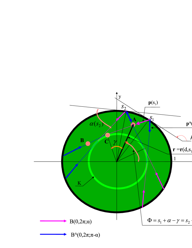
Figure 2: The two bundle $B(0,2\pi;\alpha)$ and $B^{A}(0,2\pi;\pi-\alpha),\;0<\alpha,$ of the skeleton B in the circular billiards

For these two bundles the corresponding SWF’s are the following (see Fig.2):

$$\Psi^{\pm}(d,s,\lambda)=(d-\sin\alpha)^{-\frac{1}{2}}e^{\pm i\lambda p(d\pm s\cos\alpha)}\chi^{\pm}(d,s,\lambda)$$

$$\Psi_{A}^{\pm}(d,s,\lambda)=(d-\sin\alpha)^{-\frac{1}{2}}e^{\pm i\lambda p(d\mp s\cos\alpha)}\chi_{A}^{\pm}(d,s,\lambda)$$ (50)

The above SWF’s are defined in the ring $0\leq d<\sin\alpha,\;0\leq s\leq 2\pi$ of the circular billiards.

Since both the bundles are defined in the ring mentioned the SWF’s have to satisfy the following uniqueness conditions:

$$\Psi^{\pm}(d,s,\lambda)=\Psi^{\pm}(d,s+2\pi,\lambda)$$

$$\Psi_{A}^{\pm}(d,s,\lambda)=\Psi_{A}^{\pm}(d,s+2\pi,\lambda)$$ (51)

which lead to

$$\lambda p\cos\alpha=-\lambda p\cos(\pi-\alpha)=m,\;\;\;\;\;\;\;\;m=0,\pm 1,\pm 2,...$$ (52)

and means the angular momentum quantization together with

$$\chi^{\pm}(d,s+2\pi,\lambda)=\chi^{\pm}(d,s,\lambda)$$

$$\chi_{A}^{\pm}(d,s+2\pi,\lambda)=\chi_{A}^{\pm}(d,s,\lambda)$$ (53)

We can demand from the SWF’s $\Psi^{\pm}(d,s,\lambda)$ and $\Psi_{A}^{\pm}(d,s,\lambda)$ to be eigenfunctions $\Psi_{\pm m}(d,s,\lambda)$ ($=\Psi^{\pm}(d,s,\lambda)$) and $\Psi_{A;\pm m}(d,s,\lambda)$ ($=\Psi_{A}^{\mp}(d,s,\lambda)$) of the respective angular momenta $\pm m\hbar$, $m=0,1,2,...$, where $m=\lambda p\cos\alpha$. Then it follows easily from the forms of the SWF’s considered that for the corresponding $\chi_{\pm m}(d,s,\lambda)$ and $\chi_{A;\pm m}(d,s,\lambda)$ we have to have:

$$\frac{\partial\chi_{\pm m}(d,s,\lambda)}{\partial s}=\frac{\partial\chi_{A;\pm m}(d,s,\lambda)}{\partial s}=0$$ (54)

i.e. both $\chi_{\pm m}(d,s,\lambda)$ and $\chi_{A;\pm m}(d,s,\lambda)$ are independent of $s$ and therefore they are constant on the circle boundary, i.e. for $d=0$.

Putting therefore $\chi_{m}^{\pm}(0,s,\lambda)\equiv 1$ and assuming further the following boundary conditions:

$$\chi_{\pm m}(0,s,\lambda)=-\chi_{A;\pm m}(0,s,\lambda)\equiv 1$$ (55)

we get for the appropriate $\Psi_{\pm m}^{as}(x,y,\lambda)$ vanishing on the circle boundary and being the angular momentum eigenfunction:

$$\Psi_{\pm m}^{as}(x,y,\lambda)=\Psi_{\pm m}(d,s_{1},\lambda)+\Psi_{A;\pm m}(d,s_{2},\lambda)$$

$$m=0,1,2,...$$

$$(x,y)=(\cos s_{1},\sin s_{1})+d(-\sin(\alpha+s_{1}),\cos(\alpha+s_{1}))=$$

$$(\cos s_{2},\sin s_{2})-d(-\sin(-\alpha+s_{2}),\cos(-\alpha+s_{2}))$$ (56)

Making further the identification

$$\Psi_{A;\pm m}(d,s,\lambda)=\Psi_{\pm m}^{cont}(2\sin\alpha-d,s-2\alpha,\lambda),\;\;\;\;\sin\alpha>d\geq 0$$ (57)

where $\Psi_{\pm m}^{cont}(d,s,\lambda)$ denote $\Psi_{\pm m}(d,s,\lambda)$ continued by the caustic $r=\cos\alpha$ we get for $\Psi_{\pm m}^{as}(x,y,\lambda)\equiv\Psi_{\pm m}^{as}(r\cos\Phi,r\sin\Phi,\lambda)$ (see Fig.2):

$$\Psi_{\pm m}^{as}(r\cos\Phi,r\sin\Phi,\lambda)=\Psi_{\pm m}(d,s,\lambda)+\Psi_{A;\pm m}(d,2\Phi-s,\lambda)=$$

$$\Psi_{\pm m}(d,s,\lambda)+\Psi_{\pm m}^{cont}(2\sin\alpha-d,2\Phi-s-2\alpha,\lambda)=$$

$$(\sin\alpha-d)^{-\frac{1}{2}}\left(-ie^{\pm i\lambda pd\pm ims}\chi_{\pm m}(d,s,\lambda)\right.\pm$$

$$\left.e^{\mp i\lambda p(d-2\sin\alpha)\pm im(2\Phi-s-2\alpha)}\chi_{\pm m}^{cont}(2\sin\alpha-d,2\Phi-s-2\alpha,\lambda)\right)=$$

$$m=0,1,2,...$$

$$d=\sin\alpha-\sqrt{r^{2}-\cos^{2}\alpha}$$

$$\sin(\Phi-s)=\frac{\sin\alpha}{r}(\sin\alpha-\sqrt{r^{2}-\cos^{2}\alpha})$$

$$\sin\alpha>d\geq 0$$ (58)

The identification conditions (57) give:

$$\chi_{A;\pm m}(d,s,\lambda)=e^{\pm 2i(\lambda p\sin\alpha-m\alpha-\frac{\pi}{4})}\chi_{\pm m}^{cont}(2\sin\alpha-d,s-2\alpha,\lambda)$$

$$\sin\alpha>d\geq 0$$ (59)

Applying now (49) and (55) we get:

$$1=e^{\pm 2i(\lambda p\sin\alpha-m\alpha+\frac{\pi}{4})}$$

$$\chi_{\pm m}^{cont}(2\sin\alpha,s-2\alpha,\lambda)=\chi_{\pm m}(0,s,\lambda)\equiv 1$$ (60)

so that

$$\int_{0}^{2\sin\alpha}\left(J^{\frac{1}{2}}\triangle\left(J^{-\frac{1}{2}}{\chi}_{\pm m;k}(a,s)\right)+2\sum_{l=0}^{k}E_{k-l+1}{\chi}_{\pm m;l}(a,s)\right)da=0$$

$$k=0,1,...$$ (61)

with

$$\chi_{\pm m;0}(d,s)\equiv 1$$

$$\chi_{\pm m;k+1}(d,s)=\pm\frac{i}{2p}\int_{0}^{d}\left(J^{\frac{1}{2}}\triangle\left(J^{-\frac{1}{2}}\chi_{\pm m;k}(a,s)\right)+2\sum_{l=0}^{k}E_{k-l+1}\chi_{\pm m;l}(a,s)\right)da$$

$$k=0,1,2,...$$ (62)

The integrations in the formulae (61)-(62) go above the singular point $d=\sin\alpha$ in the $d$-plane for the plus sign and below this point for the minus one.

A simple conclusion from the quantization conditions (61)-(62) is that:

$$\left(\chi_{+m;k}(d,s)\right)^{*}=\chi_{-m;k}(d,s)$$

$$k=0,1,2,...$$ (63)

so that

$$\left(\Psi_{+m}^{as}(x,y,\lambda)\right)^{*}=\Psi_{-m}^{as}(x,y,\lambda)$$ (64)

i.e. the semiclassical energies $E$ in the circular billiards are degenerate with respect to the sign of the angular momentum.

Of course the above conclusions are well known as exact for the circular billiards.

Therefore in the equations (61)-(62) we can choose only the plus sign in the respective calculations to get:

$$\lambda\sqrt{2E_{0;mr}-\frac{m^{2}}{\lambda^{2}}}-m\arccos\frac{m}{\lambda\sqrt{2E_{0}}}=r\pi-\frac{\pi}{4}$$

$$\cos\alpha_{mr}=\frac{m}{\lambda\sqrt{2E_{0;mr}}}$$

$$m=0,1,2,...,\;\;\;\;r=1,2,...$$ (65)

for the ”classical” energy $E_{0}$ and the angle $\alpha$.

It follows from (65) that

$$E_{0;0r}=\frac{\left(r-\frac{1}{4}\right)^{2}\pi^{2}}{2\lambda^{2}}$$

$$\cos\alpha_{0r}=0$$

$$E_{0;mr}=\frac{m^{2}}{2\lambda^{2}F^{2}(\frac{r-\frac{1}{4}}{m}\pi)}$$

$$\cos\alpha_{mr}=F(\frac{r-\frac{1}{4}}{m}\pi)$$

$$m=1,2,...,\;\;\;\;r=1,2,...$$ (66)

where $F^{-1}(x)=(\sqrt{1-x^{2}}-x\arccos x)x^{-1},\;0<x\leq 1$.

The next to zero order terms of the corresponding semiclassical expansions can be obtained using the results of App.D from which it follows (the formulae (77)-(79)) that the operator $D(t,s)=J^{\frac{1}{2}}\cdot\triangle\cdot J^{-\frac{1}{2}}$ in (68) is bilinear in $\frac{\partial}{\partial t}$ and $\frac{\partial}{\partial s}$ with coefficients completely independent of $s$ and it acts in (68) also on the $s$-independent quantities. In such cases its action is reduced to (for $t\to x=pt$):

$$\left[J^{\frac{1}{2}}\cdot\triangle\cdot J^{-\frac{1}{2}}\right]_{red}(x,\frac{\partial}{\partial x})=$$

$$\left(\frac{\cos^{2}\alpha}{J^{2}}+1\right)\frac{\partial^{2}}{\partial x^{2}}+\frac{2\cos^{2}\alpha}{J^{3}}\frac{\partial}{\partial x}+\frac{5}{4}\frac{\cos^{2}\alpha}{J^{4}}-\frac{1}{4}\frac{1}{J^{2}}$$ (67)

where $J=\sin\alpha-x$.

Taking this into account in the second of the eqs. (61) and putting there $k=0$ we get:

$$E_{1;mr}=-\frac{1}{4\sin\alpha_{mr}}\int_{0}^{2\sin\alpha_{mr}}\left(J^{\frac{1}{2}}\cdot\triangle\cdot J^{-\frac{1}{2}}\right)_{red}\cdot 1dx=\frac{1}{8\sin\alpha_{mr}}\left(\frac{5}{6}\cot^{2}\alpha_{mr}-1\right)$$ (68)

where the integration in the $x$-plane went over upper half-circle with the center at $x=\sin\alpha_{mr}$ in the clockwise direction.

Similarly for $\chi_{mr;1}(d)$ we get:

$$\chi_{mr;1}(d)=\frac{i}{2p}\int_{0}^{d}\left(\frac{5}{4}\frac{\cos^{2}\alpha_{mr}}{J_{mr}^{4}}-\frac{1}{4}\frac{1}{J_{mr}^{2}}\right)dx+\frac{i}{p}E_{1;mr}d=$$

$$-\frac{i}{2p}\left(\frac{5}{12}\frac{\cos^{2}\alpha_{mr}}{J_{mr}^{3}}-\frac{5}{12}\frac{\cos^{2}\alpha_{mr}}{\sin^{3}\alpha_{mr}}-\frac{1}{4}\frac{1}{J_{mr}}+\frac{1}{4}\frac{1}{\sin\alpha_{mr}}\right)+\frac{i}{p}E_{1;mr}d$$ (69)

where $J_{mr}=\sin\alpha_{mr}-d$.

The higher order terms of the semiclassical expansions for $E_{mr}(\lambda)$ and $\chi_{mr}(d,\lambda)$ can be obtain analogously using the recurrent equations (61)-(62).

It is to be noticed that the above calculations form a new algorithm for the semiclassical approximation method.

6 The rectangular billiards

Consider now the rectangular billiards shown in Fig.3. This billiards is the canonical example of the energy quantization problem because of its easiness to be solved by the variable separation method. According to Fig.3 the well known solution to the problem is given by the following two equations:

$$\sin(\lambda p_{x}a)=0$$

$$\sin(\lambda p_{y}b)=0$$ (70)

with $p_{x}^{2}+p_{y}^{2}=p^{2}=2E$ as the result of the following form of the energy eigenfunction:

$$\Psi(x,y)=C\sin(\lambda p_{x}x)\sin(\lambda p_{y}y)=$$

$$-\frac{C}{4}\left(e^{\lambda p_{x}x+\lambda p_{y}y}+e^{-\lambda p_{x}x-\lambda p_{y}y}-e^{\lambda p_{x}x-\lambda p_{y}y}-e^{-\lambda p_{x}x+\lambda p_{y}y}\right)$$ (71)

Of course one can always put $p_{x}=p\cos\alpha,p_{y}=p\sin\alpha$ where $\alpha,\;0<\alpha<\frac{1}{2}\pi$, is the angle the momentum $p$ is inclined to the $x$-axis.

Let us note that the cases $\alpha=0,\frac{1}{2}\pi$ are excluded by the solutions (71).

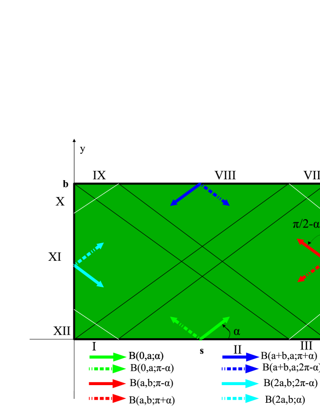
Figure 3: The rectangular billiards with eight ray bundles

6.1 The cases $0<\alpha<\frac{1}{2}\pi$

Let us consider this rectangular billiard example by the method described in the previous sections. Since the absolute values of the momentum components $p_{x},p_{y}$ are the integrals of the classical motion inside the billiards respecting elastic law of bouncing then all bundles which should be taken into account are defined by a single angle $\alpha,\;0<\alpha<\frac{1}{2}\pi$, which are made by the rays of the bundle $B_{1}=B(0,a;\alpha)$ with the $x$-axis, see Fig.3.

Choosing the case of the angle $\alpha$ shown in Fig.3 the remaining seven bundles of the skeleton B shown in Fig.3 are $B_{2}=B(0,a;\pi-\alpha),\;B_{3}=B(a,b;\pi-\alpha),\;B_{4}=B(a,b;\pi+\alpha),\;B_{5}=B(a+b,a;\pi+\alpha),\;B_{6}=B(a+b,a;2\pi-\alpha),\;B_{7}=B(2a+b,b;2\pi-\alpha),\;B_{8}=B(2a+b,b;\alpha)$, i.e. the parameter $s$ introduced in sec.3 is counted anticlockwise starting from the point $(0,0)$ of Fig.3 (and having negative value if measured clockwise). The bundles $B_{2k-1},\;B_{2k},\;k=1,...,4,$ are defined on the respective sides $L_{k},\;k=1,...,4,$ of the billiards, i.e. on $L_{1}=L(0,a),\;L_{2}=L(a,b),\;L_{3}=L(a+b,a),\;L_{4}=L(2a+b,b)$.

The skeleton ${\bf B}^{T}$ coincides exactly with B in the case of the rectangular billiards.

Let us note that a number of bundles in the skeletons is obviously independent of a choice of $\alpha$, i.e. it is always equal to eight.

Note also that unlike the circular billiard bundles the rectangular bundles do not have their caustics inside the billiards, but rather in the infinities.

The semiclassical wave function $\Psi^{as}(x,y)$ constructed according the rules discussed earlier should be the sum at most of the eight SWF’s $\Psi_{i}^{+}(d,s,\lambda),\;i=1,...,8$, which are constructed on the respective bundles $B_{i},\;i=1,...,8$, of the skeleton B. But as it follows from Fig.4 only four of them interfere in each point of the rectangular billiards, i.e. we have:

$$\Psi^{as}(x,y)=\sum_{i=1}^{8}\Psi_{i}^{+}(d_{i},s_{i},\lambda)=\sum_{i=1}^{4}\Psi_{k_{i}}^{+}(d_{i},s_{i},\lambda)$$

$$x=x_{0}(s_{i})+d_{i}\cos\alpha(s_{i})$$

$$y=y_{0}(s_{i})+d_{i}\sin\alpha(s_{i})$$

$$i=1,...,4$$ (72)

where $\alpha(s_{i})$ are the angles the rays in Fig.4 make with the $x$-axis and $(x_{0}(s_{i}),y_{0}(s_{i}))$ are the points of the rectangular boundary from which the rays start. The parameters $s_{i}$ as previously measure distances of the boundary points $(x_{0}(s_{i}),y_{0}(s_{i}))$ from the point $(0,0)$ in anticlockwise direction along the boundary. The corresponding Jamaicans are $J(t,s_{i})=\sqrt{-\sin\alpha(s_{i})}$, i.e. are constant but discontinues. Therefore they will be included into the $\chi$-factors contained in the SWF’s.

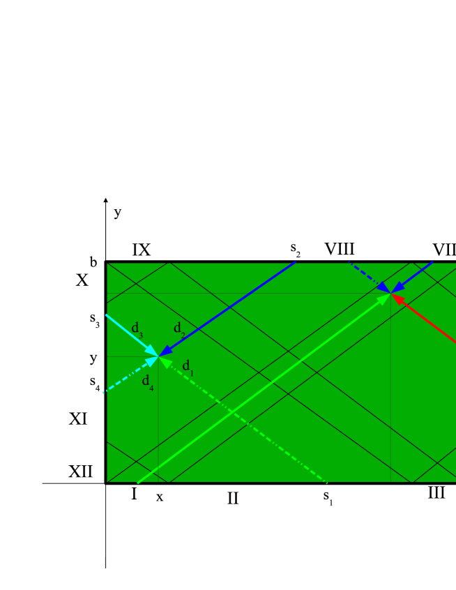
Figure 4: Four solutions $\Psi_{i}^{+}(d_{i},s_{i}),\;i=1,...,4$, meeting at the point ($x,y$)

Let us note that $\Psi^{as}(x,y)$ can be discontinue each time the point $(x,y)$ crosses the thin black lines in Fig.3. being the boundary of different bundles. Let us enumerate these lines by $l_{i},\;i=1,...,4,$ starting from the line emerging from the point $(0,0)$ and continuing anticlockwise.

It is then easy to see that to ensure the continuity of $\Psi^{as}(x,y)$ in each point in the billiards it is enough to identify the respective $\chi$-coefficients on the respective lines defining them elsewhere in the billiards as continuous functions of $s$ and $d$. We get such a continuity putting:

$$\chi_{1}^{\pm}(d,0,\lambda)=\chi_{8}^{\pm}(d,0,\lambda)$$

$$\chi_{3}^{\pm}(d,a,\lambda)=\chi_{2}^{\pm}(d,a,\lambda)$$

$$\chi_{5}^{\pm}(d,a+b,\lambda)=\chi_{4}^{\pm}(d,a+b,\lambda)$$

$$\chi_{7}^{\pm}(d,2a+b,\lambda)=\chi_{6}^{\pm}(d,2a+b,\lambda)$$ (73)

Of course $\Psi^{as}(x,y)$ vanishes on the rectangular boundary, i.e. we have to have:

$$\Psi^{as}(0,y)=\Psi^{as}(a,y)=\Psi^{as}(x,0)=\Psi^{as}(x,b)=0$$

$$0<x<a,\;\;\;0<y<b$$ (74)

The conditions (74) expressed in terms of the SWF’s $\Psi_{i}^{\pm}(d,s,\lambda),\;i=1,...,8,$ take the following detailed forms:

$$\Psi_{2k-1}^{+}(0,s,\lambda)+\Psi_{2k}^{-}(0,s,\lambda)=0$$

$$\Psi_{2k}^{+}(0,s,\lambda)+\Psi_{2k-1}^{-}(0,s,\lambda)=0$$

$$s\in L_{k},\;\;\;\;\;\;\;k=1,...,4$$ (75)

When identifying $\Psi_{i}^{-}(0,s,\lambda),\;i=1,...,8$, with the respective $\Psi_{j}^{+}(d_{j}(s),f_{j}(s),\lambda),\;j=1,...,8$, it should be noticed that for each considered trajectory family there is no caustic inside the rectangular billiards so that each integral $\int_{K}p_{x}dx+p_{y}dy$ along the close loop $K$ lying inside the billiards or on its boundary has to vanish. As a consequence of this the identifications we are talking about are then reduced just to the identifications of the corresponding $\chi$-factors, i.e the possible phase factors are factored out. Therefore we get successively for the conditions (75) to be satisfied:

1. $s>0,\;{\bf r}_{0}(s)\in I,\;-s\tan\alpha\in XII,\;2a+b-b\cot\alpha-{\bf r}_{0}(s)\in VII$

   $$\chi_{1}^{-}(0,s,\lambda)=\chi_{4}^{+}\left(\frac{b}{\sin\alpha},2a+b-b\cot\alpha-s,\lambda\right)$$

   $$\chi_{2}^{-}(0,s,\lambda)=\chi_{7}^{+}\left(\frac{s}{\cos\alpha},-s\tan\alpha,\lambda\right)$$ (76)

   and hence and from (75)

   $$\chi_{1}(0,s,\lambda)+\chi_{7}\left(\frac{s}{\cos\alpha},-s\tan\alpha,\lambda\right)=0$$

   $$\chi_{2}(0,s,\lambda)+\chi_{4}\left(\frac{b}{\sin\alpha},2a+b-b\cot\alpha-s,\lambda\right)=0$$ (77)

   In the last two equations the plus signs at $\chi_{j}^{+},\;j=1,...,8$, have been dropped and this convention will be kept in further equations if not leading to misunderstandings.

2. $s>0,\;{\bf r}_{0}(s)\in II,\;-s\tan\alpha\in X+XI,\;a+(a-s)\tan\alpha\in V+VI)$

   $$\chi_{1}^{-}(0,s,\lambda)=\chi_{4}^{+}\left(\frac{a-s}{\cos\alpha},a+(a-s)\tan\alpha,\lambda\right)$$

   $$\chi_{2}^{-}(0,s,\lambda)=\chi_{7}^{+}\left(\frac{s}{\cos\alpha},-s\tan\alpha,\lambda\right)$$ (78)

   and hence and from (75)

   $$\chi_{1}(0,s,\lambda)+\chi_{7}\left(\frac{s}{\cos\alpha},-s\tan\alpha,\lambda\right)=0$$

   $$\chi_{2}(0,s,\lambda)+\chi_{4}\left(\frac{a-s}{\cos\alpha},a+(a-s)\tan\alpha,\lambda\right)=0$$ (79)

3. ${\bf r}_{0}(s)\in III,\;s>0,\;(-b-s+b\cot\alpha\in IX,\;a+(a-s)\tan\alpha\in IV$

   $$\chi_{1}^{-}(0,s,\lambda)=\chi_{4}^{+}\left(\frac{a-s}{\cos\alpha},a+(a-s)\tan\alpha,\lambda\right)$$

   $$\chi_{2}^{-}(0,s,\lambda)=\chi_{6}^{+}\left(\frac{b}{\sin\alpha},-b-s+b\cot\alpha,\lambda\right)$$ (80)

   and hence

   $$\chi_{1}(0,s,\lambda)+\chi_{6}\left(\frac{b}{\sin\alpha},-b-s+b\cot\alpha,\lambda\right)=0$$

   $$\chi_{2}(0,s,\lambda)+\chi_{4}\left(\frac{a-s}{\cos\alpha},a+(a-s)\tan\alpha,\lambda\right)=0$$ (81)

4. $s>0,\;{\bf r}_{0}(s)\in IV+V+VI,\;a-(s-a)\cot\alpha\in II+III,\\ a+b+(a+b-s)\cot\alpha\in VII+VIII$

   $$\chi_{3}^{-}(0,s,\lambda)=\chi_{6}^{+}\left(\frac{a+b-s}{\sin\alpha},a+b+(a+b-s)\cot\alpha,\lambda\right)$$

   $$\chi_{4}^{-}(0,s,\lambda)=\chi_{1}^{+}\left(\frac{s-a}{\sin\alpha},a-(s-a)\cot\alpha,\lambda\right)$$ (82)

   and hence

   $$\chi_{3}(0,s)e^{-i\lambda pa\cos\alpha}+\chi_{1}\left(\frac{s-a}{\sin\alpha},a-(s-a)\cot\alpha,\lambda\right)e^{i\lambda pa\cos\alpha}=0$$

   $$\chi_{4}(0,s,\lambda)e^{-i\lambda pa\cos\alpha}+\chi_{6}\left(\frac{a+b-s}{\sin\alpha},a+b+(a+b-s)\cot\alpha,\lambda\right)e^{i\lambda pa\cos\alpha}=0$$ (83)

5. $s>0,\;{\bf r}_{0}(s)\in VII,\;2a+b-b\cot\alpha-{\bf r}_{0}(s)\in I,\;a+b-(s-a-b)\tan\alpha\in VI$

   $$\chi_{5}^{-}(0,s,\lambda)=\chi_{1}^{+}\left(\frac{b}{\sin\alpha},2a+b-b\cot\alpha-s,\lambda\right)$$

   $$\chi_{6}^{-}(0,s,\lambda)=\chi_{3}^{+}\left(\frac{s-a-b}{\cos\alpha},a+b-(s-a-b)\tan\alpha,\lambda\right)$$ (84)

   and hence

   $$\chi_{6}(0,s,\lambda)e^{-i\lambda pb\sin\alpha}+\chi_{1}\left(\frac{b}{\sin\alpha},2a+b-b\cot\alpha-s,\lambda\right)e^{i\lambda pb\sin\alpha}=0$$

   $$\chi_{5}(0,s,\lambda)e^{-i\lambda pb\sin\alpha}+\chi_{3}\left(\frac{s-a-b}{\cos\alpha},a+b-(s-a-b)\tan\alpha,\lambda\right)e^{i\lambda pb\sin\alpha}=0$$ (85)

6. $s<0,\;{\bf r}_{0}(s)\in VIII,\;-b-(b+s)\tan\alpha\in X+XI+XII,\\ a+b-(a+b+s)\tan\alpha\in IV+V$

   $$\chi_{3}^{-}(0,s)=\chi_{1}^{+}\left(\frac{-b-s}{\cos\alpha},-b-(b+s)\tan\alpha,\lambda\right)$$

   $$\chi_{4}^{-}(0,s)=\chi_{2}^{+}\left(\frac{a+b+s}{\cos\alpha},a+b-(a+b+s)\tan\alpha,\lambda\right)$$ (86)

   and hence

   $$\chi_{4}(0,s,\lambda)e^{-i\lambda pb\sin\alpha}+\chi_{1}\left(\frac{-b-s}{\cos\alpha},-b-(b+s)\tan\alpha,\lambda\right)e^{+i\lambda pb\sin\alpha}=0$$

   $$\chi_{3}(0,s,\lambda)e^{-i\lambda pb\sin\alpha}+\chi_{2}\left(\frac{a+b+s}{\cos\alpha},a+b-(a+b+s)\tan\alpha,\lambda\right)e^{i\lambda pb\sin\alpha}=0$$ (87)

7. $s<0,\;{\bf r}_{0}(s)\in IX,\;-b-(b+s)\tan\alpha\in X,\;b\cot\alpha-b-{\bf r}_{0}(s)\in III$

   $$\chi_{5}^{-}(0,s)=\chi_{8}^{+}\left(\frac{-b-s}{\cos\alpha},-b-(b+s)\tan\alpha,\lambda\right)$$

   $$\chi_{6}^{-}(0,s)=\chi_{2}^{+}\left(\frac{b}{\sin\alpha},b\cot\alpha-b-s,\lambda\right)$$ (88)

   and hence

   $$\chi_{6}(0,s,\lambda)e^{-i\lambda pb\sin\alpha}+\chi_{8}\left(\frac{-b-s}{\cos\alpha},-b-(b+s)\tan\alpha,\lambda\right)e^{+i\lambda pb\sin\alpha}=0$$

   $$\chi_{5}(0,s,\lambda)e^{-i\lambda pb\sin\alpha}+\chi_{2}\left(\frac{b}{\sin\alpha},b\cot\alpha-b-s,\lambda\right)e^{i\lambda pb\sin\alpha}=0$$ (89)

8. $s<0,\;{\bf r}_{0}(s)\in X+XI+XII,\;-s\cot\alpha\in I+II,\\ -b-(s+b)\cot\alpha\in VIII+IX$

   $$\chi_{8}^{-}(0,s,\lambda)=\chi_{5}^{+}\left(\frac{b+s}{\sin\alpha},-b-(s+b)\cot\alpha,\lambda\right)$$

   $$\chi_{7}^{-}(0,s,\lambda)=\chi_{2}^{+}\left(\frac{-s}{\sin\alpha},-s\cot\alpha,\lambda\right)$$ (90)

   and hence

   $$\chi_{7}(0,s,\lambda)+\chi_{2}\left(\frac{-s}{\sin\alpha},-s\cot\alpha,\lambda\right)=0$$

   $$\chi_{8}(0,s,\lambda)+\chi_{3}\left(\frac{b+s}{\sin\alpha},-b-(s+b)\cot\alpha,\lambda\right)=0$$ (91)

Solving the last set of the quantization conditions we should get the solutions for the energy levels and for the corresponding $\Psi^{as}(x,y)$.

However the above conditions do not provide us with the solutions for $\chi_{i}(0,s,\lambda),\;i=1,...,8$, in some algebraic forms. Rather they show how a solution defined on some bundle propagates along its rays to be transformed by bouncing off the rectangular boundary into another bundle and finally after a finite number of such bouncings achieving its mother bundle and repeating this process infinitely.

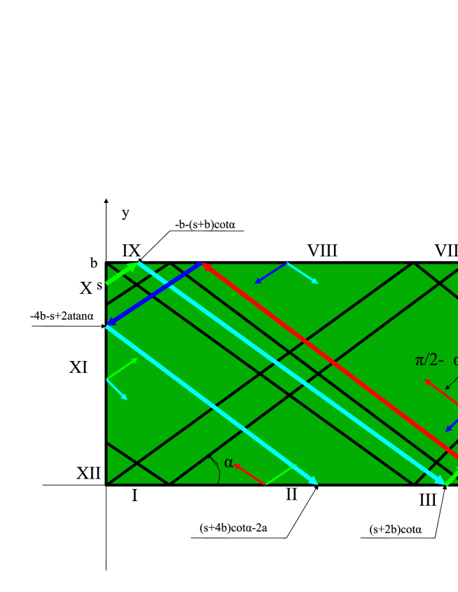
Figure 5: The solution $\Psi_{8}^{+}(t,s)$ being carried by the successive bundles $B_{8}\to B_{6}\to B_{1}\to B_{3}\to B_{5}\to B_{7}\to B_{1}$

To get a knowledge what really happens by such bouncings consider for example the green color ray along which the solution $\Psi_{8}^{+}(t,s)$ propagates, shown in Fig.5 emerging from the point $s,\;{\bf r}_{0}(s)\in X$, of the rectangular boundary. This particular ray bounces into the blue-light one and next again into the green one. Taking into account first the conditions (85) and next (81) we get:

$$\chi_{1}(0,(s+2b)\cot\alpha,\lambda)=-\chi_{6}\left(\frac{b}{\sin\alpha},-b-(s+b)\cot\alpha,\lambda\right)=$$

$$\chi_{8}^{cont}\left(\frac{2b+s}{\sin\alpha},s,\lambda\right)e^{+2i\lambda pb\sin\alpha},\;\;\;\;\;{\bf r}_{0}(s)\in X$$ (92)

and continuing the bounces to achieve the green ray again we get:

$$\chi_{1}(0,(s+4b)\cot\alpha-2a,\lambda)=\chi_{8}^{cont}(D(s),s,\lambda)e^{4i\lambda pb\sin\alpha+2i\lambda pa\cos\alpha},\;\;\;\;\;{\bf r}_{0}(s)\in X$$ (93)

where $D(s)$ is the total distance the green ray has passed from the point $s$ to the point $(s+4b)\cot\alpha-2a$ bouncing multiply from the boundary.

But taking into account the first of the identification (73) and the identification (49) we have to have:

$$\chi_{1}(0,(s+2b)\cot\alpha,\lambda)=\chi_{8}^{cont}\left(\frac{2b+s}{\sin\alpha},s,\lambda\right)$$

$$\chi_{1}(0,(s+4b)\cot\alpha-2a,\lambda)=\chi_{8}^{cont}(D(s),s,\lambda)$$

$${\bf r}_{0}(s)\in X$$ (94)

so that

$$e^{+2i\lambda pb\sin\alpha}=1$$

$$e^{4i\lambda pb\sin\alpha+2i\lambda pa\cos\alpha}=1$$ (95)

and consequently:

$$\lambda pb\sin\alpha=m\pi$$

$$\lambda pa\cos\alpha=n\pi$$

$$m,n=1,2,...$$ (96)

Taking the limit $\lambda\to\infty$ in (94) we get:

$$\chi_{1,0}((s+2b)\cot\alpha)=\chi_{1,0}((s+4b)\cot\alpha-2a)=\chi_{8,0}(s)$$ (97)

If $\tan\alpha=\frac{m}{n}\frac{a}{b}$ is not rational none of the arrival points can be repeated, i.e. the corresponding trajectory is not closed (periodic), and the (infinite) set of such points is dense on the side $L_{1}$ of the billiards. Therefore the equations (97) show that $\chi_{1,0}(s)$ has to be not only a constant of motion but also $s$-independent since this equation can be written in infinitely many points of $L_{1}$ densely distributed on it.

The last conclusion is valid also of course for the remaining $\chi_{k,0}(s),\;k=1,...,8,$ and as it can be easily concluded from (14) and App.D all the coefficients $\chi_{k}(d,s,\lambda),\;k=1,...,8,$ are then also constant. Putting therefore $\chi_{1}(d,s,\lambda)\equiv 1$ we get by (73) and (75):

$$\chi_{k}(d,s,\lambda)\equiv 1,\;\;\;\;\;\;\;k=1,4,5,8$$

$$\chi_{k}(d,s,\lambda)\equiv-1,\;\;\;\;\;\;\;k=2,3,6,7$$ (98)

Choosing therefore the point $(x,y)$ of Fig.4 for the SWF (72) we get:

$$\Psi^{as}(x,y)=\Psi_{2}^{+}(d_{1},s_{1})+\Psi_{5}^{+}(d_{2},s_{2})+\Psi_{7}^{+}(d_{3},s_{3})+\Psi_{8}^{+}(d_{4},s_{4})=$$

$$\sum_{l=1}^{4}(-1)^{l}e^{i\lambda p^{2}t_{l}+i\lambda pf_{l}(s_{l})}$$ (99)

where $t_{l}$ and $f_{l}(s_{l}),\;l=1,...,4$ should be calculated from the relations (see Fig.5):

$$x=x_{0}(s_{l})+pt_{l}\cos\alpha(s_{l})$$

$$y=y_{0}(s_{l})+pt_{l}\sin\alpha(s_{l})$$

$$\alpha(s_{l})=\alpha,\;\frac{1}{2}\pi-\alpha$$ (100)

However making use of the independence of the phase integral $\int_{(0,0)}^{(x,y)}p_{x}dx+p_{y}dy$ of the integration paths we get for the particular terms in the sum in (99):

$$e^{i\lambda p^{2}t_{1}+i\lambda pf_{1}(s_{1})}=e^{i\lambda(-p_{x}x+p_{y}y)}$$

$$e^{i\lambda p^{2}t_{2}+i\lambda pf_{2}(s_{2})}=e^{i\lambda(-p_{x}x-p_{y}y)}$$

$$e^{i\lambda p^{2}t_{3}+i\lambda pf_{3}(s_{3})}=e^{i\lambda(p_{x}x-p_{y}y)}$$

$$e^{i\lambda p^{2}t_{4}+i\lambda pf_{4}(s_{4})}=e^{i\lambda(p_{x}x+p_{y}y)}$$ (101)

and finally:

$$\Psi^{as}(x,y)=-e^{i\lambda(-p_{x}x+p_{y}y)}+e^{i\lambda(-p_{x}x-p_{y}y)}-e^{i\lambda(p_{x}x-p_{y}y)}+e^{i\lambda(p_{x}x+p_{y}y)}=$$

$$-4\sin(p_{x}x)\sin(p_{y}y)$$ (102)

reproducing in this way the exact result (71).

The cases when $\tan\alpha=\frac{m}{n}\frac{a}{b}$ is rational are possible only if $\frac{a}{b}$ is rational. For maintaining the results for the irrational $\frac{a}{b}$ one can argue relying on a continuity of all the investigated quantities considered as functions of $a,b$, since each point $(a,b)$ with rational value of $\frac{a}{b}$ is densely surrounded by the ones for which $\frac{a}{b}$ is irrational.

6.2 The cases $\alpha=0,\;\frac{1}{2}\pi$ - the bouncing mode skeletons

It is surprising that the cases $\alpha=0,\;\frac{1}{2}\pi$ are not allowed by the representation (71) of the SWF leading to the totally vanishing solutions while there are still the bundle skeletons with these angles on which non vanishing identically SWF’s can be constructed. Therefore we should get some new knowledge about the semiclasscical method developed here considering these cases known as the bouncing modes.

Consider the case $\alpha=\frac{1}{2}\pi$. The second case will be analogous.

There are two bundles in this case which the skeleton ${\bf B}$ is consisting of. The one $B_{1}$ with its rays directed up and starting from the side $L_{1}$ and the second $B_{3}$ with rays directed down starting from the side $L_{3}$ (Fig.6). The skeleton ${\bf B}^{A}$ is identical with ${\bf B}$.

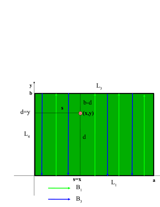
Figure 6: The two bouncing mode bundles $B_{1}$ and $B_{3}$ of the vertical skeleton in the rectangular billiards

For these particular cases of bundles rays for both the bundles will be positioned by the same parameter $s$ measuring a distance of a ray from the $y$-axis along the corresponding sides $L_{1}$ and $L_{3}$. Therefore for the corresponding SWF’s we get:

$$\Psi_{1}^{\pm}(d,s,\lambda)=e^{\pm i\lambda pd}\chi_{1}^{\pm}(d,s,\lambda)$$

$$\Psi_{3}^{\pm}(b-d,s,\lambda)=e^{\pm i\lambda p(b-d)}\chi_{3}^{\pm}(b-d,s,\lambda)$$

$$0\leq d\leq b,\;\;\;\;0<s<a$$ (103)

For the SWF $\Psi^{as}(x,y,\lambda)$ we have:

$$\Psi^{as}(x,y,\lambda)=\Psi_{1}^{+}(d,s,\lambda)+\Psi_{3}^{+}(b-d,s,\lambda)=\Psi_{1}^{-}(b-d,s,\lambda)+\Psi_{3}^{-}(d,s,\lambda)$$

$$(x,y)=(s,d)$$ (104)

together with the following identifications:

$$\Psi_{3}^{\pm}(b-d,s,\lambda)=\Psi_{1}^{\mp}(d,s,\lambda)$$

$$\Psi_{1}^{+}(0,s,\lambda)=-\Psi_{1}^{-}(0,s,\lambda)$$

$$\Psi_{3}^{+}(0,s,\lambda)=-\Psi_{3}^{-}(0,s,\lambda)$$ (105)

so that:

$$\chi_{3}^{\pm}(b-d,s,\lambda)=e^{\mp i\lambda pb}\chi_{1}^{\mp}(d,s,\lambda)$$

$$\chi_{1}^{+}(0,s,\lambda)=-\chi_{1}^{-}(0,s,\lambda)$$

$$\chi_{3}^{+}(0,s,\lambda)=-\chi_{3}^{-}(0,s,\lambda)$$ (106)

It follows from the last equations that:

$$\chi_{3}^{+}(0,s,\lambda)=-\chi_{3}^{-}(0,s,\lambda)=-e^{i\lambda pb}\chi_{1}^{+}(b,s,\lambda)$$ (107)

so that:

$$\chi_{3}^{+}(b,s,\lambda)=-e^{i\lambda pb}\chi_{1}^{+}(2b,s,\lambda)$$ (108)

and further:

$$\chi_{1}^{+}(0,s,\lambda)=-\chi_{1}^{-}(0,s,\lambda)=-e^{i\lambda pb}\chi_{3}^{+}(b,s,\lambda)=e^{2i\lambda pb}\chi_{1}^{+}(2b,s,\lambda)=e^{2i\lambda pb}\chi_{1}^{+}(0,s,\lambda)$$ (109)

since $\chi_{1}^{+}(2b,s,\lambda)=\chi_{1}^{+,cont}(0,s,\lambda)=\chi_{1}^{+}(0,s,\lambda)$.

Therefore:

$$e^{2i\lambda pb}=1$$ (110)

and

$$\Psi^{as}(x,y,\lambda)=e^{i\lambda pd}\chi_{1}^{+}(d,s,\lambda)+e^{-i\lambda pd}e^{i\lambda pb}\chi_{3}^{+}(b-d,s,\lambda)=$$

$$e^{i\lambda pd}\chi_{1}^{+}(d,s,\lambda)-e^{-i\lambda pd}\chi_{1}^{+}(2b-d,s,\lambda)$$ (111)

We have of course $\Psi^{as}(x,0,\lambda)=\Psi^{as}(x,b,\lambda)=0$ by construction. But we have to have also $\Psi^{as}(0,y,\lambda)=\Psi^{as}(a,y,\lambda)=0$, i.e. we have to have:

$$e^{i\lambda pd}\chi_{1}^{+}(d,0,\lambda)-e^{-i\lambda pd}\chi_{1}^{+}(2b-d,0,\lambda)=0$$

$$e^{i\lambda pd}\chi_{1}^{+}(d,a,\lambda)-e^{-i\lambda pd}\chi_{1}^{+}(2b-d,a,\lambda)=0$$ (112)

Therefore from (112) in the limit $\lambda\to\infty$ we have:

$$e^{i\lambda pd}\chi_{1,0}^{+}(0)-e^{-i\lambda pd}\chi_{1,0}^{+}(0)=0$$

$$e^{i\lambda pd}\chi_{1,0}^{+}(a)-e^{-i\lambda pd}\chi_{1,0}^{+}(a)=0$$ (113)

so that

$$\chi_{1,0}^{+}(0)=\chi_{1,0}^{+}(a)=0$$ (114)

Next let us invoke the second of the equations (14) to get in the considered case for $d=2b$:

$$\chi_{1,1}^{+}(2b,s)=\chi_{1,1}^{+}(0,s)+i\frac{b}{p}\left(\frac{d^{2}\chi_{1,0}^{+}(s)}{ds^{2}}+2E_{1}\chi_{1,0}^{+}(s)\right)$$ (115)

so that

$$\frac{d^{2}\chi_{1,0}^{+}(s)}{ds^{2}}+2E_{1}\chi_{1,0}^{+}(s)=0$$ (116)

since $\chi_{1,1}^{+}(2b,s)=\chi_{1,1}^{+}(0,s)$.

The obvious solution of the last equation satisfying the boundary conditions (114) is:

$$\chi_{1,0}^{+}(s)=A_{0}\sin(\sqrt{2E_{1}}s)$$

$$\sqrt{2E_{1}}a=m\pi,\;\;\;\;\;m=1,2,...$$ (117)

Coming back to the second of the equations (14) we can conclude that $\chi_{1,1}^{+}(d,s)$ again is independent of $d$. Passing next to the third of the equations (14) and repeating arguments similar to those which led us to (115)-(116) we get the following explicit dependence of $\chi_{1,1}^{+}(s)$ on $s$:

$$\chi_{1,1}^{+}(s)=A_{1}\sin(\sqrt{2E_{1}}s)+B_{1}\cos(\sqrt{2E_{1}}s)+\frac{E_{2}A_{0}s}{\sqrt{2E_{1}}}\cos(\sqrt{2E_{1}}s)$$ (118)

The boundary conditions $\chi_{1,1}^{+}(0)=\chi_{1,1}^{+}(a)=0$ enforce however $B_{1}=E_{2}=0$.

Using again (14) and the inductive arguments we come to the conclusion that $\chi_{1}^{+}(d,s,\lambda)$ is $d$-independent and coefficients of its semiclassical series have the form:

$$\chi_{1,k}^{+}(s)=A_{k}\sin(\sqrt{2E_{1}}s),\;\;\;\;\;\;k=0,1,...$$ (119)

so is the form of $\chi_{1}^{+}(s,\lambda)$ itself, i.e.

$$\chi_{1}^{+}(s,\lambda)=A(\lambda)\sin(\sqrt{2E_{1}}s)$$ (120)

Therefore coming back to (111) we get:

$$\Psi^{as}(x,y,\lambda)=(e^{i\lambda pd}-e^{-i\lambda pd})\chi_{1}^{+}(s,\lambda)=2iA(\lambda)\sin(\lambda pd)\sin(\sqrt{2E_{1}}s)$$ (121)

which again is the result of the previous way of the rectangular billiard energy quantization.

But now the energy $E$ is given by the (finite) semiclassical series:

$$E=\frac{1}{2}p^{2}+\frac{E_{1}}{\lambda^{2}}=\frac{1}{2}\left(\left(\frac{n\pi}{\lambda b}\right)^{2}+\left(\frac{m\pi}{\lambda a}\right)^{2}\right),\;\;\;\;\;m,n=1,2,...$$ (122)

Therefore we get a surprising result that SWF’s in the rectangular billiards can be built equivalently by the following two ways:

1. on the skeletons which rays are inclined to the billiard sides with corresponding angles defined by the quantization conditions (95) - in this case the $\chi$-coefficients of the SWF’s are simply constant on the rectangular boundary;

2. on one of the two skeletons which rays are perpendicular to one of the rectangular sides - in this case the corresponding $\chi$-coefficients vary along the sides perpendicular to the rays and vanish on the sides parallel to them.

But a more important conclusion which follows from the results got in this section is that a relation between the form of skeletons and the SWF’s and the corresponding energy spectrum which seemed to be suggested by the first part of the section is rather illusory since a full description of these quantities can be also obtained using a single skeleton only at least in the case of the rectangular billiards.

6.3 Broken rectangular billiards

By a broken rectangular billiards we understand the one on Fig.7, i.e. with some number of rectangular bays and peninsulas.

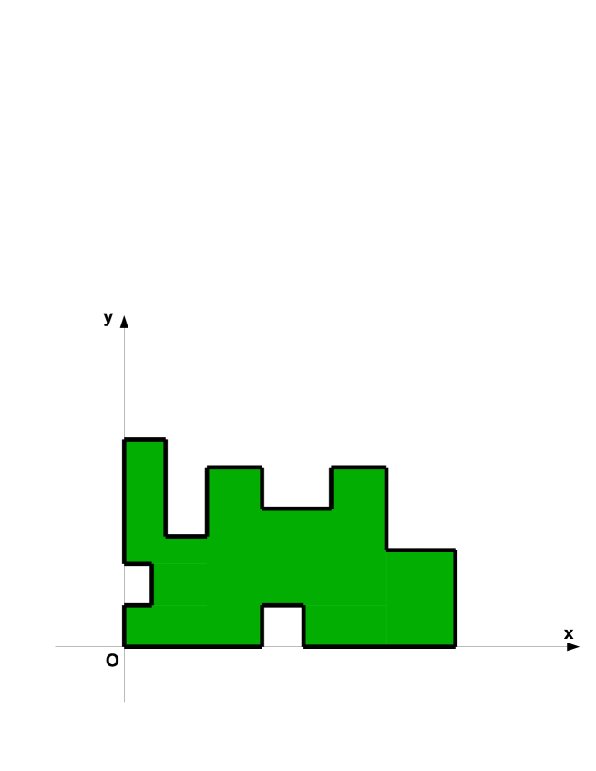
Figure 7: An ”arbitrary” broken rectangular billiards

To illustrate the way of energy quantization in such billiards we shall consider first the one with a single peninsula shown in Fig.8. The corresponding procedures are analogous to the previous ones. One needs to construct additional four bundles relating with the peninsula sides.

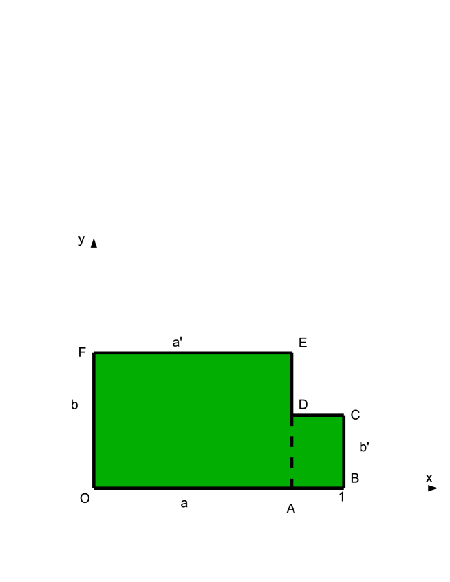
Figure 8: A single bay rectangular billiards

Although both the previous methods of the sections 5.1 and 5.2 are equivalent leading us to the same results the method of sec.5.2 seems however to be simpler and more instructive in applications to more complicated cases of billiards.

We assume from the very beginning that all the sides of the billiards from Fig.10, i.e. $a=1,b,a^{\prime},b^{\prime}$ are commensurate. This assumption can always be satisfied even if the sides are expressed by irrational number just by respective approximations of the latter by rational ones with arbitrary accuracies. We proceed as follows.

We construct two vertical skeletons. One for the rectangle $OAEF$ and the second for $ABCD$.

For the first skeleton according to (121) we get the following SWF:

$$\Psi_{1}^{as}(x,y,\lambda)=A_{1}\sin(\lambda py)\sin(\sqrt{2E_{1}}x)$$

$$0\leq x<a^{\prime},\;0\leq y\leq b$$

$$\lambda pb=m\pi,\;\;\;\;\;m=1,2,...$$

$$\sqrt{2E_{1}}a^{\prime}=n\pi,\;\;\;\;\;n=1,2,...$$ (123)

while for the second:

$$\Psi_{2}^{as}(x,y,\lambda)=A_{2}\sin(\lambda p^{\prime}y^{\prime})\sin\left(\sqrt{2E_{1}^{\prime}}(1-x^{\prime})\right)$$

$$a^{\prime}<x^{\prime}\leq 1,\;0\leq y^{\prime}\leq b^{\prime}$$

$$\lambda p^{\prime}b^{\prime}=k\pi,\;\;\;\;\;k=1,2,...$$ (124)

To get $\Psi_{2}^{as}(x,y,\lambda)$ for the total rectangular we have to match both the previous ones on the segment $AD$ of Fig.8. Since this matching has to be valid for $0\leq y^{\prime}\leq b^{\prime}$ then as it follows easily we have to have $p=p^{\prime}$ so that $E_{1}=E_{1}^{\prime}$ because of (122), i.e. the vertical wave lengths of both the matched solutions have to be the same. Therefore we get:

$$A_{1}\sin(\sqrt{2E_{1}}a^{\prime})=A_{2}\sin\left(\sqrt{2E_{1}}(1-a^{\prime})\right)$$

$$A_{1}\cos(\sqrt{2E_{1}}a^{\prime})=-A_{2}\cos\left(\sqrt{2E_{1}}(1-a^{\prime})\right)$$ (125)

so that $\sqrt{2E_{1}}=l\pi,\;l=1,2,...,$ and $A_{2}=(-1)^{l+1}A_{1}$.

Therefore the procedure leads us to the following quantization conditions for the energy $E_{nm}$:

$$\frac{1}{n_{0}}=n\frac{\Lambda_{x}}{2},\;\;\;\;\;\;\;\;\frac{b}{m_{0}}=m\frac{\Lambda_{y}}{2}$$

$$\Lambda_{x}=\frac{2\pi}{\sqrt{2E_{1}}},\;\;\;\;\;\;\;\;\Lambda_{y}=\frac{2\pi}{\lambda p}$$

$$E_{nm}=\frac{1}{2}p^{2}+\frac{2E}{\lambda^{2}}=\frac{2\pi^{2}}{\lambda^{2}}\left(\frac{1}{\Lambda_{x}^{2}}+\frac{1}{\Lambda_{y}^{2}}\right)=\frac{\pi^{2}}{2\lambda^{2}}\left(n^{2}n_{0}^{2}+\frac{m^{2}m_{0}^{2}}{b^{2}}\right)$$

$$m,n=1,2,...$$ (126)

where $\Lambda_{x},\;\Lambda_{y}$ are the wave lengths of rays in the horizontal and vertical skeletons respectively and $n_{0},m_{0}$ are the smallest integers satisfying $l_{0}=n_{0}a^{\prime}$ and $k_{0}b=m_{0}b^{\prime}$ where $l_{0},k_{0}$ are also integers.

The respective SWF’s are the following:

$$\Psi_{nm}^{as}(x,y,\lambda)=\left\{\begin{array}[]{lr}A\sin\frac{2\pi x}{\Lambda_{x}}\sin\frac{2\pi y}{\Lambda_{y}}=A\sin(nn_{0}\pi x)\sin\left(\frac{mm_{0}}{b}y\right)&\;\;\;\;\;\;(x,y)\in D_{br}\\ 0&\;\;\;\;\;\;(x,y)\notin D_{br}\end{array}\right.$$ (129)

where $D_{br}$ denotes the domain of the $x,y$-plane occupied by the broken rectangular of Fig.8.

One can easily realize that the last results can be easily generalized to any broken rectangular billiards. A little bit surprising is that the formulae (126) for the energy and (129) for the wave functions remain unchanged for any such a billiards while a number of conditions the wave lengths $\Lambda_{x}$ and $\Lambda_{y}$ have to satisfy filling the vertical and horizontal skeletons by integer numbers of their halves is increasing respectively to numbers of bays and peninsulas forming the sides od such billiards.

7 The simplest SWF’s solutions for polygons and Bunimovich billiards

The semiclassical quantization of the rectangular billiards in sec.5.2 shows that it is possible to quantize semiclassically in the similar way some specific configurations of the SWF’s in more complicated billiards also classically chaotic such as polygons or Bunimovich billiards. Such easy opportunities appear if billiards to be considered possess boundaries which allow us for easy constructions of corresponding skeletons. Some simple examples of such billiards are provided by a parallelogram, a trapezium, a pentagon shown in Fig.9

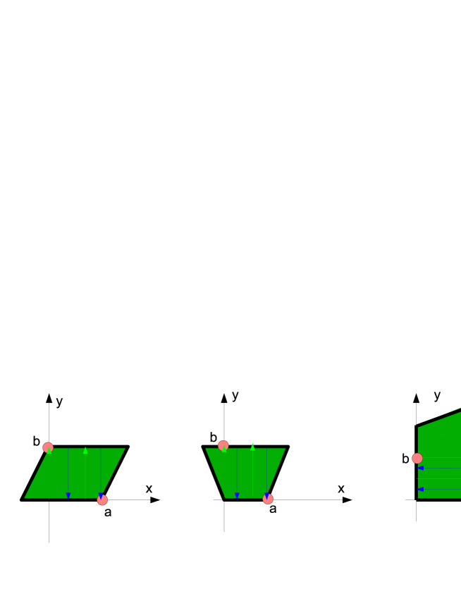
Figure 9: A parallelogram, a trapezium and a pentagon billiards with the bouncing mode skeletons

or by the Bunimovich stadium - Fig.10,

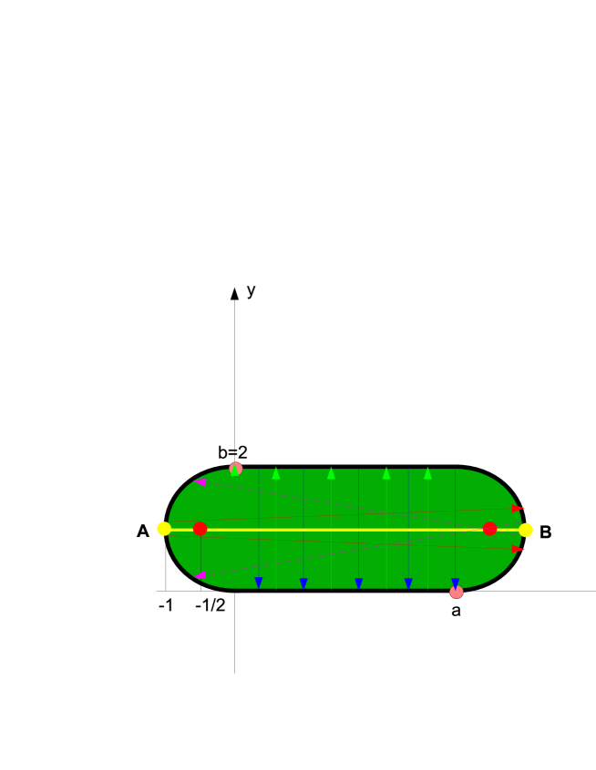
Figure 10: The Bunimovich billiards with the bouncing mode skeleton and with the scar generating bundles associated with the horizontal periodic orbit

and its simple generalizations - Fig.11.

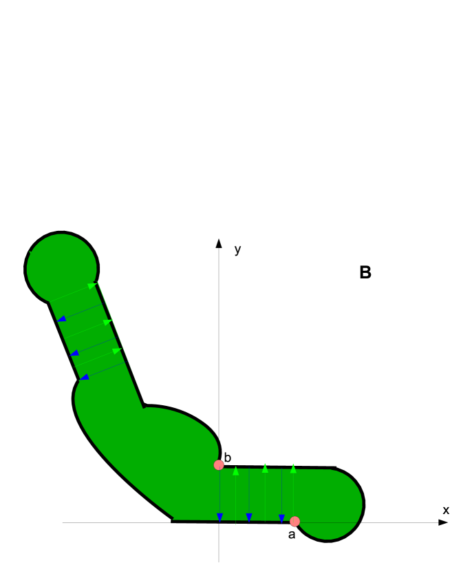
Figure 11: A simple generalization of the Bunimovich billiards with the corresponding bouncing mode skeletons

The corresponding bundle skeletons are shown on the respective figures.

The constructions of the SWF’s corresponding to the skeletons shown on the figures coincide with those for the rectangular billiards and therefore these SWF’s are the following:

$$\Psi^{as,+}(x,y,\lambda)=A\sin(\lambda p_{1}x)\sin(\lambda p_{2}y),$$

$$E=\frac{1}{2}\left(p_{1}^{2}+p_{2}^{2}\right)$$

$$\lambda p_{1}a=m\pi,\;\;\;\lambda p_{2}b=n\pi,\;\;\;\;m,n=1,2,...$$ (130)

for the skeletons perpendicular to the $x$-axis and defined in the respective rectangles $a\times b$ of the figures while outside the skeletons $\Psi^{as,+}(x,y,\lambda)=0$, i.e. those regions are classically ”forbidden” and the corresponding wave functions vanish there exponentially if $\lambda\to\infty$. .

For the Bunimovich-like billiards of Fig.11 it should be clear that bouncing modes can be excited independently in each of its rectangular part but also simultanuously in both parts tunning the modes respectively.

Formulae like (130) have been suggested by Burq and Zworski [20] by completely different but mathematically rigorous arguments.

8 Scars and periodic orbits

It was shown in the previous section that the idea of the skeletons seems to be effective in solving some simple situations of quantum phenomena related semiclassically with the chaotic dynamics. Nevertheless obvious difficulties in effective constructions of skeletons in the cases of chaotic dynamics seems to limit seriously its applications. Despite this one can try to understand with it the scar phenomena noticed by Heller [14] and investigated by the latter author and others [15, 19, 20, 21]. Although in examples discussed below we do not construct closed skeletons but yet supposing their existence in these cases allows us at least half-qualitatively to understand the scar phenomena and to make some predictions for their existence in some cases of billiards and their absence in others.

Consider for example the Bunimovich stadium billiards of Fig.10 and the isolated unstable horizontal periodic orbit linking the top points A and B of the stadium. It is known [14] that the there is a mode for which its wave function takes significantly larger values around the orbit than far away of it, i.e. the orbit signals its existence by such a ”scar”. This and similar scar phenomena have not got their full description although there were many efforts and approaches to do it [15, 19, 20, 21].

Of course it is not easy not only to construct a skeleton carrying such a mode but even to prove its existence. Nevertheless assuming the latter we can expect that such a skeleton will be symmetric horizontally and vertically as well as its bundles will contain the horizontal periodic orbit.

Consider one of such bundles emerging from a vicinity of the top point A on Fig.10. Even if its rays are divergent with respect to the periodic orbit the rays which are very close to it are also almost parallel to it, i.e. after the reflection by the opposite semicircle of the billiards they are transformed into convergent bundle focused close to the focal point of the reflecting semicircle. It means that central parts of almost all such bundles of the skeleton containing the horizontal periodic orbit have to be convergent and have to pass close to focal points of the semicircles.

Assume the radii of the semicircles to be equal to $1$ while according to Fig.10 the flat parts of the stadium have the length $a$ each. It is clear that each such a convergent bundle will generate after the reflection a new bundle the central part of which is again convergent. On this new bundle a new $\chi$-factor defined on it will however be weakened according to (40) by the factor $\left|\frac{\partial h(s;u,l)}{\partial s}\right|^{-\frac{1}{2}}\approx(2a+3)^{-\frac{1}{2}}$. Therefore if the starting bundle has the factor $\chi_{0}$ as its zeroth order semiclassical approximation then after $n$ subsequent reflections it will be weakened by the factor $(2a+3)^{-\frac{1}{2}n}$. However the central parts of all the reflected bundles will remain close to the periodic orbit so that SWF’s defined on them will interfere in an infinite number of them close to the orbit.

Easy calculations of the contributions coming from all such bundles lead us to the following form of the regular scarring part of the semiclassical wave function on the horizontal periodic orbit of Fig.10 in the JWKB approximation:

$$\Psi_{scar}^{JWKB}(x,1)=$$

$$\frac{e^{i\lambda p(a+2)}}{1-q^{2}e^{2i\lambda p(a+2)}}\left(\left(2x+1\right)^{-\frac{1}{2}}e^{-i\lambda p(a-x+1)}-\left(2(a-x)+1\right)^{-\frac{1}{2}}qe^{+i\lambda p(a-x+1)}\right)\chi_{0}(1)$$

$$-1\leq x\leq a+1,\;x\neq-\frac{1}{2},a+\frac{1}{2},\;\;\;\;q=(2a+3)^{-\frac{1}{2}}$$ (131)

where $\arg(2x+1)=\pi$ for $x<-\frac{1}{2}$ and the point $x=-\frac{1}{2}$ is avoided clockwise and above it when $x$ moves to the values larger than $-\frac{1}{2}$ and the point $A$ has been chosen as the initial one for the $s$-variable so that $s\approx y-1$ in a vicinity of this point.

Certainly the above contribution is not a unique one ($\Psi_{scar}^{JWKB}(x,1)$ does not vanish for $x=-1,a+1$, see our comment below). There are still infinitely many bundles contributing to the SWF coming from the parts of the bundles discussed above scattered away of their central parts. However it seems reasonable to assume that just such bundles scattered upon the

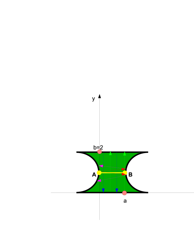
Figure 12: The anti-Bunimovich billiards with the bouncing mode skeleton deprived of the scar generating bundles associated with the horizontal periodic orbit

whole billiards interfere everywhere chaotically, i.e. typically as in the cases without scars and satisfying Berry’s conjecture [26]. Some order in such interfering can be organized as we can try to argue by the presence of periodic orbits supported by the focusing properties of the billiards boundary in vicinities of top points, i.e. the points where periodic orbits touch the billiards boundary.

The last condition, i.e. the focusing properties of the billiards boundary at the top points seems to be essential for the scar phenomenon to appear. One can be convinced of its necessity by considering an ”anti-Bunimovich” stadium, i.e. the stadium which semicircular parts instead of being concave are convex for the billiards, see Fig.12. The horizontal periodic orbit still exists but a skeleton with the properties discussed earlier certainly does not, i.e. the bundles containing this periodic orbit can be only scattered so that the only rays of these bundles which come back close to the periodic orbit is the orbit itself. All the remaining rays even close to the periodic orbits are scattered away passing by the virtual focus points of the convex semicircles.

The results of Barnett’s calculations demonstrated by Sarnak [24, 25] seem also to confirm this conclusion.

Let us note however that the above analysis is not sufficient to estimate the energy corresponding to the mode described above even its lowest JWKB approximation investigating only a vicinity of the horizontal periodic orbit . This is because after every reflection the corresponding half of the horizontal periodic orbit belongs to a new bundle, i.e. this orbit is in fact not closed on the skeleton considered and moreover it does not end in the initial bundle (this is why it is not periodic inside the skeleton). Because of that this classically periodic orbit cannot be used to write on it ”the last quantization condition” of the form (49). In fact such a single periodic orbit possibility of determining the energy would question the role of the eigenfunction boundary conditions in forming its corresponding eigenvalue.

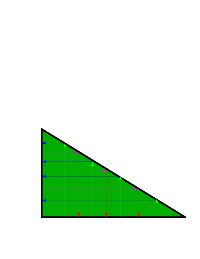
Figure 13: The example of the four bundles skeleton in the right angle triangular billiards on which none semiclassical eigenfunction can be defined

9 Summary and conclusions

We have shown in this paper that it is possible to formulate the semiclassical description of the quantum billiards eigenvalue problems in the semiclassical wave function language. We have used in principle the approach of Maslov and Fedoriuk [6] modifying it however by the way of moving through caustics. The corresponding procedure has been described in App.B. where the idea of continuing semiclassical wave functions by coustic singularities on the complex $t$-plane was developed. It was shown there a close relation between a signature of a SWF and a path along which the SWF has to avoid a caustic singularity on the $t$-plane.

We have also modified the Maslov and Fedoriuk procedure by constructing respective Lagrange manifolds not as smooth, deprived of boundaries tori-like surfaces but rather in the form of skeletons. The skeleton idea has appeared to be sufficiently flexible to gather quantum systems at least in principle uniformly independently of the kind of their semiclassiclal limits, i.e. whether these limits are integrable or chaotic. Nevertheless in the last cases constructions of the corresponding skeletons seem to be rather difficult except these obvious chaotic billiards boundary configurations which have been considered in this paper.

It is worth to stress also at this summary that the forms of skeletons as a set of ray bundles satisfying the geometrical optics law of the mirror-like reflection from the billiards boundary was not a matter of a free choice but a necessity of satisfying the boundary conditions by the SWF’s as it was shown in App.A.

No less important was establishing that in the semiclassical calculations the zeroth order terms of SWF’s are classical integrals of motion. This has allowed us to close the corresponding calculations.

Using known examples of the classically integrable billiards such as the circular and rectangular ones and the broken rectangular billiards as some variants of the rectangular ones we have demonstrated the effectiveness of the skeleton method in the quantization of the systems mentioned. In particular the semiclassical calculations of energy levels performed in sec.5 have developed a new algorithm of finding these levels to any order in Planck constant for the case of the circular billiards (i.e. the cylindrical infinite well).

Applications of the method to other classically integrable billiards systems also in higher than two dimensions are in preparations.

We have shown also how the skeleton method allows us to describe almost trivially the bouncing ball modes in the Bunimovich billiards and similar ones.

We have also discussed a possible explanation of the scar phenomena by the skeleton idea showing a close relation of these phenomenta to focusing properties of billiards boundary in vicinity of the top points of the periodic orbits carrying scars. A lack of focussing properties by the billiards boundary in vicinity of the top points should exclude the existence of scars around the corresponding periodic orbits.

On the other hand it should be stressed that constructing a desired skeleton does not guarantee a construction on it a SWF satisfying desired necessary boundary and other conditions. A simple example of such a situation is a rectangular triangel billiards shown on Fig.13. There is a skeleton collected of four bundles as shown in the figure. It is clear however that none SWF vanishing on the boundary of the billiards can be built on this skeleton.

Appendix A

In this appendix we are going to show, that the geometrical optics rule of reflections of rays off the billiards boundary is a consequence of demands of vanishing on the boundary of the linear combination (35) accompanied by the conditions (36) and (37). Namely consider the following superposition of SWF’s:

$$\Psi_{k}^{as}(x,y;u,l;\lambda)=\Psi_{k,1}^{\sigma_{1}}(d_{1},s_{1};u,l;\lambda)+\Psi_{k,2}^{\sigma_{2}}(d_{2},s_{2};u,l;\lambda)=$$

$$J_{k,1}^{-\frac{1}{2}}(d_{1},s_{1};u,l)e^{i\sigma_{1}k\left(d_{1}+\int_{0}^{s_{1}}\cos\alpha_{k,1}(s^{\prime};u,l)ds^{\prime}\right)}\chi_{k,1}^{\sigma_{1}}(d_{1},s_{1};u,l;\lambda)+$$

$$J_{k,2}^{-\frac{1}{2}}(d_{2},s_{2};u,l)e^{i\sigma_{2}k\left(d_{2}+\int_{0}^{s_{2}}\cos\alpha_{k,2}(s^{\prime};u,l)ds^{\prime}\right)}\chi_{k,2}^{\sigma_{2}}(d_{2},s_{2};u,l;\lambda)$$ (132)

with

$${\bf r}\equiv[x,y]={\bf r}_{k,1}(d_{1},s_{1};u,l)={\bf r}_{0}(s_{1})+{\bf d}_{1}(s_{1};u,l)=$$

$${\bf r}_{k,2}(d_{2},s_{2};u,l)={\bf r}_{0}(s_{2})+{\bf d}_{2}(s_{2};u,l)$$

$${\bf r}_{k,1}(d,s;u,l)\in B_{k}(u,l),\;\;\;\;\;{\bf r}_{k,2}(d,s;u,l)\in B_{k}^{\prime}(u,l),\;\;\;\;B_{k}(u,l)\neq B_{k}^{\prime}(u,l)$$ (133)

i.e. the SWF’s $\Psi_{k,1}^{\sigma_{1}}(d_{1},s_{1};u,l;\lambda)$ and $\Psi_{k,2}^{\sigma_{2}}(d_{2},s_{2};u,l;\lambda)$ are defined respectively on the bundles $B_{k}(u,l)$ and $B_{k}^{\prime}(u,l)$ with $D_{k}(u,l)\cap D_{k}^{\prime}(u,l)\neq\oslash$ interfering in the crossing point $[x,y]$ of two rays ${\bf r}_{k,1}(d_{1},s_{1};u,l)$ and ${\bf r}_{k,2}(d_{2},s_{2};u,l)$ belonging to the respective bundles.

Therefore the condition for $\Psi_{k}^{as}(x,y,\lambda)$ to vanish on $A_{k}(u,l)$ is:

$$J_{k,1}^{-\frac{1}{2}}(0,s)e^{ik\sigma_{1}\int_{0}^{s}\cos\alpha_{k,1}(s^{\prime};u,l)ds^{\prime}}\chi_{k,1}^{\sigma_{1}}(s;u,l;\lambda)+$$

$$J_{k,2}^{-\frac{1}{2}}(0,s)e^{ik\sigma_{2}\int_{0}^{s}\cos\alpha_{k,2}(s^{\prime};u,l)ds^{\prime}}\chi_{k,2}^{\sigma_{2}}(s;u,l;\lambda)=0$$

$${\bf r}_{0}(s)\in A_{k}(u,l)$$ (134)

Because of the $k$-dependence the last relation can be satisfied if and only if:

$$\sigma_{1}\int_{0}^{s}\cos\alpha_{k,1}(s^{\prime};u,l)ds^{\prime}=\sigma_{2}\int_{0}^{s}\cos\alpha_{k,2}(s^{\prime};u,l)ds^{\prime},\;\;\;\;\;\;{\bf r}_{0}(s)\in A_{k}(u,l)$$ (135)

It is easy to see however that there are only two solutions of the last condition:

$$\alpha_{k,1}(s;u,l)\equiv\alpha_{k,2}(s;u,l)\;\;\;\;\;\;\;\;for\;\;\;\;\;\;\;\;\sigma_{1}=\sigma_{2}$$

$$\alpha_{k,1}(s;u,l)\equiv\pi-\alpha_{k,2}(s;u,l)\;\;\;\;\;\;\;\;for\;\;\;\;\;\;\;\;\sigma_{1}=-\sigma_{2}$$

$${\bf r}_{0}(s)\in A_{k}(u,l)$$ (136)

The first solutions are however uninteresting identifying the bundles in a given segment and consequently leading to the solutions vanishing identically on $A_{k}(u,l)$.

Putting $\alpha_{k,1}(s;u,l)\equiv\alpha(s;u,l)$ and $\sigma_{1}=-\sigma$ we get from the second solution and from (134):

$$\chi_{k,2}^{-\sigma}(s;u,l;\lambda)=-\chi_{k,1}^{\sigma}(s;u,l;\lambda)\equiv\chi_{k}(s;u,l;\lambda)$$

$${\bf r}_{0}(s)\in A_{k}(u,l)$$ (137)

so that the combination (35) becomes:

$$\Psi_{k}^{as}(x,y;u,l;\lambda)=\Psi_{k,1}^{\sigma}(d_{1},s_{1};u,l;\lambda)-\Psi_{k,2}^{-\sigma}(d_{2},s_{2};u,l;\lambda)=$$

$$J_{k,1}^{-\frac{1}{2}}(d_{1},s_{1};u,l)e^{i\sigma k\left(d_{1}+\int_{0}^{s_{1}}\cos\alpha(s^{\prime};u,l)ds^{\prime}\right)}\chi_{k,1}^{\sigma}(d_{1},s_{1};u,l;\lambda)-$$

$$J_{k,2}^{-\frac{1}{2}}(d_{2},s_{2};u,l)e^{-i\sigma k\left(d_{2}+\int_{0}^{s_{2}}\cos\alpha(s^{\prime};u,l)ds^{\prime}\right)}\chi_{k,2}^{-\sigma}(d_{2},s_{2};u,l;\lambda)$$

$${\bf r}_{0}(s)\in A_{k}(u,l)$$ (138)

where $\chi_{k}{\sigma}(d,s;u,l;\lambda),\;\sigma=\pm,$ are given by (31) with $\chi_{k}^{\sigma}(0,s;u,l;\lambda)\equiv\chi_{k}(s;u,l;\lambda)$.

The last result shows that $\Psi_{k}^{as}(x,y;u,l;\lambda)$ vanishing on $A_{k}(u,l)$ has to be represented semiclassically by a combination of at least two SWF’s of opposite signatures and such that if $\Psi_{k,1}^{\sigma}(d,s;u,l;\lambda)$ is defined on the bundle $B_{k}(u,l)$ then the second SWF $\Psi_{k,2}^{-\sigma}(d,s;u,l;\lambda)$ has to be defined on the bundle $B_{k}^{A}(u,l)$.

Appendix B

In this appendix we explore the well known properties of the circular billiards to establish the way of avoiding the singular caustic points on the $t$-plane as well as to confirm the way given by (38) by which two SWF’s have been matched.

The circular billiards is of course the well known case of the two dimensional infinitely deep cylindrical potential well which energy spectrum is easily obtained by solving the stationary Schrödinger equation (SSE) for this case by the variable separation method performed in the cylindrical coordinates. In the latter coordinates the radial part of the SSE is the following:

$$\Psi^{\prime\prime}(r)+\frac{1}{r}\Psi^{\prime}(r)+\lambda^{2}\left(E-\frac{m^{2}}{\lambda^{2}r^{2}}\right)\Psi(r)=0$$ (139)

where the separation constant $m=0,\pm 1,...$, is the angular momentum quantum number, $\lambda=\hbar^{-1}$ and we have put $2M=1$ where $M$ is the billiard ball mass.

After the substitution $\Psi(r)=\frac{\psi(r)}{r^{\frac{1}{2}}}$ we get:

$$\psi^{\prime\prime}(r)+\lambda^{2}\left(E-\frac{m^{2}-\frac{1}{4}}{\lambda^{2}r^{2}}\right)\psi(r)=0$$ (140)

Assuming the unit radius of the billiards we get the solutions for (139) in the following forms [27]:

$${\tilde{\psi}}_{\pm}(r)=q^{-\frac{1}{4}}e^{\pm i\lambda\int_{1}^{r}q^{\frac{1}{2}}dr^{\prime}}{\tilde{\chi}}_{\pm}(r),\;\;\;\;r_{+}<r\leq 1$$

$$q=p_{r}^{2}=E-\frac{m^{2}}{\lambda^{2}r^{2}}=\frac{E}{r^{2}}(r-r_{+})(r-r_{-}),\;\;\;\;r_{\pm}=\pm\frac{|m|}{\lambda\sqrt{E}},\;\;\;m\neq 0$$ (141)

which correspond to the fundamental solutions ${\tilde{\psi}}_{+}(r)$ and ${\tilde{\psi}}_{-}(r)$ defined in the respective sectors $1$ i ${\bar{1}}$ of the Stokes graph of Fig.13 with ${\tilde{\chi}}_{\pm}(r)$ normed at the corresponding sector infinities by ${\tilde{\chi}}_{+}(\infty_{1})={\tilde{\chi}}_{-}(\infty_{\bar{1}})=1$. The $r$-plane on this figure has a cut from $r_{+}$ to $r_{-}$ on which $q^{\frac{1}{2}}$ changes its sign, while $q^{-\frac{1}{4}}$ gets the factor $\pm i$ depending on the cut crossing directions ($+i$ for crossing it upwards, $-i$ - for downwards).

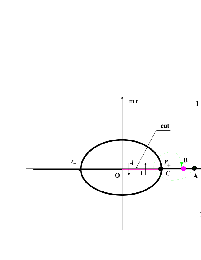
Figure 14: The Stokes graph for the cylindrical billiards

The Stokes graphs formalism corresponding to (141) easily provides us with the energy spectrum of the billiards. For this we take the wave function ${\tilde{\psi}}(r)$ corresponding to this case as a linear combination

$${\tilde{\psi}}(r)={\tilde{\psi}}_{+}(r)+c{\tilde{\psi}}_{-}(r)$$ (142)

given on the segment $AC$ where $c$ is defined by the condition ${\tilde{\psi}}(1)=0$.

It is easy to see that then:

$$c=-\frac{{\tilde{\chi}}_{+}(1)}{{\tilde{\chi}}_{-}(1)}$$ (143)

Next the combination (142) has to be continued to the segment $OC$ vanishing on it when $r\to 0$. This means however that up to a constant it should be identified with the fundamental solution ${\tilde{\psi}}_{0}(r)=q^{-\frac{1}{4}}e^{-i\lambda\int_{r_{+}}^{r}q^{\frac{1}{2}}dr^{\prime}}{\tilde{\chi}}_{0}(r)$, taken for example in this form above the cut $OC$ attached to the sector 0 on Fig.13, i.e. for $r+i\epsilon,\;0<r<r_{+}$.

According to the well known rules the latter can be expressed as the following linear combination of ${\tilde{\psi}}_{\pm}(r)$ [27]:

$${\tilde{\psi}}_{0}(r)=-i{\tilde{\chi}}_{0\to{\bar{1}}}e^{i\lambda\int_{r_{+}}^{1}q^{\frac{1}{2}}dr^{\prime}}{\tilde{\psi}}_{+}(r)+{\tilde{\chi}}_{0\to 1}e^{-i\lambda\int_{r_{+}}^{1}q^{\frac{1}{2}}dr^{\prime}}{\tilde{\psi}}_{-}(r)$$

$$0<r<r_{+}$$ (144)

where ${\tilde{\chi}}_{0\to j}=\lim_{r\to\infty_{j}}{\tilde{\chi}}_{0}(r)$ with $\infty_{j}$ being the infinity point in the sector $j,\;j=1,{\bar{1}}$.

It then follows from (144) that:

$${\tilde{\psi}}(r)=\frac{i}{\chi_{0\to{\bar{1}}}}e^{-i\lambda\int_{r_{+}}^{1}q^{\frac{1}{2}}dr^{\prime}}{\tilde{\psi}}_{0}(r)$$ (145)

and

$$c=i\frac{{\tilde{\chi}}_{0\to 1}}{{\tilde{\chi}}_{0\to{\bar{1}}}}e^{-2i\lambda\int_{r_{+}}^{1}q^{\frac{1}{2}}dr^{\prime}}$$ (146)

The equations (143) and (146) together are just the quantization conditions for the energy with the spectrum of the latter being degenerate with respect to the sign of $m$.

To make further a correspondence with sec.5 we shall use rather the solutions $\psi_{\pm}(r)\equiv{\tilde{\chi}}_{\mp}(1){\tilde{\psi}}_{\pm}(r)$, $\chi_{\pm}(r)\equiv{\tilde{\chi}}_{\mp}(1){\tilde{\chi}}_{\pm}(r)$ and $\psi(r)\equiv{\tilde{\chi}}_{-}(1){\tilde{\psi}}(r)$ in the remaining considerations. Therefore instead of (142) we get simply:

$$\psi(r)=\psi_{+}(r)-\psi_{-}(r)$$ (147)

so that and instead of (146) we have:

$$1=-i\frac{\chi_{1\to 0}}{\chi_{{\bar{1}}\to 0}}e^{-2i\lambda\int_{r_{+}}^{1}q^{\frac{1}{2}}dr^{\prime}}$$ (148)

where $\chi_{1\to 0}={\tilde{\chi}}_{-}(1){\tilde{\chi}}_{1\to 0}$ and $\chi_{{\bar{1}}\to 0}={\tilde{\chi}}_{+}(1){\tilde{\chi}}_{{\bar{1}}\to 0}$ and where we have taken into account that $\chi_{0\to j}=\chi_{j\to 0},\;j=1,{\bar{1}}$.

The results (143)-(148) obtained above are exact.

Consider now the semiclassical limits of (143)-(148), i.e. when $\lambda\to+\infty$. It should be stressed that the fundamental solution formalism allows us to do such a passage and in every of the above formula this limit is well defined. In particular all exponentially small contributions have to be neglected. In this way if $r$ is in sector $0$ such an exponentially small is the solution ${\tilde{\psi}}_{0}(r)$ so that taking the semiclassical limit in (144) we get:

$$0=-i\chi_{{\bar{1}}\to 0}^{as}e^{+i\lambda\int_{r_{+}}^{1}q_{as}^{\frac{1}{2}}dr^{\prime}}\psi_{+}^{as}(r)+\chi_{1\to 0}^{as}e^{-i\lambda\int_{r_{+}}^{1}q_{as}^{\frac{1}{2}}dr^{\prime}}\psi_{-}^{as}(r),\;\;\;\;\;\;\;0<r\leq r_{+}$$

$$\psi_{\pm}^{as}(r)=q_{as}^{-\frac{1}{4}}e^{\pm i\lambda\int_{1}^{r}q_{as}^{\frac{1}{2}}dr^{\prime}}\chi_{\pm}^{as}(r)$$ (149)

where $"as"$ denotes the semiclassical forms of the relevant quantities and in particular $\chi_{\pm}^{as}(r),\;\chi_{{\bar{1}}\to 0}^{as}(=\chi_{0\to 1}^{as})$ and the asymptotic form of $\chi_{1\to 0}^{as}(=\chi_{0\to{\bar{1}}}^{as})$ can be found in any of the references [27] while $q_{as}=E-\frac{m^{2}}{\lambda^{2}r^{2}}$ with $E=E_{0}+\frac{1}{\lambda^{2}}E_{1}+...$.

In fact the linear relation (149) is equivalent to the following identity valid in the semiclassical limit:

$$\chi_{+}^{as}(r)\chi_{{\bar{1}}\to 0}^{as}=\chi_{1\to 0}^{as}\chi_{-}^{as}(r),\;\;\;\;\;\;\;0<r\leq r_{+}$$ (150)

if the point $r,\;r\in OC$, is approached continuing $\chi_{+}^{as}(r)$ anticlockwise and $\chi_{-}^{as}(r)$ - clockwise around the point $C$ of Fig.13.

Taking also the semiclassical limit of the exact quantization condition (148) we get:

$$1=-i\frac{\chi_{1\to 0}^{as}}{\chi_{{\bar{1}}\to 0}^{as}}e^{-2i\lambda\int_{r_{+}}^{1}q^{\frac{1}{2}}dr^{\prime}}$$ (151)

From both (149) and (151) it follows that:

$$\psi_{+}^{as}(r)=\psi_{-}^{as}(r),\;\;\;\;\;\;\;0<r\leq r_{+}$$ (152)

Conversely if (152) is valid then from the identity (149) we get the semiclassical form (151) of the quantization condition.

Therefore both the conditions (148) and (152) are equivalent to each other as the semiclassical quantization conditions in the case considered.

We conclude therefore that the equation (152) substitutes the quantization condition (151) in the semiclassical limit, i.e. in the quantized semiclassical limit both $\psi_{+}^{as}(r)$ and $\psi_{-}^{as}(r)$ has to coincide in the sector 0. But this coincidence can be analytically continued to any (non singular) point of the $r$-plane. In particular it can be continued back to the classically allowed segment $AC$. These can be done in two ways, by avoiding the singular point $C$ clockwise or anticlockwise.

Before making the respective continuations let us note that the relation (144) cannot be continued to the segment $AC$ of the Stokes graph of Fig.13 not loosing its connection with its asymptotic form (149) while this asymptotic form itself can loosing however its connection to the original equation (144). This new form of an equation substituting the original one (144) can be obtained by the Borel resummation procedure.

Let us start therefore with the relation (149) and (152) to continue them to $AC$ around the point $C$ clockwise. We get:

$$0=-i\chi_{{\bar{1}}\to 0}^{as}e^{+i\lambda\int_{r_{+}}^{1}q_{as}^{\frac{1}{2}}dr^{\prime}}\psi_{+}^{as}(r)+\chi_{1\to 0}^{as}e^{-i\lambda\int_{r_{+}}^{1}q_{as}^{\frac{1}{2}}dr^{\prime}}\psi_{-}^{as,cont}(r),\;\;\;\;\;\;\;0<r\leq r_{+}$$

(153)

and

$$\psi_{+}^{as}(r)=\psi_{-}^{as,cont}(r),\;\;\;\;\;\;r_{+}<r\leq 1$$ (154)

where $\psi_{-}^{as,cont}(r)$ denotes $\psi_{-}^{as}(r)$ continued analytically clockwise around the point $C$ from the segment $AC$ to the same segment.

If we choose the opposite path of continuation, i.e. anticlockwise one, then continuing the relation (152) we get:

$$0=-i\chi_{{\bar{1}}\to 0}^{as}e^{+i\lambda\int_{r_{+}}^{1}q_{as}^{\frac{1}{2}}dr^{\prime}}\psi_{+}^{as,cont}(r)+\chi_{1\to 0}^{as}e^{-i\lambda\int_{r_{+}}^{1}q_{as}^{\frac{1}{2}}dr^{\prime}}\psi_{-}^{as,cont}(r),\;\;\;\;\;\;\;0<r\leq r_{+}$$

(155)

and

$$\psi_{-}^{as}(r)=\psi_{+}^{as,cont}(r),\;\;\;\;\;\;r_{+}<r\leq 1$$ (156)

where $\psi_{+}^{as,cont}(r)$ denotes $\psi_{+}^{as}(r)$ continued analytically anticlockwise around the point $C$ from the segment $AC$ to the same segment.

However, contrary to $OC$ the segment $AC$ lies now totally in the common part of the domains of Borel summability of $\psi_{\pm}(r)$ so that we have:

$$\left(\psi_{\pm}^{as}(r)\right)^{BS}=\psi_{\pm}(r),\;\;\;\;\;\;r_{+}<r\leq 1$$ (157)

where the superscript $BS$ means the Borel resummation of the relevant quantity.

But according to (154) i (156) we have instead:

$$\left(\psi_{\pm}^{as,cont}(r)\right)^{BS}=\psi_{\mp}(r)$$

$$r_{+}<r\leq 1$$ (158)

while by the Borel summing (153) and (155) we obtain respectively:

$$\left(\psi_{-}^{as,cont}(r)\right)^{BS}=i\frac{\chi_{{\bar{1}}\to 0}}{\chi_{1\to 0}}e^{+2i\lambda\int_{r_{+}}^{1}q^{\frac{1}{2}}dr^{\prime}}\psi_{+}(r)$$

$$\left(\psi_{+}^{as,cont}(r)\right)^{BS}=-i\frac{\chi_{1\to 0}}{\chi_{{\bar{1}}\to 0}}e^{-2i\lambda\int_{r_{+}}^{1}q^{\frac{1}{2}}dr^{\prime}}\psi_{-}(r)$$

$$0<r\leq r_{+}$$ (159)

If we now apply the Borel summed quantization conditions (158) to the respective equations in (159) we immediately recover the exact quantization condition (148).

Let us summarize the above results.

• In the semiclassical limit the quantization condition for the circular billiards is the appropriate coincidence of the asymptotic expansions of two fundamental solutions in the classically unallowed region (the segment $OC$). This coincidence is given by (152).

• In the classically allowed region the semiclassical quantization condition can be obtained by continuing appropriately (clockwise or anticlockwise) one of the semiclassical solutions $\psi_{\pm}^{as}(r)$ from the segment $AC$ and back to it around the turning point $C$ and next by identifying the continued solution with the second one. The respective identifications are given by (154) and (156).

• The semiclassical quantization conditions formulated in the classically allowed as well as in unallowed regions can be Borel summable leading us to the exact ones;

• The fundamental semiclassical solutions continued to the classically allowed region (the segment $AC$) by the unallowed one (the segment $OC$) still represent semiclassical expansions of some fundamental solutions which by Borel resummation can be identified appropriately (see the formulae (159)).

• The semiclassical quantization condition formulated by (154) and (156) in the classically allowed region (the segment $AC$) can be Borel summable providing us with the proper exact quantization conditions.

B.1 The fundamental solutions semiclassical analysis rewritten on the classical trajectories

Let us now rewrite the above results in the formalism of the SWF’s defined on the classical trajectories developed in sec.5.

To this goal let us assume the semiclassical expansion (12) for the energy $E$ so that the classical momentum $p=\sqrt{2E_{0}}$, and associate with the solution (142) two bundle skeletons ${\bf B}$ and ${\bf B}_{A}$.

Both the skeletons consist of single ray bundles only. The skeleton ${\bf B}$ consists of the ray bundle $B(0,2\pi)$ the rays of which run with the definite positive angular momentum $m,\;m=1,2,...,$ and with momenta ${\bf p}$ shown in Fig.2 while the angular momentum of the skeleton ${\bf B}^{A}$ is equal to $-m$ and rays of its unique bundle $B^{A}(0,2\pi)$ have momenta ${\bf p}^{A}$ on Fig.2. For both the momenta we have $|{\bf p}|=|{\bf p}^{A}|=p$.

Any point of the ring $(r,\Phi),\;r_{+}<r\leq 1,\;0\leq\Phi<2\pi$, is crossed by two rays coming from different bundles starting from the points $s_{1}$ and $s_{2}$ of the billiard boundary and having the respective angular momenta equal to $p\cos\alpha=m/\lambda$ and $p\cos(\pi-\alpha)=-m/\lambda$ with $\cos\alpha=r_{+}$ (see Fig.2) while their corresponding radial momenta are the same and equal to $p_{r}={\dot{r}}=\frac{p^{2}(t-t_{c})}{r(t)}=-\sqrt{E_{0}-\frac{p^{2}\cos^{2}\alpha}{r^{2}}}=-\sqrt{E_{0}-\frac{m^{2}}{\lambda^{2}r^{2}}}\equiv-q_{0}^{\frac{1}{2}}$ being negative ($t<t_{c},\;t_{c}=\sin\alpha/p$).

Starting at the moment $t=0$ from the boundary these rays meet each other at the point $(r,\Phi)$ in the moment $t$.

Each of the bundles defines a transformation of coordinate $(r,\Phi)\to(d,s_{i}),\;i=1,2,$ by $r=r(d)=\sqrt{\cos^{2}\alpha+(\sin\alpha-d)^{2}},\;d=pt$ and $\Phi=s_{1}+\alpha-\gamma=s_{2}-\alpha+\gamma<s_{1}+\alpha$ correspondingly to the bundle, see Fig.2.

The total original solution

$$\Psi(r,\Phi)=\frac{\psi(r)}{r^{\frac{1}{2}}}e^{im\Phi}$$ (160)

corresponding to (147) can be now rewritten by the new coordinates noticing that $\int_{1}^{r}q_{0}^{\frac{1}{2}}dr^{\prime}=-\int_{1}^{r}p_{r}dr^{\prime}=-\int_{0}^{t}p_{r}^{2}dt^{\prime}=-\int_{0}^{t}p^{2}dt^{\prime}+\int_{0}^{t}\frac{p_{\Phi}^{2}}{r^{2}}dt^{\prime}=-p^{2}t+p^{2}\cos^{2}\alpha\int_{0}^{t}\frac{dt^{\prime}}{r^{2}(t^{\prime})}$ and that

$$\int_{0}^{t}\frac{dt^{\prime}}{r^{2}(t^{\prime})}=\left.\frac{1}{\cos\alpha}\arctan\frac{p(t^{\prime}-t_{c})}{\cos\alpha}\right|_{0}^{t}=\frac{1}{\cos\alpha}(\alpha-\gamma)$$ (161)

for $t<t_{c}$ so that:

$$\psi_{\pm}(r(t),\lambda)=q_{0}^{-\frac{1}{4}}e^{\mp i\lambda p^{2}t\pm i|m|(\alpha-\gamma)}\chi_{\pm}(t,\lambda)$$

$$\chi_{\pm}(t,\lambda)=\left(\frac{q}{q_{0}}\right)^{-\frac{1}{4}}e^{\mp i\lambda\int_{0}^{t}\left(q^{\frac{1}{2}}-q_{0}^{\frac{1}{2}}\right)q_{0}^{\frac{1}{2}}dt^{\prime}}{\chi}_{\pm}(r(t),\lambda)=$$

$$\left(\frac{q}{q_{0}}\right)^{-\frac{1}{4}}\exp\left[\mp i\sum_{n\geq 0}E_{n+1}\lambda^{-n-1}\int_{0}^{d}\frac{1}{1+\left(\frac{q}{q_{0}}\right)^{\frac{1}{2}}}dt^{\prime}\right]{\chi}_{\pm}(r(t),\lambda)$$

$$\frac{q}{q_{0}}=1+\frac{\sum_{n\geq 1}E_{n}\lambda^{-n-1}}{q_{0}}$$ (162)

and then we get:

$$\Psi(r,\Phi)=\frac{\psi_{+}(r(t))-\psi_{-}(r(t))}{r^{\frac{1}{2}}(t)}e^{im\Phi}=$$

$$(r^{2}q_{0})^{-\frac{1}{4}}e^{-i\lambda p^{2}t+i|m|(\alpha-\gamma)+im\Phi}\chi_{+}(t,\lambda)-(r^{2}q_{0})^{-\frac{1}{4}}e^{+i\lambda p^{2}t-i|m|(\alpha-\gamma)+im\Phi}\chi_{-}(t,\lambda)$$ (163)

where $(r^{2}q_{0})^{-\frac{1}{4}}\equiv(r^{2}(t)q_{0}(t))^{-\frac{1}{4}}=(E_{0}(r^{2}(t)-r_{+}^{2}))^{-\frac{1}{4}}=p^{-1}|t-t_{c}|^{-\frac{1}{2}}$.

From (163) we get further:

$$\Psi(r,\Phi)=\left\{\begin{array}[]{lr}(r^{2}q_{0})^{-\frac{1}{4}}e^{-i\lambda p^{2}t+ims_{2}}\chi_{+}(t,\lambda)-(r^{2}q_{0})^{-\frac{1}{4}}e^{i\lambda p^{2}t+ims_{1}}\chi_{-}(t,\lambda),&m>0\\ (r^{2}q_{0})^{-\frac{1}{4}}e^{-i\lambda p^{2}t+ims_{1}}\chi_{+}(t,\lambda)-(r^{2}q_{0})^{-\frac{1}{4}}e^{i\lambda p^{2}t+ims_{2}}\chi_{-}(t,\lambda),&m<0\end{array}\right.=$$ (166)

$$\left\{\begin{array}[]{lr}p^{-1}|t-t_{c}|^{-\frac{1}{2}}e^{-i\lambda p^{2}t-i\lambda ps_{2}\cos(\pi-\alpha)}\chi_{+}(t,\lambda)-&\\ p^{-1}|t-t_{c}|^{-\frac{1}{2}}e^{i\lambda p^{2}t+i\lambda ps_{1}\cos\alpha}\chi_{-}(t,\lambda),&m>0\\ p^{-1}|t-t_{c}|^{-\frac{1}{2}}e^{-i\lambda p^{2}t-i\lambda ps_{1}\cos\alpha}\chi_{+}(t,\lambda)-&\\ p^{-1}|t-t_{c}|^{-\frac{1}{2}}e^{i\lambda p^{2}t+i\lambda ps_{2}\cos(\pi-\alpha)}\chi_{-}(t,\lambda),&m<0\end{array}\right.\;\;\;\;\;\;\;=$$ (171)

$$\left\{\begin{array}[]{lr}i\Psi^{-}(t,s_{2})-i\Psi^{+}(t,s_{1}),&m>0\\ i\Psi^{-}(t,s_{1})-i\Psi^{+}(t,s_{2}),&m<0\end{array}\right.$$ (174)

where $\Psi^{\pm}(t,s_{j}),\;j=1,2$, have the form (26) but are exact. We have also assumed that $(t-t_{c})^{-\frac{1}{2}}=-i|t-t_{c}|^{-\frac{1}{2}}$ for $t<t_{c}$ (see below).

The last result shows that, depending on $m$, the bundles on which the fundamental solutions $\psi_{\pm}(r)$ are defined are chosen by the latter accordingly to their signatures.

Let us now consider the analytical continuation of the semiclassical limit $\Psi^{as}(r,\Phi)$ of the solution $\Psi(r,\Phi)$ from the point $A$ to its point $B$ as it is defined by the rule (154) or back, i.e. from $B$ to $A$ correspondingly to the rule (156), see Fig.2.

Since $t=t_{c}-\frac{1}{p}\sqrt{(r-r_{+})(r+r_{+})}$ then, if $r$ rounds the turning point $C$ by $2\pi$ clockwise starting from the segment $AC$ (see Fig.13), $t$ rounds $t_{c}$ on the $t$-plane also clockwise by $\pi$. But $t$ rounds $t_{c}$ by $\pi$ anticlockwise if $r$ does the previous motion in the opposite direction. In both the cases we are found at the point $B$ with $t>t_{c}$. However in the first case $(t-t_{c})^{-\frac{1}{2}}=|t-t_{c}|^{-\frac{1}{2}}$ while in the second $(t-t_{c})^{-\frac{1}{2}}=-|t-t_{c}|^{-\frac{1}{2}}$.

$\Psi^{as}(r,\Phi)$ continued clockwise on the $r$-Riemann surface is given by:

$$\Psi_{clock}^{as}(r,\Phi)=\frac{\psi_{+}^{as}(r)-\psi_{-}^{as,cont}(r)}{r^{\frac{1}{2}}}e^{im\Phi}=\frac{1}{r^{\frac{1}{2}}}\left(1-ie^{-2i\lambda\int_{1}^{r_{+}}q^{\frac{1}{2}}dr^{\prime}}\frac{\chi_{{\bar{1}}\to 0}^{as}}{\chi_{1\to 0}^{as}}\right)\psi_{+}^{as}(r)e^{im\Phi}$$

$$r_{+}<r<1$$ (175)

where $\psi_{-}^{as,cont}(r)$ has been substituted by its form which follows from (155).

Continued however anticlockwise it is given by:

$$\Psi_{anticlock}^{as}(r,\Phi)=\frac{\psi_{+}^{as,cont}(r)-\psi_{-}^{as}(r)}{r^{\frac{1}{2}}}e^{im\Phi}=\frac{1}{r^{\frac{1}{2}}}\left(1+ie^{+2i\lambda\int_{1}^{r_{+}}q^{\frac{1}{2}}dr^{\prime}}\frac{\chi_{1\to 0}^{as}}{\chi_{{\bar{1}}\to 0}^{as}}\right)\psi_{-}^{as}(r)e^{im\Phi}$$

$$r_{+}<r<1\;\;\;\;\;\;$$ (176)

where $\psi_{+}^{as,cont}(r)$ has been substituted by its form given by (153).

Note that in both the above continuations we have not taken into account the quantization conditions (154) and (156).

However if the energy is to be quantized we have to have:

$$\Psi_{clock}^{as}(r,\Phi)=\Psi_{anticlock}^{as}(r,\Phi)\equiv 0$$ (177)

Performing now in (175) and (176) the calculations similar to the ones above but with the variables $t,\;t>t_{c},$ we get from (174) and (175), see Fig.7:

$$\Psi_{clock}^{as}(r,\Phi)=\left\{\begin{array}[]{lr}-i\Psi^{+,cont}(t,s_{1})+i\Psi^{-}(2t_{c}-t,s_{2}),&m>0\\ -i\Psi^{+,cont}(t,s_{2})+i\Psi^{-}(2t_{c}-t,s_{1})),&m<0\end{array}\right.=$$ (180)

$$\left\{\begin{array}[]{lr}-ip^{-1}|t-t_{c}|^{-\frac{1}{2}}\frac{\chi_{{\bar{1}}\to 0}^{as}}{\chi_{1\to 0}^{as}}e^{i\lambda p^{2}t+i\lambda ps_{1}\cos\alpha}\chi_{+}^{as}(t,\lambda)+&\\ p^{-1}|t-t_{c}|^{-\frac{1}{2}}e^{-i\lambda p^{2}(2t_{c}-t)-i\lambda ps_{2}\cos(\pi-\alpha)}\chi_{+}^{as}(2t_{c}-t,\lambda),&m>0\\ -ip^{-1}|t-t_{c}|^{-\frac{1}{2}}\frac{\chi_{{\bar{1}}\to 0}^{as}}{\chi_{1\to 0}^{as}}e^{i\lambda p^{2}t+i\lambda ps_{2}\cos(\pi-\alpha)}\chi_{+}^{as}(t,\lambda)+&\\ p^{-1}|t-t_{c}|^{-\frac{1}{2}}e^{-i\lambda p^{2}(2t_{c}-t)-i\lambda ps_{1}\cos\alpha}\chi_{+}^{as}(2t_{c}-t,\lambda),&m<0\end{array}\right.$$ (185)

$$2t_{c}>t>t_{c},\;\;\;\;\;s_{2}=s_{1}\pm 2\alpha$$ (186)

where $\Psi^{+,cont}(t,s_{j}),\;t>t_{c}$, are the results of the continuations of $\Psi^{+}(t,s_{j}),\;t<t_{c},\;j=1,2$, by the caustic.

For $\Psi_{anticlock}^{as}(r,\Phi)$ we get instead:

$$\Psi_{anticlock}^{as}(r,\Phi)=\left\{\begin{array}[]{lr}-i\Psi^{+}(2t_{c}-t,s_{1})+i\Psi^{-,cont}(t,s_{2}),&m>0\\ -i\Psi^{+}(2t_{c}-t,s_{2})+i\Psi^{-,cont}(t,s_{1})),&m<0\end{array}\right.=$$ (189)

$$\left\{\begin{array}[]{lr}-p^{-1}|t-t_{c}|^{-\frac{1}{2}}e^{i\lambda p^{2}(2t_{c}-t)+i\lambda ps_{1}\cos\alpha}\chi_{-}^{as}(2t_{c}-t,\lambda)+&\\ -ip^{-1}|t-t_{c}|^{-\frac{1}{2}}\frac{\chi_{1\to 0}^{as}}{\chi_{{\bar{1}}\to 0}^{as}}e^{-i\lambda p^{2}t-i\lambda ps_{2}\cos(\pi-\alpha)}\chi_{-}^{as}(t,\lambda),&m>0\\ -p^{-1}|t-t_{c}|^{-\frac{1}{2}}e^{i\lambda p^{2}(2t_{c}-t)+i\lambda ps_{2}\cos(\pi-\alpha)}\chi_{-}^{as}(2t_{c}-t,\lambda)+&\\ -ip^{-1}|t-t_{c}|^{-\frac{1}{2}}\frac{\chi_{1\to 0}^{as}}{\chi_{{\bar{1}}\to 0}^{as}}e^{-i\lambda p^{2}t-i\lambda ps_{1}\cos\alpha}\chi_{-}^{as}(t,\lambda),&m<0\end{array}\right.$$ (194)

$$2t_{c}>t>t_{c},\;\;\;\;\;s_{2}=s_{1}\pm 2\alpha$$ (195)

where $\Psi^{-,cont}(t,s_{j}),\;t>t_{c}$, are the results of the continuations of $\Psi^{-}(t,s_{j}),\;t<t_{c},\;j=1,2$, by the caustic.

From the above considerations it follows clearly that $\Psi^{+}(t,s)$ continued through the caustic has to avoid the focusing point at $t=t_{c}$ from above in the $t$-plane, moving clockwise while $\Psi^{-}(t,s)$ - from below, moving anticlockwise. By such a continuation $\Psi^{+}(t,s)$ acquires the factor $i$ while $\Psi^{-}(t,s)$ - the factor $-i$.

Let us summarize the above results.

1. The SWF $\Psi^{as}(x,y)$ for the circular billiards originally defined closely to the boundary of the billiards and vanishing on the boundary can be written as the combinations (174) of the two SWF $\Psi^{\pm}(t,s)$ of the opposite signatures having the forms given by (26) and defined on the two skeletons ${\bf B}$ and ${\bf B}^{A}$.

2. It is the SWF $\Psi^{+}(t,s)$ which is defined on the skeleton B which momenta being tangential to the caustic of the bundle give the anticlockwise orientation of the caustic for $m>0$ but on the skeleton ${\bf B}^{A}$ for $m<0$. The SWF $\Psi^{-}(t,s)$ is then defined on the second skeleton in the respective cases.

3. $\Psi^{as}(x,y)$ can be continued across the caustic avoiding the real singular point at $t=t_{c}$ on the $t$-plane from above for $\Psi^{+}(t,s)$ and from below - for $\Psi^{-}(t,s)$ and getting then the forms (186) or (195).

4. If $\Psi^{as}(x,y)$ is to be quantized then $\Psi^{as,cont}(x,y)$ has to vanish identically independently of the way (clockwise or anticlokcwise) it was continued. In such a case we have to have:

   $$\Psi^{\pm,cont}(t,s)=\Psi^{\mp}(2t_{c}-t,s\pm 2\alpha),\;\;\;\;\;t>t_{c}$$ (196)

   leading to for $t=2t_{c}$:

   $$\frac{\chi_{{\bar{1}}\to 0}^{as}(E,\lambda)}{\chi_{1\to 0}^{as}(E,\lambda)}\exp\left[i\sum_{n\geq 0}E_{n+1}\lambda^{-n}\int_{0}^{2t_{c}}\frac{1}{1+\left(\frac{q}{q_{0}}\right)^{\frac{1}{2}}}dt^{\prime}\right]e^{i\lambda p^{2}2t_{c}-2i\lambda\alpha p\cos\alpha+i\frac{1}{2}\pi}=1$$ (197)

   where we have taken into account that $r(2t_{c}-t)=r(t)$.

5. In the limit $\lambda\to\infty$ the condition (197) decays into the following ones:

   $$e^{i\lambda pd(s,\alpha)-2i\lambda\alpha p\cos\alpha+i\frac{1}{2}\pi}=1$$

   $$\frac{\chi_{{\bar{1}}\to 0}^{as}(E,\lambda)}{\chi_{1\to 0}^{as}(E,\lambda)}\exp\left[i\sum_{n\geq 0}E_{n+1}\lambda^{-n}\int_{0}^{2t_{c}}\frac{1}{1+\left(\frac{q}{q_{0}}\right)^{\frac{1}{2}}}dt^{\prime}\right]=1$$

   $$d(s,\alpha)=2pt_{c}=2\sin\alpha$$ (198)

   Of course the condition (197) coincides with (146).

6. The two degenerate SWF’s $\Psi^{as,\pm}(x,y)$ in each point inside the ring $\cos\alpha<r\leq 1$ can be given by:

   $$\Psi^{as,+}(x,y)=-i\Psi^{+}(t,s_{1})+i\Psi^{+,cont}(2t_{c}-t,s_{2}-2\alpha)=$$

   $$i\Psi^{-}(t,s_{2})-i\Psi^{-,cont}(2t_{c}-t,s_{1}+2\alpha),\;\;\;\;\;\;m>0$$ (199)

   $$\Psi^{as,-}(x,y)=-i\Psi^{+}(t,s_{2})+i\Psi^{+,cont}(2t_{c}-t,s_{1}-2\alpha)=$$

   $$-i\Psi^{-,cont}(2t_{c}-t,s_{2}+2\alpha)+i\Psi^{-}(t,s_{1}),\;\;\;\;\;\;m<0$$

   $$t<t_{c}$$ (200)

Appendix C

It is shown in this appendix that $\delta_{k}(u,l)$ from the formula (33) and $\delta(u_{j},l_{j})$ from the formula (39) are $s$-independent. To this end consider Fig.1 on which a mapping $h_{k}(s;u,l)$ of the arc $A_{k}(u,l)$ into an arc $A_{k^{\prime}}(u^{\prime},l^{\prime})$ is defined by the the bundle $B_{k}(u,l)$. According to this mapping we have:

$${\bf r}_{0}(h_{k}(s;u,l))={\bf r}_{0}(s)+{\bf D}(s;u,l)$$

$${\bf r}_{0}(s)\in A_{k}(u,l),\;\;\;\;\;\;{\bf r}_{0}(h_{k}(s;u,l))\in A_{k^{\prime}}(u^{\prime},l^{\prime})$$ (201)

where ${\bf D}(s;u,l)$ is a vector linking the point ${\bf r}_{0}(s)$ with the point ${\bf r}_{0}(h_{k}(s;u,l))$ of the billiards boundary.

Differentiating the equation (201) with respect to $s$ we get:

$$\frac{\partial h_{k}(s;u,l)}{\partial s}\cos\beta(h_{k}(s;u,l))=\cos\beta(s)-D(s;u,l)\frac{\partial\gamma_{k}(s;u,l)}{\partial s}\sin\gamma_{k}(s;u,l)+$$

$$\cos\gamma_{k}(s;u,l)\frac{\partial D(s;u,l)}{\partial s}$$

$$\frac{\partial h_{k}(s;u,l)}{\partial s}\sin\beta(h_{k}(s;u,l))=\sin\beta(s)+D(s;u,l)\frac{\partial\gamma_{k}(s;u,l)}{\partial s}\cos\gamma_{k}(s;u,l)+$$

$$\sin\gamma_{k}(s;u,l)\frac{\partial D(s;u,l)}{\partial s}$$ (202)

where $D(s;u,l)$ is the length of ${\bf D}(s;u,l)$.

Making further the proper linear combinations of the last equations we have finally:

$$\frac{\partial h_{k}(s;u,l)}{\partial s}\cos\alpha_{k^{\prime}}(h_{k}(s;u,l);u^{\prime},l^{\prime})=\cos\alpha_{k}(s;u,l)+\frac{\partial D(s;u,l)}{\partial s}$$

$$-\frac{\partial h_{k}(s;u,l)}{\partial s}\sin\alpha_{k^{\prime}}(h_{k}(s;u,l);u^{\prime},l^{\prime})=\sin\alpha_{k}(s;u,l)-D(s;u,l)\frac{\partial\gamma_{k}(s;u,l)}{\partial s}$$ (203)

where we have taken into account the following relation between the angles involved:

$$\alpha_{k^{\prime}}(h_{k}(s;u,l);u^{\prime},l^{\prime})+\alpha_{k}(s;u,l)=\beta(h_{k}(s;u,l))-\beta(s)+2\pi$$

$$\gamma_{k}(s;u,l)=\beta(s)+\alpha_{k}(s;u,l)$$ (204)

which follows from Fig.1.

The independence of $s$ of $\delta_{k}(u,l)$ and $\delta(u_{j},l_{j})$ follows now easily from the first of the relations (203).

Appendix D

The billiard Laplacean expressed by the variables $d,s$ has the following form:

$$\bigtriangleup(d,s)=\left(\frac{\cos^{2}\alpha}{J^{2}}+1\right)\frac{\partial}{\partial d^{2}}+\frac{1}{J^{2}}\frac{\partial^{2}}{\partial s^{2}}-\frac{2\cos\alpha}{J^{2}}\frac{\partial^{2}}{\partial s\partial d}+$$

$$\left(\frac{\cos\alpha}{J^{3}}\left((\alpha^{\prime}+\gamma^{\prime})\cos\alpha-\frac{\gamma^{\prime\prime}}{\gamma^{\prime}}\sin\alpha\right)+\frac{1}{J^{2}}\left(\frac{\gamma^{\prime\prime}}{\gamma^{\prime}}\cos\alpha+\alpha^{\prime}\sin\alpha\right)-\frac{\gamma^{\prime}}{J}\right)\frac{\partial}{\partial d}-$$

$$\left(\frac{1}{J^{3}}\left((\alpha^{\prime}+\gamma^{\prime})\cos\alpha-\frac{\gamma^{\prime\prime}}{\gamma^{\prime}}\sin\alpha\right)+\frac{\gamma^{\prime\prime}}{\gamma^{\prime}}\frac{1}{J^{2}}\right)\frac{\partial}{\partial s}$$

$$J=\sin\alpha-\gamma^{\prime}d$$ (205)

while for the corresponding operator $J^{\frac{1}{2}}\cdot\bigtriangleup\cdot J^{-\frac{1}{2}}$ we get:

$$J^{\frac{1}{2}}\cdot\bigtriangleup\cdot J^{-\frac{1}{2}}=\frac{3}{4}J^{-2}(\nabla J)^{2}-J^{-1}\nabla J\cdot\nabla-\frac{1}{2}J^{-1}\bigtriangleup J+\bigtriangleup$$

$$(\nabla J)^{2}=\frac{{\gamma^{\prime}}^{2}}{J^{2}}\left(d^{2}-2d\sin\alpha+1\right)+\frac{2\gamma^{\prime}}{J^{3}}(\alpha^{\prime}\cos\alpha-d\gamma^{\prime\prime})\cos\alpha+\frac{1}{J^{2}}(\alpha^{\prime}\cos\alpha-d\gamma^{\prime\prime})^{2}$$

$$\nabla J\cdot\nabla=-\left(\frac{\gamma^{\prime}}{J^{2}}\left(d^{2}-2d\sin\alpha+1\right)+\frac{1}{J^{2}}(\alpha^{\prime}\cos\alpha-d\gamma^{\prime\prime})\cos\alpha\right)\frac{\partial}{\partial d}+$$

$$\left(\frac{1}{J^{2}}(\alpha^{\prime}\cos\alpha-d\gamma^{\prime\prime})+\frac{\gamma^{\prime}\cos\alpha}{J^{2}}\right)\frac{\partial}{\partial s}$$

$$\bigtriangleup J=\frac{1}{J^{2}}\frac{\partial^{2}}{\partial s^{2}}(\sin\alpha-\gamma^{\prime}d)+\frac{2\gamma^{\prime\prime}\cos\alpha}{J^{2}}-$$

$$\frac{\gamma^{\prime}}{J^{3}}\left((\alpha^{\prime}\cos\alpha-d\gamma^{\prime\prime})\cos\alpha-(\beta^{\prime}\sin\alpha-d{\gamma^{\prime}}^{2})(\sin\alpha-\gamma^{\prime}d)\right)-\frac{\gamma^{\prime}\cos\alpha}{J^{3}}(\alpha^{\prime}\cos\alpha-d\gamma^{\prime\prime})$$ (206)

For the circular billiards the corresponding Laplacean takes the forms:

$$\bigtriangleup(d,s)=\frac{1}{J^{2}}\left(d^{2}-2d\sin\alpha+1\right)\frac{\partial^{2}}{\partial d^{2}}+\frac{1}{J^{2}}\frac{\partial^{2}}{\partial s^{2}}-\frac{2\cos\alpha}{J^{2}}\frac{\partial^{2}}{\partial s\partial d}-\frac{1}{J}\frac{\partial}{\partial d}-\frac{\cos\alpha}{J^{3}}\frac{\partial}{\partial s}$$

$$J=\sin\alpha-d$$ (207)

while the corresponding operator $J^{\frac{1}{2}}\cdot\bigtriangleup\cdot J^{-\frac{1}{2}}$ the form:

$$J^{\frac{1}{2}}\cdot\bigtriangleup\cdot J^{-\frac{1}{2}}(d,s)=\frac{3}{4J^{4}}\left(d^{2}-2d\sin\alpha+1\right)+\frac{1}{J^{3}}\left(d^{2}-2d\sin\alpha+1\right)\frac{\partial}{\partial d}-\frac{\cos\alpha}{J^{3}}\frac{\partial}{\partial s}+$$

$$\frac{1}{2J^{2}}+\bigtriangleup(d,s)$$ (208)

For the rectangular billiards the corresponding Laplacean has the following two similar forms depending on the rectangular sides:

$$\bigtriangleup(d,s)=\frac{1}{\sin^{2}\alpha}\left(\frac{\partial^{2}}{\partial d^{2}}+\frac{\partial^{2}}{\partial s^{2}}\right)\mp\frac{2\cos\alpha}{\sin^{2}\alpha}\frac{\partial^{2}}{\partial s\partial d}$$

$$\bigtriangleup(d,s)=\frac{1}{\cos^{2}\alpha}\left(\frac{\partial^{2}}{\partial d^{2}}+\frac{\partial^{2}}{\partial s^{2}}\right)\mp\frac{2\sin\alpha}{\cos^{2}\alpha}\frac{\partial^{2}}{\partial s\partial d}$$ (209)

and of course $J^{\frac{1}{2}}\cdot\bigtriangleup\cdot J^{-\frac{1}{2}}\equiv\bigtriangleup$ for this case of the billiards.

References

- [1] Landau L. D., Lifshitz E. M., Quantum Mechanics. Nonrelativistic Theory (Oxford, New York: Pergamon Press 1965)
- [2] Feynman R.P. and Hibbs A.R., Quantum Mechanics and Path Integrals (New York: McGraw-Hill 1965)
- [3] Schulman L.S., ”Techniques and Applications of Path Integration” (New York: John Wiley 1981)
- [4] Gutzwiller M. C., ”Chaos in Classical and Quantum Mechanics” (New York: Springer 1990)
- [5] Arnold V.I., Mathematical Methods of Classical Mechanics (Berlin: Springer Verlag 1978)
- [6] Maslov V.I. and Fedoriuk M.V., Semi-classical Approximation in Quantum Mechanics (Dordrecht, Boston, London: Reidel 1981)
- [7] Ott E., Chaos in Dynamical Systems (Cambridge MA: Cambridge University Press 1993)
- [8] P. Cvitanović, R. Artuso, R. Mainieri, G. Tanner and G. Vattay, Chaos: Classical and Quantum, ChaosBook.org (Niels Bohr Institute, Copenhagen 2009)
- [9] McDonald S.W. and Kaufman A.N., Phys. Rev. Lett. 42, (1979) 1189
- [10] McDonald S.W., PhD Thesis University of California, Lawrence Berkeley Laboratory, Report no 14837 (1983) (unpublished)
- [11] Bunimovich L.A., Chaos 11 (2001) 802
- [12] B. Dietz, T. Friedrich, M. Miski-Oglu, A. Richter, and F. Schäfer, Phys. Rev. E 75, (2007) 035203
- [13] Alex H. Barnett and Timo Betcke, Chaos 17 (2007) 043125
- [14] Heller E.J., Phys. Rev. Lett. 53, (1984) 1515
- [15] L. Kaplan and E.J. Heller, Phys. Rev. E 59 (1999) 6609 6628
- [16] Heller E.J., Physica Scrypta 2001 (2001) 154
- [17] Sridhar S., Phys. Rev. Lett 67 (1991) 795
- [18] Chinnery P.A. and Humphrey V.F.,Phys. Rev. E, 53 (1996) 272
- [19] Fernando P. Simonotti, Eduardo Vergini, Marcos Saraceno, Quantitative study of scars in the boundary section of the stadium billiard, chao-dyn/9706024v1
- [20] Burq N., Zworski M., SIAM REVIEW 47 (2005) 43
- [21] Burq N., Zworski M., Eigenfunctions for partially rectangular billiards, arXiv:math/0312098v1, (2003)
- [22] Nicolas Burq, Andrew Hassell, and Jared Wunsch, Spreading of quasimodes in the Bunimovich stadium, arXiv:math/0507020v1, (2005)
- [23] Steve Zelditch, Quantum Ergodicity and Mixing of Eigenfunctions, arXiv:math-ph/0503026v1, (2005)
- [24] Peter Sarnak, The distribution of mass and zeros for high frequency eigenfunctions on the modular surface, Dartmouth Spectral Geometry Conference July 2010 lecture, (2010), unpublished
- [25] Peter Sarnak, Recent Progress on QUE, Princeton University and Institute for Advanced Study, September 2009, www.math.princeton.edu/sarnak, unpublished
-
[26]
-
1.
Berry M.V., in Chaotic Behavior of Deterministic Systems Les Houches Summer School Lectures 1981, (North-Holland 1983, pl71)
-
2.
Berry M.V., J. Phys. A: Math. Gen. 10 (1977) 2083
-
1.
-
[27]
-
1.
Giller S., J. Phys. A: Math. Gen. 22 (1989) 647-661
-
2.
Giller S., J. Phys. A: Math. Gen. 22 (1989) 2965-2990
-
3.
Milczarski P. and Giller S., J. Phys. A: Math. Gen. 33 (2000) 357-393
-
4.
Giller S., Simple application of fundamental solution method in 1D quantum mechanics, quant-ph/0107021
-
5.
Giller S., Acta Phys. Pol. B35 (2004) 551-578
-
1.