Weak Primordial Magnetic Fields and Anisotropies in the Cosmic Microwave Background Radiation

Abstract

It is shown that small-scale magnetic fields present before recombination induce baryonic density inhomogeneities of appreciable magnitude. The presence of such inhomogeneities changes the ionization history of the Universe, which in turn decreases the angular scale of the Doppler peaks and increases Silk damping by photon diffusion. This unique signature could be used to (dis)prove the existence of primordial magnetic fields of strength as small as $B\simeq 10^{-11}\,$Gauss by upcoming cosmic microwave background observations.

Primordial magnetic fields may well have been generated during early cosmic phase transitions, during an inflationary epoch (in case conformal invariance is broken), or during an epoch of baryogenesis, among other. In fact, it seems unlikely that the early Universe was not magnetized due to the multitude of possibilities. The question is rather of which strength such fields would be, and on what typical length scales they would reside. Recently, it has been claimed that the surprisingly weak flux of GeV $\gamma$-rays in the direction of three TeV-blazars may be best understood by the presence of cosmic magnetic fields of relatively weak strength Neronov filling a large fraction of space Dolag (see Ref. plasma however). Such fields could explain why secondary GeV $\gamma$-rays, induced by TeV $\gamma$-rays pair producing on the infrared background, with the produced $e^{\pm}$ subsequently inverse Compton scattering on the cosmic microwave background radiation (CMBR), would be moved out of the light cone due to the curved trajectories of the $e^{\pm}$.

It would be important to find other observational signatures of such putative primordial magnetic fields. A prime candidate here are precision observations of anisotropies of the CMBR. A larger number of studies have been presented, with the majority of studies assuming substantial fields on 10-100 Mpc scales magCMBR (an exception is Ref. JKO00 ). Such fields can, however, realistically only be produced during an inflationary scenario, with the stringent requirements of breaking conformal invariance and avoiding backreaction of the created magnetic fields on the inflationary process. To be observable, field strength of $B\sim 10^{-9}$ Gauss remark have to be assumed. Field of that strength may, however, already potentially be ruled out due to likely overproduction of magnetic fields in galaxy clusters BJ04 .

When magnetogenesis happens after inflation, resulting magnetic field spectra are blue, with much more power on small scales than on large scales. For dynamically relaxed magnetic fields a correlation between the final present day magnetic field strength $B$ and its correlation length $L$ may be given BJ04

$$B\simeq 5\times 10^{-12}{\rm Gauss}\biggl{(}\frac{L}{{\rm kpc}}\biggr{)}$$ (1)

On larger scales fields are likely falling of with a white noise spectrum $B\sim(l/L)^{-3/2}$ JS10 or even steeper CD03 . Magnetic fields on kpc scales are usually not believed to change the observable anisotropies in the CMBR since that scale would correspond to multipoles of $l\sim 10^{7}$ whereas the Planck mission will observe only up to $l\sim 2-3\times 10^{3}$. We will show here that this view is incorrect, i.e. magnetic fields on such small scales do change the anisotropies in the CMBR on smaller multipoles.

Shortly before recombination CMBR photons do not participate in fluid flows on kpc scales, as the photon mean free path is much larger $l_{\gamma}\sim$ Mpc. They do, however, strongly affect fluid flows by introducing a high drag on moving electrons due to occasional Thomson scatterings, leaving the plasma on small scales in a highly viscous state JKO98 before recombination. Immediately after the decoupling of photons on scale $L$ (i.e. when $l_{\gamma}$ becomes larger than $L$) the plasma experiences an enormous $\sim 3\times 10^{-5}$ decrease in the speed of sound from $c_{S}=1/\sqrt{3(1+R)}$ where $R=3\rho_{b}/4\rho_{\gamma}$ with $\rho_{b}$, $\rho_{\gamma}$ the photon and baryon mass densities, respectively, to $c_{s}=\sqrt{2T/m_{b}}$ remark2 . That is, whereas for all purposes the plasma had been incompressible when $l_{\gamma}<L$ it becomes compressible, at least for sufficiently large magnetic field strength, when $l_{\gamma}>L$.

Imagine a stochastic magnetic field and negligible velocities $\bf v$ initially. The evolution of velocities and densities are given by the Euler and continuity equations

$$\frac{d\bf v}{dt}+\bigl{(}{\bf v}\cdot{\bf\nabla}\bigr{)}\cdot{\bf v}+c_{s}^{2}\frac{{\bf\nabla}\rho}{\rho} = -\alpha{\bf v}-\frac{1}{4\pi\rho}{\bf B}\times\bigl{(}{\bf\nabla}\times{\bf B}\bigr{)}$$ (2)

$$\frac{d\rho}{dt}+{\bf\nabla}\bigl{(}\rho{\bf v}\bigr{)} = 0$$ (3)

where $\alpha\sim 1/l_{\gamma}$ (cf. BJ04 ) is the photon drag term. In the overdamped, highly viscous state before recombination, only the terms on the RHS of Eq. (2) are important. Very quickly ($\Delta t\sim 1/\alpha$) terminal velocities of $v\simeq v_{A}^{2}/\alpha L$ are reached. Here $v_{A}=B/\sqrt{4\pi\rho}$ is the Alfven velocity of the baryon plasma. For a stochastic field the generated fluid flows are necessarily both rotational (i.e. $\nabla\times{\bf v}\neq 0$) and compressional (i.e. $\nabla\cdot{\bf v}\neq 0$). In fact, one can show that the energy dissipation rate of compressional modes is a factor $(v_{A}/c_{s})^{2}$ smaller than those for rotational modes, such that when $c_{s}\gg v_{A}$ a larger part of magnetic field configuration which induce compressional flows could potentially survive. The compressional component leads to the creation of density fluctuations. Using Eq. (3) one finds $\delta\rho/\rho(t)\simeq vt/L\simeq v_{A}^{2}t/\alpha L^{2}$. These density fluctuations become larger with time until either, pressure forces become important in counteracting further compression, or the source magnetic stress term decays. The former happens when the last term on the LHS of Eq. (2) $(c_{S}^{2}/L)\,\delta\rho/\rho$ is of the order of the magnetic force term $v_{A}^{2}/L$. That is, density fluctuations may not become larger than $\delta\rho/\rho\,{}_{\sim}^{<}\,(v_{A}/c_{s})^{2}$. Here Alfven- and sound speed shortly before recombination are given by

$$v_{A} = \,4.59\,\frac{\rm km}{\rm s}\,\biggl{(}\frac{B}{3\times 10^{-11}{\rm Gauss}}\biggr{)}\biggl{(}\frac{T}{0.259{\rm eV}}\biggr{)}^{1/2}$$ (4)

$$c_{s} = \,8.47\,\frac{\rm km}{\rm s}\,\biggl{(}\frac{T}{0.259{\rm eV}}\biggr{)}^{1/2}$$ (5)

It has been shown in Ref. BJ04 that magnetic fields do decay even in the viscous photon free-streaming limit applicable shortly before recombination. Here decay of magnetic energy occurs via the excitation of fluid flows which are than converted to heat due to photon drag. Though counterintuitive, dissipation is stronger when the drag term $\alpha$ becomes weaker. By direct numerical simulation the linear analysis JKO98 and non-linear estimate Subra98 was confirmed that magnetic fields do decay when the eddy turnover rate $v/L\simeq v_{A}^{2}/\alpha L^{2}$ equals the Hubble rate $H\simeq 1/t$. Entering this into the above expression for $\delta\rho/\rho(t)$ one finds that the average density fluctuation is not expected to exceed unity by much, even for vanishing $c_{s}$. Putting all this together, we expect

$$\frac{\delta\rho}{\rho}\simeq{\rm min}\,\biggl{[}1,\biggl{(}\frac{v_{A}}{c_{s}}\biggr{)}^{2}\biggr{]}$$ (6)

for the density fluctuations generated by magnetic fields before recombination.

The cosmological hydrogen recombination process is well approximated by the following differential equation in time Peebles

$$\frac{{\rm dn_{e}}}{{\rm d}t}+3Hn_{e} = -C\biggl{(}\alpha_{e}n_{e}^{2}-\beta_{e}n_{H^{0}}{\rm e}^{-h\nu_{\alpha}/T}\biggr{)}$$ (7)

$$C = \frac{1+K\Lambda n_{H^{0}}}{1+K(\Lambda+\beta_{e})n_{H^{0}}}$$ (8)

where $n_{e}$, $n_{H^{0}}$, and $n_{H}$ are electron-, neutral hydrogen- and total hydrogen- $n_{H}=n_{H^{0}}+n_{e}$ density respectively, and with $\alpha_{e}$, $\beta_{e}$, and $\Lambda$ the Case B recombination rate, photoionization rate from the $2s$ level, and the $2s\to 1s$ two photon decay rate, respectively. Furthermore $h\nu_{\alpha}$ is the Lyman-$\alpha$ transition energy, $T$ is temperature, and $K=\lambda_{\alpha}^{3}/(8\pi H)$ with $\lambda_{\alpha}$ the Lyman-$\alpha$ wavelength and $H$ the Hubble constant. Note that Eq. (7) is only for illustrative purposes as it neglects the presence of helium.

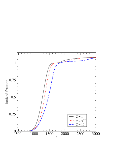
Figure 1: Ionization fraction $\bar{X_{e}}$ for a Universe with the preferred WMAP7-year cosmological parameters citeWMAP as a function of redshift for a homogeneous Universe (solid) and two Universes with small-scale inhomogeneities $\sqrt{\langle(\delta n/n)^{2}\rangle}=\sqrt{3}$ (dotted) and $10$ (dashed), respectively. Here, somewhat arbitrarily, the parameters $f_{V}^{i}=(0.567,0.33,0.1)$ and $\Delta^{i}=(0.1,1,6)$ for the first inhomogeneous model and $f_{V}^{i}=(0.663,0.33,0.04)$ and $\Delta^{i}=(0.1,1,168)$ for the second model have been chosen, where $f_{V}^{i}$ is the volume fraction filled with density $n^{i}=(1+\Delta^{i})\langle n\rangle$ of zone $i$.

A key observation in Eq. (7) is that it is non-linear in density in the first term on the RHS and in the factor $C$ remark3 . In an Universe inhomogeneous on scales $L\ll l_{\gamma}$ CMBR anisotropies depend on the average electron density $\langle n_{e}\rangle$. However, due to the non-linearity $\langle n_{e}\rangle\neq n_{e}^{\rm homo}$ where $n_{e}^{\rm homo}$ is the electron density in a homogeneous Universe, irrespective of the fact that the baryon density $n_{b}^{\rm homo}=\langle n_{b}\rangle$ equals the average baryon density in the inhomogeneous Universe. This may be seen in Fig. 1 where we computed with help of the public code RECFAST Seager:1999km the ionization fraction $\bar{X_{e}}=\langle n_{e}\rangle/\langle n_{H}\rangle\neq\langle X_{e}\rangle$ in a inhomogeneous Universe by taking the average of the electron densities of three independent regions remark4 with different baryonic densities but with the same average density as a homogeneous Universe. It is seen that the drop in $\bar{X_{e}}$, i.e. recombination, occurs earlier when inhomogeneities exist.

CMBR temperature anisotropies may be calculated at linear order by evolving temperature $\Theta_{0}$ and gravitational potential $\Psi$ perturbations of wavevector $k$ across the epoch of recombination. When this is done the observed temperature fluctuations are related to $\Theta_{0}+\Psi=({\hat{\Theta}}_{0}+\Psi){\cal D}(k)$ CMBR where

$${\cal D}(k)=\int_{0}^{\eta_{0}}{\rm d}\eta\frac{{\rm d}\tau}{{\rm d}\eta}\,{\rm e}^{-\tau(\eta,\eta_{0})}{\rm e}^{\bigl{[}k/k_{D}(\eta)\bigr{]}^{2}}$$ (9)

is due to the imperfect coupling of photons and baryons inducing exponential damping of perturbations on the photon diffusion scale $k_{D}(\eta)$, and $g({\eta}){\rm d}\eta={\rm d}\tau/{\rm d}\eta\,{\rm exp}(-\tau){\rm d}\eta$ is the fraction of photons observed today (i.e. at present conformal time $\eta_{0}$) which scattered last between conformal times $\eta$ and $\eta+{\rm d}\eta$, with $g({\eta})$ the visibility function. Here ${\rm d}\tau/{\rm d}\eta=X_{e}n_{H}\sigma_{Th}a$ with $\sigma_{Th}$ the Thomson cross section and $a$ scale factor, such that $\tau$ is the photon optical depth. The damping factor ${\cal D}(k)$ strongly modifies the undamped ${\hat{\Theta}}_{0}+\Psi$ temperature fluctuations. The behavior of ${\hat{\Theta}}_{0}$ is given by the solutions of the equation of a forced oscillator. It is well known that due to well specified initial conditions (i.e. only growing modes) ${\hat{\Theta}}_{0}(k)$ exhibits an oscillatory behavior with peaks given by $k_{m}r_{s}\simeq m\pi$ where $m$ is an integer. These peaks are due to perturbations having performed half, one, one-and-a-half, … sonic oscillations where

$$r_{S}=\int_{0}^{\eta_{\rm rec}}c_{s}\,{\rm d}\eta=\int_{z_{\rm rec}}^{\infty}c_{s}\frac{{\rm d}z}{H(z)}$$ (10)

is the sound horizon, with $\eta_{\rm rec}$ ($z_{\rm drec}$) conformal time (redshift) at recombination, $c_{s}$ the baryon-photon speed of sound, and $H$ the Hubble constant. Corresponding peaks in the temperature-temperature correlation function on angular scale, or equivalently on spherical harmonic multipole $l$, are observed at $l_{m}\simeq k_{m}(\eta_{0}-\eta_{\rm rec})$. The above gives us most of the ingredients to qualitatively understand modifications in the CMBR anisotropies from small scale inhomogeneity.

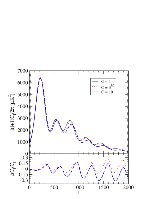
Figure 2: CMBR anisotropies in conventional units (cf. WMAP ) (upper panel) as a function of multipole for the best-fit WMAP7 year model, and the two inhomogeneous models described in the caption of Fig. 1, as well as their fractional differences (lower panel) to the best-fit WMAP7 year model. The same line coding as in Fig. 1 is applied.

We modified CAMB CAMB to compute the CMBR anisotropies when magnetic field induced baryon density fluctuations are present. The results are shown in Fig. 2 showing the anisotropies and their fractional deviations from the best-fit WMAP7 model for the two inhomogeneous Universes with $X_{e}$ shown in Fig. 1. It is seen that inhomogeneities have two main effects (a) they move the Doppler peak locations to higher multipoles and (b) they enhance Silk damping of the high $l$ peaks. Both may be understood by inspecting Fig. (1). In small-scale inhomogeneous Universes high density regions recombine earlier, making the average ionization fraction $X_{e}$ drop significantly earlier, and therefore increasing the redshift of ionization $z_{\rm rec}$. Low density regions which recombine later are not too important for the visibility function since they do not contain too many electrons. For example, for $\sqrt{\langle(\delta n/n)^{2}\rangle}=\sqrt{3}$ recombination (the peak of the visibility function) is moved from $z_{\rm rec}\approx 1078$ to $z_{\rm rec}\approx 1118$ a substantial change of $6.6\%$. In order to induce such a large change of $z_{\rm rec}$ by a change of the baryonic- or matter- densities, relative changes of $\sim 20\%$, $\sim 10\%$, respectively are required. These are far beyond the WMAP7 and baryonic acoustic oscillation (BAO) BAO error bars on their respective values of $\sim\pm 2\%$, and $\sim\pm 3.3\%$, respectively. An earlier recombination leads to Doppler peaks moving to higher $l$, e.g. for $\sqrt{\langle(\delta n/n)^{2}\rangle}=\sqrt{3}$ all lower peaks are moved by $\sim 2.5\%$. This may be understood since to lowest order $\Delta l\simeq\Delta z_{rec}^{1/2}$ (see below).

The second effect, enhanced Silk damping, is somewhat more surprising since the Silk damping scale is the diffusion scale (i.e. $d_{\gamma}\simeq\sqrt{l_{\gamma}t}$ with $l_{\gamma}$ photon mean free path and $t$ time) at recombination. Earlier recombination would imply less time for photon diffusion and so less Silk damping. However, inspecting again Fig. (1) one observes that in the inhomogeneous Universes $\langle X_{e}\rangle$ is smaller by $\sim 10\%$ already some time before recombination. This is due to earlier helium recombination in the high density regions. A smaller electron density implies larger $l_{\gamma}$ and therefore larger $d_{\gamma}$. As this latter effect dominates, the combined effect is more Silk damping as evident from Fig. (2).

Fractional changes in the CMBR anisotropies in inhomogeneous Universes compared to homogeneous Universes are substantial $\sim 10\%$ even for $\sqrt{\langle(\delta n/n)^{2}\rangle}\sim 1$, particular at high multipoles. On first sight one would think that such large changes may be detected or ruled out by the Planck mission. To good approximation $l_{m}\simeq k_{m}\eta_{0}\sim\eta_{0}/r_{S}\sim\eta_{0}/\eta_{\rm rec}\sim[H_{\rm rec}(1+z_{0})]/[H_{0}(1+z_{\rm rec})]$. Assume for the moment that the Universe only contains matter $\Omega_{M}h^{2}=\Omega_{d}h^{2}+\Omega_{b}h^{2}$ and radiation, where $\Omega_{d}$, $\Omega_{b}$ are dark matter- and baryon- contributions to the critical density today, and $h$ is the Hubble constant in units of $100{\rm km\,s^{-1}Mpc^{-1}}$. If one then assumes that the Universe is critically closed $l_{m}$ becomes a function of only $z_{\rm rec}$ (since $[H_{\rm rec}(1+z_{0})]/[H_{0}(1+z_{\rm rec})]\sim z_{\rm rec}^{1/2}$ up to calculable radiation contributions) independent of $\Omega_{M}$ or the Hubble constant. Since $z_{\rm rec}$ is only logarithmically dependent on well-know atomic physics, magnetic field induced density fluctuations could be detected/ruled out to very high precision via the shift of the Doppler peaks. Unfortunately the situation is somewhat more complicated as the present Universe is dominated by a cosmological constant. In that case $1/H_{0}\sim\eta_{0}=f_{1}(\Omega_{M}h^{2},\Omega_{\Lambda}h^{2})$ and $H_{\rm rec}=f_{2}(\Omega_{M}h^{2},z_{\rm rec})$ (using that the radiation density is well known), where $f_{i}$ are functions. To break possible degeneracies between density inhomogeneities and other cosmological parameters $\Omega_{M}h^{2}$ and $\Omega_{\Lambda}h^{2}$ must be known accurately. Here $\Omega_{M}h^{2}$ can be inferred from the CMBR anisotropies and $\Omega_{\Lambda}h^{2})$ from either supernovae surveys or BAO observations of the angular diameter distance. Nevertheless, it is not clear if one can achieve the desired accuracy. Alternatively, assuming a closed Universe and using a precise measurement of the Hubble constant $h$ could also lead to a fairly precise prediction of $z_{\rm rec}$ and the $l_{m}$’s. A more detailed analysis is beyond the scope of this letter and is deferred to a future publication.

Which field strengths are detectable in case the Planck mission combined with other surveys will be able to establish (or refute) the existence of small-scale inhomogeneity before recombination remark6 ? Following Ref. BJ04 primordial magnetic fields do decay on the scale implicitly given by $v/L\simeq H$, with $v\simeq v_{A}^{2}/L\alpha$ before recombination in the viscous regime and $v\simeq v_{A}$ after in the turbulent regime. Assuming that the initial spectrum is given by $B\sim L^{-n/2}$ one may deduce that magnetic field strength shortly before, $B^{<}$ and after $B^{>}$ recombination (which is also the final present day field strength BJ04 ) are related by $B^{<}\simeq(\alpha/H_{\rm rec})^{n/(2n+4)}B^{>}$. That is, due to the rapid disappearance of photon drag during recombination, substantial amounts of magnetic field energy density dissipates right at recombination since $\alpha/H_{\rm rec}\approx 170$. It is not clear, but subject to further investigation, if shocks resulting from the magnetic stress acceleration and the accompanying shock ionization during recombination are also of importance. In any case, for a final magnetic field strength of $B^{>}\simeq 10^{-11}{\rm Gauss}$ and a white noise spectral index $n=3$ one finds $B^{<}\simeq 4.7\times 10^{-11}$Gauss which comes close to fulfilling $v_{A}\sim c_{s}$ such that it should be potentially detectable.

In summary, we have argued that primordial magnetic fields induce small-scale baryon inhomogeneity of substantial amplitude. Due to non-linearities in the recombination equations such inhomogeneity induces changes in the ionization fraction before recombination. This, in turn, influences the anisotropies in the CMBR, such that present day primordial magnetic fields of strength $B\sim 10^{-11}$ Gauss could potentially be detected by a combination of future and present CMBR, BAO, and supernovae observations.

Acknowledgments We acknowledge a useful discussion with Levon Pogosian.

References

- (1) A. Neronov and I. Vovk, Science 328, 73 (2010); F. Tavecchio, G. Ghisellini, L. Foschini, G. Bonnoli, G. Ghirlanda and P. Coppi, Mon. Not. Roy. Astron. Soc. 406, L70 (2010); K. Takahashi, M. Mori, K. Ichiki and S. Inoue, arXiv:1103.3835 [astro-ph.CO].
- (2) K. Dolag, M. Kachelriess, S. Ostapchenko and R. Tomas, Astrophys. J. 727, L4 (2011).
- (3) A. E. Broderick, P. Chang, C. Pfrommer, arXiv:1106.5494.
- (4) A. Kosowsky and A. Loeb, Astrophys. J. 469, 1 (1996); K. Subramanian and J. D. Barrow, Phys. Rev. Lett. 81, 3575 (1998); R. Durrer, P. G. Ferreira and T. Kahniashvili, Phys. Rev. D 61, 043001 (2000); A. Mack, T. Kahniashvili and A. Kosowsky, Phys. Rev. D 65, 123004 (2002); C. Caprini, R. Durrer and T. Kahniashvili, Phys. Rev. D 69, 063006 (2004); A. Lewis, Phys. Rev. D 70, 043011 (2004); D. Yamazaki, K. Ichiki, T. Kajino and G. J. Mathews, Astrophys. J. 646, 719 (2006); M. Giovannini and K. E. Kunze, Phys. Rev. D 77, 123001 (2008); F. Finelli, F. Paci and D. Paoletti, Phys. Rev. D 78, 023510 (2008); T. R. Seshadri and K. Subramanian, Phys. Rev. Lett. 103, 081303 (2009); M. Shiraishi, D. Nitta, S. Yokoyama, K. Ichiki and K. Takahashi, Phys. Rev. D 83, 123003 (2011); L. Pogosian, A. P. S. Yadav, Y. F. S. Ng and T. Vachaspati, arXiv:1106.1438.
- (5) K. Jedamzik, V. Katalinic and A. V. Olinto, Phys. Rev. Lett. 85, 700 (2000).
- (6) All cited length scales and magnetic field strengths in this paper are comoving, i.e. the values they would have at the present epoch are given.
- (7) R. Banerjee and K. Jedamzik, Phys. Rev. D 70, 123003 (2004)
- (8) K. Jedamzik and G. Sigl, Phys. Rev. D 83, 103005 (2011).
- (9) R. Durrer and C. Caprini, JCAP 0311, 010 (2003).
- (10) K. Jedamzik, V. Katalinic and A. V. Olinto, Phys. Rev. D 57, 3264 (1998).
- (11) Due to efficient CMBR cooling the effective speed of sound is that for an isothermal baryon gas.
- (12) K. Subramanian and J. D. Barrow, Phys. Rev. D 58, 083502 (1998).
- (13) P.J.E. Peebles Principles of Physical Csomology, Princeton University Press 1976.
- (14) In fact, the nonlinearity in is only very mild since may be well approximated by signifying that double photon decay is about one order of magnitude more important than Lyman- transitions in producing neutral hydrogen in the ground state.
- (15) E. Komatsu et al. [WMAP Collaboration], Astrophys. J. Suppl. 192, 18 (2011).
- (16) S. Seager, D. D. Sasselov and D. Scott, Astrophys. J. Suppl. 128, 407 (2000)
- (17) Though the Lyman- photon mean free path is coincidentally of the order of kpc, i.e. different dense regions are not completely decoupled from each other, the “independent region” approximation is very good since hydrogen formation by Lyman- transitions is subdominate (cf. remark3 ).
- (18) W. Hu and N. Sugiyama, Astrophys. J. 444, 489 (1995); C. P. Ma and E. Bertschinger, Astrophys. J. 455, 7 (1995).
- (19) A. Lewis, A. Challinor and A. Lasenby, Astrophys. J. 538, 473 (2000).
- (20) W. J. Percival, S. Cole, D. J. Eisenstein, R. C. Nichol, J. A. Peacock, A. C. Pope and A. S. Szalay, Mon. Not. Roy. Astron. Soc. 381, 1053 (2007).
- (21) There are no other plausible candidats for re-creating small-scale inhomogeneity after Silk damping which is volume filling and of magnitude known to the authors.