Instabilities of Bosonic Spin Currents in Optical Lattices

Abstract

We analyze the dynamical and energetic instabilities of spin currents in a system of two-component bosons in an optical lattice, with a particular focus on the Neel state. We consider both the weakly interacting superfluid and the strongly interacting Mott insulating limits as well as the regime near the superfluid-insulator transition and establish the criteria for the onset of these instabilities. We use Bogoliubov theory to treat the weakly interacting superfluid regime. Near the Mott transition, we calculate the stability phase diagram within a variational Gutzwiller wavefunction approach. In the deep Mott limit we discuss the emergence of the Heisenberg model and calculate the stability diagram within this model. Though the Bogoliubov theory and the Heisenberg model (appropriate for deep superfluid and deep Mott phase respectively) predict no dynamical instabilities, we find, interestingly, between these two limiting cases there is a regime of dynamical instability. This result is relevant for the ongoing experimental efforts to realize a stable Neel-ordered state in multi-component ultracold bosons.

I Introduction

Ultracold atomics gases have recently emerged as a very important platform to study non-equilibrium quantum dynamics of interacting many-body systems. The tunability of Hamiltonian parameters together with almost complete isolation from the environment and the long time-scales in these systems have made it possible to study intrinsic non-equilibrium dynamics of these systems without ultrafast probes. Recently, there has been a growing number of experimental and theoretical investigations of the dynamical properties of Bose-Einstein Condensates (BECs) in optical lattices Morsch and Oberthaler (2006). Of particular interest are experiments which exhibit a dynamical instability, which is a generic phenomenon present in nonlinear systems under appropriate conditions. Previously established examples of dynamical instabilities occur in water waves Whitham (1965); Benjamin and Hasselmann (1967), light in dielectric media Ostrovskii (1964, 1967); Hasegawa and Brinkman (1980); Tai et al. (1986), and plasmas Hasegawa (1972); Pesme et al. (1988); McKinstrie and Bingham (1989). Recently, dynamical instabilities have been observed in ultracold fermi gases after a tuning of the interaction parameters Jo et al. (2009); Pekker et al. (2011). The realization of dynamical instabilities for current-carrying states in BECs have received considerable attention both theoretically Wu and Niu (2001); Konotop and Salerno (2002); Smerzi et al. (2002); Machholm et al. (2003); Modugno et al. (2004); Altman et al. (2005); Polkovnikov et al. (2005) as well as experimentally Raman et al. (1999); Cataliotti et al. (2003); Fallani et al. (2004); Anker et al. (2005); Fertig et al. (2005); De Sarlo et al. (2005); Mun et al. (2007); Ferris et al. (2008).

Two qualitatively distinct types of instabilities can occur for interacting systems of bosons: (i) the energetic instability and (ii) the dynamical instability. The energetic instability occurs if the system is not at a local minimum of the mean-field energy. If the system is capable of dissipating energy, then it will decay from the initial metastable state thereby exhibiting the instability. A well-known example for this case is the Landau instability (LI) for which a superfluid carrying current in excess of the sound velocity becomes unstable, leading to a breakdown of superfluidity. In contrast, a dynamical instability (DI) occurs when the system has collective modes with complex frequencies. Such modes will result in an exponential growth of small perturbations which manifests as a rapid depletion and fragmentation of the condensate Fallani et al. (2004); Ferris et al. (2008). For systems that do not have a dissipative mechanism, the energetic instability alone will not occur. On the other hand, the dynamical instability occurs even without dissipation, and will be observable unless the growth time of the most unstable mode is longer than experimental time scales. It can also be seen that an energetic instability is a necessary condition for a dynamical instability.

Bosons in an optical lattice undergo a quantum phase transition from a superfluid phase in the weakly interacting limit to an incompressible Mott insulator phase as the interaction parameter increases beyond a critical value. Scalar bosonic condensates have a U(1) symmetry associated with the superfluid phase, resulting in a conserved mass current. In the presence of a lattice, when the externally imposed current exceeds a critical value, the system manifests a dynamical instability Wu and Niu (2001); Konotop and Salerno (2002); Smerzi et al. (2002). The critical current required for the dynamical instability decreases with increasing interaction strength and vanishes at the critical interaction required for the superfluid-insulator transition. Additional types of dynamical instabilities can occur in multicomponent condensates due the their more complex order parameters. In this paper we will focus on two-component bosons in an optical lattice with spin-independent interactions. In addition to the superfluid-insulator transition, this system also shows a spontaneous ferromagnetic spin ordering in the equilibrium ground state. This system has an SU(2) symmetry due to invariance of the energy under spin rotation which results in a conserved spin current. In the presence of externally imposed spin currents (spin twists), the system exhibits dynamical instabilities when the spin current exceeds a critical value. We will mainly focus on these spin-current driven instabilities, which occur in addition to and even in the absence of any mass current driven instabilities.

Previous work addressing spin current instabilities in bosonic systems have focused on the continuum, weakly interacting superfluids where the Gross-Pitaevskii Equation (GPE) is applicable. In such a context, the counterflow instability Law et al. (2001); Kuklov and Svistunov (2003); Takeuchi et al. (2010); Hoefer et al. (2010); Hamner et al. (2011) as well as the instability of a spin-one condensate from an initial helical state Vengalattore et al. (2008); Cherng et al. (2008) have been investigated. Here we analyze the instabilities of the system in the presence of an optical lattice for a wide range of interaction parameters going from the weakly interacting limit (the deep superfluid phase) through the intermediate regime near the superfluid-insulator transition to the strongly interacting (atomic) limit, deep into the Mott phase. The weakly interacting regime is treated within the standard Bogoliubov theory, while the strongly interacting regime is treated within a spin-wave approximation of the ferromagnetic Heisenberg model, where the spin-spin interaction comes from super-exchange mechanism. The intermediate interaction regime is treated within a variational Gutzwiller wavefunction ansatz. We extend the Gutzwiller ansatz to both the deep superfluid and the deep Mott limit and compare the results with those from the more established formalisms mentioned above.

To analyze stability of the bosonic states, we construct either mass or spin current carrying mean-field states. The spectrum of quantum fluctuations about these stationary states is then calculated within a Gaussian approximation. Negative eigenvalues of the fluctuation Hamiltonian indicate an energetic instability while a complex collective mode spectrum indicates a dynamical instability. For a dynamical instability, the positive imaginary part of the complex spectrum gives the growth rate of the unstable fluctuation modes. Our main results are: (i) We show that the mass current induced instabilities give rise to the same instability phase diagram in the critical current interaction plane for both spinless and two-component bosons. (ii) The two-component bosons exhibit a spin-current induced dynamical instability in a large region of the critical current interaction strength plane in the superfluid phase. We also show the collective modes which are unstable and compute their growth rates. (iii) We focus on the Neel-ordered state, which can be interpreted as a spin-current-carrying state with particular commensurate wavevector. Although the Neel configuration is not the ground state of the system, there are proposals Sørensen et al. (2010) to experimentally explore the physics about this high energy state provided its lifetime is sufficiently long. We show that while this state is stable in the deep superfluid and insulating limits, in the intermediate regime, interestingly, the system is dynamically unstable. We thus provide a comprehensive picture of the spin-current induced dynamical instabilities in two-component bosons on optical lattices for a wide range of interactions and spin currents.

The paper is organized as follows. In Sec. II, we review the established DI of the mass current of spinless bosons. We use the Bogoliubov theory to analyze the superfluid limit and the Gutzwiller ansatz to analyze the strongly-interacting regime close to Mott boundary. This prepares us to investigate the instabilities related to the spin current of a two-component Bosonic condensate in Sec. III in the regime of weak as well as intermediate interactions. We shall present the stability phase diagram and discuss how our results are connected to the deep Mott limit. In Sec. IV we discuss the stability of the Neel state limit for different regimes. Finally in Sec. V we summarize our results.

II Instabilities of moving scalar condensates

For completeness and to set the notation and general approach, we first briefly consider the mass current in a single-component BEC and the concomitant Landau and dynamical instabilities. The weakly interacting superfluid case was originally considered in Refs. Smerzi et al. (2002); Wu and Niu (2001), while the regime near the Mott transition was addressed in Ref. Altman et al. (2005); Polkovnikov et al. (2005). A system of bosons on a lattice and in the lowest band is described by the Bose-Hubbard model

$$H=-t\sum_{\left\langle ij\right\rangle}\left(b_{i}^{\dagger}b_{j}+\mathrm{hc}\right)+\frac{U}{2}\sum_{i}\left(n_{i}-\bar{n}\right)^{2}-\mu\sum_{i}\left(n_{i}-\bar{n}\right)$$ (1)

where $b^{\dagger}_{i}$ is the boson creation operator on the lattice site $i$, $t$ is the hopping matrix element, $U$ is the on-site repulsion, $\mu$ is the chemical potential, $n_{i}=b^{\dagger}_{i}b_{i}$, and $\bar{n}$ is the average number of bosons per site. We consider this model in one, two, and three dimensions for cubic lattices. When $t\gg U/\bar{n}$ the system has a superfluid ground state, and Bogoliubov theory describes its elementary excitations. When $t\sim U/\bar{n}$, there is a quantum phase transition at $U=U_{c}$ to an incompressible Mott state. The Bogoliubov theory fails in the vicinity of this transition, however, a variational Gutzwiller ansatz can be used to treat the system in this regime.

II.1 Weakly Interacting Superfluid

Deep in the superfluid phase the current-carrying states can be represented by a condensate wavefunction of the form

$$\bar{b}_{i}=\sqrt{n}e^{i\mathbf{p}\cdot\mathbf{x}_{i}}.$$ (2)

which has a phase twist along $\hat{p}$ and carries a mass current $\propto\sin\bf{p\cdot\bf{x_{ij}}}$ between neighboring sites. This wavefunction can be found within mean-field theory by solving the Gross-Pitaevskii equation. Expanding the energy of the system, Eq. (1), about this state to quadratic order, with $b_{i}=\bar{b}_{i}+\phi_{i}$, one obtains the fluctuation Hamiltonian $\delta H=\sum_{\mathbf{k}}\Phi_{\mathbf{k}}^{\dagger}M_{\mathbf{k}}(\mathbf{p})\Phi_{\mathbf{k}}$ where $\Phi_{\mathbf{k}}^{\dagger}=\left(\phi_{\mathbf{k}}^{\dagger},\phi_{-\mathbf{k}}\right)$ and

$$M_{\mathbf{k}}=\left(\begin{array}[]{cc}\epsilon_{\mathbf{k}+\mathbf{p}}-\epsilon_{\mathbf{p}}+Un&Un\\ Un&\epsilon_{\mathbf{k}-\mathbf{p}}-\epsilon_{\mathbf{p}}+Un\end{array}\right)$$ (3)

with $\epsilon_{\mathbf{q}}=-zt\gamma_{\mathbf{q}}$, where $z$ is the coordination number and $\gamma_{\mathbf{q}}=z^{-1}\sum_{\mathbf{\delta}}e^{i\mathbf{q}.\mathbf{\delta}}$. The energies of the normal modes of the system are given by the eigenvalues of the matrix $\sigma_{z}M_{\mathbf{k}}$ Wu and Niu (2001) where $\sigma_{z}$ is a Pauli matrix. On the other hand, if the system is at a local minimum in energy, then the matrix $M_{\mathbf{k}}$ itself will be positive definite. We thus summarize the following criteria for the instabilities:

• LI: at least one eigenvalue of $M_{\mathbf{k}}$ is negative

• DI: at least one eigenvalue of $\sigma_{z}M_{\mathbf{k}}$ is complex

For mass-current-carrying states, it is well known that the continuum theory only sustains Landau instabilities, which occur when the current in the system exceeds the speed of sound. There are no dynamical instabilities in the continuum theory. However, on a lattice the system exhibits both Landau and dynamical instabilities with the criterion for critical current summarized in Table 1. The dynamical instability is crucially related to the softening of collective modes at finite wavevectors, which does not occur in the continuum.

	Phase twist		Spin Twist
	Continuum	Lattice	Continuum	Lattice
LI	$\tilde{p}>\sqrt{mUn}$	$\frac{\sin^{2}\tilde{p}}{\cos\tilde{p}}>\frac{Un}{zt}$	$\tilde{p}\neq 0$	$\tilde{p}\neq 0\,\mathrm{mod}\,2\pi$
DI	Never	$\cos\tilde{p}<0$	$\tilde{p}\neq 0$	$\tilde{p}\neq 0,\pm\frac{\pi}{2}\,\mathrm{mod}\,2\pi$

Table 1: The conditions for Landau and dynamical instabilities of mass-current carrying states (for spinless bosons) and spin-current carrying states (for 2-component spin-full bosons) in the weakly interacting limit on a square lattice (calculated within Bogoliubov theory). The results are valid for one, two, and three dimensions. The case of twisting along the diagonal of the square lattice: $\mathbf{p}=\tilde{p}\sum_{i}\hat{x}_{i}$ is taken. For comparison, the conditions for the instabilities in the continuum are also given.

II.2 Gutzwiller Ansatz

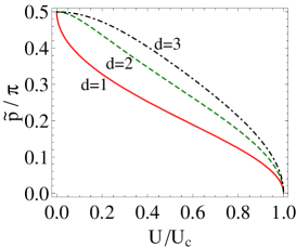
Figure 1: Stability phase diagram of phase twists in a lattice in different dimensions, where twisting is imposed along: $\mathbf{p}=\tilde{p}\hat{x}$. The same diagram is obtained for either spinless bosons Eq. (1) or the two-component bosons Eq. (5). This diagram agrees well with the more extensive treatment presented in Altman et al. (2005); Polkovnikov et al. (2005).

To investigate the DI for the Bose-Hubbard model for stronger interactions, we shall approach the problem within a truncated Hilbert space. We consider the variational Gutzwiller wavefunction for the ground state, $\left|\Omega\right\rangle=\prod_{i}\left|\Omega_{i}\right\rangle$, with $\left|\Omega_{i}\right\rangle=\cos\frac{\theta_{i}}{2}\left|\bar{n}\right\rangle_{i}+e^{i\eta_{i}}\sin\frac{\theta_{i}}{2}\left[\cos\frac{\chi_{i}}{2}e^{-i\varphi_{i}}\left|\bar{n}-1\right\rangle_{i}+\sin\frac{\chi_{i}}{2}e^{i\varphi_{i}}\left|\bar{n}+1\right\rangle_{i}\right]$, where $\left|n\right\rangle_{i}$ are the Fock states on the site $i$. This variational state was used in Ref. Altman and Auerbach (2002) to study the Bose-Hubbard model near the Mott transition in the absence of a current. Our calculations follow along similar lines with an important distinction: the phase $\varphi_{i}$ is position-dependent, i.e. $\varphi_{i}=\mathbf{p}\cdot\mathbf{x}_{i}$ such that $\left\langle\Omega\right|b_{i}\left|\Omega\right\rangle\propto\sin\theta e^{i\mathbf{p}\cdot\mathbf{x}_{i}}$, which ensures that the state carries a mass current flowing along $\hat{p}$. Other parameters are then varied to minimize the energy of this mean-field state, giving $\chi=\frac{\pi}{2}$ and $\eta=0$.

The Hamiltonian is expanded about this stationary state in the following way: we introduce the bosonic pseudospin operators $t_{\alpha i}^{\dagger}\left|\mathrm{vac}\right\rangle\equiv\left|\bar{n}+\alpha\right\rangle_{i}$, $\alpha=\{-1,0,1\}$ with the constraint $\sum_{\alpha}t_{\alpha i}^{\dagger}t_{\alpha i}=1$, so that the Boson operators can be written as $b_{i}^{\dagger}\rightarrow\sqrt{\bar{n}}t_{0i}^{\dagger}t_{-1i}+\sqrt{\bar{n}+1}t_{1i}^{\dagger}t_{0i}$. A unitary transformation is then performed with

$$\left(\begin{array}[]{c}d_{0i}^{\dagger}\\ d_{1i}^{\dagger}\\ d_{2i}^{\dagger}\end{array}\right)=\left(\begin{array}[]{ccc}\frac{e^{-i\mathbf{p}\cdot\mathbf{x}_{i}}}{\sqrt{2}}\sin\frac{\theta}{2}&\cos\frac{\theta}{2}&\frac{e^{i\mathbf{p}\cdot\mathbf{x}_{i}}}{\sqrt{2}}\sin\frac{\theta}{2}\\ -\frac{e^{-i\mathbf{p}\cdot\mathbf{x}_{i}}}{\sqrt{2}}\cos\frac{\theta}{2}&\sin\frac{\theta}{2}&-\frac{e^{i\mathbf{p}\cdot\mathbf{x}_{i}}}{\sqrt{2}}\cos\frac{\theta}{2}\\ \frac{e^{-i\mathbf{p}\cdot\mathbf{x}_{i}}}{\sqrt{2}}&0&-\frac{e^{i\mathbf{p}\cdot\mathbf{x}_{i}}}{\sqrt{2}}\end{array}\right)\left(\begin{array}[]{c}t_{-1i}^{\dagger}\\ t_{0i}^{\dagger}\\ t_{1i}^{\dagger}\end{array}\right)$$ (4)

and the Hamiltonian is written in terms of the $d$ operators. Since $d_{0}^{\dagger}\left|\mathrm{vac}\right\rangle$ represents the minimum energy state, it is macroscopically occupied, while $d_{n>0}^{\dagger}$ are fluctuations about this state. Therefore, we eliminate $d_{0}^{\dagger}$ using $d_{0}^{\dagger}\approx d_{0}\approx 1-\frac{1}{2}d_{1i}^{\dagger}d_{1i}-\frac{1}{2}d_{2i}^{\dagger}d_{2i}$, which resembles the Holstein-Primakoff transformation Holstein and Primakoff (1940) used in spin models.

To the quadratic order in the operators $d_{n>0}^{\dagger}$, the Hamiltonian has the form $H=\Psi^{\dagger}_{{\bf k}}M_{{\bf k}}\Psi_{{\bf k}}$ where $\Psi^{\dagger}_{{\bf k}}\equiv\left(d_{1k}^{\dagger},d_{1,-k},d_{2k}^{\dagger},d_{2,-k}\right)$ and the form of $M_{{\bf k}}$ is given in Appendix A. For a given $U/t$ and $\mathbf{p}$, we compute the energies $\omega_{1,2k}$ for $k\in\left[-\pi,\pi\right]$ by a Bogoliubov transformation. As noted before, the presence of complex eigenfrequencies indicate a dynamical instability.

For direct comparison with previous work, we consider $\mathbf{p}$ along an axis of a $d$-dimensional cubic lattice $\left(\mathbf{p}=p\hat{x}_{1}\right)$, giving $\gamma_{\mathbf{p}}=\frac{\cos p+(d-1)}{d}$. The resulting phase diagram is shown in Fig. 1, which shows good agreement with the results in Altman et al. (2005); Polkovnikov et al. (2005) where a numerical analysis is performed, taking a larger Hilbert space.

The Bogoliubov analysis is justified only if the fluctuation occupation $\left\langle d_{1i}^{\dagger}d_{1i}+d_{2i}^{\dagger}d_{2i}\right\rangle$ is small compared to unity. This is checked in the stable regimes after the Bogoliubov transformation is done. We find that for the 2D system, the fluctuation is less than $0.2$ for all $U>0.1U_{c}$ and reach up to $0.5$ as $U\rightarrow 0$ and $p\rightarrow\pi/2$. This means the quantitative result should be trustworthy for $U>0.1U_{c}$. However in 1D we always find divergent occupation of the fluctuations as expected because of the significance of quantum fluctuations. The qualitatively good agreement for 1D results with experiment might be understood as due to the logarithmic nature of the divergence, which is not severe in finite-sized systems.

III Spin Current Instabilities in Two-Component Condensates

Having set up the formalism to study Landau and dynamical instabilities in spinless bosonic systems, we will now adapt this formalism to study instabilities of spin-current carrying states in condensates of two-component bosons. The starting point for our analysis is the two-component rotationally invariant Bose-Hubbard model

$$H = -t\sum_{\left\langle ij\right\rangle\sigma}\left(b_{i\sigma}^{\dagger}b_{j\sigma}+\mathrm{hc}\right)+\frac{U}{2}\sum_{i}\left(n_{i}-\bar{n}\right)^{2}$$ (5)

$$-\mu\sum_{i}\left(n_{i}-\bar{n}\right).$$

where $b^{\dagger}_{i\sigma}$ creates a boson of spin $\sigma$ on site $i$, $n_{i}=\sum_{\sigma}b_{i\sigma}^{\dagger}b_{i\sigma}$, and $\bar{n}$ is the average particle number per site. Such a system could be realized using, for instance, two hyperfine states of alkali atoms. Due to the smallness of spin-exchange interaction for typical alkali atoms, such systems possess an approximate SU(2) symmetry, which is reflected in the spin-independent form of the interactions which we consider here. For simplicity we will concentrate on the case when $\bar{n}=1$ except for the Bogoliubov analysis.

The weakly interacting superfluid phase (first considered in Ref. Law et al. (2001)) of the spinfull bosons is described by the Bogoliubov theory around a mean-field state with a two-component condensate wavefunction. The intermediate interaction regime near the Mott transition is analyzed, as before, with a variational Gutzwiller ansatz, albeit with an extended local Hilbert space. However, unlike the spinless bosons, the ferromagnetic spin-spin interaction in the deep Mott phase, arising out of a super-exchange mechanism, is not captured by the simple Gutzwiller ansatz. To treat this limit, we work with a ferromagnetic Heisenberg model with a spin-spin interaction $J=4t^{2}/U$ and analyze the spin-current induced instabilities within a spin-wave formalism.

III.1 Weakly interacting Superfluid

The weakly interacting superfluid regime admits coherent mean-field spin current-carrying solutions of the form

$$\mathbf{\bar{b}}_{i}=e^{i\sigma^{x}\mathbf{p}\cdot\mathbf{x}_{i}/2}\left(\begin{array}[]{c}\sqrt{n}\\ 0\end{array}\right).$$ (6)

Such states have a spin twist of ${\bf p}$, and carry spin current $\propto\sin\mathbf{p}\cdot\mathbf{x}_{ij}$ between neighbors. Expanding Eq. (5) about this stationary state to second order in quantum fluctuations, $b_{i\sigma}=\bar{b}_{i\sigma}+\phi_{i\sigma}$, gives the Hamiltonian $\delta H=\sum_{\mathbf{k}>0}\Phi_{\mathbf{k}}^{\dagger}M_{\mathbf{k}}\Phi_{\mathbf{k}}$ where $\Phi_{\mathbf{k}}^{\dagger}=\left(\phi_{\uparrow\mathbf{k}}^{\dagger},\phi_{\uparrow-\mathbf{k}},\phi_{\downarrow\mathbf{k}}^{\dagger},\phi_{\downarrow-\mathbf{k}}\right)$ and

$$M_{\mathbf{k}} = \left(\begin{array}[]{cccc}\xi+2Un&Un&\epsilon_{-}&0\\ Un&\xi+2Un&0&-\epsilon_{-}\\ \epsilon_{-}&0&\xi+Un&0\\ 0&-\epsilon_{-}&0&\xi+Un\end{array}\right)$$ (11)

where

$$\xi = \epsilon_{+}-\mu$$

$$\epsilon_{\pm} = \frac{\epsilon_{\mathbf{k}+\mathbf{p}/2}\pm\epsilon_{\mathbf{k}-\mathbf{p}/2}}{2}$$

with $\epsilon_{\mathbf{q}}=-zt\gamma_{\mathbf{q}}=-2t\sum_{i}\cos q_{i}$. For given $U$ and $\mathbf{p}$, negative eigenvalues of $M_{\mathbf{k}}$ for some $\mathbf{k}$ indicates LI while imaginary eigenvalues of $\sigma M_{\mathbf{k}}$ indicates DI, where $\sigma=\mathrm{diag}\left(1,-1,1,-1\right)$.

From here on, we will restrict ourselves to the case of spin currents along the diagonal of a square lattice: $\mathbf{p}=\tilde{p}\left(\hat{x}+\hat{y}\right)$ (for example $\tilde{p}=\pi$ represents the Neel state). The conditions for instabilities are summarized in Table 1. The LI is always present for any non-zero pitch, while DI is always present except for the $\tilde{p}=0$ ferromagnetic state and the $\tilde{p}=\pi$ Neel state.

To obtain a better understanding of the DI, we plot the wavevectors of the unstable modes, obtained from the Bogoliubov theory, as a function of the spin twist $\tilde{p}$ in the left column of Fig. 2. Here we consider wavevectors parallel to spin current ($\mathbf{k}\parallel\mathbf{p}$) for several values of $U$. Light gray areas indicate presence of LI but not DI, and dark areas indicate the presence of both LI and DI. The ferromagnetic state is always energetically and dynamically stable, as expected, while the Neel state has a LI but not a DI. With increasing $U$ the region where the DI is present increases, i.e. more and more wavevectors become unstable. However, the region where LI is present is almost independent of $U$.

The dispersions of the lowest collective modes ($\mathbf{k}\parallel\mathbf{p}$) for three special states, the ferromagnetic state ($\tilde{p}=0$), the Neel state ($\tilde{p}=\pi$) and the spin spiral state with a wavelength of $4$ lattice spacings ($\tilde{p}=\pi/4$), are plotted in the left column of Fig. 3. For the ferromagnetic state, there are two low energy modes: a charge mode related to the U(1) symmetry breaking, which disperses linearly and a spin mode related to the SU(2) symmetry breaking, which disperses quadratically, both of which are stable modes. As a spin current is imposed, the charge mode remains stable while the spin mode develops a DI near $k=0$, indicated by the thin red line. As we reach the Neel state, both the charge and the spin mode disperse linearly and are stable. Thus the DI disappears for the Neel state, which is stable in the weakly interacting limit. However, states with spin twists close to but not equal to $\pi$, are unstable with the instability being seeded around the wavevector $\mathbf{k}=\pi$.

III.2 Gutzwiller Ansatz

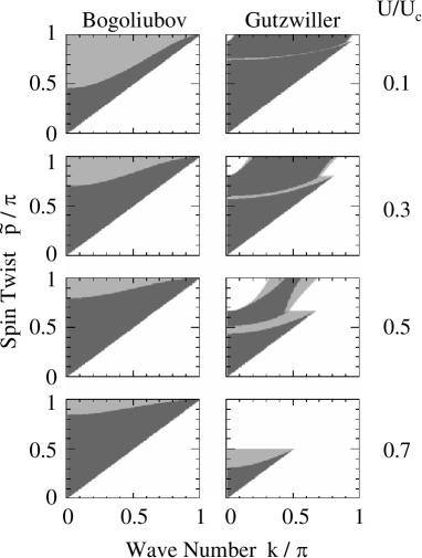
Figure 2: Diagrams showing regions of unstable modes for BEC spin-current-carrying state in optical lattice, analyzed with Bogoliubov theory (left column) and Gutzwiller ansatz (right column). The value of $U/U_{c}$ used is (from top to bottom) $0.1$, $0.3$, $0.5$, $0.7$. The spin twist plotted is from ferromagnetic state (${\bf p}=(0,0)$) to Neel state (${\bf p}=(\pi,\pi)$). $k$ is the wave vector of the normal mode. The shaded area indicates a LI (negative excitation energy), while dark shaded area indicates a DI (complex frequencies). The left column was previously obtained in Ref. Law et al. (2001).

To investigate the regime near the insulator-superfluid transition we adopt the Gutzwiller approach of Sec. II. For simplicity, we restrict ourselves to the case of unity filling. Then there are minimally six basis states per site that need to be included in the local Hilbert space: $\left\{\left|0\right\rangle,\left|\uparrow\right\rangle,\left|\downarrow\right\rangle,\left|\uparrow\uparrow\right\rangle,\left|\uparrow\downarrow\right\rangle,\left|\downarrow\downarrow\right\rangle\right\}$, where the last three states have double occupancy. The local Gutzwiller wavefunction is then parametrized in terms of ten variables (site indices omitted)

$$\left|\Omega\right\rangle = \sin\frac{\theta}{2}\cos\frac{\theta_{2}}{2}\left|0\right\rangle+e^{i(\varphi_{0}+\varphi_{1})}\cos\frac{\theta}{2}\cos\frac{\theta_{1}}{2}\left|\uparrow\right\rangle$$ (12)

$$+e^{i(\varphi_{0}-\varphi_{1})}\cos\frac{\theta}{2}\sin\frac{\theta_{1}}{2}\left|\downarrow\right\rangle$$

$$+e^{2i(\varphi_{2}+\varphi_{4})}\sin\frac{\theta}{2}\sin\frac{\theta_{2}}{2}\cos\frac{\theta_{3}}{2}\cos\frac{\theta_{4}}{2}\left|\uparrow\uparrow\right\rangle$$

$$+e^{2i(\varphi_{2}+\varphi_{3})}\sin\frac{\theta}{2}\sin\frac{\theta_{2}}{2}\sin\frac{\theta_{3}}{2}\left|\uparrow\downarrow\right\rangle$$

$$+e^{2i(\varphi_{2}-\varphi_{4})}\sin\frac{\theta}{2}\sin\frac{\theta_{2}}{2}\cos\frac{\theta_{3}}{2}\sin\frac{\theta_{4}}{2}\left|\downarrow\downarrow\right\rangle.$$

A phase twist $\left(\left\langle b_{\sigma}\right\rangle\propto e^{i\mathbf{p}\cdot\mathbf{x}}\right)$ can be imposed by setting $\varphi_{0}=\varphi_{2}=\mathbf{p}\cdot\mathbf{x}$ and other $\varphi_{i\neq 0,2}$ to be uniform; while a spin twist $\left(\left\langle S^{+}\right\rangle\propto e^{i2\mathbf{p}\cdot\mathbf{x}}\right)$ can be imposed by setting $\varphi_{1}=\varphi_{4}=\mathbf{p}\cdot\mathbf{x}/2$ and other $\varphi_{i\neq 1,4}$ to be uniform. Note that, in our parametrization, the spin-current-carrying states do not have any mass current, i.e. it is a state where the two spin species carry equal mass currents in the opposite direction. We find that a mass current produces a stability diagram identical to that of the spinless condensate in Sec. II. From now on we will concentrate on the case of spin twist only.

With a spin twist imposed on $\left|\Omega\right\rangle$, we expand the Hamiltonian around its stationary state and investigate the behavior of the fluctuation Hamiltonian. The full derivation is carried out in Appendix B. Here we shall present the results, concentrating on the case where the spin current is put along the diagonal: $\mathbf{p}=\tilde{p}\sum_{i}\hat{x}_{i}$. For comparison with the Bogoliubov theory, we plot in the right column of Fig. 2 the wavenumber of the unstable wavevectors (parallel to the spin current) as a function of the spin twist for different interaction strengths. We find that, contrary to the Bogoliubov theory, the region of unstable wavevectors decreases with increasing interaction within the Gutzwiller formalism. For example, the state at $U/U_{c}=0.7$ with $\tilde{p}>\pi/2$ is stable in the Gutzwiller formalism while it shows instability within the Bogoliubov theory. The Bogoliubov theory, which is accurate in the weakly interacting regime, thus overestimates the dynamical instability in the intermediate regime.The main qualitative difference, however, is in the stability of the Neel state ($\tilde{p}=\pi$). While the Bogoliubov theory predicts only a LI and no DI for this state, the Gutzwiller ansatz shows that the Neel state can be dynamically unstable in the intermediate interaction regime.

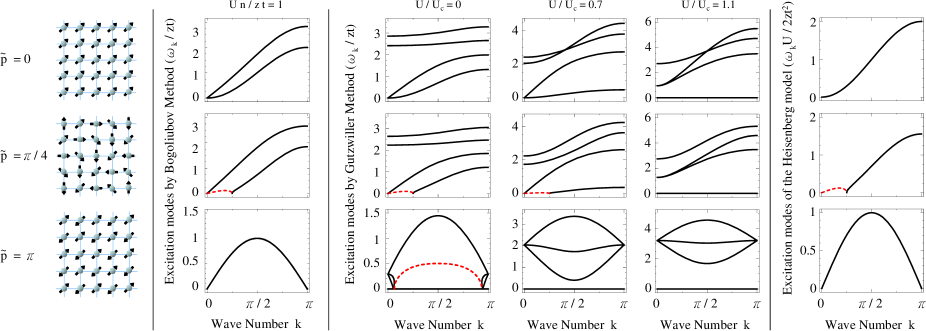
Figure 3: Dispersions of excitation modes for different spin twists along diagonal $\mathbf{p}=\tilde{p}(\hat{x}+\hat{y})$ where $\tilde{p}=0,\frac{\pi}{4}$ and $\pi$ obtained with Bogoliubov theory, Gutzwiller approach, and within Heisenberg model. Solid lines are modes with real energies while the red dashed lines are the imaginary part of complex energies, which appears in conjugate pairs but only the positive imaginary part is plotted. Note the energies of collective modes from Heisenberg model are in units of $2zt^{2}/U$ while those from Bogoliubov theory and Gutzwiller ansatz are in units of $zt$.

In the middle column of Fig. 3 we plot the dispersion of the low energy collective modes (with $\mathbf{k}\parallel\mathbf{p}$) of the ferromagnetic state, the Neel state and a spin-spiral state with a period of $4$ lattice spacings, for different interaction strengths. The ferromagnetic state has two gapless modes in the weakly interacting limit: a linearly dispersing charge mode and a quadratically dispersing spin mode. As interaction strength is increased towards the critical interaction for the superfluid-insulator transition, $U_{c}$, the charge mode dispersion is almost unaffected, while the spin mode dispersion flattens out. Beyond the critical coupling, in the Mott phase, the charge mode is gapped out while the zero energy spin mode becomes dispersionless. This is an artifact of our variational approach and we will discuss in the next section how this degeneracy can be lifted by considering the super-exchange mechanism of spin fluctuations. As soon as a spin current is imposed (say for the spin-spiral state), the spin mode develops a DI near $k=0$ in the superfluid phase. Beyond the critical coupling, the DI vanishes in the Gutzwiller approach and we recover the non-dispersing spin mode. In the weakly interacting limit, the Neel state develops a dynamical instability for collective modes around $k=\pi/2$. This dynamical instability however vanishes before the Mott transition point is reached.

Comparing the results from the Gutzwiller ansatz to those from the Bogoliubov theory, we find that for a given $\tilde{p}$, the discrepancy between the two theories increases with $U/t$, while for a given $U/t$, the discrepancy increases with increasing $\tilde{p}$. This is understood from the fact that the effective Mott boundary in presence of spin currents is given by $U=U_{c}\gamma_{p}$, and so, increasing the pitch of the spin-twist pushes the system closer to the Mott phase, where the validity of the Bogoliubov theory is suspect.

Fig. 4 is the stability phase diagram of the two component bosons in the interaction-spin-twist plane. We see that any finite spin-twist leads to DI in the weakly interacting regime, whereas, for $U>U_{c}/2$, states with $\tilde{p}$ around $\pi$ (including the Neel state) becomes stable. The color scale in the plot represents the growth rate of the most unstable fluctuation mode in the dynamically unstable region. The spin $1/2$ nature of the particles is evident in the asymmetry of the growth rate between $\tilde{p}=0$ and $\tilde{p}=2\pi$. Due to Berry’s phase effects the system is only symmetric under $4\pi$ (and not $2\pi$) twist of the spin phase.

As in the case of mass current in Sec. II, the validity of our Gutzwiller approach, and hence the results of Fig. 4, are correct only if the fluctuation occupation ($\sum_{n>0}d_{ni}^{\dagger}d_{ni}$ in Appendix B) is small. In the 2D case, we find that it is indeed small ($<0.1$) for the majority of the stable regime, but quickly goes up near the DI boundary, which is expected as a precursor of instability. The most severe case happens at the DI boundary for the Neel state, having fluctuation occupation $\sim 0.4$.

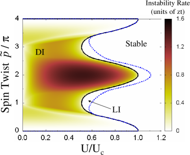
Figure 4: Phase Diagram of spin current on a lattice. This is computed with $\gamma_{\mathbf{p}}=\cos\tilde{p}$ which represents a spin current put along the diagonal of a square lattice. The shading indicates the growth rate of the most unstable mode in the dynamically unstable regime.

III.3 Heisenberg Model

It was previously shown that the two-component Bose-Hubbard model (5) reduces to a ferromagnetic spin model in the deep Mott phase Duan et al. (2003); Altman et al. (2003). Here we shall show that within the Gutzwiller ansatz, the ferromagnetic ordering is provided by the fluctuations.

First note that since a Mott phase has $\theta=0$ in our Gutzwiller ansatz, all spin twists $\mathbf{p}$ give the same variational ground state energy. The correction to the ground state energy due to fluctuations is $\Delta E=\frac{1}{2}\sum_{k}\left(-\mathrm{Tr}M+\sum_{\alpha}\omega_{\alpha k}\right)$ where $M$ is the matrix derived in Appendix B and $\omega_{\alpha k}$ are the eigenenergies. We expand $\omega_{\alpha k}$ to the first order in $1/U$ and find that the correction to the ground state energy for different spin twists obeys $E\left(\mathbf{p}\right)-E\left(0\right)=-\frac{Nt^{2}}{U}\left(\gamma_{\mathbf{p}}-1\right)$. This is exactly the energy difference due to different magnons in a ferromagnetic Heisenberg model.

However, one should be careful in interpreting the stability in the deep Mott regime. As noted previously Altman et al. (2003), we find a non-dispersing zero mode in the Mott phase, which emerges because there is no energy cost to create a spin-flip locally. We note that this is not physical and will be lifted at the next order in perturbation theory. Another way to understand this is that the product form we chose for the variational state [Eq. (12)] is unable to capture the spin ordering in the Mott phase, because charge fluctuations are completely absent. To account for this, one can rotate the state with a suitable unitary transformation $\left|G^{\prime}\right\rangle=e^{iS}\left|G\right\rangle$, which amounts to a canonical transformation $H^{\prime}=e^{-iS}He^{iS}$ on the Hamiltonian MacDonald et al. (1988); Chernyshev et al. (2004). To the lowest order, $H$ acquires the correction $-J\sum_{\left\langle ij\right\rangle}\mathbf{S}_{i}\cdot\mathbf{S}_{j}$ where $J=\frac{4t^{2}}{U}$. Using this Hamiltonian in our analysis we find that the zero mode is indeed lifted, with energy

$$\omega_{\mathbf{k}}(\mathbf{p})=\frac{zJ}{2}\sqrt{\left(\gamma_{\mathbf{p}}-\gamma_{\mathbf{k}}\right)\left(\gamma_{\mathbf{p}}-\frac{1}{2}\left(\gamma_{\mathbf{k}+\mathbf{p}}+\gamma_{\mathbf{k}-\mathbf{p}}\right)\right)}$$ (13)

which is plotted in the right column in Fig. 3. Note that this dispersion is identical to the usual spin mode in the Heisenberg model with spin twist $\mathbf{p}$. Similar to the Bogoliubov results, this spin mode has a LI for non-zero pitch and a DI for any pitch except for the ferromagnetic and Neel state. However a crucial difference is that the growth rate of the unstable modes in this case has order of magnitude $\frac{t^{2}}{U}$, which is much smaller than that of the DI we find in Fig. 4. This would imply that the deep Mott state is at least quasi-stable, in that the instability time scale could be much longer than the experimental time scale.

IV Instabilities of the Neel state

From the beginning of implementation of optical lattices, observing antiferromagnetically ordered states has been a holy grail of cold atom experiments. Although the original ideas involved looking for antiferromagnetic states with fermions, recently two component bosons have been proposed as an alternate medium to observe antiferromagnetism. In this context, there is a special interest in the observation of Neel state with a commensurate spin-ordering vector $\mathbf{p}=(\pi,\pi)$, which is notoriously hard to realize as a ground state in cold atom systems Lee et al. (2007); Ho (2008); Sørensen et al. (2010). In the deep Mott phase, this state is the highest energy state of the ferromagnetic spin model, and is expected to be stable Purcell and Pound (1951); Ramsey (1956); Sørensen et al. (2010) over relatively large time-scales, which has led to the idea that the physics of the Neel state may be accessed in systems which are carefully prepared to be stuck in this metastable state. In the opposite limit of the weakly interacting superfluid phase, analysis using the Bogoliubov approach in Sec. III.1 also demonstrates that the Neel state is dynamically stable. This naturally leads to the question: Is the Neel state stable throughout the phase diagram (i.e. for all interaction strengths)?

We use the Gutzwiller ansatz scheme to look at the stability of the Neel state in the intermediate interaction regime. The Gutzwiller approach shows that the Neel state is dynamically unstable for $0<U\lesssim 0.51$. The $U=0$ state is technically stable, but is mostly irrelevant for real experimental purposes as non-interacting bosons are pathological even in equilibrium (e.g. divergent compressibility) and need a finite interaction to form a stable superfluid. In Fig. 5, we plot the growth rate of the most unstable fluctuation mode (if any) of the Neel state, obtained via our Gutzwiller approach as a function of the interaction strength. The growth rate initially increases with the interaction strength in the weakly interacting limit reaching a peak at around $U/U_{c}\sim 0.3$. It then decreases with increasing interaction and vanishes at around $U/U_{c}\sim 0.5$. Thus Neel state physics can only be probed with dynamically generated states for $U/U_{c}\gtrsim 0.5$. We note that at $U/U_{c}=0.55$, the Gutzwiller ansatz predicts a condensate depletion of about $0.21$, which shows that the approximation, which involves a truncated Hilbert space, captures the essential physics in this regime. The Gutzwiller results in the very weakly interacting regime, $U\rightarrow 0$, are, however, suspect as the large number fluctuations in this limit are incompatible with the truncation of the Hilbert space used in the Gutzwiller scheme. In fact, to leading order in the interaction strength, the Bogoliubov theory, which predicts a stable Neel state, is much more trustworthy than the Gutzwiller scheme. It would be interesting to see how the instability rates in the Gutzwiller approximation change with increasing the size of the Hilbert space, but this much more complicated problem is beyond the scope of this paper.

Figure 5: Growth rate of the most unstable fluctuation mode of Neel state as a function of $U$, the on-site interaction, analyzed via the Gutzwiller approach. The result is expected to be invalid near $U=0$ because it is in superfluid phase.

V Conclusion

In this work we have analyzed the stability of mass and spin current carrying two-component Bose condensates in optical lattices. We have approached the problem via Bogoliubov theory and the Gutzwiller ansatz, to handle respectively the weakly interacting superfluid phase and the regime near the Mott boundary. For small spin current and small interaction the two approaches agree, but deviate when we increase the spin current or the interaction strength. In the deep Mott phase, we addressed the subtleties we encountered with our variational approach, and showed that the ferromagnetic Heisenberg model provides an adequate description in this limit.

For mass current carrying states, we find that the stability phase diagram of the two component bosons qualitatively follow that of the spinless bosons. The current carrying states are dynamically unstable beyond a critical value of the current, and the critical current monotonically decreases with increase in interaction strength, vanishing at the critical coupling for the superfluid-insulator transition. For the spin-current carrying states, we find, within Bogoliubov theory, that the system is unstable to any finite spin current in the weakly interacting limit, with the exception of the Neel state (with a spin twist of $(\pi,\pi)$. The Gutzwiller approach also predicts a similar scenario with the only difference being that the Neel state is also dynamically unstable in this regime. The Gutzwiller approach shows that the region of instability in the spin-current-interaction plane decreases with increasing interaction, with states around the Neel state (spin twist close to $(\pi,\pi)$) being the dynamically stable states. The Heisenberg model in the atomic limit also predicts dynamical instability for all current carrying states except the Neel state. Finally we stressed the fact that although the Neel state is stable in the two extreme limits of strong and weak interactions, it can develop instabilities for intermediate interaction strengths.

Although energetic instabilities would be very hard to observe experimentally in cold atom systems, the dynamical instabilities of the current carrying states should be fairly easily observable as dramatic phenomena. The typical experiment would consist of creating a spin-current carrying state by tuning a spatially varying artificial Zeeman field. Such fields with commensurate wavevectors have already been produced in the laboratories. By tuning the amplitude of these fields to a very large value, so that the Zeeman energy is the largest energy in the problem, the spin-current carrying states can be generated as the ground states of the system of bosons. Once the field is turned off, the system would exhibit violent disruption of the spin pattern if it is in a dynamically unstable state, as long as the inverse growth rate of the unstable modes are small compared to experimental timescales. Since the maximum growth rate of unstable modes is $\sim 1.5zt$, this growth dynamics should be observable over a wide range of experimental parameters. We thus hope that our predicted instabilities would be easily seen by future experiments on cold atoms.

Appendix A Analysis for Spinless Condensate

Here we shall give the details of calculations in Sec. II. The variational energy using the three-state Gutzwiller ansatz with phase twist $\mathbf{p}$ is:

$$\epsilon \equiv \frac{1}{N}\left\langle\Omega\right|H\left|\Omega\right\rangle$$ (14)

$$= \left(\frac{U}{2}+\mu\cos\chi\right)\sin^{2}\frac{\theta}{2}-\frac{tz\bar{n}}{4}\gamma_{\mathbf{p}}\sin^{2}\theta\times$$

$$\left(1+\bar{n}^{-1}\sin^{2}\frac{\chi}{2}+\sqrt{1+\bar{n}^{-1}}\sin\chi\cos 2\eta\right)$$

where $\gamma_{\mathbf{p}}=z^{-1}\sum_{\mathbf{\delta}}e^{i\mathbf{p}.\mathbf{\delta}}$, which reduces to $\gamma_{\mathbf{p}}=\frac{\cos p+(d-1)}{d}$ for a current put along an axis of a $d$-dimension cubic lattice.

Since $\left|\Omega\right\rangle$ has filling ratio $\nu=\bar{n}-\sin^{2}\frac{\theta}{2}\cos\chi$, to ensure commensurate filling one should find a $\mu$ such that the minimum of $\epsilon$ occurs at $\chi=\frac{\pi}{2}$. For convenience we consider only the limit $\bar{n}\gg 1$. Then with $\mu=0$, the minimum of $\epsilon$ is attained with $\chi=\frac{\pi}{2}$, $\eta=0$, and

$$\cos\theta=\begin{cases}u/\gamma_{\mathbf{p}},&0<u/\gamma_{\mathbf{p}}<1\\ 1,&\mathrm{otherwise}\end{cases}$$ (15)

where $u\equiv\frac{U}{4zt\bar{n}}$. One can also check that this is a stationary solution by varying $\epsilon$ locally to leading orders to find $\delta\epsilon=\frac{1}{4}\left(U-4zt\bar{n}\gamma_{\mathbf{p}}\cos\theta\right)\sin\theta\delta\theta$. The solution $\sin\theta=0$ corresponds to a Mott phase while the other solution corresponds to a superfluid state.

Performing the fluctuation expansion as outlined in the text, one finds $H=\frac{zt\bar{n}}{2}\sum_{\mathbf{k}}\Psi_{\mathbf{k}}^{\dagger}M_{\mathbf{k}}\Psi_{\mathbf{k}}$ where, in the superfluid and Mott phase, $M$ are respectively

$$M_{\mathrm{sf}} = \left(\begin{array}[]{cccc}2\gamma_{\mathbf{p}}-\cos^{2}\theta\gamma_{+}&-\cos^{2}\theta\gamma_{+}&-\cos\theta\cos\frac{\theta}{2}\gamma_{-}&\cos\theta\cos\frac{\theta}{2}\gamma_{-}\\ -\cos^{2}\theta\gamma_{+}&2\gamma_{\mathbf{p}}-\cos^{2}\theta\gamma_{+}&-\cos\theta\cos\frac{\theta}{2}\gamma_{-}&\cos\theta\cos\frac{\theta}{2}\gamma_{-}\\ -\cos\theta\cos\frac{\theta}{2}\gamma_{-}&-\cos\theta\cos\frac{\theta}{2}\gamma_{-}&\left(2\gamma_{\mathbf{p}}-\gamma_{+}\right)\cos^{2}\frac{\theta}{2}&\cos^{2}\frac{\theta}{2}\gamma_{+}\\ \cos\theta\cos\frac{\theta}{2}\gamma_{-}&\cos\theta\cos\frac{\theta}{2}\gamma_{-}&\cos^{2}\frac{\theta}{2}\gamma_{+}&\left(2\gamma_{\mathbf{p}}-\gamma_{+}\right)\cos^{2}\frac{\theta}{2}\end{array}\right)$$ (20)

$$M_{\mathrm{mott}} = \left(\begin{array}[]{cccc}2u-\gamma_{+}&-\gamma_{+}&-\gamma_{-}&\gamma_{-}\\ -\gamma_{+}&2u-\gamma_{+}&-\gamma_{-}&\gamma_{-}\\ -\gamma_{-}&-\gamma_{-}&2u-\gamma_{+}&\gamma_{+}\\ \gamma_{-}&\gamma_{-}&\gamma_{+}&2u-\gamma_{+}\end{array}\right)$$ (25)

where $\gamma_{\pm}\equiv\frac{1}{2}\left(\gamma_{\mathbf{k}+\mathbf{p}}\pm\gamma_{\mathbf{k}-\mathbf{p}}\right)$. Note that the problem reduces to the one considered before Altman and Auerbach (2002) in the limit of $\mathbf{p}=0$. The spectrum is found by diagonalizing $\sigma M$ where $\sigma\equiv\mathrm{diag}\left(1,-1,1,-1\right)$ which would give a spectrum of the form $\left\{\pm\frac{1}{2}\omega_{\alpha\mathbf{k}}\right\}$.

Appendix B Analysis for Two-Component Condensate

We take $\left|\Omega\right\rangle$ from Eq. (12) with a spin twist $\mathbf{p}$ imposed to evaluate the variational energy $\epsilon=\frac{1}{N}\left\langle\Omega\right|H\left|\Omega\right\rangle$. With some algebra it can be shown that one can first set $\theta_{1,3,4}$ to be $\pi/2$, after which

$$\epsilon = \left(\frac{U}{2}+\mu\cos\theta_{2}\right)\sin^{2}\frac{\theta}{2}-\frac{tz\sin^{2}\theta}{8}\gamma_{\mathbf{p}/2}$$ (26)

$$\times\left(3-\cos\theta_{2}+2\sqrt{2}\sin\theta_{2}\right).$$

To ensure a filling ratio $\nu=1$ one must set $\mu=-\frac{zt}{2}\gamma_{\mathbf{p}/2}\cos^{2}\frac{\theta}{2}$. Then the variational energy is minimized by $\theta_{i>0}=\frac{\pi}{2}$ and

$$\cos\theta=\begin{cases}u/\gamma_{\mathbf{p}/2}&,0<u/\gamma_{\mathbf{p}/2}<1\\ 1&,\mathrm{otherwise}\end{cases}$$ (27)

where $u\equiv\frac{U}{\left(3+2\sqrt{2}\right)zt}$. The six states are written in terms of the E: $\left|\alpha\right\rangle\rightarrow t_{\alpha}^{\dagger}\left|\mathrm{vac}\right\rangle$ satisfying the constraint $\sum_{\alpha}t_{\alpha}^{\dagger}t_{\alpha}=1$, where $\alpha$ could be the empty, 1 spin-up, 1 spin-down, 2 spin-up, 1 spin-up + 1 spin-down, or the 2 spin-down states. The boson creation/annihilation operators are replaced by the pseudospin operators:

$$b_{i\uparrow}^{\dagger} \rightarrow t_{\uparrow}^{\dagger}t_{0}+t_{\uparrow\downarrow}^{\dagger}t_{\downarrow}+\sqrt{2}t_{\uparrow\uparrow}^{\dagger}t_{\uparrow}$$ (28)

$$b_{i\downarrow}^{\dagger} \rightarrow t_{\downarrow}^{\dagger}t_{0}+t_{\uparrow\downarrow}^{\dagger}t_{\uparrow}+\sqrt{2}t_{\downarrow\downarrow}^{\dagger}t_{\downarrow}$$ (29)

The unitary transformation analogous to Eq. (4) is chosen as:

$$\left(\begin{array}[]{c}d_{0i}^{\dagger}\\ d_{1i}^{\dagger}\\ d_{2i}^{\dagger}\\ d_{3i}^{\dagger}\\ d_{4i}^{\dagger}\\ d_{5i}^{\dagger}\end{array}\right)=\left(\begin{array}[]{cccccc}\frac{1}{\sqrt{2}}\sin\frac{\theta}{2}&\frac{e^{i\mathbf{p}\cdot\mathbf{x}_{i}/2}}{\sqrt{2}}\cos\frac{\theta}{2}&\frac{e^{-i\mathbf{p}\cdot\mathbf{x}_{i}/2}}{\sqrt{2}}\cos\frac{\theta}{2}&\frac{e^{i\mathbf{p}\cdot\mathbf{x}_{i}}}{2\sqrt{2}}\sin\frac{\theta}{2}&\frac{1}{2}\sin\frac{\theta}{2}&-\frac{e^{-i\mathbf{p}\cdot\mathbf{x}_{i}}}{2\sqrt{2}}\sin\frac{\theta}{2}\\ -\frac{1}{\sqrt{2}}\cos\frac{\theta}{2}&\frac{e^{i\mathbf{p}\cdot\mathbf{x}_{i}/2}}{\sqrt{2}}\sin\frac{\theta}{2}&\frac{e^{-i\mathbf{p}\cdot\mathbf{x}_{i}/2}}{\sqrt{2}}\sin\frac{\theta}{2}&-\frac{e^{i\mathbf{p}\cdot\mathbf{x}_{i}}}{2\sqrt{2}}\cos\frac{\theta}{2}&-\frac{1}{2}\cos\frac{\theta}{2}&-\frac{e^{-i\mathbf{p}\cdot\mathbf{x}_{i}}}{2\sqrt{2}}\cos\frac{\theta}{2}\\ \frac{1}{\sqrt{2}}&0&0&-\frac{e^{i\mathbf{p}\cdot\mathbf{x}_{i}}}{2\sqrt{2}}&-\frac{1}{2}&-\frac{e^{-i\mathbf{p}\cdot\mathbf{x}_{i}}}{2\sqrt{2}}\\ 0&\frac{e^{i\mathbf{p}\cdot\mathbf{x}_{i}/2}}{\sqrt{2}}&-\frac{e^{-i\mathbf{p}\cdot\mathbf{x}_{i}/2}}{\sqrt{2}}&0&0&0\\ 0&0&0&\frac{e^{i\mathbf{p}\cdot\mathbf{x}_{i}}}{\sqrt{2}}&\frac{1}{\sqrt{2}}&\frac{e^{-i\mathbf{p}\cdot\mathbf{x}_{i}}}{\sqrt{2}}\\ 0&0&0&\frac{e^{i\mathbf{p}\cdot\mathbf{x}_{i}}}{\sqrt{2}}&0&-\frac{e^{-i\mathbf{p}\cdot\mathbf{x}_{i}}}{\sqrt{2}}\end{array}\right)\left(\begin{array}[]{c}t_{0i}^{\dagger}\\ t_{\uparrow i}^{\dagger}\\ t_{\downarrow i}^{\dagger}\\ t_{\uparrow\uparrow i}^{\dagger}\\ t_{\uparrow\downarrow i}^{\dagger}\\ t_{\downarrow\downarrow i}^{\dagger}\end{array}\right)$$ (30)

and we set both $d_{0i}$ and $d_{0i}^{\dagger}$ to be $\sqrt{1-\sum_{n>0}d_{ni}^{\dagger}d_{ni}}\approx 1-\frac{1}{2}\sum_{n>0}d_{ni}^{\dagger}d_{ni}$ because $d_{0i}^{\dagger}$ is macroscopically occupied. The validity of this expansion should be checked after the Bogoliubov transformation to ensure consistency.

Written in terms of $d_{n>0}$ and to the lowest (quadratic) order, $H=\frac{zt}{2}\sum_{\mathbf{k}}\left(\omega_{4\mathbf{k}}d_{4\mathbf{k}}^{\dagger}d_{4\mathbf{k}}+\Psi_{\mathbf{k}}^{\dagger}M\Psi_{\mathbf{k}}\right)$ where $\Psi_{\mathbf{k}}^{\dagger}\equiv\left(d_{1\mathbf{k}}^{\dagger},d_{1,-\mathbf{k}},d_{2\mathbf{k}}^{\dagger},d_{2,-\mathbf{k}},d_{3\mathbf{k}}^{\dagger},d_{3,-\mathbf{k}},d_{5\mathbf{k}}^{\dagger},d_{5,-\mathbf{k}}\right)$ and $M$ is an $8\times 8$ matrix, whose non-zero entries are:

$$M_{1,1}=M_{2,2} = \frac{1}{2}\left(3+2\sqrt{2}\right)\left(u\cos\theta+\gamma_{\mathbf{p}/2}\sin^{2}\theta\right)$$

$$-\frac{1}{8}\gamma_{+}\left(9-2\sqrt{2}+\left(3+2\sqrt{2}\right)\cos 2\theta\right)$$

$$M_{3,3}=M_{4,4} = \frac{1}{4}\left(3+2\sqrt{2}\right)\left(u+u\cos\theta+\gamma_{\mathbf{p}/2}\sin^{2}\theta\right)$$

$$-\frac{3}{2}\gamma_{+}\cos^{2}\frac{\theta}{2}$$

$$M_{5,5}=M_{6,6} = -\frac{1}{2}\left(3+2\sqrt{2}\right)(u-\gamma_{\mathbf{p}/2}(1+\cos\theta))\sin^{2}\frac{\theta}{2}$$

$$-\frac{1}{2}\gamma_{+}\sin^{2}\frac{\theta}{2}$$

$$M_{7,7}=M_{8,8} = \frac{1}{2}\cos^{2}\frac{\theta}{2}\left(\left(3+2\sqrt{2}\right)u-2\gamma_{+}\right)$$

$$+\frac{\gamma_{\mathbf{p}/2}}{2}\cos^{2}\frac{\theta}{2}\left(4+2\sqrt{2}-\left(3+2\sqrt{2}\right)\cos\theta\right)$$

$$M_{1,2}=M_{2,1} = -\frac{1}{8}\gamma_{+}\left(-3+6\sqrt{2}+\left(3+2\sqrt{2}\right)\cos 2\theta\right)$$

$$M_{3,4}=M_{4,3} = \sqrt{2}\gamma_{+}\cos^{2}\frac{\theta}{2}$$

$$M_{1,3}=M_{3,1} = M_{2,4}=M_{4,2}=\frac{1}{2}\gamma_{\mathbf{p}/2}\cos\frac{\theta}{2}-\frac{1}{2}\gamma_{+}\cos^{3}\frac{\theta}{2}$$

$$M_{1,4}=M_{4,1} = M_{2,3}=M_{3,2}=\frac{1}{2}\gamma_{+}\cos\frac{\theta}{2}\sin^{2}\frac{\theta}{2}$$

$$M_{1,5}=M_{5,1} = -M_{2,6}=-M_{6,2}$$

$$= \frac{1}{4}\gamma_{-}\left(-1+\sqrt{2}+\left(1+\sqrt{2}\right)\cos\theta\right)\sin\frac{\theta}{2}$$

$$M_{1,6}=M_{6,1} = -M_{2,5}=-M_{5,2}$$

$$= \frac{1}{4}\gamma_{-}\left(-1+\sqrt{2}-\left(1+\sqrt{2}\right)\cos\theta\right)\sin\frac{\theta}{2}$$

$$M_{1,7}=M_{7,1} = -M_{2,8}=-M_{8,2}$$

$$= \frac{1}{4}\gamma_{-}\cos\frac{\theta}{2}\left(2-\sqrt{2}+\left(2+\sqrt{2}\right)\cos\theta\right)$$

$$M_{1,8}=M_{8,1} = -M_{2,7}=-M_{7,2}$$

$$= \frac{1}{4}\gamma_{-}\cos\frac{\theta}{2}\left(2-\sqrt{2}-\left(2+\sqrt{2}\right)\cos\theta\right)$$

$$M_{3,5}=M_{5,3} = -M_{4,6}=-M_{6,4}=\frac{\gamma_{-}}{2\sqrt{2}}$$

$$M_{3,6}=M_{6,3} = -M_{4,5}=-M_{5,4}=\frac{\gamma_{-}}{4}\sin\theta$$

$$M_{3,7}=M_{7,3} = -M_{4,8}=-M_{8,4}=\gamma_{-}\cos^{2}\frac{\theta}{2}$$

$$M_{3,8}=M_{8,3} = -M_{4,7}=-M_{7,4}=\frac{\gamma_{-}}{\sqrt{2}}\cos^{2}\frac{\theta}{2}$$

$$M_{5,7}=M_{7,5} = M_{6,8}=M_{8,6}$$

$$= -\frac{1}{4}\left(2+\sqrt{2}\right)\gamma_{\mathbf{p}/2}\sin\theta-\frac{\gamma_{+}}{2\sqrt{2}}\sin\theta$$

where $\gamma_{\pm}\equiv\frac{1}{2}\left(\gamma_{\mathbf{k}+\mathbf{p}/2}\pm\gamma_{\mathbf{k}-\mathbf{p}/2}\right)$. Diagonalizing $\sigma M$ where $\sigma\equiv\mathrm{diag}\left(1,-1,1,-1,1,-1,1,-1\right)$ gives the spectrum.

References

- Morsch and Oberthaler (2006) O. Morsch and M. Oberthaler, Rev. Mod. Phys. 78, 179 (2006).
- Whitham (1965) G. Whitham, J. Fluid Mech. 22, 273 (1965).
- Benjamin and Hasselmann (1967) T. B. Benjamin and K. Hasselmann, Proc. Roy. Soc. Ser. A 299, 59 (1967).
- Ostrovskii (1964) L. A. Ostrovskii, Sov. Phys. Tech. Phys. 8, 679 (1964).
- Ostrovskii (1967) L. A. Ostrovskii, Sov. Phys. JETP 24, 797 (1967).
- Hasegawa and Brinkman (1980) A. Hasegawa and W. Brinkman, IEEE J. Quantum Electron. 16, 694 (1980).
- Tai et al. (1986) K. Tai, A. Hasegawa, and A. Tomita, Phys. Rev. Lett. 56, 135 (1986).
- Hasegawa (1972) A. Hasegawa, Phys. Fluids 15, 870 (1972).
- Pesme et al. (1988) D. Pesme, S. J. Karttunen, R. R. E. Salomaa, G. Laval, and N. Silvestre, Laser Part. Beams 6, 199 (1988).
- McKinstrie and Bingham (1989) C. McKinstrie and R. Bingham, Phys. Fluids B 1, 230 (1989).
- Jo et al. (2009) G.-B. Jo, Y.-R. Lee, J.-H. Choi, C. A. Chistensen, T. H. Kim, J. H. Thywissen, D. E. Pritchard, and W. Ketterle, Science 325, 1521 (2009).
- Pekker et al. (2011) D. Pekker, M. Babadi, R. Sensarma, N. Zinner, L. Pollet, M. W. Zwierlein, and E. Demler, Phys. Rev. Lett. 106, 050402 (2011).
- Wu and Niu (2001) B. Wu and Q. Niu, Phys. Rev. A 64, 061603 (2001).
- Konotop and Salerno (2002) V. V. Konotop and M. Salerno, Phys. Rev. A 65, 021602 (2002).
- Smerzi et al. (2002) A. Smerzi, A. Trombettoni, P. G. Kevrekidis, and A. R. Bishop, Phys. Rev. Lett. 89, 170402 (2002).
- Machholm et al. (2003) M. Machholm, C. J. Pethick, and H. Smith, Phys. Rev. A 67, 053613 (2003).
- Modugno et al. (2004) M. Modugno, C. Tozzo, and F. Dalfovo, Phys. Rev. A 70, 043625 (2004).
- Altman et al. (2005) E. Altman, A. Polkovnikov, E. Demler, B. I. Halperin, and M. D. Lukin, Phys. Rev. Lett. 95, 020402 (2005).
- Polkovnikov et al. (2005) A. Polkovnikov, E. Altman, E. Demler, B. Halperin, and M. D. Lukin, Phys. Rev. A 71, 063613 (2005).
- Raman et al. (1999) C. Raman, M. Köhl, R. Onofrio, D. S. Durfee, C. E. Kuklewicz, Z. Hadzibabic, and W. Ketterle, Phys. Rev. Lett. 83, 2502 (1999).
- Cataliotti et al. (2003) F. Cataliotti, L. Fallani, F. Ferlaino, C. Fort, P. Maddaloni, and M. Inguscio, New J. of Phys. 5, 71 (2003).
- Fallani et al. (2004) L. Fallani, L. De Sarlo, J. E. Lye, M. Modugno, R. Saers, C. Fort, and M. Inguscio, Phys. Rev. Lett. 93, 140406 (2004).
- Anker et al. (2005) T. Anker, M. Albiez, R. Gati, S. Hunsmann, B. Eiermann, A. Trombettoni, and M. K. Oberthaler, Phys. Rev. Lett. 94, 020403 (2005).
- Fertig et al. (2005) C. D. Fertig, K. M. O’Hara, J. H. Huckans, S. L. Rolston, W. D. Phillips, and J. V. Porto, Phys. Rev. Lett. 94, 120403 (2005).
- De Sarlo et al. (2005) L. De Sarlo, L. Fallani, J. E. Lye, M. Modugno, R. Saers, C. Fort, and M. Inguscio, Phys. Rev. A 72, 013603 (2005).
- Mun et al. (2007) J. Mun, P. Medley, G. K. Campbell, L. G. Marcassa, D. E. Pritchard, and W. Ketterle, Phys. Rev. Lett. 99, 150604 (2007).
- Ferris et al. (2008) A. J. Ferris, M. J. Davis, R. W. Geursen, P. B. Blakie, and A. C. Wilson, Phys. Rev. A 77, 012712 (2008).
- Law et al. (2001) C. K. Law, C. M. Chan, P. T. Leung, and M.-C. Chu, Phys. Rev. A 63, 063612 (2001).
- Kuklov and Svistunov (2003) A. B. Kuklov and B. V. Svistunov, Phys. Rev. Lett. 90, 100401 (2003).
- Takeuchi et al. (2010) H. Takeuchi, S. Ishino, and M. Tsubota, Phys. Rev. Lett. 105, 205301 (2010).
- Hoefer et al. (2010) M. Hoefer, C. Hamner, J. Chang, and P. Engels, Arxiv preprint arXiv:1007.4947 (2010).
- Hamner et al. (2011) C. Hamner, J. J. Chang, P. Engels, and M. A. Hoefer, Phys. Rev. Lett. 106, 065302 (2011).
- Vengalattore et al. (2008) M. Vengalattore, S. R. Leslie, J. Guzman, , and D. M. Stamper-Kurn, Phys. Rev. Lett. 100, 170403 (2008).
- Cherng et al. (2008) R. W. Cherng, V. Gritsev, D. M. Stamper-Kurn, and E. Demler, Phys. Rev. Lett. 100, 180404 (2008).
- Sørensen et al. (2010) A. S. Sørensen, E. Altman, M. Gullans, J. V. Porto, M. D. Lukin, and E. Demler, Phys. Rev. A 81, 061603 (2010).
- Altman and Auerbach (2002) E. Altman and A. Auerbach, Phys. Rev. Lett. 89, 250404 (2002).
- Holstein and Primakoff (1940) T. Holstein and H. Primakoff, Phys. Rev. 58, 1098 (1940).
- Duan et al. (2003) L.-M. Duan, E. Demler, and M. D. Lukin, Phys. Rev. Lett. 91, 090402 (2003).
- Altman et al. (2003) E. Altman, W. Hofstetter, E. Demler, and M. Lukin, New J. of Phys. 5, 113 (2003).
- MacDonald et al. (1988) A. H. MacDonald, S. M. Girvin, and D. Yoshioka, Phys. Rev. B 37, 9753 (1988).
- Chernyshev et al. (2004) A. L. Chernyshev, D. Galanakis, P. Phillips, A. V. Rozhkov, and A.-M. S. Tremblay, Phys. Rev. B 70, 235111 (2004).
- Lee et al. (2007) P. J. Lee, M. Anderlini, B. L. Brown, J. Sebby-Strabley, W. D. Phillips, and J. V. Porto, Phys. Rev. Lett. 99, 020402 (2007).
- Ho (2008) T. L. Ho, Arxiv preprint arXiv:0808.2677 (2008).
- Purcell and Pound (1951) E. M. Purcell and R. V. Pound, Phys. Rev. 81, 279 (1951).
- Ramsey (1956) N. F. Ramsey, Phys. Rev. 103, 20 (1956).