Search on the Brink of Chaos

Abstract.

The Linear Search Problem is studied from the view point of Hamiltonian dynamics. For the specific, yet representative case of exponentially distributed position of the hidden object, it is shown that the optimal orbit follows an unstable separatrix in the associated Hamiltonian system.

1. Introduction

The Linear Search Problem has a venerable history, going back to R. Bellman (’63) and A. Beck (’64). They looked into the following question:

An object is placed at a point H on the real line, according to a known probability distribution. A search plan (or trajectory) is a sequence $\textbf{{x}}=\{x_{i}\}_{i=1}^{\infty}$ with $\ldots-x_{4}<-x_{2}<0<x_{1}<x_{3}<\ldots$ (or $\ldots-x_{3}<-x_{1}<0<x_{2}<x_{4}<\ldots$). A search is performed by a searcher walking alternating to the points of the search plan, starting at $0$, until the point H is found.

The total distance traveled till the point is found is $L(\textbf{{x}},\textbf{{H}})$, and the cost of the search plan x is given by

$$E(\textbf{{x}})={\mathbb{E}}\,[L(\textbf{{x}},\textbf{{H}})].$$

The task is to find the plan x minimizing $E(\textbf{{x}})$. We are therefore in the average case analysis situation.

The search problem has been also studied in theoretical computer science, see e.g. [14], where it was called cow-path problem. There have been many interesting generalizations such as search on rays, rendezvous, search with turn cost etc. [8, 10, 1]. Finally, there is some recent work in connection with robotics, see e.g. [13].

1.1. Background on Linear Search Problem

This Linear Search Problem was studied mostly by Anatole Beck and his coauthors in a series of papers where they analyzed to great details the archetypal case of normally distributed H (see [11, 7, 9, 2, 12]). It turned out that the candidates for optimal trajectories form a 1-parametric family (parameterized by the length of the first excursion $|x_{1}|$). Using careful analysis Beck further reduced the choice of the candidates to just two initial points, of which one turned out to be the best by numerics. On the nature of these initial points, [7] stated:

…we opine that this is a question whose answer will not shed much mathematical light.

This note aims at uncovering the underlying geometric structure of the Linear Search Problem. Specifically, we argue that the correct framework here is that of Hamiltonian dynamics, especially where hyperbolicity of the underlying dynamics can be deployed. In our geometric picture the mysterious two points naturally appear at the intersection of a separatrix (that is present in the associated Hamiltonian system) with the curve of initial turning points.

To this end we analyze in detail a one-sided version of the Linear Search Problem which we describe next. The original problem considered by Beck is addressed from the same viewpoint in the appendix.

We restrict our proofs mostly to the exponentially distributed position H: this is done primarily to keep the presentation succinct and clear. In the appendix we demonstrate that our approach with small modifications works for some other distribution, e.g. for one-sided Gaussian. We believe that even more general classes of distributions can be also analyzed - this will be done in a follow-up paper.

1.2. Half-line problem

We concentrate here on a one-sided gatherer version of the search problem. Here, the hiding object H is located on the half-line $\mathbb{R}_{+}$, according to some (known) probability distribution. One searches for H according to the plan

$$\textbf{{x}}=\{0=x_{0}<x_{1}<x_{2}<\ldots<x_{k}<\ldots\},$$

and stops after the step $n=n(\textbf{{x}},\textbf{{H}})$ iff the point $\textbf{{H}}\in(x_{n-1},x_{n}]$. One can think of a gatherer who mindlessly collects anything on the way, bringing the loot to the origin, where the results are analyzed (in a contrast to the searcher, who stops as soon as the sought after object is found).

As in the original version, one needs to minimize the average cost of the search, which in our case is given by

$$E(\textbf{{x}})={\mathbb{E}}[L(\textbf{{x}},\textbf{{H}})]={\mathbb{E}}\left[\sum_{k=1}^{n(\textbf{{x}},\textbf{{H}})}x_{k}\right].$$ (1)

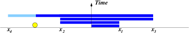
Figure 1. Linear Search Problem: two-sided searcher on the left, one-sided gatherer on the right. The cost of the indicated plans given the positions of the hidden objects are shown by darker shade.

1.3. Motivation

One-sided linear search appears naturally in quite a few applications. The initial motivation was the problem of search in unstructured Peer-to-Peer storage systems, analyzed in [4], where the relevance of Hamiltonian dynamics was first noticed. In such an unstructured network, one is sequentially flooding some (hop-)vicinity of a node, see Figure 2, with request for an item, setting the Time-to-Live at some limit, until the item is found. The cost of a plan is the total number of queries at all nodes of the network, representing the per query overhead.

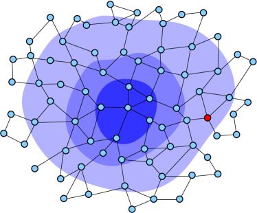
Figure 2. Search for an object in Peer-to-Peer unstructured network. The object is found after the 3rd flooding.

Further applications include robotic search, where one deals with programming a robot of low sensing and computational capabilities, unable to recognize the objects it collects. Also the problem of efficient eradication of unwanted phenomena (say irradiation of a tumor) can be mapped onto our model.

1.4. Outline of the results

We start with the general discussion of the one-sided search problem, showing in particular that the natural necessary condition of optimality implies that the optimal plan should satisfy a three-term recurrence, the variational recursion (a discrete analogue of the Euler-Lagrange equations). This reduces the dimension of phase space, but also introduces Hamiltonian dynamics.

We analyze in details a “self-similar” case of homogeneous tail distribution function, also called a Pareto distribution, and see that the phase space is split naturally into a chaotic and monotonicity regions, divided by a separatrix.

Hamiltonian dynamics associated to the variational recursion is then studied. We set up the stage for a general distribution, but mostly constrain our proofs to the case of the exponentially distributed position H of the object, i.e. to the case of

$$f(x):={\mathbb{P}}(\textbf{{H}}>x)=\exp(-x).$$

We prove that the optimal trajectories should start at the separatrix. On the other hand, the plans satisfying variational recursion are represented by a one-dimensional curve. The intersection of the separatrix with the curve gives two candidates for the starting position, mirroring the situation in the original setting of Beck et al’s papers. We conclude with several open questions.

Occasionally, we use several standard notions from the theory of dynamical systems; for definitions we refer to [15].

2. Basic properties

2.1. Basic notions

The input into the search algorithm is a plan, or a trajectory

$$\textbf{{x}}=\{x_{0}=0,x_{1},\ldots\,x_{k},\ldots\},x_{k}\geq 0,x_{k}\rightarrow\infty,$$

that is an unbounded sequence of turning points. Below we list some simple properties of the cost functional (1):

Proposition 1.

The cost of a plan is given by

$$E(\textbf{{x}})=\sum_{k=1}^{\infty}x_{k}\,{\mathbb{P}}(\textbf{{H}}>x_{k-1})=\sum_{k=1}^{\infty}x_{k}f(x_{k-1}).$$ (2)

Any optimal search plan is strictly monotone. In other words, if a plan $\textbf{{x}}=\{x_{n}\}$ is not strictly increasing, there is a naturally modified strictly monotone plan $\tilde{\textbf{{x}}}=\{\tilde{x}_{n}\}$ such that $E(\tilde{\textbf{{x}}})<E(\textbf{{x}})$.

Proof.

The contribution to the average cost is the length of excursion times the probability that such excursion will have to occur:

$$E(\textbf{{x}},\textbf{{H}})=\sum_{k}x_{k}\cdot{\mathbf{1}}(\textbf{{H}}>x_{k-1})$$

which implies (2).

Now, assume that a plan ${\bf x}$ is not strictly monotone. Consider a modified plan $\tilde{\textbf{{x}}}$, where the turning points preventing strict monotonicity are removed. Then, as can be verified by straightforward estimates, $E(\tilde{\textbf{{x}}})<E(\textbf{{x}})$. ∎

Proposition 2.

If the position of the object is known, then the cost of its recovery, $L:={\mathbb{E}}[\textbf{{H}}]$, is a lower bound on the cost of any trajectory

$$E({\bf x})\geq L.$$

There exists a plan of cost at most $4L+\epsilon$ (thus finite if $L$ is).

Proof.

First, note that the sum

$$E({\bf x})=\sum_{k=0}^{\infty}x_{k+1}f(x_{k})$$

is bounded below by the integral

$$\int_{0}^{\infty}f(x)dx=L.$$

Next, observe that

$$L={\mathbb{E}}[\textbf{{H}}]=-\int_{0}^{\infty}x\cdot f^{\prime}(x)dx=\int_{0}^{\infty}f(x)dx,$$

by definition and using integration by parts once.

Then, using monotonicity of $f$ we estimate this integral from below

$$L=\int_{0}^{\infty}f(x)dx=\sum_{k=0}^{\infty}\int_{x_{k}}^{x_{k+1}}f(x)dx\geq\sum_{k=0}^{\infty}(x_{k+1}-x_{k})f(x_{k+1}).$$

Evaluating the expression on the right over the geometric sequence $x_{0}=0,x_{k}=A\cdot 2^{k-1}$ $(k=1,2,\ldots)$, we have

$$L\geq\frac{1}{4}\sum_{k=0}^{\infty}f(x_{k+1})x_{k+2}.$$

Adding $x_{1}=A$ to both sides, we obtain

$$4L+A\geq E({\bf x}),$$

which proves the claim since $A$ can be taken arbitrarily small. ∎

If the tail distribution function is continuously differentiable (or even Lipshitz) on $[0,\infty)$, then the optimal trajectory does exist. In particular, one need not consider bi-infinite trajectories $\{0<\ldots<x_{-2}<x_{-1}<x_{1}<x_{2}<\ldots\}$. This is an extension of the corresponding result for the two-sided search, see e.g. [6]. However, for completeness, we give an independent proof in the next section. The Lipshitz property is essential, as was also observed by Beck and Franck, since one can construct an example for which no sequence with finitely many terms near zero is optimal. In other words, there is no first turning point, see example in the next section.

2.2. Variational recursion

Optimality of a sequence implies a local condition.

Proposition 3.

Assume the tail distribution function $f(x)={\mathbb{P}}(\textbf{{H}}>x)$ is differentiable. If the plan x is optimal, then the terms $\{x_{k}\}$ satisfy the variational recursion:

$$f(x_{n-1})+x_{n+1}f^{\prime}(x_{n})=0.$$ (3)

Proof.

It is immediate, if one notices that the cost depends on $x_{k}$ via only two terms, $f(x_{k-1})x_{k}$ and $f(x_{k})x_{k+1}$. ∎

This allows us to find $x_{n+1}$ as a function of $x_{n-1},x_{n}$,

$$x_{n+1}=-\frac{f(x_{n-1})}{f^{\prime}(x_{n})}$$

and to reconstruct the whole optimal plan from its first two points, $x_{0}=0$ and $x_{1}$.

In fact, it is useful to think of $\{x_{k}\}_{k=0,1,\ldots}$ as of iterations of the mapping ${\mathbf{R}}:\mathbb{R}_{+}^{2}\to\mathbb{R}_{+}^{2}$ given by

$${\mathbf{R}}:(x,y)\mapsto(y,-f(x)/f^{\prime}(y))$$

(which we will still be referring to as variational recursion).

3. Existence of an optimal sequence

For the two-sided (Beck-Bellman) search problem, the existence of the optimal search plans was shown in [11, 6] and some improvements appeared in the subsequent papers. For completeness, we supply the existence proof for the one-sided case, as we consider in detail the associated nonlinear map.

Recall the cost functional

$$E({\bf x})=\sum_{k=0}^{\infty}x_{k+1}f(x_{k})$$

and formulate the minimization problem:

$$\hskip 28.45274ptE_{0}={\rm inf}\left\{E({\bf x}),{\bf x}=(\ldots,x_{-2},x_{-1},x_{0},x_{1},x_{2},...,x_{k},...),x_{j}>0,j\in{\mathbb{N}},x_{k}\rightarrow\infty\right\}.$$ (4)

Note that we do not restrict the sequence to have the first term. We will prove this. On the other hand, if $f(x)$ does not vanish for any $x\geq 0$ there can be no other density points for an optimal plan, for otherwise the cost would be infinite.

Clearly, $E_{0}\geq 0$, since $E\geq 0$. By definition of the infimum, there exists a minimizing sequence $\{{\bf x}^{(n)}\}$ such that

$$E({\bf x}^{(n)})\rightarrow E_{0}.$$

The goal is to show that there is a convergent subsequence such that ${\bf x}^{(n_{k})}\rightarrow{\bf x}^{*}$ and $E({\bf x}^{(n_{k})})\rightarrow E_{0}.$

Proposition 4 (Properties of minimizing sequences).

Assume $f$ is Lipshitz and $f(x)\neq 0$ for any $x\geq 0$. In the minimization problem (4), there exist two positive monotone sequences, $\{a_{k}\}_{k=0}^{\infty},\{b_{k}\}_{k=0}^{\infty}$, such that $a_{k}<b_{k}$, $a_{k}\rightarrow\infty$, $b_{k}\rightarrow\infty$ and there is a minimizing subsequence $\{\textbf{{x}}^{(n)}\}$ such that $a_{k}<x_{k}^{(n)}<b_{k}$.

Proof.

First, we note that $E_{0}\leq 4L$ is a bounded quantity, see the previous section. To prove existence of $\{b_{k}\}$, we first observe that any minimizing sequence must satisfy $E({\bf x}^{(n)})\leq 2E_{0}$, for sufficiently large $n$. Thus, $x_{1}\leq 2E_{0}=b_{1}$ and then $x_{2}f(x_{1})\leq 2E_{0}$. Therefore,

$$x_{2}\leq\frac{2E_{0}}{f(x_{1})}\leq\frac{2E_{0}}{f(2E_{0})}.$$

We define then $b_{2}=2E_{0}/f(2E_{0})$. Proceeding by induction,

$$b_{k+1}=2E_{0}/f(b_{k}(E_{0})),$$ (5)

we obtain the desired sequence. Note that the sequence is strictly monotone as

$$xf(x)<L\leq E_{0}<2E_{0},$$

and therefore, the mapping (5) cannot a fixed point $x=2E_{0}/f(x)$.

Thus, the sequence $\{b_{k}\}$ monotonically grows to infinity and it bounds the corresponding terms of the minimizing sequence.

To establish lower bounding sequence we prove

Lemma 1.

Assume $f$ is Lipshitz and let ${\bf x}$ be a monotone, possibly bi-infinite, sequence of turning points. Assume $x_{m}<1/2C_{L}$, then the modified sequence $\tilde{\textbf{{x}}}$ with all $x_{j}(j<m)$ removed, will have lower cost.

Proof.

Rewrite

$$E(\textbf{{x}})=\sum_{k}x_{k+1}f(x_{k})=\ldots+x_{m-1}f(x_{m-2})+x_{m}f(x_{m-1})+x_{m+1}f(x_{m})+\ldots$$

and the modified sequence

$$E(\tilde{\textbf{{x}}})=x_{m}+x_{m+1}f(x_{m})+\ldots.$$

We need to show

$$x_{m}<\ldots+x_{m-1}f(x_{m-2})+x_{m}f(x_{m-1}).$$

Rearranging some terms we get,

$$\frac{1-f(x_{m-1})}{x_{m-1}}<\ldots+\frac{f(x_{m-2})}{x_{m}}.$$

The left handside is bounded by the Lipshitz constant $C_{L}$ and the right handside is bounded from below by $1/x_{m}-C_{L}$. Therefore, by choosing $x_{m}<1/2C_{L}$, we obtain the desired result. ∎

Therefore, an optimal sequence of turning points is one-sided and there is at most one point in the interval $[0,\delta=1/2C_{L}]$. Then, we let $a_{0}=0$ and $a_{1}=\delta$.

Now, the sequence $\{a_{k}\}$ can be constructed using monotonicity $a_{k+1}\geq a_{k}$ and that there are finitely many terms on any interval of, say, unit size: $|\delta,\delta+1|,|\delta+1,\delta+2|$, etc.

Monotonicity has been proved in the previous section by showing that in nonmonotone sequence, by deleting the appropriate terms, we obtain a strictly monotone sequence with smaller cost.

∎

Theorem 1.

There exists a converging subsequence, ${\bf x}^{(n)}\rightarrow{\bf x}^{(*)}$, where ${\bf x}^{(*)}$ is strictly monotone and $x^{(*)}_{k}\rightarrow\infty$. The cost function converges $E({\bf x}^{(n)})\rightarrow E({\bf x}^{*})=E_{0}$.

Proof.

Fix $N>0$ and let ${\mathbb{P}}_{N}\textbf{{x}}=(x_{1},x_{2},...,x_{N})$. For the minimizing sequence $\textbf{{x}}^{(n)}$, let $\textbf{{x}}^{(n_{1})}$ be a subsequence for which $x^{n_{1}}_{1}\rightarrow x_{1}^{*}$. Take a subsequence of this subsequence, so that ${\mathbb{P}}_{2}{\bf x}^{(n_{2})}\rightarrow\{x_{1}^{*},x_{2}^{*}\}$. Proceeding further and using diagonal subsequence ${\bf x}^{(n_{k}),k}$, we obtain a convergent subsequence, which we will still denote by ${\bf x}^{(n)}\rightarrow{\bf x}^{*}$. The limit $\textbf{{x}}^{*}$ is a monotone sequence by construction. It must be also strictly monotone, for if not, i.e. if some terms are equal, we already know from the previous section that by removing repeated terms the cost is decreased, which contradicts the sequence being minimizing.

Now, to prove the second part of the theorem, let $E^{N}({\bf x})$ denote $N-th$ partial sum. Fix $N>0$ to be sufficiently large, and observe that $E^{N}({\bf x}^{(n)})\rightarrow E^{N}({\bf x}^{*})$ just by continuity. Because of the lower bounding sequence $\{a_{k}\}$, we can take $N$ so large that $x^{(n)}_{N}$ and $x_{N}^{*}$ are larger than any fixed number. Consider now the remainders

$$E({\bf x}^{(n)})-E^{N}({\bf x}^{(n)}),\,\,\,\,E({\bf x}^{*})-E^{N}({\bf x}^{*}),$$

which are arbitrarily small. Indeed,

$$E({\bf x})-E^{N}({\bf x})=x_{N+1}f(x_{N})+x_{N+2}f(x_{N+1})+\ldots$$

and since the sequence is minimizing we can estimate the reminder by choosing, e.g. $x_{N+k}=2^{k+1}x_{N-1}$. Next, using an argument similar to the one used in Proposition 2, we obtain the bound

$$E({\bf x})-E^{N}({\bf x})\leq 4\int_{x_{N-1}}^{\infty}f(x)dx.$$

The same bound holds for the other reminder. Thus, taking $x_{N-1}$ large enough we can assure the reminders to be arbitrarily small. This implies the convergence $E({\bf x}^{(n)})\rightarrow E({\bf x}^{*})=E_{0}$. ∎

Next we demonstrate that the Lipshitz condition is necessary. Indeed, without it we can construct an example with no initial turning point:

Example with singularity. If the tail distribution function is not Lipshitz then the sequence may fail to have the first turning point. Here, we present a simple example of one-sided search.

Let $f(x)=1-\sqrt{x}$ and assume the search is done on the unit interval $[0,1]$. It is also possible to modify this example to the infinite ray $(0,\infty)$ by changing $f(x)$ outside of any neighborhood of $0$ so it does not vanish anywhere.

Suppose, the optimal sequence is given by a one-sided sequence $\{0<x_{1}<x_{2}<x_{3}<\ldots\}$ with the cost

$$E({\bf x})=x_{1}+x_{2}(1-\sqrt{x_{1}})+x_{3}(1-\sqrt{x_{2}})+\ldots.$$

Let us insert another point $x_{0}:0<x_{0}<x_{1}$, then the cost of modified sequence is given by

$$E({\bf\tilde{x}})=x_{0}+x_{1}(1-\sqrt{x_{0}})+x_{2}(1-\sqrt{x_{1}})+\ldots.$$

Comparing them, we find that the cost of modified sequence is lower if and only if

$$x_{0}+x_{1}(1-\sqrt{x_{0}})<x_{1}\Leftrightarrow\sqrt{x_{0}}<x_{1}\Leftrightarrow x_{0}<x_{1}^{2}.$$

The latter inequality can be always achieved. Therefore, the optimal sequence does not have an initial turning point.

4. Pareto distribution

In this section we present an explicit example which illustrates our general approach: the optimal plan of the search problem belongs to an invariant manifold (separatrix) of the associated Hamiltonian map.

4.1. Cost functional

Consider a Pareto type tail distribution (analogous to that of [14])

$$f(x) = x^{-\alpha}\,\,\,{\rm if}\,\,\ x\geq 1,$$

$$f(x) = 1\,\,\,\,\,\,\,\,\,\,\,{\rm if}\,\,\ 0<x<1,$$

where we assume that $\alpha>1$ in order to have a bounded expected value.

We will use the notation, exceptionally, $x_{0}=1$, which makes formulas look simpler. Note that $x_{0}=1$ does not correspond to an actual turning point. The expected cost is given by

$$E({\bf x})=x_{1}+f(x_{1})x_{2}+f(x_{2})x_{3}+...=\sum_{n=0}^{\infty}\frac{x_{n+1}}{x_{n}^{\alpha}}.$$

The variational recursion reads in this case

$$x_{k+1}=\frac{1}{\alpha}\frac{x_{k}^{\alpha+1}}{x_{k-1}^{\alpha}}$$

or equivalently

$$\frac{x_{k+1}}{x_{k}^{\alpha}}=\frac{1}{\alpha}\frac{x_{k}}{x_{k-1}^{\alpha}}=\frac{1}{\alpha^{k}}\frac{x_{1}}{x_{0}^{\alpha}}=\frac{1}{\alpha^{k}}x_{1}.$$

Therefore, for the sequences generated by the variational recursion, with $x_{1}=x$, we can immediately compute the cost

$$E(\textbf{{x}})=\sum_{n=0}^{\infty}\alpha^{-n}x_{1}=x_{1}\frac{\alpha}{\alpha-1},$$

as a function of the initial condition $x_{1}=x$.

This expression indicates that $x_{1}$ should be as small as possible, provided the sequence satisfies the constraints of monotonicity and unbounded growth.

From the sequence definition, we have

$$\frac{x_{k+1}}{x_{k}}=\frac{1}{\alpha}\left(\frac{x_{k}}{x_{k-1}}\right)^{\alpha}$$

or denoting the ratios by $r_{k}=x_{k}/x_{k-1}$,

$$r_{k+1}=\alpha^{-1}r_{k}^{\alpha},\,\,\,r_{1}=x_{1}.$$

Defining $w_{k}=r_{k}\alpha^{-\frac{1}{\alpha-1}}$ gives

$$w_{k+1}=w_{k}^{\alpha}.$$

We clearly need to take $w_{1}\geq 1$, so that the ratios would not go to zero and the sequence $x_{k}$ would be monotone. However, since we need $x_{1}$ to be as small as possible, we take $w_{1}=1$, resulting in $x_{1}=r_{1}=\alpha^{\frac{1}{\alpha-1}}$. Therefore, the minimal cost is given by

$$E_{0}=\frac{\alpha\cdot\alpha^{\frac{1}{\alpha-1}}}{\alpha-1}=\frac{\alpha^{\frac{\alpha}{\alpha-1}}}{\alpha-1},$$ (6)

and the optimal sequence is given by

$$x_{k}=\alpha^{\frac{k}{\alpha-1}}.$$

In a particular case of $\alpha=2$, the optimal sequence is given by geometric series $x_{k}=2^{k}$.

4.2. Hamiltonian dynamics

The global structure of the dynamics defined by the variational recurrence in this homogeneous problem is shown on the Figure 3. Here we draw the invariant curves for the trajectories defined by ${\mathbf{R}}$: the iterations of a point $(x_{k},x_{k+1})$ found on one of these curves, stays on it forever. The red (thick) line corresponds to the optimal trajectory.

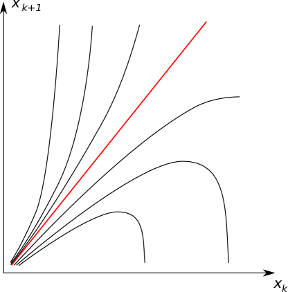
Figure 3. Phase portrait for the variational recursion for the homogeneous distribution. There are two regions: above the line $x_{k+1}=\alpha^{1/(\alpha-1)}x_{k}$, where all the orbits monotonically grow and below, where all the orbits lose monotonicity eventually.

The qualitative dynamics in this case can be summarized as follows:

• There is a region of initial values $x_{1}$ where the variational recursion stops making sense: the iterates become non-monotone. We will call this region chaotic.

• The optimal initial value is on the boundary of the chaotic set.

• The growth of the optimal plan (exponential) is far slower than the growth for generic initial values outside the chaotic region (where it is super-exponential).

The sequences can be represented as solutions of the two dimensional nonlinear map

$$x_{k+1} =r_{k+1}x_{k}$$

$$r_{k+1} =\frac{1}{\alpha}r_{k}^{\alpha}.$$

The ray $r=r^{*}=\alpha^{\frac{1}{\alpha-1}}$ is invariant. Above this ray $r=r^{*}$, the orbits go rapidly to infinity. The orbits below $r=r^{*}$ are not monotone, because $r_{k}$ monotonically decreases to zero and while $x_{k}$ may grow at first but after $r_{k}$ becomes less than 1, $x_{k}$ will be decreasing.

5. Exponential tail distribution

In this section we analyze in detail the prototypical case of exponential distribution. While, this case is sufficiently simple to allow complete understanding, the Hamiltonian dynamics is no longer integrable. Therefore, the methods that we develop would apply to other cases of interest.

5.1. Variational recursion

We consider now several key properties of the variational recursion ${\mathbf{R}}:(x,y)\mapsto(y,-f(x)/f^{\prime}(y))$.

One of the basic observation is that it preserves an area form:

Proposition 5.

The mapping ${\mathbf{R}}$ preserves the area form $\omega=f^{\prime}(x)dx\wedge dy$.

This is a rather general fact: for any recursion obtained by extremization of the functional

$$E(\textbf{{x}})=\sum_{k=0}^{\infty}F(x_{k},x_{k+1}),$$

the 2-form $\frac{\partial^{2}F}{\partial x\partial y}dx\wedge dy$ is invariant with respect to the associated two-dimensional mapping.

It is possible to explicitly give the coordinates in which the variational recursion ${\mathbf{R}}$ is Hamiltonian: if we use $(s,y)$, where $s=f(x)$ in lieu of $(x,y)$, then

$${\mathbf{R}}:(s,y)\mapsto(f(y),-s/f^{\prime}(y));$$

it maps $[0,1]\times\mathbb{R}_{+}$ into itself and preserves the Lebesgue area $ds\wedge dy$. We will be referring to these coordinate system as standard.

In the standard coordinates, the variational recursion for the exponentially distributed H (i.e. for $f(x)=\exp(-x)$) is given by

$${\mathbf{R}}:(s,y)\mapsto(e^{-y},se^{y}).$$

Further, one can see that ${\mathbf{R}}$ has a unique stationary point, $s=e^{-1},y=1$. One can verify that this fixed point is elliptic.

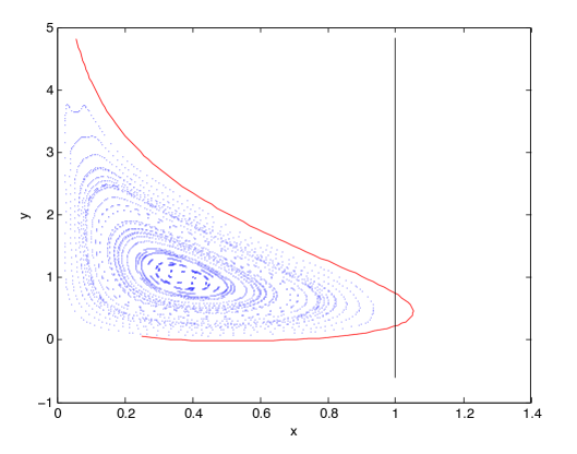
Figure 4. Several orbits of the variational recursion for exponential distribution. The solid curve separates chaotic region from the monotonicity region. The region of interest is located to the left of the vertical line $x=1$. The monotone orbits outside of the chaotic region are not present as they are rapidly mapped to infinity.

5.2. Cost functional and cost function

We already know that the optimal plan can be found only among the trajectories satisfying the variational recursion. We will set $x_{0}=0$; under this assumption the trajectories (not necessarily increasing) satisfying the variational recursion are parameterized by the first non-zero term $x_{1}:=x$. We will be denoting the corresponding family of trajectories as $\textbf{{x}}_{\mathbf{R}}(x)=\{x_{0}=0,x_{1}=x,x_{2}=x_{2}(x),\ldots\}$. For the exponentially distributed H, the first few terms of the family $\textbf{{x}}_{\mathbf{R}}(x)$ are given by $x_{1}=x;x_{2}=e^{x};x_{3}=e^{e^{x}-x}$ and so on.

Notation: We will use the term cost functional for (2), defined on the space of all trajectories x, while reserving the term cost function for the restriction of the functional $E$ to the one-parametric curve $\textbf{{x}}_{\mathbf{R}}(x)$ of solutions to variational recursion, denoting the cost function by $E(x):=E(\textbf{{x}}_{\mathbf{R}}(x))$.

For exponentially distributed H, the cost function is finite on monotonic trajectories. Indeed, in this case, unless growing without bound, the trajectory should converge to the only fixed point of the variational recursion, which is impossible as it is an elliptic point. If for some $K$, $x_{K}>1$, then for $k>K$,

$$x_{k+1}-x_{k}=\ln{x_{k+2}}\geq\ln{x_{K}}>0,$$

and $x_{k}$ grows at least as an arithmetic progression, implying the convergence of

$$E(\textbf{{x}})=\sum_{k=0}^{\infty}x_{k+1}\exp(-x_{k})=\sum_{k=0}^{\infty}\exp(-x_{k-1}).$$

Now, as the cost function $E(x)$ is a function of one variable, and we established that the optimal trajectory should be one of the family $\textbf{{x}}_{\mathbf{R}}(x)$, it might appear that the rest is straightforward: to find the minimum of $E(x)$ over the starting point $x_{1}=x$. However, if we take the formal derivative

$$\frac{dE}{dx}=\sum_{k=0}^{\infty}\frac{d}{dx}\left(x_{k+1}(x)f(x_{k}(x)\right),$$

we will see that all the terms vanish, identically (precisely because $\textbf{{x}}_{\mathbf{R}}(x)=\{x_{1}(x),x_{2}(x),\ldots\}$ satisfies the variational recursion). It might appear that $E(x)$ should be a constant! However, we already computed $E(x)$ in an example in section 4, and know that this is not the case.

The reason for this calamity is, of course, the fallacious differentiation of an infinite sum of differentiable functions with wildly growing $C^{1}$ norms.

However, if we consider the approximants

$$E^{K}(x)=\sum_{k=0}^{K}x_{k+1}f(x_{k}),$$

they can be differentiated term by term, yielding

$$\frac{dE^{K}}{dx}(x)=x_{K+1}(x)f(x_{K}(x))$$ (7)

(by telescoping).

As $E^{K}(x)$ approximates $E(x)$ to within $4E_{0}\,f(x_{K})$, which uniformly converges to zero, the existence of a local minimum of $E(x)$ in an interval where $E$ is finite would imply that the approximants $E^{K}(x)$ have local minima in that interval, for all large enough $K$. Later we will use this observation to prove that the reduced cost function has optimal solution on the separatrix.

6. Hamiltonian dynamics

Denote by ${\mathcal{P}}=\{1\geq s\geq 0,y\geq 0\}$ the phase space (in standard coordinates) on which the variational recursion acts.

6.1. Chaotic and monotone regions

Definition 1.

The region ${\mathcal{M}}_{k}$ of $k$-step monotonicity is defined as collection of points in ${\mathcal{P}}$ such that $k$-fold application of the ${\mathbf{R}}$ produces a monotonic (along $y$ coordinate) sequence. The intersection of all ${\mathcal{M}}_{k}$ is denoted by ${\mathcal{M}}_{\infty}:=\cap_{k}{\mathcal{M}}_{k}$ and is called the region of monotonicity. Its complement is called the chaotic region.

The boundary ${\mathcal{S}}$ of the monotonicity region is called the separatrix. It is not immediate that the separatrix is a curve: the monotone and chaotic regions can have rather wild structure. However, we will see that the separatrix is indeed a smooth curve, and the relevant part of it can be represented as a graph of a function in some appropriate coordinates.

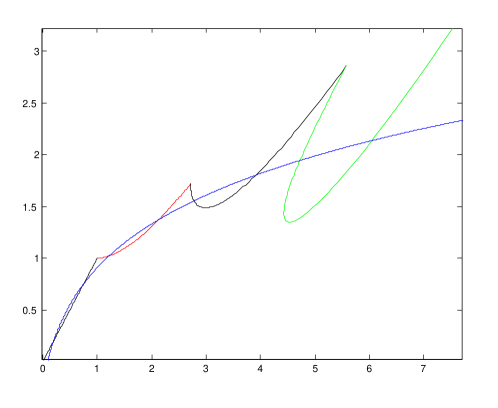
Figure 5. Invariant curve and iterated initial data in the exponential case in $(y,z)$ coordinates. The long curve is the separatrix. It corresponds to the solid curve in Figure 4. The line segment with the end points $(0,0)$ and $(1,1)$ represents a one parameter family of the initial turning points $x_{1}$. Note that the segment intersects the separatrix at exactly two points. These two points are the candidates for the optimal search sequence. The other curves are obtained by iterating the initial segment by the forward map.

6.2. Existence of separatrix: exponential distribution

The existence of the separatrix in the phase space for the exponentially distributed H is proved by applying the standard Banach contraction mapping principle.

We start by introducing more convenient coordinates in the phase space $(x,y)\rightarrow(y,z=y-x)$. Thus, $z_{k+1}=x_{k+1}-x_{k}$ “measures” monotonicity of the orbits.

In these new coordinates, the mapping ${\mathbf{R}}$ is given by

$${\mathbf{R}}:(y,z)\mapsto(Y,Z)=(\exp{z},\exp{z}-y).$$ (8)

The inverse map in these coordinates acts as

$${{\mathbf{R}}^{-1}}:(Y,Z)\mapsto(y,z)=(Y-Z,\ln{Y}).$$ (9)

The iterations of the boundary of monotonicity region $\{Z>0\}$ result in curves $z=\phi_{k}(y)$, where the functions $\phi_{k}$ satisfy the recursion

$$\phi_{k+1}(Y-\phi_{k}(Y))=\ln(Y),$$

or, equivalently,

$$\phi_{k+1}(\eta)=\ln(\psi_{k}(\eta)),$$

where $\psi_{k}$ is defined as inverse to $Y\mapsto Y-\phi_{k}(Y)$.

Proposition 6.

The map $\phi_{k}\mapsto\phi_{k+1}$ defined above is a contraction in the space of continuously differentiable positive functions with bounded derivative $0<\phi^{\prime}(y)<1/2$ for $y\geq 4$. There is a continuous limit $\phi=\lim_{k\to\infty}\phi_{k}$, which solves the functional equation

$$\phi(y-\phi(y))=\ln(y)$$

and satisfies the bound $|\phi(y)-\ln(y)|\leq 1$ on $y\in[4,\infty)$.

By construction, the region below the separatrix ${\mathcal{S}}$ (in $(y,z)$ coordinates) corresponds to the non-monotonic solutions of the variational recursion, and that above ${\mathcal{S}}$ correspond to monotonically increasing solutions. In other words, ${\mathcal{S}}$ is indeed the boundary of ${\mathcal{M}}_{\infty}$.

Proof.

Consider the inverse map (9). It takes a graph $(y,\phi(y))$ into a graph $(y,\Phi(y))$, where

$$\Phi(\phi)(y)=\ln(w_{\phi}(y)),$$

where $w_{\phi}(y)$ solves the equation

$$y=w_{\phi}(y)-\phi(w_{\phi}(y)).$$

We consider this mapping in the space of continuously differentiable functions

$${\bf X}=\{\phi\in C^{1}(y_{0},\infty),\phi(y)>0,0<\phi^{\prime}(y)\leq 1/2\}.$$

Note, that at each iteration we have a well defined function $w=w_{\phi}(y)$ and that $w_{\phi}(y)>y$. Indeed, by the implicit function theorem, we need $\phi^{\prime}(w)\neq 1$, which we have since $\phi^{\prime}(y)\leq 1/2$ and $w_{\phi}(y)>y$.

First, show that we can iterate indefinitely:

$$\Phi(\phi)(y)=\ln(w_{\phi}(y))>\ln(y)>\ln(y_{0})>0,$$

if $y_{0}>1.$ Differentiating

$$\frac{d}{dy}\Phi(\phi)(y)=\frac{w_{\phi}^{\prime}(y)}{w_{\phi}(y)}=\frac{1}{w_{\phi}(y)}\cdot\frac{1}{1-\phi^{\prime}(w_{\phi}(y))}\leq\frac{2}{w_{\phi}(y)}\leq\frac{2}{y}\leq\frac{2}{y_{0}}\leq\frac{1}{2},$$ (10)

if $y_{0}>4$. Also, since $w_{\phi}^{\prime}(y)>0$, we have

$$\frac{d}{dy}\Phi(\phi)(y)>0.$$

Now, we show that the mapping $\Phi$ is a contraction in the space of continuous functions. Let $y\geq y_{0}$ and consider

$$|\Phi(\phi)(y)-\Phi(\psi)(y)|=|\ln(w_{\phi}(y))-\ln(w_{\psi}(y))|$$ (11)

$$\leq\frac{1}{\min(w_{\phi}(y),w_{\psi}(y))}\cdot|w_{\phi}(y)-w_{\psi}(y)|\leq\frac{1}{y_{0}}|w_{\phi}(y)-w_{\psi}(y)|.$$

Now, observe that

$$|w_{\phi}(y)-w_{\psi}(y)|=|\phi(w_{\phi}(y))-\psi(w_{\psi}(y))|\leq|\phi(w_{\phi}(y))-\phi(w_{\psi}(y))|+|\phi(w_{\psi}(y))-\psi(w_{\psi}(y))|$$

$$\leq\sup_{y\geq y_{0}}|\phi^{\prime}|\cdot||w_{\phi}(y)-w_{\psi}(y)|+\sup_{y\geq y_{0}}|\phi(y)-\psi(y)|.$$

Therefore,

$$|w_{\phi}(y)-w_{\psi}(y)|\leq\frac{\sup_{y\geq y_{0}}|\phi(y)-\psi(y)|}{1-\sup_{y\geq y_{0}}|\phi^{\prime}|}\leq 2\sup_{y\geq y_{0}}|\phi(y)-\psi(y)|$$

and combining this inequality with (11), we obtain the contraction

$$\sup_{y\geq y_{0}}|\Phi(\phi)(y)-\Phi(\psi)(y)|\leq\frac{2}{y_{0}}\sup_{y\geq y_{0}}|\phi(y)-\psi(y)|\leq\frac{1}{2}\sup_{y\geq y_{0}}|\phi(y)-\psi(y)|,$$

assuming again that $y_{0}>4$.

As usual, in the contraction argument, the distance between initial guess $\phi_{0}(y)=\ln(y)$ and the limit $\phi(y)$ is bounded by $||\phi-\phi_{0}||\leq 2||\phi_{1}-\phi_{0}||$. Consider

$$|\phi_{1}(y)-\phi_{0}(y)|=|\ln(t(y))-\ln(y)|,$$

where $y=t(y)-\ln(t(y))$ with $y\geq 4$. Thus,

$$|\ln(t(y))-\ln(y)|\leq\frac{1}{y}|t(y)-y|\leq\frac{1}{y}|t^{\prime}(y)-1|\cdot y=|t^{\prime}(y)-1|=\frac{1}{|t(y)-1|},$$

where we used the derivative of the inverse function. Since, we assume that $y\geq 4$ which implies then $t(y)>2$, we have

$$|\phi(y)-\phi_{0}(y)|\leq 2|\phi_{1}(y)-\phi_{0}(y)|\leq 1.$$

∎

Now, we verify that the obtained separatrix is actually smooth. We need this property as we later prove that the cost function increases away from the separatrix. In fact, the separatrix is possibly an analytic function, see the appendix.

Proposition 7.

The separatrix is a continuously differentiable function on the interval $[13,\infty)$ satisfying the bound

$$\frac{d}{dy}\phi(y)\leq\frac{2}{y}.$$

Proof.

Now we consider contraction in the space of continuously differentiable functions with the norm

$$||\phi||_{1}:=\sup_{y\geq y_{0}}|\phi|+\sup_{y\geq y_{0}}|\phi^{\prime}|$$

and with the bound

$$|\phi^{\prime\prime}(y)|\leq 1.$$

We will also use the notation

$$||\phi||_{0}:=\sup_{y\geq y_{0}}|\phi|.$$

Using the definition of $\Phi(\phi)$ and of $w_{\phi}$, we calculate

$$\Phi^{\prime\prime}(\phi)(y)=\frac{w^{\prime\prime}_{\phi}}{w_{\phi}}-\frac{(w^{\prime}_{\phi})^{2}}{w^{2}_{\phi}}$$

and

$$w_{\phi}^{\prime\prime}=\frac{\phi^{\prime\prime}(w_{\phi})(w^{\prime}_{\phi})^{2}}{1-\phi^{\prime}(w_{\phi})}.$$

Recalling that for $y_{0}\geq 4$, we have $0<\phi^{\prime}(y)<1/2$ and $1<w_{\phi}^{\prime}(y)<2$ so that

$$|w_{\phi}^{\prime\prime}(y)|\leq 8|\phi^{\prime\prime}(y)|\leq 8.$$

Next, we have

$$|\Phi^{\prime\prime}(\phi)(y)|\leq\frac{|w_{\phi}^{\prime\prime}(y)|}{y_{0}}+\frac{4}{y_{0}^{2}}.$$

Taking, e.g. $y_{0}=10$, we can ensure that the last expression is bounded by 1.

Now, we prove that we indeed have contraction

$$||\Phi(\phi(y))-\Phi(\psi(y))||_{1}=\sup_{y\geq y_{0}}|\Phi(\phi(y))-\Phi(\psi(y))|+\sup_{y\geq y_{0}}|\Phi^{\prime}(\phi(y))-\Phi^{\prime}(\psi(y))|.$$

We already know that

$$\sup_{y\geq y_{0}}|\Phi(\phi(y))-\Phi(\psi(y))|\leq\frac{2}{y_{0}}|\phi-\psi|_{0}\leq\frac{2}{y_{0}}|\phi-\psi|_{1}.$$

Now, we estimate

$$|\Phi^{\prime}(\phi(y))-\Phi^{\prime}(\psi(y))|=\left|\frac{w_{\phi}^{\prime}}{w_{\phi}}-\frac{w_{\psi}^{\prime}}{w_{\psi}}\right|\leq\frac{|w_{\psi}|\cdot|w_{\phi}^{\prime}-w_{\psi}^{\prime}|+|w_{\phi}^{\prime}|\cdot|w_{\psi}-w_{\phi}|}{|w_{\phi}||w_{\psi}|}.$$

Using the estimates obtained in the proof of Proposition 6, we have

$$\frac{|w_{\phi}^{\prime}|}{|w_{\phi}||w_{\psi}|}\leq\frac{2}{y_{0}^{2}}$$

and

$$|w_{\phi}(y)-w_{\psi}(y)|\leq 2\sup_{y\geq y_{0}}|\phi(y)-\psi(y)|.$$

On the other hand, differentiating the identity

$$y=w_{\phi}(y)-\phi(w_{\phi}(y))$$

and using triangle inequalities, we can estimate the difference

$$|w_{\phi}^{\prime}-w_{\psi}^{\prime}|\leq|\phi^{\prime}(w_{\phi})|\cdot|w_{\phi}^{\prime}-w_{\psi}^{\prime}|+|w_{\psi}^{\prime}|(|\phi^{\prime}(w_{\phi})-\psi^{\prime}(w_{\phi}|+|\psi^{\prime}(w_{\phi})-\psi^{\prime}(w_{\psi})|).$$

The first difference on the right hand-side can be absorbed into the left hand-side as we did in the proof of Proposition 6. The second difference is estimated by

$$|\phi^{\prime}(w_{\phi})-\psi^{\prime}(w_{\phi})|\leq||\phi-\psi||_{1}$$

and the third one,

$$|\psi^{\prime}(w_{\phi})-\psi^{\prime}(w_{\psi})|\leq||\psi^{{}^{\prime\prime}}||_{0}\cdot|w_{\phi}-w_{\psi}|\leq|w_{\phi}-w_{\psi}|,$$

where $|w_{\phi}-w_{\psi}|$ has been estimated in Proposition 6.

Combining these inequalities, we obtain

$$|\Phi^{\prime}(\phi(y))-\Phi^{\prime}(\psi(y))|\leq\left(\frac{12}{y_{0}}+\frac{4}{y_{0}^{2}}\right)||\phi-\psi||_{1}.$$

By taking sufficiently large $y_{0}$, e.g. $y_{0}=13$ we obtain contraction in $C^{1}$. Having established continuous differentiability of $\phi$, the bound follows from the apriori estimate (10).

∎

Remark 1.

By iterating the inverse map, one can show that the separatrix is smooth on a larger interval $[1,\infty)$.

6.3. Properties of the separatrix

• By construction, the region below the separatrix ${\mathcal{S}}$ (in $(y,z)$ coordinates) corresponds to the non-monotonic solutions of the variational recursion, and that above ${\mathcal{S}}$ corresponds to monotonically increasing solutions. In other words, ${\mathcal{S}}$ is indeed the boundary of ${\mathcal{M}}_{\infty}$.

• Using functional equation, it is possible to obtain logarithmic series expansion of the function $\phi$ defining the separatrix near $y=\infty$ (the derivation can be found in the appendix):

  $$\phi(y)=\ln(y)+\frac{\ln(y)}{y}+\ldots$$

• In the standard coordinates, it is instructive to consider the separatrix as the stable invariant manifold of a topological saddle “at infinity”. The intuition behind this picture underlies the construction of the separatrix.

7. Cost function and optimal trajectories

To understand the properties of the cost function and its approximations $E^{N}(x)$ we will need a standard trick from hyperbolic dynamics. There it is used to find fragile objects (invariant foliations) from robust ones (invariant cones), see e.g. [15].

7.1. Consistent cone fields

We will continue to work in $(y,z)$ coordinates.

We will refer to a pair of nowhere collinear vector fields $(\eta(y,z),\xi(y,z))$ (or, rather, to the convex cone in the tangent spaces spanned by these vector fields) as the cone field $K_{(y,z)}$, and to the vector fields $\eta,\xi$ as the generators of $K_{(y,z)}$. We will say that the cone field $K_{(y,z)}$ is consistent at $(y,z)$, if the variational recursion R maps it into itself, i.e.

$$D{\mathbf{R}}K_{(y,z)}\subset K_{{\mathbf{R}}(y,z)};$$

here $D{\mathbf{R}}$ is the differential of ${\mathbf{R}}$. For exponential H, it is given in the coordinates $(y,z)$ by

$$D{\mathbf{R}}(y,z)=\begin{pmatrix}{0}&{e^{z}}\\ {-1}&{e^{z}}\end{pmatrix}\\$$

We will call a subset $A$ of the quadrangle $\{y\geq 0,z\geq 0\}$ a ${\mathbf{R}}$-stable set if it is mapped into itself, i.e. ${\mathbf{R}}(A)\subset A$.

Proposition 8.

The subset of the quadrangle ${\bf A}=\{y\geq 0,z\geq\max(0,\phi(y))\}$ is a R-stable set.

In other words, all the points in the positive quadrangle and above the separatrix do not leave that region under the action of R. This statement follows from invariance of the separatrix and that the ray $\{y=0,z\geq 0\}$ and the segment $\{0\leq y\leq y^{*},z=0\}$ are mapped inside ${\bf A}$, where $(y^{*},0)$ is the point where the separatrix intersects $y$-axis.

Now we will construct an explicit consistent cone field for the exponential H. It is in fact just the constant field, spanned by the tangent vectors $\eta=(1,2)$ and $\xi=(2,1)$

A straightforward computation shows that in the region $\{z>\ln 4\}$ the cone field generated by $\eta$ and $\xi$ is consistent, and we deduce

Proposition 9.

In the region $z\geq\ln 4$ above the separatrix, which is a ${\mathbf{R}}$-stable set there exists a consistent cone field transversal to the vertical vector field $(0,1)$.

7.2. Monotonicity of the cost function on intervals of regularity

Now we are ready to prove the key fact about the cost function $E(x)$. Consider the ray ${\mathbf{r}}:=\{(t,t),0<t<\infty\}$ of initial conditions for the variational recursion. We will say that $t_{*}$ is a regular point, if some vicinity of $t_{*}$ in the ray ${\mathbf{r}}$ belongs to the monotone region ${\mathcal{M}}_{\infty}$. In other words, for the initial data $x_{0}=0,x_{1}=t$, where $t$ is close to $t_{*}$, the variational recursion generates an increasing trajectory, for which the cost function is a well defined function $E(x)$.

It turns out that $x_{*}$ cannot be a local extremum of $E(x)$.

Proposition 10.

In $(y,z)$ coordinates, if the region above the separatrix supports a consistent cone field $K$, with $\eta$ being one of the generators, and $\eta$ is not ${\mathbf{R}}$-invariant then on any interval $I=(y_{-},y_{+})\subset{\mathbf{r}}$ in the intersection of the ray of initial data with the monotone region ${\mathcal{M}}_{\infty}$ the function $E(x)$ is monotone.

Proof.

Consider partial sums $E^{N}(x)$ which approximate $E(x)$:

$$E^{N}(x)=\sum_{m=0}^{N}f(x_{m})x_{m+1},$$ (12)

where the trajectory $\textbf{{x}}_{\mathbf{R}}(x)$ solves the variational recursion. It is immediate that $E^{N}(x)$ is a smooth function of $x$, if $f(x)$ is.

As $E^{N}(x)$ converge pointwise to $E(x)$, non-monotonicity of $E$ on $I$ would imply that for some compact subinterval $J\subset I$, all the functions $E^{N}$ have a critical point on $J$ provided $N$ is sufficiently large.

By (7),

$$\frac{dE^{N}}{dx}=f(x_{N})\frac{dx_{N+1}}{dx},$$

and criticality $\frac{dE^{N}}{dx}=0$ is possible only if ${dx_{N+1}}/{dx}=0$ at some point $x_{*}$ of $J$.

As the $N$-th iteration of the initial point $(y,z)=(x_{1},x_{1}-x_{0})$ is $(x_{N+1},x_{N+1}-x_{N})$, the vanishing of ${dx_{N+1}}/{dx}=0$ means that in $(y,z)$ coordinates the $N$-th iteration by $D{\mathbf{R}}$ of the tangent vector to the ray ${\mathbf{r}}$ is vertical.

However, the line of the initial conditions is the diagonal $(y=t,z=t)$. Computer simulations, see Figure 5, show that after several iterates, the ray gets mapped into the cone field (above $z=\ln 4$).

As the $K$ is consistent above the separatrix, the iterations of these tangent vectors under $D{\mathbf{R}}$ will still be in the interior of $K$, while the vertical vector field is the generator of $K$. Hence, ${dx_{K+1}}/{dx}$ cannot vanish on $J$, ensuring that vicinity cannot contain a local extremum of $E$. ∎

Therefore, the cost function can only achieve minimum at one of the points of intersection of the separatrix with the line of initial conditions.

7.3. Simulations and optimal trajectories

In this section we present results of numerical computation of the cost function for the one-sided search problem. We also explain how our theory fits with these observations.

Figure 6 shows the plots of the cost of the trajectories $\textbf{{x}}_{\mathbf{R}}$ for the exponentially distributed H, evaluated at both chaotic and monotone trajectories. The simulation was stopped either when the trajectories increased beyond some large threshold, or after a fixed number of steps (the former trigger would correspond to monotone trajectories; the latter to chaotic ones).

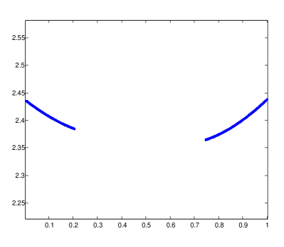
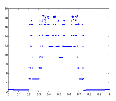
Figure 6. Numerically evaluated cost function $E(x)$ for exponentially distributed H. Right display shows also results for chaotic region (stopped after a fixed number of iterations). Left display is a magnification of the right one, showing only the results over the region of monotonicity.

The monotonicity of the cost over the left and right intervals is apparent. The separatrix ${\mathcal{S}}$ intersects the ray of initial conditions ${\mathbf{r}}$ at two points, $x_{+}\approx 0.7465...$ and $x_{-}\approx.1954...$ (compare with Figure 4). Between the points, the initial conditions are in the chaotic region. The monotonicity of $E$ outside of the chaotic region means that one of the two initial values, $x_{+}$ or $x_{-}$ should generate the optimal trajectory. Numerically, $x_{+}$ wins: $E(x_{+})\approx 2.3645<E(x_{-})\approx 2.3861$.

8. Conclusion

We developed a geometric approach to the Linear Search Problem via discrete time Hamiltonian dynamics, which explains some of the hidden structure of the cost function. The rapid decay of the tail distribution function translates into hyperbolicity of the underlying Hamiltonian dynamics. The latter is defined by the variational recursion which plays a key role in the characteristics of the optimal search trajectory. In particular, hyperbolicity implies the existence of separatrix which divides the regular and chaotic regions, and the optimal search trajectory needs to start on the separatrix: the chaotic region cannot contain optimal orbits, while in the regular region the orbits father away from separatrix have higher cost (monotonicity of the cost function).

While this scenario is proved in this note only for a specific case of exponential tail distribution function, we anticipate that for other distributions with sufficiently fast decay, the same type of results, including the existence of separatrix and monotonicity of cost function in the region of monotonicity, will hold. Some of this hope is supported by partial results, see the appendix.

We plan to return to this more general classes of distributions in a follow-up paper, where we also plan to address the phenomenon of separatrix slow-down (the growth of trajectories on separatrix is slower than that in the interior of the region of monotonicity).

There are other open questions arising in the context of Hamiltonian dynamics based approach to the search problem. Extending the set of analyzed distributions to those with bounded support is a natural task.

We also expect that in the search on rays, where the corresponding Hamiltonian map is higher dimensional, hyperbolicity will also play an important role and higher dimensional separatrix (unstable manifold) can be found. It is expected that optimal search plan would still be restricted to the unstable manifold.

Appendix A Series expansions

The expansion near $x=\infty$ for the separatrix given by

$$\phi(x-\phi(x))=\ln(x)$$

leads to logarithmic series

$$\phi(x)=\sum_{n=0}^{\infty}\frac{Q_{n}(\ln(x))}{x^{n}}.$$

The first three terms are given by

$$\phi(x)=\ln(x)+\frac{\ln(x)}{x}+\frac{1}{x^{2}}\left(\frac{1}{2}+\frac{3}{4}\ln(x)-\frac{1}{3}\ln^{2}(x)\right)+...$$

To justify this expansion, we need

Lemma 2.

The equation $x=t(x)-\ln t(x)$ has a smooth solution for sufficiently large $x$

$$t(x)=x+\ln x+O\left(\frac{\ln x}{x}\right).$$

Proof.

Let us write

$$t(x)=x+\ln x+r(x)$$

and substitute in the equation. After some simplifications, we have

$$r=\ln\left(1+\frac{\ln x}{x}+\frac{r(x)}{x}\right).$$

Application of the contraction mapping principle to $r(x)$ gives the required error estimate. ∎

Now, we prove

Proposition 11.

$$\phi(x)=\ln x+O\left(\frac{\ln x}{x}\right).$$

Proof.

Consider the first two iterations by ${\bf R}^{-1}$ of $\phi_{0}:=(x=t,y=0)$,

$$\phi_{1}:=(x=t,y=\ln t),\phi_{2}:=(x=t-\ln t,y=\ln t).$$

They can be represented as graphs $y=\phi_{1}(x),y=\phi_{2}(x)$ for sufficiently large $x$. Note that $\phi_{1}(x)=\ln(x)$, while $\phi_{2}(x)=\ln t(x)$, where $x=t(x)-\ln t(x)$.

Now, using the above lemma we estimate

$$|\phi_{2}(x)-\phi_{1}(x)|=|\ln t(x)-\ln x|=|\ln\left(x+\ln x+r(x)\right)-\ln x|=\left|\ln\left(1+\frac{\ln x}{x}+\frac{r(x)}{x}\right)\right|\leq C\,\frac{\ln x}{x}$$

Applying contraction mapping principle, we obtain the desired estimate

$$|\phi(x)-\ln x|\leq C\,\frac{\ln x}{x}.$$

∎

Theorem 1.

The mapping R restricted to the separatrix takes the form

$$x_{n+1}=x_{n}+\ln(x_{n})+O(\ln(x_{n})/x_{n})$$

Proof.

The separatrix is given by

$$\phi(x)=\ln(x)+\rho\left(\frac{\ln(x)}{x}\right)$$

for $x\rightarrow\infty$.

Then, using the forward map representation $(x_{n+1},y_{n+1})=(\exp y_{n},x_{n+1}-x_{n})$, we have

$$\ln(x_{n+1})+\rho(x_{n+1})=x_{n+1}-x_{n},$$

where $\rho(x)=O(\ln x/x)$ is a smooth function. Applying the implicit function theorem and estimating the error term, we obtain the result.

∎

Theorem 2.

The asymptotics of the mapping restricted to the separatrix is given by

$$x_{n}=n(\ln(n)+\ln(\ln(n)))+r_{n},$$

where $r_{n}$ is a sequence satisfying

$$|r_{n+1}-r_{n}|\leq C.$$

Proof.

Substitute the expansion of $x_{n}$ in the recurrent relation

$$x_{n+1}=x_{n}+\ln(x_{n})+O(\ln(x_{n})/x_{n}),$$

then after some cancellations, we obtain that $r_{n+1}=r_{n}+1+O(1)$ which implies the result. ∎

Appendix B Two-sided Gaussian distribution: Beck-Bellman problem

We consider the two-sided search on the real line with Gaussian probability distribution function as in the original Beck-Bellman problem and we show numerically that the same canonical structure persists: separatrix intersecting the curve of initial turning points.

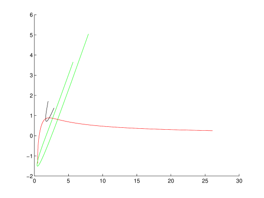
Figure 7. Invariant curve and iterated initial data in Beck’s problem. The long curve is invariant manifold. The other two bended curves are 1st and 2nd forward iterates of initial data. The initial data itself is not present because continuation of the separatrix in that region is computationally too difficult.

The difference relation obtained in [7], is given by

$$(x_{n}+x_{n+1})\phi(x_{n})=G(x_{n})+G(x_{n-1}),$$

where

$$\phi(t)=\frac{1}{\sqrt{2\pi}}e^{-t^{2}/2},\,\,\,\,G(x)=\int_{x}^{\infty}\phi(t)dt.$$

The actual turning points are $(-1)^{n}x_{n},$ while $x_{n}\geq 0$. For matlab computations, we use

$${\rm erfc(x)}=\frac{2}{\sqrt{\pi}}\int_{x}^{\infty}e^{-t^{2}}dt$$

and the inverse function called ${\rm erfcinv}$. Using the relation

$$G(x)=\frac{1}{2}\rm erfc(x/\sqrt{2}).$$

the finite difference relation takes the form

$$(x_{n+1}+x_{n})\phi(x_{n})=\frac{1}{2}(\rm erfc(x_{n}/\sqrt{2})+\rm erfc(x_{n-1}/\sqrt{2})).$$

Now, using $y_{n+1}=x_{n+1}-x_{n}$, we have

$$x_{n+1}=\frac{1}{2\phi(x_{n})}({\rm erfc}(x_{n}/\sqrt{2})+{\rm erfc}((x_{n}-y_{n})/\sqrt{2}))-x_{n}.$$ (13)

We will also use the inverse map which takes the form

$$x_{n+1}=x_{n}-y_{n}$$

$$y_{n+1}=x_{n+1}-\sqrt{2}\,{\rm erfcinv}\,(2\phi(x_{n+1})(x_{n}+x_{n+1})-{\rm erfc}(x_{n+1}/\sqrt{2})).$$

In this case, the initial data is given by the line segment $x_{1}=y_{1}=t$.

Appendix C Gaussian tail distribution. One-sided search.

In this section we verify that contraction mapping principle can be used to establish existence of separatrix for the one-sided search problem with Gaussian tail distribution.

In this case $f(x)=e^{-x^{2}}$, so that the second order difference relation is given by

$$x_{n+1}=\frac{1}{2x_{n}}\,e^{\,x_{n}^{2}-x_{n-1}^{2}}.$$

Let $y_{n+1}=x_{n+1}^{2}-x_{n}^{2}$, then we have

$$x_{n+1}=\frac{1}{2x_{n}}e^{y_{n}}$$

$$y_{n+1}=x_{n+1}^{2}-x_{n}^{2}.$$

We will also need the inverse map

$$x_{n}=\sqrt{x_{n+1}^{2}-y_{n+1}}$$

$$y_{n}=\ln{(2x_{n}x_{n+1})}$$

In this case, the initial data is given by a quadratic curve

$$y=x^{2}=t^{2}.$$

Now, we show that the contraction principle can be extended to Gaussian case.

Theorem 2 (Unstable invariant manifold for one-sided Gaussian).

There exists an invariant manifold containing a graph $y=h(x)$ on $x\in[x_{0},\infty)$ and with

$$|h(x)-\ln(2x^{2})|<1.$$

Proof.

Set up contraction mapping

$$\Phi(\phi)(x)=\ln(2z_{\phi}(x)x),$$

where

$$z^{2}_{\phi}(x)-\phi(z_{\phi}(x))=x^{2}.$$

Let

$${\bf X}=\{\phi\in C^{1}(x_{0},\infty),\phi(x)>0,0<\phi^{\prime}(x)\leq 1/2\}.$$

By applying the same argument as in the exponential case, we can ensure that $\Phi$ leaves ${\bf X}$ invariant if we take as the initial guess $\phi_{0}(x)=\ln(2x^{2})$.

To establish contraction, consider

$$|\Phi(\phi)(x)-\Phi(\psi)(x)|=|\ln(2xz_{\phi}(x))-\ln(2xz_{\psi}(x))|=$$

$$|\ln(z_{\phi}(x))-\ln(z_{\psi}(x))|\leq\frac{1}{\min(z_{\phi}(x),z_{\psi}(x))}|z_{\phi}(x)-z_{\psi}(x)|.$$

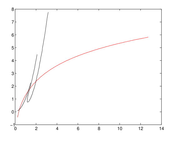
Figure 8. Invariant curve and iterated initial data.The longer curve is the invariant manifold. Two other curves are iterated initial turning points.

Using the identity

$$z_{\phi}^{2}(x)-z_{\psi}^{2}(x)=\phi(z_{\phi}(x))-\psi(z_{\psi}(x)),$$

and that $z_{\phi}(x)\geq x$, we have

$$|z_{\phi}(x)-z_{\psi}(x)|\leq\frac{1}{z_{\phi}(x)+z_{\psi}(x)}|\phi(z_{\phi}(x))-\psi(z_{\psi}(x))|$$

$$\leq\frac{1}{2x}(|\phi(z_{\phi}(x))-\psi(z_{\phi}(x))|+|\psi(z_{\phi}(x))-\psi(z_{\psi}(x))|$$

$$\leq\frac{1}{2x}\left(||f-g||+||g^{\prime}||\cdot|z_{\phi}(x)-z_{\psi}(x)|\right).$$

Combining the terms, we have

$$|z_{\phi}(x)-z_{\psi}(x)|\leq\frac{1}{2x-||{\psi}^{\prime}||}\,||\phi-\psi||$$

and then

$$|\Phi(\phi)(x)-\Phi(\psi)(x)|\leq\frac{1}{2x}\cdot\frac{1}{2x-||\psi^{\prime}||}\,||\phi-\psi||.$$

Since we have assumed the bound $0<{\psi}^{\prime}<1/2$, taking $x\geq 1$, we obtain contraction

$$|\Phi(\phi)(x)-\Phi(\psi)(x)|\leq\frac{1}{3}\,||\phi-\psi||.$$

∎

References

- [1] S. Alpern, A. Beck, Asymmetric rendezvous on the line is a double linear search problem, Math. Oper. Res. 24 (1999), no. 3, 604–618.
- [2] S. Alpern, S. Gal, The theory of search games and rendezvous. Springer 2003.
- [3] S. Aubry, P.Y. Le Daeron, The discrete Frenkel-Kontorova model and its extensions, Physica D 8 (1983) 381-422.
- [4] Y. Baryshnikov, E. Coffman, P. Jelenkovich, P. Momcilovic, D. Rubenstein, Flood search under California split rule, Oper. Res. Lett. 32 (2004) 199–206.
- [5] R. Bellman, Problem 63-9*, SIAM Review, 5(2), 1963.
- [6] A. Beck, On the linear search problem, Isr. Jour. of Math. 2 (1964) 221-228.
- [7] A. Beck and M. Beck, Son of the linear search problem, Isr. J. Math. 48 (1984) 109-122.
- [8] A. Beck, M. Beck, The revenge of the linear search problem, SIAM J. Control Optim. 30 (1992) no. 1, 112–122.
- [9] A. Beck, M. Beck, The linear search problem rides again, Isr. J. Math 53 (1986) 365–372.
- [10] A. Beck, D.J. Newman, Yet more on the linear search problem, Israel J. Math. 8 (1970) 419–429.
- [11] W. Franck, An optimal search problem, SIAM Review Vol. 7, No. 4 (1965) 503-512.
- [12] W.S. Lim, S. Alpern, A. Beck, Rendezvous search on the line with more than two players, Oper. Res. 45 (1997) no. 3, 357–364.
- [13] I.R. De Pablo, A. Becker, T. Bretl, An optimal solution to the linear search problem for a robot with dynamics, Intelligent Robots and Systems (IROS), 2010.
- [14] M-Y Kao, J.H. Reif, S.R. Tate, Searching in an Unknown Environment: An Optimal Randomized Algorithm for the Cow-Path Problem, Proceedings of SODA’1993. pp.441 447
- [15] A. Katok, B. Hasselblatt, Introduction to the modern theory of dynamical systems, CUP, Cambridge, 1995.