Latent protein trees

Abstract

Unbiased, label-free proteomics is becoming a powerful technique for measuring protein expression in almost any biological sample. The output of these measurements after preprocessing is a collection of features and their associated intensities for each sample. Subsets of features within the data are from the same peptide, subsets of peptides are from the same protein, and subsets of proteins are in the same biological pathways, therefore, there is the potential for very complex and informative correlational structure inherent in these data. Recent attempts to utilize this data often focus on the identification of single features that are associated with a particular phenotype that is relevant to the experiment. However, to date, there have been no published approaches that directly model what we know to be multiple different levels of correlation structure. Here we present a hierarchical Bayesian model which is specifically designed to model such correlation structure in unbiased, label-free proteomics. This model utilizes partial identification information from peptide sequencing and database lookup as well as the observed correlation in the data to appropriately compress features into latent proteins and to estimate their correlation structure. We demonstrate the effectiveness of the model using artificial/benchmark data and in the context of a series of proteomics measurements of blood plasma from a collection of volunteers who were infected with two different strains of viral influenza.

, , , , and

t1This work was partially done when the author was a Ph.D. candidate at the Technical University of Denmark. t2Supported by the Defense Advanced Research Projects Agency (DARPA), number lN66001-07-C-0092 (G.S.G.).

1 Introduction

Unbiased, label-free, mass spectrometry proteomics,sometimes called “shotgun” proteomics, is a technique for measuring nearly all abundant proteins in a biological sample. Because of numerous technical advances it is becoming increasingly robust and sensitive, leading to greater effectiveness for the study of biological and medical questions [Aebersold and Mann (2003), Service (2008), Ping (2009)]. While early work in this field met with a number of notorious failures [Petricoin et al. (2002), Baggerly et al. (2004), Zhang and Chan (2005)] due to overlapping peaks, batch effects and systematic noise, high accuracy spectrometers along with multiple fractionation techniques such as liquid chromatography and ion mobility have led to increased robustness as well as improved qualitative and quantitative results.

After summarization, data generated by this technology is typically presented as a $p\times n$ dimensional matrix of real-valued intensities where the number of measured features $p$ is typically orders of magnitude larger than $n$, as in microarray gene expression data. However, there are a number of important characteristics that distinguish mass spectrometry proteomics from gene expression data. First, each feature is a short peptide that has been enzymatically cut out of a parent protein, and parent proteins typically give rise to many such peptides. Second, only the more abundant of these features are typically identified (meaning that the peptide sequence and originating protein are known). Third, features that are present at lower abundances will typically have numerous missing values across the samples. Finally, while the error rate for assigning identifications to features is low, it is not zero, and this leads to some peptides with incorrect identifications.

Analysis approaches for these data can be performed at the feature level or at the protein level. The obvious consequence of performing analysis at the feature level is a significant loss of power due to the highly dependent nature of subsets of the features—particularly those that originate from the same protein. We prefer a dimension reduction approach in which groups of features are collected and summarized prior to analysis of associations between features and biological phenotypes. There are a number of approaches to this in the literature, almost all of which rely entirely on the identified features in the data set.

The simplest of these approaches involves direct summarization of all or some features that are identified for each protein either through averaging or robust summarization based on quantiles [Polpitiya et al. (2008)]. There are also a number of regression approaches which include fixed effects for protein, peptide and experimental group [Karpievitch et al. (2009)], include an additional random effect for situations in which subjects are measured in replicate [Daly et al. (2008)], or add additional interaction effects between treatment and features [Clough et al. (2009)]. These may assume constant or varying noise levels across isotope groups and have been shown in some cases to exhibit better performance than naive summarization approaches that do not adjust for confounding factors [Clough et al. (2009)].

We are aware of only one approach to the analysis of these data that examines correlation structure between data features [Lucas et al. (2012)]. This approach utilizes a latent factor model to aggregate features and uses priors on the loadings that are informed by identifications. This leads to aggregation of multiple features into “metaproteins.” This is a sparse factor modeling approach where nonzero loadings for factor $i$ are biased toward features that are identified as originating from protein $i$. While this approach allows the utilization of unidentified features in the data, it fails to account for correlation structure that arises when multiple proteins are involved in the same pathways.

In this paper we present an extension of Lucas et al. (2012) that explicitly models correlation structure between factors. We do this by incorporating a hierarchical structure on the latent metaproteins that allows borrowing strength between factors to estimate overall factor scores. We demonstrate improvements over both a generic sparse factor model [Carvalho et al. (2008)] and the earlier proteomics factor model [Lucas et al. (2012)], in terms of accuracy of factor estimates and eventual association with biological phenotypes. Finally, we demonstrate the incorporation of known correlation structure in the form of time series measurements in our analysis of a viral challenge data set in Section 7.

2 Motivating data

While the specifics of data generation may vary at different proteomics laboratories, the model we describe is appropriate for any high-accuracy mass spectrometry data. In general, the steps to data generation are as follows: (i) a biological sample is distilled to a solution containing those proteins that are of interest; (ii) the proteins in the sample are then broken up via trypsin; (iii) the processed sample is separated according to hydrophobicity using liquid chromatography. The time at which a particular constituent of the sample passes out of the chromatography column is called the retention time; (iv) an electric charge is induced on the peptides; (v) the mass and intensity of these ions is measured in a mass analyzer. The intensity and ion masses are measured at a regular interval, called the sampling rate, and the resulting measurements form a trace with visible peaks, called features, that correspond to one or more peptides. Because the sampling rates are high relative to the size of these features, each feature spans a range of mass-to-charge ratios and retention times.

In nature, approximately 1% of all Carbon atoms are Carbon-13 (they contain an extra neutron). This leads to multiple features per peptide, each one containing a different integer number of Carbon-13 atoms. These are collected into a single isotope group (IG) during preprocessing, and the intensity of this isotope group is estimated as the total volume under its associated features. In addition to multiple features from Carbon-13 substitution, a peptide may be present in the data set multiple times at different charge states. These different charge states will have different mass to charge ratios and therefore result in multiple isotope groups per peptide.

There are inherently two different types of correlation present in label-free, unbiased proteomics data. First, each isotope group originates from a particular protein and there are typically many isotope groups per protein in the data set—particularly for proteins that are highly abundant and/or of large molecular weight in the original sample. Second, some collections of proteins are expected to behave similarly because they are part of the same biological pathways. This will result in correlation between proteins (and therefore correlation between isotope groups) that are of distinct etiology. In general, distinct sources of correlation are confounding without some additional information allowing us to distinguish them. In the case of proteomics, there are techniques for identifying the specific amino acid sequence of a subset of the isotope groups that are present at relatively high concentrations. These sequences are then associated to particular proteins through sequence alignment to proteins in a database [Nesvizhskii et al. (2003)]. We have then, for a limited subset of the isotope groups, a (possibly imperfect) peptide sequence and originating protein, which we call an annotation.

The proteomics data we will be focused on was obtained from 43 patients as part of the DARPA H1N1/H3N2 viral challenge project [Zaas et al. (2009)]. From the entire pool, 24 patients were exposed to H1N1 and 17 were exposed to H3N2. For each patient, four samples were taken at different reference time points, baseline ($t=0$), the time of maximum symptoms ($t=1$) as well as $t=0.2$ and $t=0.8$. Each subject was labeled as symptomatic (SX) or asymptotic (ASX) based on self-reported symptom scores, as well as viral culture. The samples of the H3N2 study were run in two batches with the initial pilot study containing only samples from time points $t=\{0,1\}$ and the followup containing the $t=\{0.2,0.8\}$ samples. In summary, we have $N=172$ samples from two studies (H1N1 and H3N2) divided in three batches (H1N1, H3N2₁ and H3N2₂), two conditions (SX and ASX) where fortunately the batches and conditions are not confounded. The data itself is a matrix containing expression values for approximately 40,000 different IGs. Peptide annotation was done using a combination of Mascot and PeptideProphet algorithms [Keller et al. (2002), Perkins et al. (1999)]. Nearly 85% of the IGs remained unannotated. Since H1N1 and H3N2 are two different experiments, their annotation set is substantially different, thus, an alignment algorithm must be used in order to take advantage of as much annotated data as possible, otherwise we will be forced to use only those IGs shared by both data sets (1697 IGs). Isotope groups from the three batches were aligned using the algorithm described in Lucas et al. (2012). From all IGs, 13,845 were successfully aligned across the H1N1 and H3N2 data sets. From the set of 4670 annotated IGs, only 1697 had annotations in both data sets. The set of annotations consists of 239 proteins from which 106 are assigned to more than one IG. The data has a relatively low overall missingness rate, most of them among low abundance IGs. However, missing values are unevenly distributed: H3N2₁ having $10.3\%$ missingness, H3N2₂ $0.7\%$ and H1N1 up to $2.5\%$. Two samples were removed from subsequent analysis because they had more than $30\%$ missing values in the set of annotated IGs.

3 Model definition

We model a sample $n$ of batch $m$ consisting of $p$ IG expressions, ${\mathbf{x}}_{n}^{m}$, as an extended factor model separated into four effects, namely, batch, systematic, protein expression and noise,

$${\mathbf{x}}_{n}^{m}=\bolds{\mu}^{m}+{\mathbf{A}}{\mathbf{z}}_{n}+{\mathbf{B}}{\mathbf{w}}_{n}+\bolds{\varepsilon}_{n},$$ (1)

where ${\mathbf{x}}_{n}^{m}$, $\bolds{\mu}^{m}$, ${\mathbf{z}}_{n}$, ${\mathbf{w}}_{n}$ and $\bolds{\varepsilon}_{n}$ are $p\times 1$ vectors. In particular, $\bolds{\mu}^{m}$ is the mean expression vector of batch $m$, factors ${\mathbf{z}}_{n}=[z_{1n}\enskip\cdots\enskip z_{N_{F}n}]^{\top}$ are meant to capture $N_{F}$ systematic effects, ${\mathbf{w}}_{n}$ is the expression level of $N_{P}$ proteins for sample $n$, ${\mathbf{A}}$ and ${\mathbf{B}}$ are $p\times N_{F}$ and $p\times N_{P}$ loading matrices for the systematic effects and protein expressions, respectively, and $\bolds{\varepsilon}_{n}$ is measurement idiosyncratic noise. Systematic effects are included in the model for the sole purpose of cleaning the data as much as possible from batch effect specific and technical noise, with the aim to obtain protein profiles $\{{\mathbf{w}}_{n}\}$, that better reflect true biology rather than technical variability. Provided that protein expression is not directly observed and because profile vectors $[w_{k1}\enskip\cdots\enskip w_{kN}]$ are likely to be estimated from IGs that belong to multiple proteins, from now on we refer to them as latent proteins. A priori, we let each IG be associated only to a single latent protein, say, $k$, meaning that each row of ${\mathbf{B}}$ contains just one nonzero entry.

Identifiability issues in the model of (1) are minimized for three reasons: (i) confounding between systematic effects and metaproteins is very unlikely because ${\mathbf{A}}$ is dense and ${\mathbf{B}}$ is highly sparse. (ii) ${\mathbf{w}}_{n}$ does not have a sign ambiguity because ${\mathbf{B}}$ has only nonnegative entries. (iii) ${\mathbf{z}}_{n}$ can be identified up to scale and permutations as long as its distribution is non-Gaussian [see Kagan, Linnik and Rao (1973)]. Scale and permutation ambiguities are not of great concern here because we are not interested in the interpretation of systematic effects. Besides, in a case in which batch effects fully correlate with biological effects, our model will model them jointly as batch effects. This type of batch confounding is reasonably common in high-throughput data [Leek et al. (2010)], and the failure of our model to find biological effects when those effects are heavily confounded with batch is the desired behavior.

3.1 Prior specification

We need to specify prior distributions for each one of the elements in the right-hand side of (1). Measurement noise is set to a zero-mean Gaussian with diagonal covariance matrix $\bolds{\Psi}$, to allow for different noise variances for each IG. Entry specific priors for $\bolds{\Psi}$ are set to flat inverse gamma distributions with shape $t_{s}=1.1$ and rate $t_{r}=0.001$, the former to keep the variance bounded away from zero. Mean batch effects have Gaussian priors with mean $t_{m}=8$ and small precision $t_{p}=0.01$, set mainly based on the overall mean expression of the data. Missing values are provided with independent standardized Gaussian distributions in order to favor small values. This reflects the fact that missing values are mostly due to low abundance peptides.

3.1.1 Systematic effects

We define systematic effect as a portion of variability expressed in a large collection of isotope groups that cannot be classified either as nonspecific measurement noise or biological variability, meaning that it is more likely due to technical variability. These effects are usually characterized by high levels of correlation across many isotope groups, but potentially only in a subset of the samples (e.g., only those in one batch). We capture the first part through the use of independent Gaussian priors on the elements of ${\mathbf{A}}$, which allows systematic effects to span the entire set of isotope groups. Aiming to allow individual samples to be largely dropped from specific systematic factors, we utilize independent Laplace priors for the elements of ${\mathbf{z}}_{n}$. These are parameterized as scale mixtures of Gaussians with exponential mixing densities to facilitate inference [Henao and Winther (2011)]. We consider that the number of systematic factors $N_{F}$ is not critical because we are not concerned about the interpretability of matrix ${\mathbf{A}}$. Besides, we have observed empirically that the variance explained by the systematic effect factors saturates quickly as $N_{F}$ increases. However, we decided to place an automatic relevance determination (ARD) prior on ${\mathbf{A}}$ [Neal (1996)]. In particular, being $a_{ij}$ and $z_{jn}$ elements of ${\mathbf{A}}$ and ${\mathbf{z}}_{n}$, respectively, we have

where $\rho_{j}$ is a shared factor-wise variance for the columns of ${\mathbf{A}}$ and $\tau_{jn}$ is an auxiliary variance with exponential mixing so, marginally, $z_{jn}\sim\operatorname{Laplace}(\lambda^{2})$ [Andrews and Mallows (1974)]. We further place a gamma hyperprior on the rate of the Laplace distribution with parameters $\ell_{s}=4$ and $\ell_{r}=2$. The ARD is a variable selection prior; Large values of $\rho_{j}$ will correspond to small values of the $j$th column of ${\mathbf{A}}$, thus virtually switching off the entire effect. Setting $r_{r}=1.1$ and $r_{s}=0.001$ will encourage the desired behavior. In practice, the effective number of factors can be determined by thresholding $\rho_{j}$ or the elements of ${\mathbf{A}}$ column-wise.

3.1.2 Latent protein profiles

We make two assumptions regarding isotope group expression. One is that each isotope group originates from only one latent protein and the other is that latent proteins may correlate with each other due to biological pathway activity. To model the first feature, we set a prior hierarchy as follows:

$$b_{i,u_{i}}|u_{i}\sim\mathcal{N}_{+}(0,1),\qquad u_{i}|{\mathbf{v}}_{i}\sim\operatorname{Discrete}({\mathbf{v}}_{i}),\qquad{\mathbf{v}}_{i}|\alpha\sim\operatorname{Dirichlet}(\alpha{\mathbf{1}}_{N_{P}}),$$

where $b_{i,j}=0$ if $j\neq u_{i}$, $\mathcal{N}_{+}(\cdot)$ is the Gaussian distribution truncated below zero and where the $i$th IG is associated with the latent protein indexed by $u_{i}$ with probability ${\mathbf{v}}_{i}$. This means that vector ${\mathbf{u}}$ serves as a labeling variable for IGs. The conjugate prior for the vector of $N_{P}$ probabilities, ${\mathbf{v}}_{i}$, is set using a shared concentration $\alpha$. For the latter, we provide a flat gamma prior with parameters $a_{s}=1$ and $a_{r}=1$ [see Escobar and West (1995)].

We know that groups of proteins might have similar expression profiles for different reasons, for example, because they are structurally similar, mediate similar biological processes, share a pathway, etc. In order to capture this structure, we place a prior over binary trees on the $N_{P}$ latent proteins. This allows us to model correlation among metaproteins and leads to an interpretable representation of isotope groups, latent proteins and their interactions. Figure 1 illustrates the concept for a particular setting with $p=15$ IGs distributed in $N_{P}=5$ proteins. We can see a hierarchical clustering structure in which, for instance, latent proteins $w_{1}$ and $w_{2}$ are more similar than $w_{4}$ and $w_{5}$, thus more correlated. The pseudo time $t_{j}$ at which two nodes merge into $v_{j}$ acts as a similarity measure so that more alike latent proteins merge sooner in time, allowing us to directly quantify their pairwise or group-wise similarities. The proposed hierarchy is an implementation of the Kingman’s coalescent [Kingman (1982a)] and reflects the idea that isotope groups and latent proteins lay in different levels and that protein pathways are proxies for the average profiles of collections of proteins.

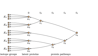
Figure 1: Latent protein tree structure. Particular tree with $N_{P}=5$ and three isotope groups assigned to each latent protein. The pseudo time variable $t$ defines the merging points.

Given a tree structure, $\{{\mathbf{t}},\bolds{\pi}\}$, where ${\mathbf{t}}$ is the vector of merging times and $\bolds{\pi}$ is the set of partitions at each level of the tree, we specify the relationship between node $v_{j}$ and its parent node $n_{k}$ (or $w_{k}$ at the leaves) through a multivariate Gaussian transition probability and set the following prior hierarchy:

$$\quad{\mathbf{v}}_{j}|{\mathbf{v}}_{k},t_{j},t_{k},\bolds{\Phi}\sim\mathcal{N}\bigl{(}{\mathbf{v}}_{k},(t_{k}-t_{j})\bolds{\Phi}\bigr{)},\qquad\{{\mathbf{t}},\bolds{\pi}\}\sim\operatorname{Coalescent}(N_{p}),$$ (3)

where ${\mathbf{v}}_{j}$ is a $N$-dimensional row vector and $\bolds{\Phi}$ is a covariance matrix encoding the correlation structure in ${\mathbf{v}}_{j}$. A coalescent prior selects a pair to merge uniformly from partition $\pi_{j}$ and sets merging times with rate 1, this is $t_{k}\sim\operatorname{Exponential}(1)$. With no further constraints, this prior distribution leads to a uniform prior distribution over trees that is independent of merging times and is infinitely exchangeable [Kingman (1982a, 1982b)]. Different priors for $\bolds{\Phi}$ add flexibility to the model, for example, in the i.i.d. case, a diagonal $\bolds{\Phi}$ with independent inverse gamma prior distributions on each diagonal element will accommodate for differing levels of noise for different samples. In cases where there is known structure, a different prior could be used. In our analyses we use inverse Wishart priors to model correlation due to sample replicates and Gaussian process priors for smoothness in time series data. Inference for hierarchy in (3) is carried out using an efficient sequential Monte Carlo Sampler introduced by Henao and Lucas (2012).

3.2 Inference

Model fitting is performed using Markov chain Monte Carlo (MCMC) to collect samples from the posterior of all parameters in the model, namely, $\bolds{\mu}^{m}$, ${\mathbf{A}}$, ${\mathbf{z}}_{n}$, ${\mathbf{B}}$, ${\mathbf{w}}_{n}$, $\bolds{\Psi}$, ${\mathbf{u}}$, $\bolds{\pi}$ and $\bolds{\Phi}$. The most relevant summaries involve posterior samples from the latent proteins, IG-protein assignments and the hierarchical structure encoded by the binary tree, $\bolds{\pi}$. Nearly all quantities of interest are updated using Gibbs sampling except for the tree components that require sequential Monte Carlo (SMC) sampling. In all the experiments described in this paper we set the hyperparameters of the model to the values already mentioned unless otherwise stated. The upper bound for the number of factors is set to a conservatively large value; we have observed in practice that $N_{F}=\lfloor 2\log(p)\rfloor$ is large enough. For tasks with $p$ and $N$ in the lower thousands and hundreds, respectively, we can expect the inference routine to take less than a couple of hours in a desktop machine. The entire sampling sequence is fully described in the Appendix.

Summaries for most of the important quantities of the model are computed in the usual way by means of histograms and empirical quantiles. Summarizing trees, on the other hand, is not such an easy task because tree averaging is not a well-defined operation. We could, in principle, use the pseudo time variable to build a pairwise distance matrix between latent proteins and then attempt to build a tree from a summary of such a similarity matrix. The problem being that we do not have any guarantee that this average of binary trees will produce a binary tree as well. We tried this approach with both artificial and real data, and found that the tree built using means or medians of the similarity matrices collected during inference oftentimes produced trees with nonbinary branching, thus not matching the prior assumption. In view of this, we decided to select a single tree from all the available samples using as criterion the marginal likelihood of the tree. This is a common practice in tree based models; see, for instance, Teh, Daume III and Roy (2008) and Adams, Ghahramani and Jordan (2010).

The source code and demo scripts for the model presented in this paper are written in MATLAB and C, and have been made publicly available at http://www.duke.edu/~rh137/files/lpt_v0.3.tar.gz.

4 Artificial data

We begin with a set of experiments using artificially generated data in order to illustrate some of the features of our model and to perform some quantitative comparisons. We generated two data sets $D_{1}$ and $D_{2}$ of sizes $\{p,N,N_{B},N_{F},N_{P}\}=\{800,80,2,4,32\}$ and $\{1600,80,3,6,64\}$, respectively. Denoting the elements of $\bolds{\mu}^{m}$, ${\mathbf{A}}$, ${\mathbf{B}}$ and $\bolds{\Psi}$ as $\mu_{i}^{m}$, $a_{ij}$, $b_{ik}$ and $\psi_{i}$, respectively, we draw $N$ observations of the model from the following hierarchy:

$${\mathbf{x}}_{n}^{m} \sim \mathcal{N}\bigl{(}\bolds{\mu}^{m},\bolds{\Sigma}\bigr{)},$$

$$\mu_{i}^{m} \sim \mathcal{N}(8,2),\qquad m\sim\operatorname{Discrete}\bigl{(}N_{B}^{-1}{\mathbf{1}}_{N_{B}}\bigr{)},$$

$$a_{ij} \sim \mathcal{N}(0,0.1),$$

$$b_{i,u_{i}} \sim \mathcal{N}_{+}(0,1),\qquad u_{i}\sim\operatorname{Discrete}({\mathbf{v}}),$$

$$\psi_{i}^{-1} \sim \operatorname{Gamma}(1.1,0.02),\qquad{\mathbf{v}}\sim\operatorname{Dirichlet}(\bolds{\alpha}),$$

$${\mathbf{S}}^{-1} \sim \operatorname{Wishart}({\mathbf{I}},N_{P}),\qquad\bolds{\alpha}\sim\operatorname{Uniform}(0.8,2.4),$$

where $\bolds{\Sigma}={\mathbf{A}}{\mathbf{A}}^{\top}+{\mathbf{B}}{\mathbf{S}}{\mathbf{B}}^{\top}+\bolds{\Psi}$, ${\mathbf{A}}$ is a $p\times N_{F}$ matrix of systematic factor loadings, ${\mathbf{B}}$ is a $p\times N_{P}$ matrix of latent protein loadings, ${\mathbf{S}}$ is the covariance matrix of the latent protein profiles and $\bolds{\Psi}$ is the noise diagonal covariance matrix, as in (1). We generated 50 replicates of each data set and uniformly flagged 20% of its values as missing. We ran our sampler for 4000 iterations, using the first 3000 as burn-in period. For this experiment, we set the distribution of the systematic factors to Gaussian, to match the assumption made in $\bolds{\Sigma}$. Since we are not introducing correlation across samples, we set $\bolds{\Phi}$ to diagonal with independent gamma priors. The average number of systematic factors is selected with threshold $\rho_{j}<10^{3}$. We label each latent protein by tabulating the IGs associated to it from vector ${\mathbf{u}}$ and then picking the label having maximum count. We define identity as the percent of correctly labeled latent proteins and confusion as the percent of variables incorrectly associated to their latent proteins. We compare our model (LPT) with (i) its simplified version without the tree structure inference we call sLPT, thus without covariance structure in the latent profiles [Lucas et al. (2012)]. Table 1 shows results for the structural components of the model—identity, confusion and number of systematic factors. Results demonstrate that the model is able to capture the association between IGs and latent protein profiles through ${\mathbf{u}}$ while properly handling “batch” effects and missingness in the data. The two methods perform similarly because estimates of systematic effects and peptide-protein associations is only weakly influenced by the protein tree structure. Even so, LPT performs slightly better than sLPT in terms of protein association accuracy.

=300pt Set Method $\bolds{N_{F}}$ Identity Confusion $D_{1}$ LPT 4 $\bolds{(3,7)}$ 0.97 $\bolds{(0.94,1.00)}$ 0.002 $\bolds{(0.000,0.009)}$ sLPT 4 $\bolds{(3,7)}$ 0.97 $(0.91,1.00)$ 0.005 $(0.000,0.016)$ $D_{2}$ LPT 6 $\bolds{(5,10)}$ 0.98 $\bolds{(0.97,1.00)}$ 0.003 $\bolds{(0.00,0.008)}$ sLPT 6 $(5,10)$ 0.97 $(0.93,1.00)$ 0.007 $(0.001,0.014)$

Table 1: Structural measures for artificial data. $N_{F}$ is selected with threshold $\rho_{j}<10^{3}$. Pairs in brackets are empirical 90% intervals across replicates. Best results in boldface letters

We can also assess the performance of our model in terms of covariance matrix and missing value estimation. We compare LPT and sLPT as well as a sparse factor model as proposed by Carvalho et al. (2008), sFM, which utilizes the same priors for missing values and batch effects used by our model. For sFM we set the number of factors to $N_{F}+N_{P}=\{21,24\}$, accordingly. In principle, the sparse model is flexible enough to estimate ${\mathbf{A}}$ and ${\mathbf{B}}$ but not ${\mathbf{S}}$, for the model assumes independent profiles, similar to sLPT. Table 2 shows summaries of mean square error (mse), mean absolute error (mae) and maximum absolute bias (mab) across replicates for the methods under consideration. As seen in Table 2, our model performs better than the other two alternatives. In particular, we see that sLPT and LPT behave similarly in terms of missing value estimation, however, LPT significantly outperforms the others in terms of covariance matrix estimation, as the model explicitly accounts for it. Significance is measured in terms of median mse, mae and mab pairwise differences with $p$-value threshold $0.01$.

Table 2: Performance measures for artificial data. sLPT is the simplified LPT and sFM is a sparse factor model. mse, mae and $10^{-1}\times$mab are mean squared error, mean absolute error and maximum absolute bias, respectively. Pairs in brackets are empirical 90% intervals. Best results shown in boldface letters. Differences in covariance measures between LPT and sLP are significant with $p$-value threshold $0.01$

Set	Measure	LPT	sLPT	sFM
Covariance
$D_{1}$	mse	1.291 $\bolds{(0.898,1.678)}$	4.538 $(2.813,7.738)$	4.776 $(3.029,7.673)$
	mae	0.883 $\bolds{(0.748,1.016)}$	1.472 $(1.217,1.922)$	1.396 $(1.179,1.874)$
	mab	0.753 $\bolds{(0.532,2.287)}$	1.204 $(0.939,2.454)$	1.473 $(1.176,7.703)$
$D_{2}$	mse	1.143 $\bolds{(0.978,1.525)}$	2.439 $(1.922,3.381)$	2.434 $(2.018,3.683)$
	mae	0.840 $\bolds{(0.787,0.946)}$	1.079 $(0.974,1.286)$	1.001 $(0.865,1.182)$
	mab	0.848 $\bolds{(0.636,4.844)}$	1.161 $(0.996,4.958)$	1.658 $(1.163,8.871)$
Missing values
$D_{1}$	mse	0.144 $\bolds{(0.083,0.352)}$	0.150 $(0.088,0.376)$	1.935 $(1.221,2.514)$
	mae	0.193 $\bolds{(0.178,0.215)}$	0.195 $(0.179,0.212)$	0.690 $(0.536,0.845)$
	mab	0.850 $\bolds{(0.473,2.908)}$	0.890 $(0.586,2.902)$	1.096 $(0.939,2.347)$
$D_{2}$	mse	0.146 $\bolds{(0.110,0.367)}$	0.148 $(0.105,0.341)$	2.345 $(1.894,2.933)$
	mae	0.193 $\bolds{(0.184,0.211)}$	0.194 $(0.184,0.213)$	0.784 $(0.679,0.913)$
	mab	1.102 $(0.724,2.936)$	1.018 $\bolds{(0.727,2.426)}$	1.200 $(1.040,2.537)$

The entire experiment was repeated for small variations in the hyperparameters of the models and the artificial data generator without considerable changes in the results. In general terms, we observed good mixing in the sampler using exploratory and standard diagnostic tests. We also repeated the experiment with correlation across samples and an inverse Wishart distribution for the matrix $\bolds{\Phi}$ with results similar to those in Tables 1 and 2.

5 Confounding due to batches

Next we explore how different levels of confounding between biological and batch effects impact results. For this purpose, we generated 50 replicates of a modified version of data sets $D_{1}$ and $D_{2}$ from a previous experiment in which we set $N_{B}=2$ and added 2 biological effects as follows:

$$w_{1n},w_{2n}\sim\mathcal{N}(\mu_{e},1),\qquad w_{kn}\sim\mathcal{N}(0,1),$$

where $\mu_{e}=0.75$ or $\mu_{e}=-0.75$ if sample $n$ has a positive or negative biological effect, respectively, and $k=3,\ldots,\{32,64\}$. Batch indicators are drawn uniformly, but biological effect indicators are obtained such that a proportion ($\tau$) of samples share both indicators. When $\tau=0.5$ the overlap is minimum and when $\tau=1$ batch and biological effects are fully confounded, as both can be jointly captured as batch means. For the results, we computed the proportion of times our model found 0, 1, 2 (ground truth) true positives and 1, 2, etc. false positives. Biological effects are tested for on each protein using $t$-tests with $p$-value threshold $0.01$ and Bonferroni correction for the number of proteins. Figure 2(a) shows that for the minimum

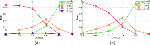
Figure 2: Confounding effects results for $D_{1}$ (a) and $D_{2}$ (b). Each marker represents the proportion of replicates (50) for which our model found 0, 1, 2 (ground truth) positives and false positives. Mind that rates for true positives sum up to 1.

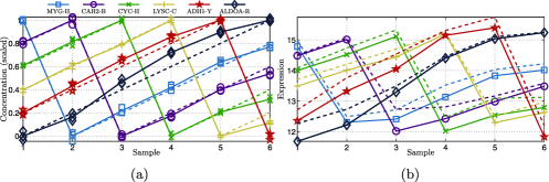
Figure 3: Spike-in data profiles. (a) Ground truth (dashed) and estimated (solid) protein profiles scaled between 0 and 1. Replicates are shown as markers and solid lines are averages across replicates. (b) Median IG expression grouped according to the labeling obtained during inference and averaged across replicates. Dashed lines correspond to original data with missing values and solid lines to data with missing values replaced by their estimates. Credible intervals were omitted for clarity.

overlap our model finds the 2 biological effects approximately 90% of the times and that such a proportion decreases to exactly zero (100% 0 true positives) as the $\tau$ approaches 1. We also see that the false positive rate is very small and that for large overlaps is always zero. As the model is currently defined, any effect that correlates with batch indicators will be treated as a batch effect, in that sense, confounded biological effects cannot—and arguably should not—be detected.

6 Spike-in data

The benchmark data set originally introduced by Mueller et al. (2007) consists of 6 samples measured in three replicates. Each sample is a mixture of six nonhuman purified proteins in different concentration levels spanning two orders of magnitude from 25 to 800 fmol. Figure 3(a) shows, in dashed lines, ground truth concentrations on a log-scale and scaled to fit in the interval $[0,1]$. The raw data containing approximately 15,900 IGs per sample was filtered down to 1841 IGs per sample after identification, annotation and exclusion of unidentified IGs with 50% missing values or with less than 10% of the maximum variance IG. Annotations are available for only 88 IGs; This is 4.7% of the set. The final data set contains 18 observations and 1841 IGs labeled with 7 protein names, ADH1-Y (12), ALDOA-R (20), CAH2-B (13), CYC-H (24), LYSC-C (9), MYG-H (10) and UKN (1753), with the number of IGs per protein in parentheses and UKN denoting unannotated IGs. The data matrix has a missingness of 30% that is more or less evenly distributed across observations. The original experiment reported by Mueller et al. (2007) only uses annotated data. Since the data set is relatively clean and all the samples were obtained in a single session, we do not expect systematic, batch effects or a meaningful covariance structure. However, we do expect high correlation due to replicates, thus, we provide $\bolds{\Phi}$ with an inverse Wishart prior with $10\times N$ degrees of freedom and scale matrix composed of 6 blocks of magnitude 0.9 and size 3 plus 0.1 times the identity matrix. Although learning the degrees of freedom and the blocks/diagonal proportions will be more principled, we did not observe substantial changes in the results from small changes in the previously mentioned values. We ran the sampler for 4000 iterations with a burin-in period of 2000.

Figure 3(a) shows the summary of the estimated latent protein profiles. Each circle represents a replicate, solid lines are averages across replicates and dashed lines represent the ground truth [see Mueller et al. (2007)]. Summaries were computed using medians and credible intervals were omitted for clarity. Summaries with credible intervals are available as the supplementary material [Henao et al. (2013c)]. Compared to the ground truth, our model does a pretty good job at capturing the underlying profiles of all 6 proteins of interest despite the large amount of missing values and unannotated IGs used.

Availability of the true protein profiles allows us to quantitatively evaluate how accurate our model is at estimating the protein profiles. We compare four different models: (i) the model for protein quantitation described in Karpievitch et al. (2009) where we have used protein concentrations as a grouping variable (Karp09) and three variants of our model, (ii) full i.i.d. latent proteins, meaning no tree structure prior; (iii) independent gamma distributions and diagonal $\bolds{\Phi}$, assumes no correlation due to replicates and (iv) inverse Wishart prior for $\bolds{\Phi}$ with scale matrix as already described. Results of model (iii) also appear in Henao et al. (2012). Although the three factor models [(ii)–(iv)] produce profiles similar to those shown in Figure 3(a), there are small differences. Table 3 indicates that in terms of mse, mae and mab, the results of the model with the inverse Wishart prior (iv) are most accurate. Although the covariance structure in the true protein profiles is not interpretable in this experiment, they are correlated, which explains why the two models with tree structure prior [(iii) and (iv)] outperform the full i.i.d. models [(i) and (ii)]. Additionally, the inverse Wishart prior in model (iv) is improved over model (iii) because the prior accounts for the sample correlation resulting from having replicates in the experiment.

=270pt Tree with $\bolds{\Phi}$ prior Measure Karp09 No tree Indep. gamma Inverse Wishart $10^{3}\times\mbox{{mse}}$ $12.370$ 2.524 1.899 1.661 $10^{2}\times\mbox{{mae}}$ $6.915$ 3.172 2.983 2.494 $10^{1}\times\mbox{{mab}}$ $3.094$ 1.443 1.252 1.213

Table 3: Performance measures for spike-in data. mse, mae and mab are mean squared error, mean absolute error and maximum absolute bias, respectively

We can use the labeling vector ${\mathbf{u}}$ to examine how unannotated isotope groups were labeled after inference. In particular, ADH1-Y went from having 12 IGs to 118, ALDOA-R from 20 to 307, CAH2-B from 13 to 240, CYC-H from 24 to 288, LYSC-C from 9 to 189 and MYG from 10 to 185. Figure 3(b) shows median IG expression grouped according to the labeling vector ${\mathbf{u}}$ and averaged across replicates to make easier comparisons against the ground truth in Figure 3(a). Dashed and solid lines correspond to data with and without missing values, respectively. For the latter, we have replaced the missing values with those estimated by our model. We see that for every protein our model estimates of missing values improve the expression average. The largest improvement is in the lower end of the expression range, precisely where the missing values are likely to be found [see Mueller et al. (2007)]. A similar picture using only the labeling from annotation does not resemble the ground truth at all. This is because the original labeling only comprises 88 IGs with a considerable amount of missing values.

7 H1N1/H3N2 viral challenge

We present now the case study based on the motivating data already described in Section 2. Here we will be using only the set of 4670 annotated IGs for which we have at least 2 IG per protein. Therefore, for this study we have $n=172$, $N_{B}=3$, $N_{F}=16$ and $N_{P}=106$. Additionally, each observation can be seen as an element of a time series of length 4, that is, $t=\{0,0.2,0.8,1\}$. If we let latent proteins have Gaussian process priors with squared exponential covariance function and assuming no sample correlation across patients, we can compute the entries of $\bolds{\Phi}$ from

$$\phi(i,j)=c_{ij}\exp\bigl{(}-\ell^{-1}d_{ij}^{2}\bigr{)}+\sigma^{2}\delta_{ij},$$

where $\ell$ is the inverse length scale, $\sigma^{2}$ the idiosyncratic noise variance, $\delta_{ij}=1$ only if $i=j$, $c_{ij}=1$ only if samples $i$ and $j$ are from the same patient, and $d_{ij}=t_{i}-t_{j}$ is the time difference between pair $\{t_{i},t_{j}\}\in\{0,0.2,0.8,1\}$. Hyperparameters $\ell$ and $\sigma^{2}$ are updated using slice sampling [Neal (2003)]. We ran the inference procedure for 5000 burn-in iterations followed by 2000 samples to compute summaries. The whole procedure takes approximately 2.5 hours in a regular desktop machine with 4 cores. Mixing was monitored using both exploratory and standard diagnostic tests. Table 4 reports the resulting

=205pt $N_{F}$ Identity Confusion Stability Unique 3 0.774 0.511 0.958 0.783

Table 4: Structural measures for viral challenge data. $N_{F}$ is selected with threshold $\rho_{j}<10^{3}$ and stability with threshold $0.6$

structural components of the model, namely, previously described: number of systematic factors, $N_{F}$, identity and confusion. We define stability as the proportion of IGs having a single value in the label vector ${\mathbf{u}}$ for at least 60% of the MCMC samples after the burn-in period. We also define unique as the proportion of latent proteins with distinct labels.

7.1 Consistency with annotation

From Table 4 we see that approximately half of the IGs ended up with a protein label different from their annotation (confusion). Possible explanations for this include systematic effects, post-translational modifications, measurement error and alignment induced mislabeling. In this example, consider the problem of aligning batches H1N1, N3N2₁ and N3N2₂. Initially, the three batches have different sets of annotation that need to be matched to create a common annotation set. We use the alignment algorithm described in Lucas et al. (2012). From the 4670 IGs included in the model, annotation was transferred from one of the batches to the other two in $64\%$ of the cases. This means that more than half of the IGs are more prone to miss-annotation due to the challenges of aligning between data sets. We found that a disproportionate percentage of peptides that retained their label from annotation after model fit are from the set of IGs with H1N1/H3N2 shared annotation. This suggests that IGs annotated simultaneously in all sets tend to be more reliable than those labeled by label transfer.

The identity of the model, on the other hand, indicates that 82 latent proteins match annotation when labeled by consensus of their IG members. The remaining latent proteins represent cases of duplicate representation of particular proteins. For example, there are 6 latent proteins associated with APOB-H (the most commonly identified protein in the data), all of them with disparate profiles. Figure 4(a) shows the composition of all latent proteins.

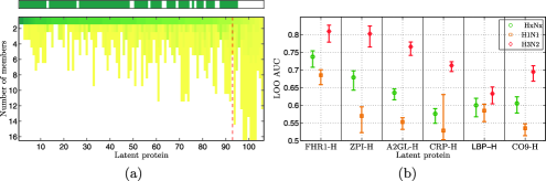
Figure 4: Protein identification and status classification. After model fitting, each latent protein contains a set of peptides, not all of which are from the same protein. (a) Number of members or protein labels per latent protein. Each column is a different latent protein. For a particular column, each row contains membership information, ordered top to bottom from most to least common for the corresponding latent protein. Color encodes member dominance, thus, dark green indicates that a given latent protein is dominated by peptides annotated by protein prophet as originating from a single protein. The red line separates latent proteins in which the leading member has a proportion less than 30%. The top bar shows in dark the 82 proteins whose posterior label matches prior information. (b) Classification accuracy presented as AUC values estimated using leave-one-out cross-validation. Markers indicate median values and error bars cover $90\%$ credible intervals.

For each latent protein (column), we tabulate and sort the labels of its IG members (rows). Darker colors represent proportions closer to 1. The first row is used to compute the consensus to determine identity. The red bar indicates whether the most frequent IG in a given latent protein is represented by less than 30% of the IGs assigned to it. The top bar shows in dark the 82 latent proteins that match their initial annotation. For most latent proteins, the most frequent IG has an important contribution and no latent protein has IGs from more than 17 different labels.

7.2 Association with phenotype and pathway analysis

We can also use latent proteins as predictors of the symptomatic vs. asymptomatic status of each observation in the data set. For this purpose, we fit individual linear discriminant classifiers for each latent protein at each MCMC draw and estimate the classification accuracy as the area under the ROC curve [AUC, Receiver Operating Characteristic, Fawcett (2006)]. Figure 4(b) shows results for the six most discriminant latent proteins: FHR1-H, ZPI-H, CRP-H, LBP-H, A2GL-H and CO9-H; It shows in particular that FHR1-H has an overall decent performance. In addition, when treating H1N1 and H3N2 as separate classification tasks, we observe that H3N2 is clearly easier to classify.

We also applied the model for protein quantitation of Karpievitch et al. (2009) using symptomatic/asymptomatic status as a grouping variable. Their model found 40 significant proteins with $q$-value threshold 0.05, which is quite a large number considering the total number of proteins in the data set is 106. In addition, almost none of these show significant association with the biological phenotype. We found only 3 proteins in common (CHLE-H, FHR1-H and HRG-H) when comparing their list to our own. For our model we used $t$-tests, $q$-values and the same 0.05 threshold to be fair with the other method. However, their list does not include ZPI-H, CRP-H, LBP-H, A2GL-H or CO9-H, all of which are strongly associated with the symptomatic versus asymptotic designation.

As described in Section 3, the prior distribution for the set of latent proteins allows us to build a binary tree representation of its elements in a hierarchical clustering fashion. When examining the resulting structure [see Henao et al. (2013a)] we found some straightforward groupings in the tree mostly corresponding to protein variants like APOC2-H and APOC3-H, CO8A-H, CO8B-H and CO8G-H, FIBG-H and FIBB-H, F13A-H and F13B-H, etc., all of them having similar profiles when looking at their estimated signatures (results not shown), in other cases, for instance, CO4(a,b)-H and APOB-H, showing great diversity in their profiles and as a result rather spread in the structure.

In an attempt to quantify whether the latent proteins and tree representation produced by our model is meaningful from a biological point of view, we performed Gene Ontology (GO) searches for the protein lists encoded by each latent protein and each tree node. In order to quantify the strength of the association between GO annotations and our protein lists, we use Bayes factors [GATHER, Chang and Nevins (2006)]. As controls we generated (i) 500 latent proteins/trees from the prior in (3) (RND) and (ii) 500 random label permutations for the latent proteins and tree produced by our model (RNP). Figure 5(a) and (b) shows separate Bayes factor

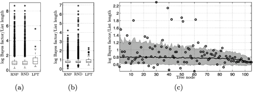
Figure 5: GO scaled log Bayes factors. (a) Latent proteins. (b) Tree nodes. (c) Bayes factors vs tree nodes for LPT (circles) and RNP (solid line). Shaded area covers 90% empirical quantiles for RNP values.

boxplots for latent proteins and tree nodes, respectively. Bayes factors have been scaled by the size of the protein list to compensate for the agglomerative mechanism of the tree structure. Differences in medians between LPT and the two controls are significant with $p$-value threshold 0.01 for both latent proteins and tree nodes. Provided that LPT and RNP have the same tree structure, we can directly compare Bayes factors at each node of the tree. Figure 5(c) shows scaled Bayes factors for each tree node of LPT (circles) and RNP (median: solid line; shade: 90% empirical quantiles). We see quite a few nodes with Bayes factors far exceeding the domain of randomly permuted protein labels. These nodes are the ones with a high level of evidence for association with the GO annotations complement activation, immune response, acute-phase response, cytolysis and response to pathogen. The node with largest Bayes factor [node 30 in Figure 5(c)] contains CRP-H and LBP-H, two of our most predictive latent proteins.

Figure 6 shows the subtree corresponding to 4 of the discriminant proteins from Figure 4(b) along with a scatter of the expression values of each latent protein. Each panel in the figure shows expression in the $y$-axis and data grouping in the $x$-axis. Data to the left-hand side of the dashed vertical line corresponds to the asymptomatic set, whereas the other side contains symptomatic observations. Each side is further grouped according to time, so points closer to the dashed vertical line are for $t=0$ (green), then $t=0.2$ (yellow), $t=0.8$ (red) and the farthest to the outside is $t=1$ (purple). The good separation of observations from times $t=\{0.8,1\}$ is the feature responsible for the classification results shown in Figure 4(b). The node above CRP-H and LBP-H in Figure 6 is node 30 in Figure 5(c).

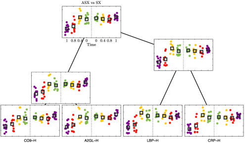
Figure 6: Discriminant subtree. This figure shows a set of three internal nodes and four leaves from the latent protein tree structure. Each node is represented as a scatter plot showing samples (dots) from the H3N2 study. The vertical dotted line separates asymptomatic (left) and symptomatic (right) samples. Samples are grouped along the $x$-axis according to time stamp: green for $t=0$ (closest to dashed line), yellow for $t=0.2$, red for $t=0.8$ and purple for $t=1$ (farthest toward the outside edge). The $y$-axis is the estimated latent/protein pathway expression. The mean for each group and time point is denoted with a square. For this group of latent proteins, the symptomatic subjects at time points $t=0.8$ and $t=1$ show clear separation.

It should be noted that the DARPA study collected samples from multiple other sources, and that there is published, publicly available gene expression data from the peripheral blood of the same patients we have examined here. That data is analyzed in Zaas et al. (2009) and a time course trajectory model is developed on a more complete version of the data in Chen et al. (2011). Together with the proteomics data included in the supplementary material [Henao et al. (2013b)], these offer interesting possibilities for future work into jointly modeling proteomics and gene expression data. We have briefly examined the correlation between protein and matched gene expression in these data sets, but find that it is generally quite low. However, an examination of the top genes discovered in Zaas et al. (2009) and the five discriminative proteins elucidated here shows a high overlap in associated pathways. We suspect that a comprehensive joint analysis of these data is complicated by the tissue of origin. Specifically, it is not clear that the proteins in blood plasma originate from peripheral blood mononuclear cells (from which there is published gene expression data). Instead, it is likely that much of the observed protein expression is due to activities in organs such as the liver or kidneys and from the endothelial lining of blood vessels.

8 Concluding remarks

We have presented a factor model specifically designed for proteomics data analysis. It successfully handles broad scale variability that is known to come from technical sources (such as batch effects and isotope group specific noise), hence enabling us to estimate latent protein profiles that better describe biological variability. Our hierarchical representation of isotope groups, latent proteins and protein pathways provides us with detailed annotation uncertainty assessment, detection of possibly inaccurately annotated isotope groups and clustering of proteins with similar expression profiles that reflect biologically related interactions. We have also shown that features of our model can be used to define predictive models based either on latent proteins or groups of latent proteins.

Appendix: MCMC inference details

We describe next the MCMC analysis mostly based on Gibbs sampling. We provide then the relevant conditional posteriors and SMC-based update details for the tree structure. To simplify notation, we use the following shorthands. Let ${\mathbf{X}}^{m}=[x_{1}^{m}\enskip\cdots\enskip x_{N_{m}}^{m}]$ and ${\mathbf{X}}=[{\mathbf{X}}^{1}\enskip\cdots\enskip{\mathbf{X}}^{N_{B}}]$, where $N_{B}$ is the number of batches, $N_{m}$ is the number of samples in batch $m$ and $N=\sum_{m=1}^{N_{B}}N_{m}$. Define ${\mathbf{1}}_{k}$ to be a $k$-dimensional row vector of ones and let $\widetilde{{\mathbf{X}}}$ be the full data set with the appropriate means subtracted off; this is $\widetilde{{\mathbf{X}}}=[{\mathbf{X}}^{1}-\bolds{\mu}^{1}{\mathbf{1}}_{N_{1}}\enskip\cdots\enskip{\mathbf{X}}^{N_{B}}-\bolds{\mu}^{N_{B}}{\mathbf{1}}_{K_{N_{B}}}]$, and ${\mathbf{Z}}=[{\mathbf{z}}_{1}\enskip\cdots\enskip{\mathbf{z}}_{N}]$ and ${\mathbf{W}}=[{\mathbf{w}}_{1}\enskip\cdots\enskip{\mathbf{w}}_{N}]$, systematic factors and latent protein matrices of sizes $N_{F}\times N$ and $N_{P}\times N$, respectively. For any matrix ${\mathbf{M}}$, define ${\mathbf{M}}_{i:}$ as its $i$th row and ${\mathbf{M}}_{:j}$ to be its $j$th column.

Noise variance

Sample each element of the diagonal of $\bolds{\Psi}$ from

$$\psi_{i}^{-1}|t_{s},t_{r}\sim\operatorname{Gamma}\biggl{(}t_{s}+\frac{N}{2},t_{r}+c\biggr{)},$$

where $t_{s}$ and $t_{r}$ are, respectively, prior shape and rate and

$$c=\tfrac{1}{2}(\widetilde{{\mathbf{X}}}_{i:}-{\mathbf{A}}_{i:}{\mathbf{Z}}-{\mathbf{B}}_{i:}{\mathbf{W}})(\widetilde{{\mathbf{X}}}_{i:}-{\mathbf{A}}_{i:}{\mathbf{Z}}-{\mathbf{B}}_{i:}{\mathbf{W}})^{\top}.$$

Batch means

Sample mean vector for batch $m$ from

$$\bolds{\mu}^{m}|t_{m},t_{p}\sim\mathcal{N}\Biggl{(}{\mathbf{C}}\Biggl{(}t_{m}t_{p}+\bolds{\Psi}^{-1}\sum_{n=1}^{N_{m}}{\mathbf{x}}_{n}^{m}-{\mathbf{A}}{\mathbf{z}}_{n}-{\mathbf{B}}{\mathbf{w}}_{n}\Biggr{)},{\mathbf{C}}\Biggr{)},$$

where ${\mathbf{C}}=(t_{p}+N_{m}\bolds{\Psi}^{-1})^{-1}$, $t_{m}$ and $t_{p}$ are prior mean and precision.

Systematic effect factors

The conditional posterior of ${\mathbf{Z}}$, using a scale mixture of Gaussian representation, can be computed independently for each element of the matrix using

$$z_{jn}|\tau_{jn}\sim\mathcal{N}\bigl{(}c_{jn}{\mathbf{A}}_{:j}^{\top}\bolds{\Psi}^{-1}\bolds{\varepsilon}_{\setminus jn},c_{jn}\bigr{)},$$

where $c_{jn}=({\mathbf{A}}_{:j}^{\top}\bolds{\Psi}^{-1}{\mathbf{A}}_{:j}+\tau_{jn}^{-1})^{-1}$ and $\bolds{\varepsilon}_{\setminus jn}={\mathbf{x}}_{n}-{\mathbf{A}}{\mathbf{z}}_{n}-{\mathbf{B}}{\mathbf{w}}_{n}-\bolds{\mu}^{m}|z_{jn}=0$. The mixing variances $\tau_{jn}$ are exponentially distributed with rate $\lambda^{2}$, hence, their resulting conditional posterior is

$$\tau_{jn}^{-1}|\lambda^{2}\sim\operatorname{IG}\biggl{(}\sqrt{\frac{\lambda^{2}}{z_{jn}}},\lambda^{2}\biggr{)},\qquad\lambda^{2}|\ell_{s},\ell_{r}\sim\operatorname{Gamma}\biggl{(}\ell_{s}+\frac{1}{2},\ell_{r}+\frac{1}{2}\sum_{j,n}\tau_{jn}\biggr{)},$$

where $\ell_{s}$ and $\ell_{r}$ are shape and rate priors, respectively. $\operatorname{IG}(\cdot|\mu,\lambda)$ is the inverse Gaussian distribution with mean $\mu$ and scale $\lambda$ [Chhikara and Folks (1989)]. Each element $a_{ij}$ from the loading matrix ${\mathbf{A}}$ is sampled from

$$a_{ij}\sim\mathcal{N}\bigl{(}c_{ij}\bolds{\varepsilon}_{\setminus ij}{\mathbf{Z}}_{l:}^{\top},c_{ij}\psi_{i}\bigr{)},$$

where $c_{ij}=({\mathbf{Z}}_{j:}{\mathbf{Z}}_{j:}^{\top}+\psi_{i}\rho_{j})^{-1}$ and $\bolds{\varepsilon}_{\setminus ij}=\widetilde{{\mathbf{X}}}_{i:}-{\mathbf{A}}_{i:}{\mathbf{Z}}-{\mathbf{B}}_{i:}{\mathbf{W}}|a_{ij}=0$. Then, column-wise precisions for ${\mathbf{A}}$ are drawn from

$$\rho_{j}|r_{s},r_{r}\sim\operatorname{Gamma}\biggl{(}r_{s}+\frac{p}{2},r_{r}+\sum_{i}a_{ij}^{2}\biggr{)},$$

where $r_{s}$ and $r_{r}$ are prior shape and rate, respectively.

Protein profiles

The conditional posterior for latent proteins ${\mathbf{W}}$ can be updated from

$${\mathbf{W}}_{k:}|{\mathbf{v}}_{k}\sim\mathcal{N}\bigl{(}{\mathbf{C}}{\mathbf{B}}_{:k}^{\top}\bolds{\Psi}^{-1}(\widetilde{{\mathbf{X}}}-{\mathbf{A}}{\mathbf{Z}})+{\mathbf{C}}{\mathbf{S}}_{k}^{-1}{\mathbf{m}}_{k},{\mathbf{C}}\bigr{)},$$

where ${\mathbf{C}}=({\mathbf{B}}_{:k}^{\top}\bolds{\Psi}^{-1}{\mathbf{B}}_{:k}+{\mathbf{S}}_{k}^{-1})^{-1}$, with ${\mathbf{m}}_{k}$ and ${\mathbf{S}}_{k}$ being mean and covariance of the parent profile ${\mathbf{v}}_{k}$ of ${\mathbf{W}}_{k:}$. Note that $b_{ik}=0$ for all isotope groups not assumed to be part of this protein, and that these will not contribute to the update distribution for ${\mathbf{W}}_{k:}$. Besides,

$$b_{ik}|b_{ik}\neq 0\sim\mathcal{N}_{+}\bigl{(}c(\widetilde{{\mathbf{X}}}_{i:}-{\mathbf{A}}_{i:}{\mathbf{Z}}){\mathbf{W}}_{k:}^{\top},c\psi_{i}\bigr{)},$$

where $c=({\mathbf{W}}_{k:}{\mathbf{W}}_{k:}^{\top}+\psi_{i})^{-1}$ and $\mathcal{N}_{+}(\cdot)$ is the Gaussian distribution truncated below zero. Now we can sample IG-latent protein assignments from

$$\displaystyle u_{i}|\alpha,\bolds{\kappa},t_{s},t_{r}\sim\operatorname{Discrete}({\mathbf{v}}_{i}),$$

$$\displaystyle v_{k}\propto(\alpha+n_{k})c^{-{1}/{2}}\bigl{(}t_{r}+\tfrac{1}{2}\widetilde{{\mathbf{X}}}_{i:}\widetilde{{\mathbf{X}}}_{i:}^{\top}-\tfrac{1}{2}c^{-1}\widetilde{{\mathbf{X}}}_{i:}{\mathbf{W}}_{k:}^{\top}{\mathbf{W}}_{k:}\widetilde{{\mathbf{X}}}_{i:}^{\top}\bigr{)}^{-(t_{s}+{N}/{2})},$$

where $n_{k}$ is the number of nonzero entries in column $k$ of ${\mathbf{B}}$, $c={\mathbf{W}}_{k:}{\mathbf{W}}_{k:}^{\top}$ and $v_{k}$ is the $k$th element of ${\mathbf{v}}_{i}$.

Protein pathway expression and tree structure

We sample the tree structure components ${\mathbf{t}}$, $\bolds{\pi}$ and $\bolds{\Phi}$, and the means and covariances of each internal node of the tree, ${\mathbf{m}}_{k}$ and ${\mathbf{S}}_{k}$, respectively, using the SMC sampler described in Henao and Lucas (2012). In particular, $\{{\mathbf{t}},\bolds{\pi}\}$ are obtained for a number $M$ of particles, as a leaves to root SMC pass, together with partial updates of the node parameters $\{{\mathbf{m}}_{k},{\mathbf{S}}_{k}\}$. Next we use the particle’s weights to sample a single configuration. The procedure is completed by resampling the hyperparameters of the covariance function and by completing the updates of the node parameters using the selected configuration, the latter as a root to leaves pass.

Missing values

For each missing value $x_{in}^{m}$ corresponding to isotope group $i$, sample $n$ and batch $m$, we simply use independent standardized Gaussian prior distributions.

Initialization

We start the model from maximum likelihood estimates of the less critical quantities, that is, batch means $\{\bolds{\mu}^{m}\}_{m=1}^{N_{B}}$ and noise variances $\bolds{\Psi}$. Systematic factors ${\mathbf{Z}}$ and latent proteins ${\mathbf{W}}$ are initialized using standardized Gaussian distributions. The loading matrices ${\mathbf{A}}$ and ${\mathbf{B}}$ (nonzero elements only) were set to ordinary least squares estimates based upon already set ${\mathbf{Z}}$ and ${\mathbf{W}}$, respectively. The vector of associations ${\mathbf{u}}$ was set with the information obtained from annotation about IG-protein assignments.

References

- Adams, Ghahramani and Jordan (2010) {bincollection}[author] \bauthor\bsnmAdams, \bfnmR. P.\binitsR. P., \bauthor\bsnmGhahramani, \bfnmZ.\binitsZ. and \bauthor\bsnmJordan, \bfnmM. I.\binitsM. I. (\byear2010). \btitleTree-structured stick breaking for hierarchical data. In \bbooktitleAdvances in Neural Information Processing Systems 23 (\beditor\bfnmJ.\binitsJ. \bsnmLafferty, \beditor\bfnmC. K. I.\binitsC. K. I. \bsnmWilliams, \beditor\bfnmJ.\binitsJ. \bsnmShawe-Taylor, \beditor\bfnmR. S.\binitsR. S. \bsnmZemel and \beditor\bfnmA.\binitsA. \bsnmCulotta, eds.) \bpages19–27. \bpublisherMIT Press, \blocationCambridge, MA. \bptokimsref \endbibitem
- Aebersold and Mann (2003) {barticle}[pbm] \bauthor\bsnmAebersold, \bfnmRuedi\binitsR. and \bauthor\bsnmMann, \bfnmMatthias\binitsM. (\byear2003). \btitleMass spectrometry-based proteomics. \bjournalNature \bvolume422 \bpages198–207. \biddoi=10.1038/nature01511, issn=0028-0836, pii=nature01511, pmid=12634793 \bptokimsref \endbibitem
- Andrews and Mallows (1974) {barticle}[mr] \bauthor\bsnmAndrews, \bfnmD. F.\binitsD. F. and \bauthor\bsnmMallows, \bfnmC. L.\binitsC. L. (\byear1974). \btitleScale mixtures of normal distributions. \bjournalJ. R. Stat. Soc. Ser. B Stat. Methodol. \bvolume36 \bpages99–102. \bidissn=0035-9246, mr=0359122 \bptokimsref \endbibitem
- Baggerly et al. (2004) {barticle}[pbm] \bauthor\bsnmBaggerly, \bfnmK. A.\binitsK. A., \bauthor\bsnmEdmonson, \bfnmS. R.\binitsS. R., \bauthor\bsnmMorris, \bfnmJ. S.\binitsJ. S. and \bauthor\bsnmCoombes, \bfnmK. R.\binitsK. R. (\byear2004). \btitleHigh-resolution serum proteomic patterns for ovarian cancer detection. \bjournalEndocr. Relat. Cancer \bvolume11 \bpages583–584. \bptokimsref \endbibitem
- Carvalho et al. (2008) {barticle}[mr] \bauthor\bsnmCarvalho, \bfnmCarlos M.\binitsC. M., \bauthor\bsnmChang, \bfnmJeffrey\binitsJ., \bauthor\bsnmLucas, \bfnmJoseph E.\binitsJ. E., \bauthor\bsnmNevins, \bfnmJoseph R.\binitsJ. R., \bauthor\bsnmWang, \bfnmQuanli\binitsQ. and \bauthor\bsnmWest, \bfnmMike\binitsM. (\byear2008). \btitleHigh-dimensional sparse factor modeling: Applications in gene expression genomics. \bjournalJ. Amer. Statist. Assoc. \bvolume103 \bpages1438–1456. \biddoi=10.1198/016214508000000869, issn=0162-1459, mr=2655722 \bptokimsref \endbibitem
- Chang and Nevins (2006) {barticle}[pbm] \bauthor\bsnmChang, \bfnmJeffrey T.\binitsJ. T. and \bauthor\bsnmNevins, \bfnmJoseph R.\binitsJ. R. (\byear2006). \btitleGATHER: A systems approach to interpreting genomic signatures. \bjournalBioinformatics \bvolume22 \bpages2926–2933. \biddoi=10.1093/bioinformatics/btl483, issn=1367-4811, pii=btl483, pmid=17000751 \bptokimsref \endbibitem
- Chen et al. (2011) {barticle}[mr] \bauthor\bsnmChen, \bfnmMinhua\binitsM., \bauthor\bsnmZaas, \bfnmAimee\binitsA., \bauthor\bsnmWoods, \bfnmChristopher\binitsC., \bauthor\bsnmGinsburg, \bfnmGeoffrey S.\binitsG. S., \bauthor\bsnmLucas, \bfnmJoseph\binitsJ., \bauthor\bsnmDunson, \bfnmDavid\binitsD. and \bauthor\bsnmCarin, \bfnmLawrence\binitsL. (\byear2011). \btitlePredicting viral infection from high-dimensional biomarker trajectories. \bjournalJ. Amer. Statist. Assoc. \bvolume106 \bpages1259–1279. \biddoi=10.1198/jasa.2011.ap10611, issn=0162-1459, mr=2896834 \bptokimsref \endbibitem
- Chhikara and Folks (1989) {bbook}[author] \bauthor\bsnmChhikara, \bfnmR. S.\binitsR. S. and \bauthor\bsnmFolks, \bfnmL.\binitsL. (\byear1989). \btitleThe Inverse Gaussian Distribution: Theory, Methodology, and Applications. \bpublisherDekker, \blocationNew York. \bptokimsref \endbibitem
- Clough et al. (2009) {barticle}[pbm] \bauthor\bsnmClough, \bfnmTimothy\binitsT., \bauthor\bsnmKey, \bfnmMelissa\binitsM., \bauthor\bsnmOtt, \bfnmIlka\binitsI., \bauthor\bsnmRagg, \bfnmSusanne\binitsS., \bauthor\bsnmSchadow, \bfnmGunther\binitsG. and \bauthor\bsnmVitek, \bfnmOlga\binitsO. (\byear2009). \btitleProtein quantification in label-free LC–MS experiments. \bjournalJ. Proteome Res. \bvolume8 \bpages5275–5284. \biddoi=10.1021/pr900610q, issn=1535-3907, pmid=19891509 \bptokimsref \endbibitem
- Daly et al. (2008) {barticle}[author] \bauthor\bsnmDaly, \bfnmD. S.\binitsD. S., \bauthor\bsnmAnderson, \bfnmK. K.\binitsK. K., \bauthor\bsnmPanisko, \bfnmE. A.\binitsE. A., \bauthor\bsnmPurvine, \bfnmS. O.\binitsS. O., \bauthor\bsnmFang, \bfnmR.\binitsR., \bauthor\bsnmMonroe, \bfnmM. E.\binitsM. E. and \bauthor\bsnmBaker, \bfnmS. E.\binitsS. E. (\byear2008). \btitleMixed-effects statistical model for comparative LC–MS proteomics studies. \bjournalProteomics Research \bvolume7 \bpages1209–1217. \bptokimsref \endbibitem
- Escobar and West (1995) {barticle}[mr] \bauthor\bsnmEscobar, \bfnmMichael D.\binitsM. D. and \bauthor\bsnmWest, \bfnmMike\binitsM. (\byear1995). \btitleBayesian density estimation and inference using mixtures. \bjournalJ. Amer. Statist. Assoc. \bvolume90 \bpages577–588. \bidissn=0162-1459, mr=1340510 \bptokimsref \endbibitem
- Fawcett (2006) {barticle}[author] \bauthor\bsnmFawcett, \bfnmT.\binitsT. (\byear2006). \btitleAn introduction to ROC analysis. \bjournalPattern Recognition Letters \bvolume27 \bpages861–874. \bptokimsref \endbibitem
- Henao and Lucas (2012) {bmisc}[author] \bauthor\bsnmHenao, \bfnmR.\binitsR. and \bauthor\bsnmLucas, \bfnmJ. E.\binitsJ. E. (\byear2012). \bhowpublishedEfficient hierarchical clustering for continuous data. Technical report, Institute for genome Science and Policy, Duke Univ. Available at arXiv:\arxivurl1204.4708. \bptokimsref \endbibitem
- Henao and Winther (2011) {barticle}[mr] \bauthor\bsnmHenao, \bfnmRicardo\binitsR. and \bauthor\bsnmWinther, \bfnmOle\binitsO. (\byear2011). \btitleSparse linear identifiable multivariate modeling. \bjournalJ. Mach. Learn. Res. \bvolume12 \bpages863–905. \bidissn=1532-4435, mr=2786913 \bptokimsref \endbibitem
- Henao et al. (2012) {binproceedings}[author] \bauthor\bsnmHenao, \bfnmR.\binitsR., \bauthor\bsnmThompson, \bfnmJ. W.\binitsJ. W., \bauthor\bsnmMoseley, \bfnmM. A.\binitsM. A., \bauthor\bsnmGinsburg, \bfnmG. S.\binitsG. S., \bauthor\bsnmCarin, \bfnmL.\binitsL. and \bauthor\bsnmLucas, \bfnmJ. E.\binitsJ. E. (\byear2012). \btitleHierarchical factor modeling of proteomics data. In \bbooktitleIEEE 2nd International Conference on Computational Advances in Bio and Medical Sciences (ICCABS), 2012. \bptokimsref \endbibitem
- Henao et al. (2013a) {bmisc}[author] \bauthor\bsnmHenao, \bfnmR.\binitsR., \bauthor\bsnmThompson, \bfnmJ. W.\binitsJ. W., \bauthor\bsnmMoseley, \bfnmM. A.\binitsM. A., \bauthor\bsnmGinsburg, \bfnmG. S.\binitsG. S., \bauthor\bsnmCarin, \bfnmL.\binitsL. and \bauthor\bsnmLucas, \bfnmJ. E.\binitsJ. E. (\byear2013a). \bhowpublishedSupplement to “Latent protein trees.” DOI:\doiurl10.1214/13-AOAS639SUPPA. \bptokimsref \endbibitem
- Henao et al. (2013b) {bmisc}[author] \bauthor\bsnmHenao, \bfnmR.\binitsR., \bauthor\bsnmThompson, \bfnmJ. W.\binitsJ. W., \bauthor\bsnmMoseley, \bfnmM. A.\binitsM. A., \bauthor\bsnmGinsburg, \bfnmG. S.\binitsG. S., \bauthor\bsnmCarin, \bfnmL.\binitsL. and \bauthor\bsnmLucas, \bfnmJ. E.\binitsJ. E. (\byear2013b). \bhowpublishedSupplement to “Latent protein trees.” DOI:\doiurl10.1214/13-AOAS639SUPPB. \bptokimsref \endbibitem
- Henao et al. (2013c) {bmisc}[author] \bauthor\bsnmHenao, \bfnmR.\binitsR., \bauthor\bsnmThompson, \bfnmJ. W.\binitsJ. W., \bauthor\bsnmMoseley, \bfnmM. A.\binitsM. A., \bauthor\bsnmGinsburg, \bfnmG. S.\binitsG. S., \bauthor\bsnmCarin, \bfnmL.\binitsL. and \bauthor\bsnmLucas, \bfnmJ. E.\binitsJ. E. (\byear2013c). \bhowpublishedSupplement to “Latent protein trees.” DOI:\doiurl10.1214/13-AOAS639SUPPC. \bptokimsref \endbibitem
- Kagan, Linnik and Rao (1973) {bbook}[mr] \bauthor\bsnmKagan, \bfnmA. M.\binitsA. M., \bauthor\bsnmLinnik, \bfnmYu. V.\binitsY. V. and \bauthor\bsnmRao, \bfnmC. Radhakrishna\binitsC. R. (\byear1973). \btitleCharacterization Problems in Mathematical Statistics. \bpublisherWiley, \blocationNew York. \bidmr=0346969 \bptokimsref \endbibitem
- Karpievitch et al. (2009) {barticle}[author] \bauthor\bsnmKarpievitch, \bfnmY. V.\binitsY. V., \bauthor\bsnmStanley, \bfnmJ.\binitsJ., \bauthor\bsnmTaverner, \bfnmT.\binitsT., \bauthor\bsnmHuang, \bfnmJ.\binitsJ., \bauthor\bsnmAdkins, \bfnmJ. N.\binitsJ. N., \bauthor\bsnmAnsong, \bfnmC.\binitsC., \bauthor\bsnmHeffron, \bfnmF.\binitsF., \bauthor\bsnmMetz, \bfnmT. O.\binitsT. O., \bauthor\bsnmQian, \bfnmW. J.\binitsW. J., \bauthor\bsnmYoon, \bfnmH.\binitsH., \bauthor\bsnmSmith, \bfnmR. D.\binitsR. D. and \bauthor\bsnmDabney, \bfnmA. R.\binitsA. R. (\byear2009). \btitleA statistical framework for protein quantitation in bottom-up MS-based proteomics. \bjournalBioinformatics \bvolume25 \bpages2028–2034. \bptokimsref \endbibitem
- Keller et al. (2002) {barticle}[author] \bauthor\bsnmKeller, \bfnmA.\binitsA., \bauthor\bsnmNesvizhskii, \bfnmA. I.\binitsA. I., \bauthor\bsnmKolker, \bfnmE.\binitsE. and \bauthor\bsnmAebersold, \bfnmR.\binitsR. (\byear2002). \btitleEmpirical statistical model to estimate the accuracy of peptide identifications made by MS/MS and database search. \bjournalAnalytica Chemistry \bvolume74 \bpages5384–5392. \bptokimsref \endbibitem
- Kingman (1982a) {barticle}[mr] \bauthor\bsnmKingman, \bfnmJ. F. C.\binitsJ. F. C. (\byear1982a). \btitleThe coalescent. \bjournalStochastic Process. Appl. \bvolume13 \bpages235–248. \biddoi=10.1016/0304-4149(82)90011-4, issn=0304-4149, mr=0671034 \bptokimsref \endbibitem
- Kingman (1982b) {barticle}[mr] \bauthor\bsnmKingman, \bfnmJ. F. C.\binitsJ. F. C. (\byear1982b). \btitleOn the genealogy of large populations. Essays in statistical science. \bjournalJ. Appl. Probab. \bvolume19 \bpages27–43. \bidissn=0170-9739, mr=0633178 \bptokimsref \endbibitem
- Leek et al. (2010) {barticle}[pbm] \bauthor\bsnmLeek, \bfnmJeffrey T.\binitsJ. T., \bauthor\bsnmScharpf, \bfnmRobert B.\binitsR. B., \bauthor\bsnmBravo, \bfnmHéctor Corrada\binitsH. C., \bauthor\bsnmSimcha, \bfnmDavid\binitsD., \bauthor\bsnmLangmead, \bfnmBenjamin\binitsB., \bauthor\bsnmJohnson, \bfnmW. Evan\binitsW. E., \bauthor\bsnmGeman, \bfnmDonald\binitsD., \bauthor\bsnmBaggerly, \bfnmKeith\binitsK. and \bauthor\bsnmIrizarry, \bfnmRafael A.\binitsR. A. (\byear2010). \btitleTackling the widespread and critical impact of batch effects in high-throughput data. \bjournalNat. Rev. Genet. \bvolume11 \bpages733–739. \biddoi=10.1038/nrg2825, issn=1471-0064, pii=nrg2825, pmid=20838408 \bptokimsref \endbibitem
- Lucas et al. (2012) {barticle}[author] \bauthor\bsnmLucas, \bfnmJ. E.\binitsJ. E., \bauthor\bsnmThompson, \bfnmJ. W.\binitsJ. W., \bauthor\bsnmDubois, \bfnmL. G.\binitsL. G., \bauthor\bsnmMcCarthy, \bfnmJ.\binitsJ., \bauthor\bsnmTillman, \bfnmH.\binitsH., \bauthor\bsnmThompson, \bfnmA.\binitsA., \bauthor\bsnmShire, \bfnmN.\binitsN., \bauthor\bsnmHendrickson, \bfnmR.\binitsR., \bauthor\bsnmDieguez, \bfnmF.\binitsF., \bauthor\bsnmGoldman, \bfnmP.\binitsP., \bauthor\bsnmSchwartz, \bfnmK.\binitsK., \bauthor\bsnmPatel, \bfnmK.\binitsK., \bauthor\bsnmMcHutchison, \bfnmJ.\binitsJ. and \bauthor\bsnmMoseley, \bfnmM. A.\binitsM. A. (\byear2012). \btitleMetaprotein expression modeling for label-free quantitative proteomics. \bjournalBMC Bioinformatics \bvolume3 \bpages1–18. \bptokimsref \endbibitem
- Mueller et al. (2007) {barticle}[pbm] \bauthor\bsnmMueller, \bfnmLukas N.\binitsL. N., \bauthor\bsnmRinner, \bfnmOliver\binitsO., \bauthor\bsnmSchmidt, \bfnmAlexander\binitsA., \bauthor\bsnmLetarte, \bfnmSimon\binitsS., \bauthor\bsnmBodenmiller, \bfnmBernd\binitsB., \bauthor\bsnmBrusniak, \bfnmMi-Youn\binitsM.-Y., \bauthor\bsnmVitek, \bfnmOlga\binitsO., \bauthor\bsnmAebersold, \bfnmRuedi\binitsR. and \bauthor\bsnmMüller, \bfnmMarkus\binitsM. (\byear2007). \btitleSuperHirn—A novel tool for high resolution LC–MS-based peptide/protein profiling. \bjournalProteomics \bvolume7 \bpages3470–3480. \biddoi=10.1002/pmic.200700057, issn=1615-9853, pmid=17726677 \bptokimsref \endbibitem
- Neal (1996) {bbook}[author] \bauthor\bsnmNeal, \bfnmR. M.\binitsR. M. (\byear1996). \btitleBayesian Learning for Neural Networks. \bseriesLecture Notes in Statistics \bvolume118. \bpublisherSpringer, \blocationNew York. \bptokimsref \endbibitem
- Neal (2003) {barticle}[mr] \bauthor\bsnmNeal, \bfnmRadford M.\binitsR. M. (\byear2003). \btitleSlice sampling. \bjournalAnn. Statist. \bvolume31 \bpages705–741. \bptokimsref \endbibitem
- Nesvizhskii et al. (2003) {barticle}[pbm] \bauthor\bsnmNesvizhskii, \bfnmAlexey I.\binitsA. I., \bauthor\bsnmKeller, \bfnmAndrew\binitsA., \bauthor\bsnmKolker, \bfnmEugene\binitsE. and \bauthor\bsnmAebersold, \bfnmRuedi\binitsR. (\byear2003). \btitleA statistical model for identifying proteins by tandem mass spectrometry. \bjournalAnal. Chem. \bvolume75 \bpages4646–4658. \bidissn=0003-2700, pmid=14632076 \bptokimsref \endbibitem
- Perkins et al. (1999) {barticle}[author] \bauthor\bsnmPerkins, \bfnmD. N.\binitsD. N., \bauthor\bsnmPappin, \bfnmD. J. C\binitsD. J. C., \bauthor\bsnmCreasy, \bfnmD. M.\binitsD. M. and \bauthor\bsnmCottrell, \bfnmJ. S.\binitsJ. S. (\byear1999). \btitleProbability-based protein identification by searching sequence databases using mass spectrometry data. \bjournalElectrophoresis \bvolume20 \bpages3551–3567. \bptokimsref \endbibitem
- Petricoin et al. (2002) {barticle}[pbm] \bauthor\bsnmPetricoin, \bfnmEmanuel F.\binitsE. F., \bauthor\bsnmArdekani, \bfnmAli M.\binitsA. M., \bauthor\bsnmHitt, \bfnmBen A.\binitsB. A., \bauthor\bsnmLevine, \bfnmPeter J.\binitsP. J., \bauthor\bsnmFusaro, \bfnmVincent A.\binitsV. A., \bauthor\bsnmSteinberg, \bfnmSeth M.\binitsS. M., \bauthor\bsnmMills, \bfnmGordon B.\binitsG. B., \bauthor\bsnmSimone, \bfnmCharles\binitsC., \bauthor\bsnmFishman, \bfnmDavid A.\binitsD. A., \bauthor\bsnmKohn, \bfnmElise C.\binitsE. C. and \bauthor\bsnmLiotta, \bfnmLance A.\binitsL. A. (\byear2002). \btitleUse of proteomic patterns in serum to identify ovarian cancer. \bjournalThe Lancet \bvolume359 \bpages572–577. \biddoi=10.1016/S0140-6736(02)07746-2, issn=0140-6736, pii=S0140-6736(02)07746-2, pmid=11867112 \bptokimsref \endbibitem
- Ping (2009) {barticle}[pbm] \bauthor\bsnmPing, \bfnmPeipei\binitsP. (\byear2009). \btitleGetting to the heart of proteomics. \bjournalN. Engl. J. Med. \bvolume360 \bpages532–534. \biddoi=10.1056/NEJMcibr0808487, issn=1533-4406, mid=NIHMS107158, pii=360/5/532, pmcid=2692588, pmid=19179323 \bptokimsref \endbibitem
- Polpitiya et al. (2008) {barticle}[author] \bauthor\bsnmPolpitiya, \bfnmA. D.\binitsA. D., \bauthor\bsnmQian, \bfnmW. J.\binitsW. J., \bauthor\bsnmJaitly, \bfnmN.\binitsN., \bauthor\bsnmPetyuk, \bfnmV. A.\binitsV. A., \bauthor\bsnmAdkins, \bfnmJ. N.\binitsJ. N., \bauthor\bsnmII, \bfnmD. G. Camp\binitsD. G. C., \bauthor\bsnmAnderson, \bfnmG. A.\binitsG. A. and \bauthor\bsnmSmith, \bfnmR. D.\binitsR. D. (\byear2008). \btitleDAnTE: A statistical tool for quantitative analysis of -omics data. \bjournalBioinformatics \bvolume24 \bpages1556–1558. \bptokimsref \endbibitem
- Service (2008) {barticle}[pbm] \bauthor\bsnmService, \bfnmRobert F.\binitsR. F. (\byear2008). \btitleProteomics ponders prime time. \bjournalScience \bvolume321 \bpages1758–1761. \biddoi=10.1126/science.321.5897.1758, issn=1095-9203, pii=321/5897/1758, pmid=18818332 \bptokimsref \endbibitem
- Teh, Daume III and Roy (2008) {bincollection}[author] \bauthor\bsnmTeh, \bfnmY. W.\binitsY. W., \bauthor\bsnmDaume III, \bfnmH.\binitsH. and \bauthor\bsnmRoy, \bfnmD.\binitsD. (\byear2008). \btitleBayesian agglomerative clustering with coalescents. In \bbooktitleAdvances in Neural Information Processing Systems 20 (\beditor\bfnmJ. C.\binitsJ. C. \bsnmPlatt, \beditor\bfnmD.\binitsD. \bsnmKoller, \beditor\bfnmY.\binitsY. \bsnmSinger and \beditor\bfnmS. T.\binitsS. T. \bsnmRoweis, eds.) \bpages1473–1480. \bpublisherMIT Press, \blocationCambridge, MA. \bptokimsref \endbibitem
- Zaas et al. (2009) {barticle}[author] \bauthor\bsnmZaas, \bfnmA. K.\binitsA. K., \bauthor\bsnmChen, \bfnmM.\binitsM., \bauthor\bsnmVarkey, \bfnmJ.\binitsJ., \bauthor\bsnmVeldman, \bfnmT.\binitsT., \bauthor\bsnmHero, \bfnmA. O.\binitsA. O., \bauthor\bsnmLucas, \bfnmJ.\binitsJ., \bauthor\bsnmHuang, \bfnmY.\binitsY., \bauthor\bsnmTurner, \bfnmR.\binitsR., \bauthor\bsnmGilbert, \bfnmA.\binitsA., \bauthor\bsnmLambkin-Williams, \bfnmR.\binitsR., \bauthor\bsnmØien, \bfnmN. C.\binitsN. C., \bauthor\bsnmNicholson, \bfnmB.\binitsB., \bauthor\bsnmKingsmore, \bfnmS.\binitsS., \bauthor\bsnmCarin, \bfnmL.\binitsL., \bauthor\bsnmWoods, \bfnmC. W.\binitsC. W. and \bauthor\bsnmGinsburg, \bfnmG. S.\binitsG. S. (\byear2009). \btitleGene expression signatures diagnose influenza and other symptomatic respiratory viral infections in humans. \bjournalCell \bvolume6 \bpages207–217. \bptokimsref \endbibitem
- Zhang and Chan (2005) {barticle}[author] \bauthor\bsnmZhang, \bfnmZ.\binitsZ. and \bauthor\bsnmChan, \bfnmD. W.\binitsD. W. (\byear2005). \btitleCancer proteomics: In pursuit of “true” biomarker discovery. \bjournalCancer Epidemiology Biomarkers & Prevention \bvolume14 \bpages2283–2286. \bptokimsref \endbibitem