A distance scale of planetary nebulae based on mid-infrared data

Abstract

Some of the most successful statistical methods for obtaining distances of planetary nebulae (PNe) are based on their apparent sizes and radio emission intensities. These methods have the advantage of being “extinction-free” and are especially suited to be applied to PNe situated at large distances. A similar method, based on the mid-infrared (MIR) emission of PNe, would have the advantage of being applicable to the large databases created after the various all-sky or Galactic plane infrared surveys, such as IRAS, MSX, ISOGAL, GLIMPSE, etc. In this work we propose a statistical method to calculate the distance of PNe based on the apparent nebular radius and the MIR flux densities. We show that the specific intensity between 8 and 21 micron is proportional to the brightness temperature $T_{b}$ at 5 GHz. Using MIR flux densities at 8, 12, 15 and 21 microns from the MSX survey, we calibrate the distance scale with a statistical method by Stanghellini et al. 2008 (SSV). The database used in the calibration consisted of 67 Galactic PNe with MSX counterparts and distances determined by SSV. We apply the method to a sample of PNe detected at 8 microns in the GLIMPSE infrared survey, and determine the distance of a sample of PNe located along the Galactic plane and bulge.

1 Introduction

The problem of determining the distances of Planetary Nebulae (PNe) has long been considered a cumbersome issue because of the numerous complexities related to the evolution of these objects. Classical approaches to this problem include trigonometric parallaxes (Harris et al. 1997), the expansion method (Terzian 1997), spectroscopic distances (Méndez et al. 1988), etc. PNe nuclei are far from being considered as “standard candles” since they evolve differently according to their masses, a parameter that in most cases is not easily determined. When the central star is not visible, alternative methods based on properties of the nebula itself are required. These methods are often treated as “statistical”, and are based on nebular properties such as the ionized mass (Shklovsky 1956), the evolution of the nebular optical depth with time (Kwok 1985, Marten & Schoenberner 1991), the electron density (Barlow 1987), etc.

The first statistical method proposed in the literature, attributed to Shklovsky (1956), is based on the assumption that the nebular ionized mass is an invariant. Although this hypothesis has some limitations (Maciel & Pottasch 1980), the method represents a milestone to the distance problem, and was used as a first step to calibrate other similar methods that followed (Daub 1982, Cahn, Kaler & Stanghellini 1992). Methods based on radio quantities have several advantages over those derived from visual: the interstellar extinction does not play a critical role, even in the cases where the PNe are severely affected by interstellar extinction; radio fluxes are available for a large number of objects, etc. In addition to that, in the last three decades the increasing number of observations carried out at high spatial resolution, such as the VLA (Zijlstra et al. 1989), has largely improved our knowledge of young, compact PNe. On the other hand, comparisons among some of these “radio” distance scales (Zhang 1995; Phillips 2002, 2004) reveal that they often exhibit significant biases, showing that the problem is still an open issue.

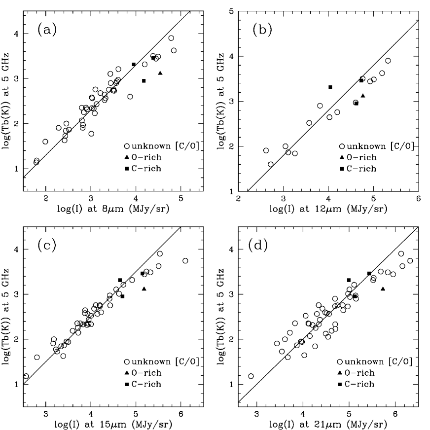
Figure 1: Brightness temperature at 5 GHz as a function of the specific intensity at 8 (a), 12 (b), 15 (c) and 21 (d) $\mu$m. The straight line represents the best fit with slope $\partial\log T_{b}/\partial\log I_{\lambda}=1$. Open circles represent PNe without [C/O] data; filled triangles depict O-rich PNe, classified according to their mid-infrared spectra; filled squares represent PNe with carbonaceous features in their spectra. PNe evolve from the top-right to the bottom-left corner of this figure: the radio emission becomes optically thinner whilst the infrared intensity decreases with time.

Mid and far-infrared data constitute an interesting alternative to approach the distance problem, because PNe are generally strong infrared sources and their emission in this band is little affected by the interstellar extinction. These two characteristics allow the detection of PNe severely obscured by dust, such as PNe hidden in the galactic plane, for example. A relationship between the nebular emission at infrared and radio wavelengths was established by Zhang & Kwok (1993), who studied the correlation between the IRAS specific intensity at 60 $\mu$m ($I_{60}$) and the brightness temperature ($T_{\rm b}$) at 5 GHz. These two distance-independent parameters can be correlated with the nebular size to compose a new distance scale. Unfortunately IRAS fluxes suffer from poor spatial resolution ($\sim 1$′) and the severe crowdness at low Galactic latitudes, limitations that were partially overcame by the MSX survey (Egan et al. 1997, 1999), thanks to its better spatial resolution ($\sim 18$″). MSX covered the Galactic plane between $|b|<5^{o}$ in 4 photometric bands, centred at 8, 12, 15 and 21 $\mu$m. Another milestone infrared survey was ISOGAL (Omont et al. 2003), a part of the ISO mission designed to obtain mid-infrared images of the Galactic bulge and specific regions of the Galactic plane with spatial resolution better than 6″ mainly at 7 and 15 $\mu$m. Although its sensitivity was almost two orders of magnitude deeper than IRAS and MSX, ISOGAL suffered from its small sky coverage, limited to only $\sim 16$ square degrees. Nevertheless, the total number of detections, including point and extended sources, amounts to $\sim 10^{5}$ objects. More recently, the Galactic plane and bulge were surveyed by GLIMPSE (Galactic Legacy Infrared Mid-Plane Survey Extraordinaire, Fazio et al. 2004), a project developed as a part of the “Spitzer” mission. GLIMPSE was restricted to $|l|<65^{o}$ and carried out with the infrared camera “IRAC”, which obtained images simultaneously in four mid-infrared bands, centred at 3.6, 4.5, 5.8 and 8.0 $\mu$m and with spatial resolution better than 2″. These surveys contain hundreds of infrared counterparts of PNe that can be used as an efficient tool to derive the distance of PNe severely affected by interstellar extinction, especially those situated along the Galactic plane.

Table 1: The MSX bands and the coefficients of equation 4.

Band	${\lambda}_{\mathrm{i}so}$($\mu$m)	aλ	bλ	cλ	N
A	8.28	$-$0.1736	$-$0.3899	+0.7960	59
C	12.13	$-$0.2728	$-$0.2551	+0.8527	15
D	14.65	$-$0.2491	$-$0.3291	+0.9217	56
E	21.34	$-$0.2382	$-$0.3242	+1.0342	52

The main purpose of the present study is to derive a new distance scale based on a minimal set of data: mid-infrared intensities and the angular size. Although the present calibration is based on MSX flux densities (at 8, 12, 15 and 21 $\mu$m), it can be extended to other existing data extracted from past (such as IRAS, ISOGAL, GLIMPSE) or future surveys carried out at similar wavelengths.

This paper is organized as follows: Sect. 2 contains a general discussion of the radio and infrared emission of PNe and the definition of basic concepts used in the following sections; Sect. 3 presents the formulation of the method and its calibration; Sect. 4 is devoted to show the results, including an application of the method to PNe detected by Spitzer; our conclusions are presented in Sect. 5.

2 The radio and infrared emission of planetary nebulae

Since the formation of a planetary nebula succeeds the Asymptotic Giant Branch (AGB), much of the circumstellar dust formed during this latter phase survives after the onset of the ionization of the nebula. The first detection of infrared radiation of PN origin is credited to Gillet et al. (1967) and since then, hundreds of infrared counterparts of PNe have been detected.

The main characteristics of nebular spectra in the mid-infrared are: (i) the continuum, that results from the thermal emission of heated grains in the nebula; it appears stronger in newly formed PNe and decreases in intensity as the nebula evolves, as shown in Fig. 1 (ii) atomic emission lines, emitted during transitions between fine structure atomic levels; a few of them are strong enough to affect broad-band magnitudes between 8 and 25 $\mu$m, the most prominent are: [Ar III] $9.0\,\mu$m, [S IV] $10.53\,\mu$m, [Ne II] $12.8\,\mu$m, [Ne V] $14.3\,\mu$m, [Ne III] $15.4\,\mu$m, [S III] $18.7\,\mu$m, [Ar III] $21.8\,\mu$m and [Ne V] $24.1\,\mu$m; (iii) molecular bands, in emission or absorption, are generally caused by vibration transitions of molecules present in ice mantles deposited on the grains; they appear as broad emission features such as the amorphous silicate band at 9.7 $\mu$m (due to Si$-$O stretching), SiC at 11.2 $\mu$m, the numerous ice and PAH features between 2 and 20 $\mu$m, etc.

Among the hypotheses adopted in the present method is that the infrared specific intensity of a PN is related to the evolutionary status of the nebula and does not depend on its distance. This was formerly observed by Kwok (1989) and Zhang & Kwok (1990), who studied the IRAS 60 $\mu$m emission of PNe. The specific intensity can be evaluated by the following equation:

$$I_{\lambda}=1.354\times 10^{4}\frac{F_{\lambda}}{{\theta}^{2}},$$ (1)

where $I_{\lambda}$(MJy sr^-1) is the specific intensity, $F_{\lambda}$ is the infrared flux density (in Jansky), and $\theta$ is the nebular radius, in arcseconds. The specific intensity given by the equation above represents only an average value across the PNe, which in all cases show variations across the surface. Another hypothesis assumed is the spherical symmetry, even though it can be valid also for elliptical nebulae since ${\theta}^{2}$ represents to the product of the nebular major and minor semi-axes.

This work is based on the the mid-infrared flux densities provided by the MSX Survey. This choice is justified by the following facts: (i) the large number of MSX counterparts of PNe and the homogeneousness of those data; (ii) the better spatial resolution of the MSX survey, compared to IRAS; (iii) the variety of photometric bands (4) between 8 and 21 $\mu$m. The database adopted in this study is the list of MSX counterparts of PNe given by Ortiz et al. (2005). The list (table 3 of that paper) contains 216 objects, all of them smaller than the spatial resolution of the “SPIRIT” camera of 18.3″. Therefore, all the nebulae included in this study are compact from the MSX point of view, and their photometry includes the flux density of the whole nebula.

The radio emission of a PN is generally expressed in terms of brightness temperature, which is proportional to the radio intensity at 5 GHz, as follows:

$$T_{b}=17.67\frac{S_{\rm 5GHz}}{{\theta}^{2}},$$ (2)

where $T_{b}$ is given in Kelvin, $S_{\rm 5GHz}$ in miliJansky (mJy), and the apparent radius $\theta$ in arc seconds. Also here the brightness temperature represents only an average value across the nebula, and the same considerations made for equation 1 must be observed.

In this work, all $T_{b}$ data have been extracted from the paper of Siódmiak & Tylenda (2001), which represents a compilation of 264 objects observed at 1.4 and 5 GHz, all of them using the VLA. Thus, the full set of radio data, including $T_{b}$ and $\theta$, have been obtained with the same set of radiotelescopes, a procedure that helps to assure data homogeneity.

Before we begin to devise the distance scale, we shall examine a relationship between these two distance-independent parameters: $T_{b}$ at 5 GHz and the infrared nebular specific intensity $I_{\lambda}$. According to Zhang & Kwok (1993), who studied IRAS counterparts of PNe observed with the VLA, these two quantities are well correlated with each other. In Fig. 1, the brightness temperature $T_{b}$ at 5 GHz is plotted against the MSX specific intensities at 8, 12, 15 and 21 $\mu$m. The data follow a descending track from the top-right to the bottom-left corner, as firstly shown by Volk (1992) and Zhang & Kwok (1993), who used theoretical evolutionary models of the central star (Schönberner 1981, 1983; Blöcker & Schönberner 1990) to perform radiative transfer calculations of the parameters of the post-AGB envelope and the newly-formed nebula. The brightness temperature $T_{b}$ decreases with time because of the decreasing optical depth of the radiation at 5 GHz as the nebula expands. Therefore, nebulae situated near the top-right corner are younger and optically thick at 5 GHz, whereas those near the bottom-left corner are older and their continuum radiation emitted at 5 GHz is optically thin. One can see that the maximum $T_{b}$ value (the optically thick case) in our sample is about $1.0\times 10^{4}$K, which corresponds approximately to the typical electron temperature of a PN. The sequence ends near $T_{b}\simeq 15$ K, whereas in Zhang & Kwok (1993) it goes down to $T_{b}\simeq 2\times 10^{-2}$ K. This important difference is caused by the fact that the PNe selected for the present study, taken from Ortiz et al. (2005), are compact and restricted to objects with angular diameter below the MSX spatial resolution of 18.3″. This constraint introduces a bias towards younger objects, which generally exhibit larger $T_{b}$ values. As for the central star, little can be inferred from its position in the diagram: Zhang & Kwok (1993) showed that the evolutionary track followed by central stars of different masses is practically the same, even though there are significant differences among the speed that central stars of different masses cross the diagram. The correlation between $I_{\lambda}$ and $T_{b}$ shown in Fig. 1 confirms that the MSX intensity is proportional to the brightness temperature at 5 GHz over a wide range of optical depths and this is expected to be valid for other surveys carried out at similar wavelenghts.

Table 2: Distances of the calibrators of Stanghellini et al. (2008, SSV) that appear also in the list of Ortiz et al. (2005), in alphabetical order.

#	PN	MSX	$\theta$	F8	F12	F15	F21	D8	D12	D15	D21	Dave	DSSV
	name	name	(″)	(Jy)	(Jy)	(Jy)	(Jy)	(kpc)	(kpc)	(kpc)	(kpc)	(kpc)	(kpc)
22	Ap1-12	003.3253$-$04.6590	6.00	0.15	-	-	5.75	4.34	-	-	3.99	4.17	4.61
20	Hb4	003.1733+02.9275	3.63	0.76	-	4.88	6.58	3.97	-	3.68	4.55	4.07	5.04
178	Hb5	359.3566$-$00.9801	1.70	5.22	11.43	29.73	58.04	3.82	3.20	3.01	3.46	3.37	1.69
82	He2-11	259.1519+00.9404	32.50	0.24	-	1.27	-	2.06	-	2.50	-	2.28	0.89
84	He2-15	261.6163+03.0039	11.90	0.13	-	-	-	3.39	-	-	-	3.39	2.17
98	He2-85	300.5892$-$01.1090	5.10	0.44	-	2.02	5.24	3.81	-	4.10	4.30	4.07	3.56
102	He2-99	309.0023$-$04.2404	8.50	0.23	-	2.39	6.48	3.49	-	3.32	3.46	3.43	3.77
106	He2-111	315.0311$-$00.3707	6.00	0.20	-	1.48	-	4.10	-	4.20	-	4.15	3.51
112	He2-123	323.9552+02.4585	2.30	0.35	-	1.05	3.46	5.42	-	6.28	6.14	5.95	5.75
114	He2-125	324.2651+02.5883	1.50	0.12	-	0.95	3.46	7.76	-	7.40	7.06	7.41	10.41
111	He2-132	323.1214$-$02.5639	8.90	0.12	-	1.36	2.86	3.86	-	3.77	4.15	3.92	3.43
116	He2-141	325.4953$-$04.0062	6.90	0.13	-	1.30	-	4.19	-	4.14	-	4.17	3.47
118	He2-142	327.1953$-$02.2045	1.80	3.96	10.06	10.63	23.61	3.92	3.27	3.82	4.21	3.80	7.40
119	He2-143	327.8487$-$01.6702	2.60	0.74	1.44	4.82	13.71	4.54	5.06	4.12	4.25	4.49	5.25
128	He2-152	333.4300+01.1870	5.50	1.13	-	6.64	11.00	3.15	-	2.97	3.52	3.21	3.04
124	He2-161	331.5436$-$02.7880	5.00	0.12	-	0.93	-	4.83	-	5.00	-	4.92	5.31
126	He2-164	332.0796$-$03.3613	8.00	0.12	-	-	3.21	3.99	-	-	4.18	4.08	2.79
138	IC4637	345.4789+00.1411	9.30	-	-	-	10.91	-	-	-	2.97	2.97	2.40
23	IC4673	003.5529$-$02.4423	8.50	0.33	-	1.96	4.01	3.28	-	3.49	3.88	3.55	3.22
71	K3-7	028.7768+02.7024	3.15	0.20	-	1.31	2.58	5.29	-	5.35	5.95	5.53	6.12
65	K3-11	023.8099$-$01.7905	1.50	-	-	-	5.18	-	-	-	6.41	6.41	10.80
74	K3-18	032.0159$-$03.0364	2.00	2.28	3.75	4.64	14.91	4.14	4.16	4.53	4.54	4.34	9.60
30	M1-25	004.9383+04.9365	1.60	0.20	-	1.40	6.17	6.89	-	6.58	6.02	6.50	6.61
158	M1-27	356.5305$-$02.3940	4.00	0.33	2.13	2.60	21.75	4.42	4.07	4.17	3.31	3.99	4.61
175	M1-29	359.1141$-$01.7195	3.50	-	-	4.78	4.75	-	-	3.75	4.97	4.36	4.13
38	M1-31	006.4554+02.0150	3.50	-	-	2.86	8.68	-	-	4.26	4.31	4.28	5.10
27	M1-35	003.9229$-$02.3230	2.20	0.38	-	3.18	4.82	5.44	-	4.83	5.76	5.35	6.09
53	M1-39	015.9275+03.3589	2.00	0.60	3.12	2.21	22.05	5.22	4.38	5.46	4.14	4.80	6.37
40	M1-41	006.7679$-$02.2531	38.00	0.50	-	3.02	3.67	1.71	-	1.92	2.44	2.02	0.85
55	M1-46	016.4510$-$01.9754	6.00	0.26	1.39	1.70	12.57	3.93	4.12	4.06	3.31	3.86	3.58
52	M1-50	014.6219$-$04.3797	2.80	0.19	-	1.19	3.62	5.59	-	5.70	5.70	5.66	5.98
61	M1-51	020.9993$-$01.1252	7.50	1.19	4.61	6.30	17.03	2.77	2.81	2.72	2.87	2.79	2.29
54	M1-54	016.0655$-$04.3900	6.50	0.13	-	1.41	-	4.29	-	4.14	-	4.22	3.81
63	M1-57	022.1811$-$02.4085	4.00	0.39	1.51	3.02	8.76	4.29	4.47	4.02	4.12	4.22	4.40
62	M1-58	022.0690$-$03.1846	3.20	0.24	-	1.15	-	5.09	-	5.49	-	5.29	5.32
67	M1-59	023.9280$-$02.3440	2.40	0.86	1.59	4.30	4.89	4.56	5.02	4.35	5.58	4.88	5.42
59	M1-60	019.7946$-$04.5277	1.25	0.36	-	1.84	5.74	6.84	-	6.66	6.64	6.71	9.41
75	M1-66	032.7856$-$02.0419	1.35	0.17	-	1.74	2.95	7.57	-	6.59	7.58	7.25	8.77
160	M2-11	356.9514+04.5575	1.35	-	-	0.91	2.97	-	-	7.74	7.57	7.66	10.75
162	M2-16	357.4824$-$03.2479	1.10	0.19	-	1.25	3.30	8.05	-	7.65	7.89	7.86	7.04
163	M2-18	357.4094$-$03.5480	0.75	0.14	-	-	3.88	9.88	-	-	8.60	9.24	15.74
6	M2-21	000.7012$-$02.7613	1.50	0.18	-	-	-	7.18	-	-	-	7.18	10.16
14	M2-23	002.2269$-$02.7854	4.40	0.71	1.51	3.13	8.98	3.72	4.37	3.86	3.97	3.98	4.26
26	M2-30	003.7894$-$04.6562	1.75	0.15	-	-	-	6.99	-	-	-	6.99	9.44
70	M2-44	028.5976+01.6550	4.00	1.21	-	1.99	-	3.52	-	4.46	-	3.99	4.76
69	M2-45	027.7030+00.7052	3.20	0.69	-	4.96	8.66	4.24	-	3.82	4.44	4.17	4.50
161	M3-7	357.1186+03.6107	2.35	-	-	1.18	3.72	-	-	6.05	6.00	6.03	6.32
166	M3-10	358.2412+03.6343	1.50	0.18	-	1.40	3.35	7.20	-	6.72	7.11	7.01	9.33
152	M3-14	355.4412$-$02.4679	1.40	0.19	-	1.29	3.39	7.29	-	7.01	7.25	7.18	5.70
8	M3-23	000.9220$-$04.8521	6.00	0.16	-	-	-	4.25	-	-	-	4.25	4.25
159	M3-38	356.9847+04.4410	0.90	0.24	-	1.47	4.41	8.33	-	7.86	7.86	8.01	14.06
2	M3-43	000.1231$-$01.1453	1.90	0.20	-	1.54	4.25	6.41	-	6.07	6.22	6.24	8.53
90	My60	283.8976+02.2686	3.80	0.18	-	1.01	2.40	4.99	-	5.36	5.70	5.35	4.80
110	Mz1	322.4909$-$02.6123	12.90	0.20	-	1.36	-	3.05	-	3.34	-	3.20	2.30
121	Mz2	329.3843$-$02.8720	11.50	0.16	-	1.10	-	3.32	-	3.65	-	3.48	2.36
125	Mz3	331.7287$-$01.0105	12.70	38.79	80.40	93.19	311.80	1.23	1.13	1.17	1.21	1.18	1.45
77	NGC2440	234.8379+02.4206	9.00	1.16	2.47	8.75	16.49	2.59	3.18	2.36	2.72	2.71	1.36
79	NGC2452	243.3792$-$01.0384	9.40	0.22	-	-	3.29	3.39	-	-	3.94	3.67	2.84
86	NGC2792	265.7520+04.1025	6.50	0.27	-	1.50	4.77	3.79	-	4.08	4.06	3.98	3.05
141	NGC6302	349.5082+01.0551	22.30	13.60	23.77	71.78	261.30	1.18	1.36	1.04	1.05	1.16	0.74

Table 2: continued

#	PN	MSX	$\theta$	F8	F12	F15	F21	D8	D12	D15	D21	Dave	DSSV
	name	name	(″)	(Jy)	(Jy)	(Jy)	(Jy)	(kpc)	(kpc)	(kpc)	(kpc)	(kpc)	(kpc)
43	NGC6445	008.0752+03.9075	16.60	0.29	-	2.95	4.95	2.60	-	2.53	2.97	2.70	1.38
24	NGC6565	003.5326$-$04.6223	4.50	0.19	-	1.16	3.35	4.64	-	4.90	4.98	4.84	4.66
49	NGC6567	011.7433$-$00.6498	4.40	1.54	2.65	4.00	5.34	3.26	3.74	3.63	4.49	3.78	3.61
47	NGC6578	010.8183$-$01.8272	4.30	-	-	7.15	13.28	-	-	3.17	3.64	3.40	3.64
87	PB3	269.7392$-$03.6199	3.50	0.18	-	1.31	2.81	5.18	-	5.17	5.63	5.33	4.89
129	Pe1-6	336.2217+01.9726	3.60	-	-	1.07	-	-	-	5.39	-	5.39	5.38
19	Pe2-12	002.8530$-$02.2915	2.50	0.22	-	-	-	5.69	-	-	-	5.69	12.19

2.1 Mid-infrared spectra of PNe: the role of the [C/O] ratio

The mid-infrared spectra of PNe show large differences from object to object and the characteristics of a PN are very difficult to predict because of the large number of factors that play a role in the composition of the spectrum. For example, in a study of $\sim 500$ PNe carried out by Stasińska & Szcerba (1999) based on IRAS data, a large range of dust-to-gas mass ratios was observed, even though this parameter seemed not to vary as the nebula evolves. The same study also showed that the contamination of the IRAS broad-band fluxes by atomic lines is more evident in the [12] and [25] bands, especially among the more evolved nebulae. Other papers confirm the difficulty in disentangling the individual contributions of stellar, nebular and dust contribution to the total nebular spectrum (Volk 1992, Zhang & Kwok 1991). Most of these studies are based on models intended to generate synthetic spectra according to a grid of various parameters such as the temperature of the central star, electron density, dust-to-gas ratio, chemical abundances, etc.

The effect of the chemical abundances on the final infrared spectrum is also difficult to evaluate because they do not only affect the intensities of atomic lines but also change the balance of energy in the nebula. Oxygen lines for instance act as a cooler of the nebula that eventually decrease the thermal emission of dust. Understanding the role of the abundances in the nebular spectrum is also difficult because the abundances of certain elements, such as carbon for example, are very difficult to determine because of the lack of atomic lines in the visible region of the spectrum. In addition to that, a few chemical elements show strong atomic lines in the mid-infrared, the most important are S, Ne and Ar.

In a study of 25 PNe seen against the Galactic bulge, Casassus et al. (2001a) classified PNe according to the [C/O] ratio using molecular features identified in mid-infrared spectroscopy between $8-13\,\mu$m. Among the 13 bulge members with identified dust types, 30% were associated with carbonaceous grains, whilst the remaining 70% showed SiO features normally associated with O-rich grains. However, the same methodology applied to 54 PNe distributed throughout the Galactic disc resulted that 30% of all chemically identified PNe inside the Solar circle are O-rich PNe, but this percentage is only 14% outside it (Casassus et al. 2001b). Therefore, the relative [C/O] nebular abundance shows a radial gradient similar to what is observed in the general distribution of carbon and oxygen-rich AGB stars (OH/IR, for example, Blommaert et al. 1993, Guglielmo et al. 1998).

In this study we attempt to use the [C/O] mid-infrared classification to verify if the [C/O] ratio produces significant deviations from the general evolution of PNe, with respect to their broad-band mid-infrared fluxes. Unfortunately, the number of PNe with carbonaceous or silicate features identified in their mid-infrared spectra is very small, and our sample contains only 20 objects classified according to this criterium. Among them, only 4 nebulae have their sizes accurately determined by the VLA: NGC6537, M1-12, Hb-5 (all C-rich), and H1-40 (O-rich). Their position at the upper part of the evolutionary track seen in the $I_{\lambda}$ versus $T_{b}$ diagram (Fig. 1) indicates that they are among the youngest objects in the sample. Actually, the fact that they all show a strong continuum is a direct consequence of their early evolutionary status. As the PN nucleus (PNN) evolves, the circumstellar dust is slowly destroyed by the UV photons originated from the PNN. Therefore, since the observation of molecular features in the mid-infrared requires the presence of a strong continuum, it is straightforward to conclude that any classification based on these features is biased towards the less evolved PNe. Because of the small number of objects with mid-infrared spectra, little can be concluded about the role of the [C/O] ratio in the $I_{\lambda}$ versus $T_{b}$ relationship.

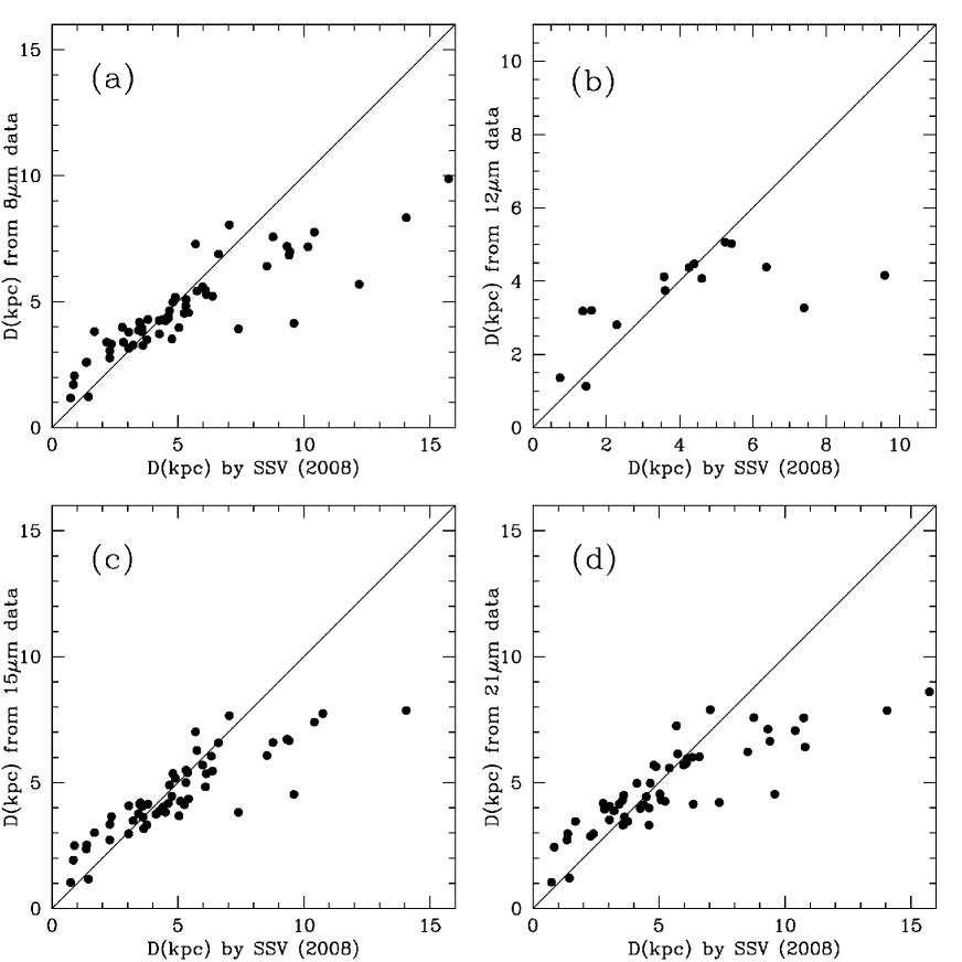
Figure 2: Distances of PNe determined by the present method plotted against the sample of calibrators compiled by SSV, for 4 the MSX bands: $8\,\mu$m (a), $12\,\mu$m (b), $15\,\mu$m (c), and $21\,\mu$m (d).

3 The calibration of a distance scale based on mid-infrared data

Statistical distances are generally based on the hypothesis that some nebular properties are constant or they can be evaluated from distance-independent data. The Shklovsky (1956) method for example, assumes that the ionized mass of the PN is invariant from object to object, and as a result, the distance can be expressed basically as a function of the incoming flux $F_{\lambda}$ and the nebular radius (Cahn & Kaler 1971, Milne & Aller 1975, Milne 1982, Daub 1982).

Apart from secondary effects involving physical parameters of the gas, such as electron temperature, the filling factor and the abundance of helium, the distance of a PN can be expressed by the following general equation:

$$D\propto F_{\lambda}^{\alpha}{\theta}^{\beta},$$ (3)

where $F_{\lambda}$ is the flux density $-$ or the brightness temperature $-$ $\theta$ is the nebular radius, and the constants $\alpha$ and $\beta$ depend on the wavelength considered. The empirical linear relationship between the radio and the infrared intensities discussed in Sect. 2 allows us to use the MSX flux densities to calibrate a new distance scale based on the parameters above. Equation (3) can be re-written in the following form:

$$\log D_{\rm MIR}=a_{\lambda}\log F_{\lambda}+b_{\lambda}\log{\theta}+c_{\lambda},$$ (4)

where $D_{\rm MIR}$ is the distance of the nebula, $F_{\lambda}$ is the MIR flux density, $\theta$ is the angular radius, and the constants a_λ, b_λ and c_λ depend on the wavelength.

Table 3: Distances of MSX counterparts of PNe listed in Ortiz et al. (2005) but not listed as a calibrator by Stanghellini et al. (2008, SSV), in alphabetical order.

#	PN	MSX	$\theta$	F8	F12	F15	F21	D8	D12	D15	D21	Dave
	name	name	(″)	(Jy)	(Jy)	(Jy)	(Jy)	(kpc)	(kpc)	(kpc)	(kpc)	(kpc)
1	H1-16	000.1899+04.3725	0.90	0.16	-	2.18	6.09	8.93	-	7.12	7.28	7.78
168	H1-17	358.3515+03.0903	0.45	0.47	1.52	3.15	10.28	9.75	7.79	8.16	8.05	8.44
165	H1-18	357.6250+02.6032	0.75	-	-	1.76	3.95	-	-	7.98	8.56	8.27
172	H1-19	358.9684+03.3993	0.70	0.15	1.45	0.95	4.99	10.04	7.05	9.51	8.28	8.72
171	H1-20	358.9850+03.2281	1.65	0.16	-	1.65	3.26	7.03	-	6.25	6.94	6.74
164	H1-23	357.6075+01.7961	1.25	0.86	-	1.95	3.51	5.88	-	6.57	7.47	6.64
151	H1-31	355.1810$-$02.9147	0.35	-	-	-	3.07	-	-	-	11.64	11.64
154	H1-35	355.7329$-$03.4718	0.55	1.55	3.46	7.14	31.77	7.32	5.91	6.23	5.76	6.31
148	H1-36	353.5114$-$04.9194	0.40	-	-	14.81	24.70	-	-	5.77	6.78	6.28
181	H1-40	359.7140$-$02.6919	0.65	1.08	1.81	4.74	16.86	7.30	6.76	6.53	6.35	6.73
10	H1-47	001.2950$-$03.0396	1.25	-	-	-	4.06	-	-	-	7.21	7.21
5	H2-11	000.7117+04.7025	0.75	0.16	-	-	4.34	9.65	-	-	8.37	9.01
21	H2-17	003.1935+03.4110	2.00	-	-	-	3.18	-	-	-	6.56	6.56
18	H2-20	002.7963+01.6947	1.70	0.13	-	-	3.03	7.20	-	-	7.00	7.10
41	Hb6	007.2758+01.8442	3.00	1.08	-	7.84	17.64	4.02	-	3.48	3.82	3.77
4	He2-250	000.7249+03.2473	2.50	0.12	-	1.12	-	6.31	-	6.00	-	6.16
73	K3-6	031.0357+04.1239	0.35	0.55	1.90	3.08	12.11	10.45	7.82	8.92	8.39	8.89
78	M1-12	235.3839$-$03.9208	0.90	0.90	2.50	3.02	7.99	6.64	5.70	6.57	6.82	6.43
173	M1-26	358.9597$-$00.7209	1.60	5.27	15.88	29.26	170.40	3.90	2.97	3.09	2.73	3.17
156	M1-30	355.9023$-$04.2676	1.75	0.16	-	1.16	4.27	6.92	-	6.69	6.39	6.66
17	M1-37	002.6807$-$03.4694	1.25	0.14	-	-	5.83	8.05	-	-	6.61	7.33
44	M1-40	008.3356$-$01.1042	2.15	1.25	2.21	8.86	16.92	4.47	4.72	3.77	4.30	4.31
51	M1-45	012.6066$-$02.7011	1.25	0.13	-	1.16	5.76	8.13	-	7.47	6.63	7.41
142	M2-4	349.8008+04.4649	1.00	0.19	-	1.99	4.15	8.37	-	7.04	7.71	7.70
25	M2-14	003.6194+03.1836	1.10	0.29	1.40	1.42	6.48	7.49	6.34	7.42	6.72	6.99
37	M2-31	006.0403$-$03.6209	2.00	0.19	-	1.73	3.86	6.39	-	5.80	6.26	6.15
58	M3-25	019.7518+03.2739	0.65	0.75	1.78	5.35	15.11	7.77	6.79	6.34	6.52	6.85
179	M3-44	359.3842$-$01.8140	2.00	-	-	1.17	12.36	-	-	6.39	4.75	5.57
56	M4-8	018.9038+03.6892	0.65	0.09	-	-	4.41	11.32	-	-	8.74	10.03
57	M4-10	019.2348$-$02.2459	0.60	0.11	-	1.40	3.43	11.22	-	9.08	9.52	9.94
46	NGC6537	010.0977+00.7396	2.35	3.64	4.50	18.12	40.34	3.58	3.80	3.06	3.40	3.46
68	Pe1-18	027.3446$-$02.1124	0.60	0.42	-	2.20	8.78	8.88	-	8.12	7.61	8.20
16	Th3-27	002.6923+04.2158	1.60	0.13	-	-	-	7.45	-	-	-	7.45

A comparison among the various statistical distances existing in the literature shows that some of them have significant biases when compared with each other. These effects can be minimized by calibrating the distance scale with objects in the Galactic bulge and/or in the Magellanic Clouds, which have distances determined more accurately. The method proposed by Cahn et al. (1992) was based on Shklovsky’s (1956) and improved by Daub (1982). In that study, 36 Galactic PNe with distances accurately determined by several methods was used to calibrate an empirical relationship between the distance and the nebular flux (of H$\beta$ or at 5 GHz, when available) and $\theta$. Eventually, that scale was re-calibrated using the Magellanic Clouds as a distance standard (Stanghellini et al. 2008, hereafter SSV) and as a result they obtained a method that describes the distance as a function of $T_{b}$ at 5 GHz and $\theta$. SSV also produced a list of distances of Galactic PNe to be used as calibrators in future distance scales.

The distance scale proposed in the present work was calibrated with the catalogue of Galactic PNe distances by SSV. Only PNe that appear both in Table 1 of SSV as well as in the compilation of MSX counterparts of PNe (Table 3 of Ortiz et al. 2005) have been considered (67 objects, Table 2). PNe with bad-quality MSX photometry and/or without size measurements have been discarded. In order to obtain the coefficients of equation 4, we fitted the SSV distances, MSX flux densities and the nebular radii using the least-squared method. The nebular radii $\theta$ used in this work have been preferentially extracted from Siódmiak & Tylenda (2001), obtained with the VLA. In the cases where this measurement was not available, $\theta$ was taken from the compilation of SSV. Among the 67 PNe used in the calibration, there are only 26 objects with apparent radii listed both in Siodmiak & Tylenda as well as in SSV and, among these, there are only 4 discrepant determinations of $\theta$: M2-16, M3-14, Hb5, and NGC2440. Apart from these few exceptions the agreement between the two radii (optical and radio) is excellent.

Table 1 presents the MSX bands, their isophotal wavelength (Egan et al. 1999) and the fitting coefficients obtained with the least-squared method, where the distance $D$ must be given in kiloparsecs, $F_{\lambda}$ in Jansky, and $\theta$ in arc seconds. Because the flux quality varies from object to object and from band to band, the number $N$ of PNe used in each fit is not the same. A simple examination of Table 1 reveals that the coefficients $a_{\lambda}$, $b_{\lambda}$ and $c_{\lambda}$ show a non-negligible variation with the wavelength. The values relative to 12 $\mu$m are the most uncertain because of the small number of objects with good-quality photometry, caused by the lack of sensitivity in this band. If one takes the average value of these coefficients, equation 3 would be written with $\langle\alpha\rangle=-0.23$ and $\langle\beta\rangle=-0.32$.

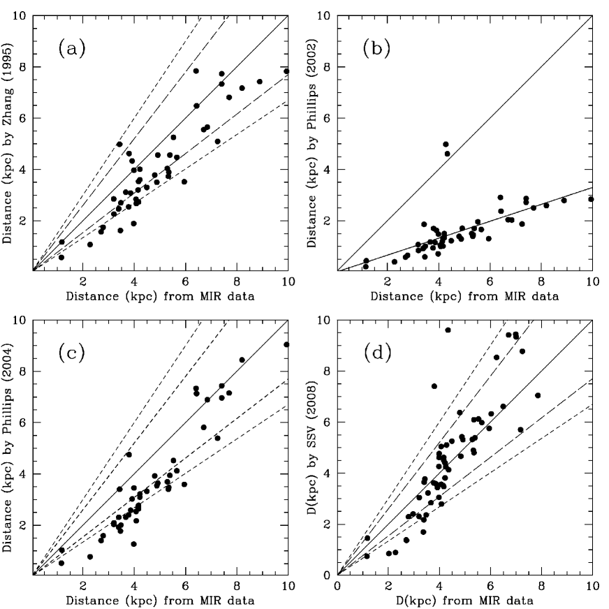
Figure 3: Distances of PNe determined by the present method plotted against other distance scales by: (a) Zhang (1995), (b) Phillips (2002), (c) Phillips (2004), and (d) Stanghellini et al. (2008, SSV). The auxiliary dashed lines drawn on both sides of the identity line represent a deviation of 30% and 50% from equality.

4 Results

In Table 2, we list the original data used in the fitting of equation 4 and the various distances, obtained by SSV and in this work. The columns are: (1) Ordering number, according to Ortiz et al. (2005); (2) Name; (3) MSX name; (4) Angular radius (″); (5$-$8) MSX flux densities (Jansky); (9-12) Distance (in kpc) obtained from the MSX bands centred at 8, 12, 15 and 21 $\mu$m, respectively; (13) Average Distance (kpc); (14) Distance according to SSV. A comparison between $D_{\mathrm{SSV}}$ and $D_{\mathrm{ave}}$ is shown in Fig. 3d. The points are approximately dispersed near the identity line within $\pm$50%. The scattering of the points results mainly from two sources of errors: (i) intrinsic errors of the present method (including errors in the data); (ii) errors in $D_{\rm SSV}$, estimated as $\sim$30% in the original reference. According to the authors, this figure is similar to that observed in other distance scales and cannot be significantly reduced by using better calibrators.

Among the factors that contribute to the scattering seen in Fig. 3 is the error associated with the nebular radius $\theta$. Fortunately, the majority of the $\theta$ measurements used in our fit were determined with the VLA, which gives spatial resolution superior to any optical measurement obtained by ground-based telescopes. The error in the determination of $D_{\mathrm{MIR}}$ caused by an error in $\theta$ is:

$$\left(\frac{{\sigma}_{D}}{D}\right)_{\mathrm{MIR}}=|b_{\lambda}|\frac{{\sigma}_{\theta}}{\theta},$$ (5)

where ${\sigma}_{\theta}$ is the error bar associated with the measurement of the nebular radius. Assuming ${\sigma}_{\theta}=1$ ″– corresponding to a typical seeing at the visual wavelengths – the error in $D_{\mathrm{MIR}}$ calculated with equation 5 and $b_{\lambda}$ taken from Table 1 is 30% – 40% for a PN with $\theta=1$″. This error drops down to a half of this value for a PN with $\theta=2$″and so on.

The errors in the MSX flux densities are small, between 3% and 6% for the bands listed in Table 1 (Egan et al. 1999). Thus, this source of error does not play an important role in the evaluation of the total error in $D$, especially when compared to the contribution of the error in $\theta$.

Table 4: Distances of PNe observed by GLIMPSE. The original data were extracted from Kwok et al. (2008, first set of data) and Zhang & Kwok (2009, second set below). The columns are (1) PNG name; (2) other name, (3) MSX name; (4) integrated flux density (Jansky) at 8 $\mu$m, corrected (see text); (5) nebular radius, in arc seconds; (6) $D_{\rm MIR}$ (kpc).

PNG name	Other name	MSX name	F8(Jy)	$\theta$(″)	$D_{\rm MIR}$(kpc)
PNG010.1+00.7	NGC6537	MSX010.0997+00.7396	4.968	6.0	2.35
PNG011.7$-$00.6	NGC6567	MSX011.7438$-$00.6502	2.225	6.0	2.71
PNG018.6$-$00.0	G018.6$-$00.0		40.508	60.0	0.67
PNG035.5$-$00.4	G035.5$-$00.4	MSX035.5653$-$00.4913	0.155	5.0	4.61
PNG040.3$-$00.4	G040.3$-$00.4		0.198	10.0	3.37
PNG055.5$-$00.5	M1$-$71	MSX055.5067$-$00.5579	1.290	5.0	3.19
PNG056.4$-$00.9	K3$-$42		0.052	3.5	6.42
PNG062.4$-$00.2	M2$-$48		0.028	3.5	7.16
PNG295.7$-$00.2	G295.7$-$00.2		8.294	30.0	1.15
PNG296.8$-$00.9	G296.8$-$00.9		0.029	5.0	6.19
PNG298.4+00.6	G298.4+00.6		23.292	90.0	0.63
PNG300.2+00.6	He2$-$83	MSX300.2787+00.6627	0.331	5.0	4.04
PNG300.4$-$00.9	He2$-$84		0.025	5.0	6.32
PNG315.0$-$00.3	He2$-$111	MSX315.0301$-$00.3701	0.267	7.5	3.58
PNG318.9+00.6	G318.9+00.6	MSX318.9321+00.6956	0.166	10.0	3.48
PNG333.9+00.6	G333.9+00.6	MSX333.9294+00.6858	1.057	22.5	1.84
PNG343.9+00.8	H1$-$5	MSX343.9919+00.8347	0.869	6.0	3.19
PNG000.0$-$01.3	G000.0$-$01.3		0.022	5.8	6.11
PNG000.1$-$01.7	G000.1$-$01.7		0.011	6.0	6.80
PNG000.3$-$01.6	G000.3$-$01.6		0.011	4.0	7.97
PNG000.5+01.9	K6$-$7		0.029	5.0	6.19
PNG000.9$-$01.0	G000.9$-$01.0		0.025	4.5	6.59
PNG000.9$-$01.8	G000.9+01.8		0.013	2.5	9.27
PNG001.0$-$01.9	K6$-$35		0.019	6.5	6.01
PNG001.6$-$01.1	G001.6$-$01.1		0.033	4.8	6.13
PNG002.0+00.7	G002.0+00.7		0.043	4.0	6.29
PNG002.1$-$00.9	K5$-$35	MSX002.1198$-$00.9610	0.238	6.0	3.99
PNG002.1$-$01.1	G002.1$-$01.1		0.016	3.0	8.31
PNG002.2$-$01.2	G002.2$-$01.2		0.024	5.5	6.14
PNG003.4+01.4	G003.4+01.4		0.021	5.0	6.53
PNG003.5$-$01.2	G003.5$-$01.2	MSX003.5794$-$01.2219	1.188	5.5	3.12
PNG003.5+01.3	G003.5+01.3	MSX003.5562+01.3532	0.057	5.0	5.49
PNG003.6$-$01.3	G003.6$-$01.3		0.025	5.0	6.32
PNG004.3$-$01.4	G004.3$-$01.4		0.032	4.0	6.62
PNG004.8$-$01.1	G004.8$-$01.1	MSX004.8343$-$01.1940	0.133	5.8	4.47
PNG006.1+00.8	G006.1+00.8		0.030	5.5	5.92
PNG353.9+00.0	G353.9+00.0		0.065	5.0	5.37
PNG355.6+01.4	G355.6+01.4	MSX355.6143+01.4111	0.095	5.0	5.03
PNG356.0$-$01.4	G356.0$-$01.4		0.032	5.5	5.85
PNG356.9+00.9	G356.9+00.9	MSX356.9505+00.9112	0.228	5.0	4.32
PNG357.5+01.3	G357.5+01.3		0.105	5.0	4.94
PNG357.7+01.4	G357.7+01.4		0.012	3.0	8.77
PNG358.2$-$01.1	Al2$-$L		0.062	9.5	4.22
PNG358.8$-$00.0	Terz2022		55.728	40.0	0.74
PNG359.1$-$01.7	He1$-$191	MSX359.1155$-$01.7195	0.303	7.5	3.51

Table 3 contains the distances calculated for PNe present in the sample of Ortiz et al. (2005), but absent in the list of SSV. The columns are: (1) Ordering number, according to Ortiz et al. (2005); (2) Name; (3) MSX name; (4) Angular radius (″); (5$-$8) MSX flux densities (Jansky); (9-12) Distance (in kpc) obtained from the flux density at 8, 12, 15 and 21 $\mu$m, respectively; (13) Average Distance (kpc). In order to compare our results with others, we merged Tables 2 and 3 and plotted the average distance obtained by the present method against other values given by methods based on radio fluxes, extracted from several references. The distance scale proposed by Zhang (1995) was based on a correlation between $T_{b}$ and the nebular radius (an upgrade to the Shklovsky method), and calibrated with a sample of 134 “standard” nebulae. Figure 3 shows that Zhang’s distance scale is about $\sim 20$% shorter than ours (and SSV, by extension). Phillips (2002) proposed a statistical method similar to Zhang’s (1995), but calibrated it with a sample of nearby ($D<0.7$ kpc) PNe. His distance scale was based on a revised relationship between the surface brightness and the nebular radius and, when compared to our results (Fig. 3, top-right), his method produces distances shorter by a factor $\sim 3$. A revision of that method was eventually proposed by Phillips (2004), that assumes a relationship between the nebular luminosity at 5 GHz and the nebular brightness temperature, $T_{b}$. A comparison between our results and the distances produced by the latter method ($D_{\rm Ph04}$) is presented in the bottom-left panel of Fig. 3: there seems to be a bias associated with $D_{\rm MIR}<6$ kpc, but both methods agree within $\sim 30$% beyond 6 kpc.

4.1 Distances obtained from other mid-infrared surveys: Spitzer

The present method was calibrated with nebular flux densities of the MSX survey centred at 8.3, 12.1, 14.7 and 21.3 $\mu$m. This calibration (equation 4 and Table 1) can be extended to other surveys if their effective wavelength is similar to MSX. As an example, we present in this section distances of PNe detected by the Spitzer satellite during the GLIMPSE Legacy Survey (Fazio et al. 2004). As mentioned in the introduction, the IRAC camera had one band centred at $\lambda=8.0\,\mu$m, not very different from the MSX band ’A’ centred at $\lambda=8.3\,\mu$m. Differently from “point-source surveys”, GLIMPSE recorded full images of PNe and the flux density integrated over the total nebular solid angle can be easily computed and used to produce distances by our method.

Kwok et al. (2008) and Zhang & Kwok (2009) obtained integrated flux densities of over 60 PNe with sensitivity superior to MSX. A comparison between the GLIMPSE and MSX fluxes of a sample of 22 PNe showed the existence of a bias expressed as: $F({\rm IRAC\,8.0})/F({\rm MSX\,8.3})=0.90\pm 0.36$ (Zhang & Kwok 2009). We applied this correction factor to GLIMPSE flux densities at 8.0 $\mu m$ to calculate $D_{\rm MIR}$ and listed these results in Table 4. The first set of data, from row 1 to 17, refers to PNe situated along the Galactic disc, between $10^{\circ}-60^{\circ}$ away from the Galactic centre. The second set, from the 18th row on, refers to PNe situated within $5^{\circ}$ from the Galactic centre, i.e. seen against the bulge. A simple inspection of these two sets of objects shows that, on average “disc” PNe have smaller distances when compared to “bulge” objects. Actually the distances of the “disc” PNe show a wide range of values, from 0.6 to 7.2 kpc. On the other hand, the distances of the “bulge” PNe are more homogeneous, from 3.1 to 9.3 kpc. The only exception is the object named PNG358.8-00.0 (Terz2022): considering its large infrared flux and apparent size, it is a clear example of a nearby object seen against the bulge. Table 4 also shows how deep is the Spitzer survey when compared to MSX: the faintest flux density at 8 $\mu$m in Tables 2 and 3 is $F_{8}=0.11$ Jansky (object M4-10), whereas Table 4 contains plenty of nebulae with one-tenth of this value.

5 Conclusions

In this work we proposed a distance scale of planetary nebulae based on mid-infrared flux densities and the nebular apparent size. A study of two distance-independent nebular parameters – the brightness temperature at 5 GHz and the mid-infrared specific intensity $I_{\lambda}$ – showed that these two characteristics are very well correlated. This relationship, as well as the similar formulation of the distance scale – $D$ as a function of the nebular monochromatic specific intensity and its size – allows us to state that the reliability of our method is similar to SSV’s. In fact, a comparison between the nebular distances calculated by both methods showed that they produce similar results within 50%. Nevertheless, since both methods are statistical, each of them might be accurate only within the natural limitation imposed by the set of hypotheses assumed to be valid for the whole set of PNe, but that may vary significantly from object to object. These variations include the different effect of the various spectral features (continuum, atomic lines, molecular bands) on the final flux, deviations from sphericity, etc. However, like in many statistical methods, particular deviations from the average may not introduce significant errors in the distance scale, but only in the error bars. As an example, according to SSV, excluding bipolar PNe from the sample would not change their distance scale by more than 5%, and a similar figure is expected here. On the other hand, variations of this kind may affect the distance error bars, and a comparison between the distances determined by SSV and our results showed that are equal within $\pm$50%.

Although the effects of the [C/O] ratio – either of the gas or on the grain surface – on the nebular spectrum are well known, we could not detect its effect on the distance scale proposed, because of the small number of objects in our sample with observed C and/or O molecular features.

As an example of application of the present method, we derived distances of a sample of PNe observed by the Spitzer infrared telescope. This distance scale can be extended to any other database containing nebular radii and flux densities near 8, 12, 15, and 21 $\mu$m, such as IRAS, ISOGAL, and future infrared surveys of this kind.

References

- [1] Barlow, M.J., 1987, MNRAS, 227, 161
- [2] Blöcker, T. & Schönberner, D., 1990, A&A, 240, L11
- [3] Blommaert, J.A.D.L., van der Veen, W.E.C.J. & Habing, H.J., 1993, A&A, 267, 39
- [4] Cahn, J.H. & Kaler, J.B., 1971, ApJS, 22, 319
- [5] Cahn, J.H., Kaler, J.B., Stanghellini, L., 1992, A&AS, 94, 399
- [6] Casassus, S., Roche, P.F., Aitken, D.K. & Smith, C.H., 2001a, MNRAS, 327, 744
- [7] Casassus, S., Roche, P.F., Aitken, D.K. & Smith, C.H., 2001b, MNRAS, 320, 424
- [8] Daub, C.T., 1982, ApJ, 260, 612
- [9] Egan, M.P., Price, S.D., Shipman, R.F. & Tedesco, E., 1997, A&AS, 29, 1294
- [10] Egan, M.P., Price, S.D., Moshir, M.M. et al., 1999, The Midcourse Space Experiment Point Source Catalog Version 1.2 Explanatory Guide, AFGL Tech. Rep. AFRL-VS-TR-1999-1522
- [11] Fazio, G.G., Hora, J.L., Allen, L.E., Ashby, M.L.N., Barmby, P., Deutsch, L.K., Huang, J.-S., Kleiner, S., Marengo, M., Megeath, S.T. et al., 2004, ApJS, 154, 10
- [12] Gillett, F.C., Low, F.J. & Stein, W.A., 1967, ApJ, 149, L97
- [13] Guglielmo, F., Le Bertre, T. & Epchtein, N., 1998, A&A, 334, 609
- [14] Harris, H.C., Dahn, C.C., Monet, D.G. & Pier, J.R., 1997, in IAU Symp. 180: Planetary Nebulae, eds. H.J. Habing & H. Lamers (Kluwer: Dordrecht), p. 40
- [15] Kwok, S., 1985, ApJ, 290, 568
- [16] Kwok, S., 1989, in IAU Symp. 131, Planetary Nebulae, ed. S. Torres-Peimbert (Kluwer: Reidel), 401
- [17] Kwok, S., Zhang, Y., Koning, N., Huang, H.-H. & Churchwell, E., 2008, ApJS, 174, 426
- [18] Maciel, W.J. & Pottasch, S.R., 1980, A&A, 88, 1
- [19] Marten, H. & Schoenberner, D., 1991, A&A, 248, 590
- [20] Méndez, R.H., Kudritzki, R.P., Herrero, A., Husfeld, D. & Groth, H.G., 1988, A&A, 190, 113
- [21] Milne, D.K., 1982, MNRAS, 200, 51P
- [22] Milne, D.K. & Aller, L.H., 1975, A&A, 38, 183
- [23] Omont, A., Gilmore, G.F., Alard, C., Aracil, B., August, T., Baliyan, K., Beaulieu, S., Bégon, S., Bertou, X., Blommaert, J.A.D.L. et al., 2003, A&A, 403, 975
- [24] Ortiz, R., Lorenz-Martins, S., Maciel, W.J., Rangel, E.M., 2005, A&A, 431, 565
- [25] Phillips, J.P., 2002, ApJS, 139, 199
- [26] Phillips, J.P., 2004, MNRAS, 353, 589
- [27] Schönberner, D., 1981, A&A, 103, 119
- [28] Schönberner, D., 1983, ApJ, 272, 708
- [29] Shklovsky, I., 1956, Astr. Zh., 33, 222
- [30] Siódmiak, N. & Tylenda, R., 2001, A&A, 373, 1032
- [31] Stanghellini, L., Shaw, R.A. & Villaver, E., 2008, ApJ, 689, 194 (SSV)
- [32] Stasińska, G. & Szczerba, R., 1999, A&A, 352, 297
- [33] Terzian, Y., 1997, in IAU Symp. 180: Planetary Nebulae, eds. H.J. Habing & H. Lamers (Kluwer: Dordrecht), p.29
- [34] Volk, K., 1992, ApJS 80, 347
- [35] Zijlstra, A.A., Pottasch, S.R. & Bignell, C., 1989, A&AS, 79, 329
- [36] Zhang, C.Y., 1995, ApJS, 98, 659
- [37] Zhang, C.Y. & Kwok, S., 1990, A&A, 237, 479
- [38] Zhang, C.Y. & Kwok, S., 1993, ApJS, 88, 137
- [39] Zhang, C.Y. & Kwok, S., 1991, A&A, 250, 179
- [40] Zhang, C.Y. & Kwok, S., 2009, ApJ, 706, 252