Mixed Multiscale Finite Volume Methods for Elliptic Problems in Two-phase Flow Simulations

ABSTRACT

We develop a framework for constructing mixed multiscale finite volume methods for elliptic equations with multiple scales arising from flows in porous media. Some of the methods developed using the framework are already known [20]; others are new. New insight is gained for the known methods and extra flexibility is provided by the new methods. We give as an example a mixed MsFV on uniform mesh in 2-D. This method uses novel multiscale velocity basis functions that are suited for using global information, which is often needed to improve the accuracy of the multiscale simulations in the case of continuum scales with strong non-local features. The method efficiently captures the small effects on a coarse grid. We analyze the new mixed MsFV and apply it to solve two-phase flow equations in heterogeneous porous media. Numerical examples demonstrate the accuracy and efficiency of the proposed method for modeling the flows in porous media with non-separable and separable scales.

1 Introduction

Subsurface flows are often affected by heterogeneities in a wide range of length scales. This causes significant challenges for subsurface flow modeling. Geological characterizations that capture these effects are typically developed at scales that are too fine for direct flow simulations. Usually, upscaled or multiscale models are employed for such systems. In upscaling methods, the original model is coarsened by numerically homogenizing parameters (e.g., permeability). The simulation is performed using the coarsened model, which may differ from the underlying fine-scale model. In multiscale methods, the fine-scale information is carried throughout the simulation and the coarse-scale equations are generally not expressed analytically, but rather formed and solved numerically.

Various numerical multiscale approaches for flows in porous media have been developed during the past decade. A multiscale finite element method (MsFEM) was introduced in [18] and takes its origin from the pioneering work [5]. Its main idea is to incorporate the small-scale information into finite element basis functions and capture their effect on the large scales via finite element computations. The MsFEM in [18] shares some similarities with a number of multiscale numerical methods, such as residual free bubbles [6], variational multiscale method [19], two-scale conservative subgrid approaches [3], heterogeneous multiscale method [15] and multiscale discontinuous Galerkin method [31]. Chen and Hou have applied the MsFEM idea in combination with a mixed finite element formulation to propose a mixed MsFEM [8]. Recently, Arbogast et al. [4] used domain decomposition approach and variational mixed formulation to develop a multiscale mortar mixed MsFEM. Jenny et al. [20] have used the ideas in [18] and finite volume framework to design a multiscale finite volume method (MsFV). The MsFV and its variants have proved successful in reservoir simulations.

Here we develop a framework for constructing mixed MsFV methods, which uses ideas from the mixed finite volume methods [24, 25, 26], multi-point flux approximations (MPFA) [2, 16], and mixed MsFEM. The mixed MsFV are mass conservative methods, which is an important property of the discretizations used in subsurface flow simulations (see [11] for related discussion). The important feature of the mixed finite volume methods is the direct approximation of the velocity, that is, specially constructed discrete spaces are used to approximate the velocity unknowns. We propose a novel way to construct multiscale velocity basis functions that are well suited for parallel computation. Mixed MsFEM reduces the system of coupled equations for pressure and velocity to a system only for the pressure. However, the reduction process is computational expensive and has some restrictions when the global mass matrix in mixed MsFEM is large. In the mixed MsFV, we compute the inverse of each local mass matrix instead of global mass matrix and get effective coarse-scale transmissibilities. This computation is cheap and efficient. In the MsFV proposed in [20], two sets of multiscale basis functions are computed: the first set of basis functions is to approximate pressure and the second set of basis functions is required to construct a conservative fine-scale velocity field. Only one set of multiscale basis functions is constructed in the mixed MsFV and the span of the basis functions are to approximate the velocity. Piecewise constant is used for pressure basis in the mixed MsFV. Hence the computation for basis functions in the mixed MsFV is less expensive than the MsFV. To the best of our knowledge, the mixed MsFV is a new numerical multiscale method.

Boundary effect is a great issue in many multiscale methods (e.g., [18, 8]). When we construct the multiscale basis functions in the mixed MsFV, we can use constant boundary condition for basis equations and obtain local multiscale basis. We find that the local multiscale basis in the mixed MsFV has the similar merit to the multiscale basis using oversampling technique developed in [18] and they are able to reduce the boundary effect greatly. The mixed MsFV using local multiscale basis works well for most multiscale problems and particularly for the case of separable scales (e.g., periodic media). Furthermore, we can employ global information for the multiscale basis functions of the mixed MsFV. The global information usually represents long range features of flows and is used to construct multiscale basis functions. The global information is needed in the case of strong non-separable scales and renders much better accuracy than local multiscale approaches [1].

The proposed mixed MsFV in some extend inherits the advantages of the mixed MsFEM and MsFV and alleviates the drawbacks of them without increase of the computational cost. Moreover, this method and its generalizations are well suited for computation on unstructured grids and can be easily incorporated in production reservoir simulators. For example, to construct the velocity basis no geometric information is necessary. The pressure basis can be computed using only the local matrices if it consists of discrete harmonic functions as demonstrated in [14]. Detailed description is provided in [27].

The rest of the paper is organized as follows. Section 2 is devoted to formulating a standard mixed finite volume method for a model elliptic equation. In Section 3, we apply the methodology of the mixed finite volume method to develop a mixed MsFV method. Here we design a new multiscale velocity basis function, analyze the proposed mixed MsFV, and address some computational issues. In Section 4, we generalize the approach applied in Section 3 to derive our first mixed MsFV method and show how given a mixed FV method we can derived a corresponding mixed MsFV. Several examples are given to demonstrate how the framework can be used to develop new mixed MsFV methods. In Section 5, we apply a mixed MsFV to incompressible two-phase flows in porous media with continuum scales and separable scales. Finally, some comments and conclusions are made.

2 Mixed finite volume method formulation for a model problem

We first define notations for function spaces used in the paper.

$$L^{2}(\Omega) = \{f(x)|\int_{\Omega}|f(x)|^{2}dx<\infty\},$$

$$H^{1}(\Omega) = \{f(x)|f(x)\in L^{2}(\Omega)\quad\text{and}\quad\nabla f(x)\in[L^{2}(\Omega)]^{d}\},$$

$$H(div,\Omega) = \{f(x)|f(x)\in[L^{2}(\Omega)]^{d}\quad\text{and}\quad\text{div}(f(x))\in L^{2}(\Omega)\}.$$

We consider the following model elliptic equation,

$$\begin{cases}\begin{split}-\text{div}(k(x)\nabla p)&=f(x)\ \ \text{in}\ \ \Omega,\\ k(x)\nabla p\cdot n&=0\ \ \text{on}\ \ \partial\Omega,\\ \int_{\Omega}pdx&=0,\end{split}\end{cases}$$ (2.1)

where $\Omega$ is a domain in $\mathbb{R}^{d}$, $d=2$ or $3$ and $f\in L^{2}(\Omega)$. Equation (2.1) is used to model many physical processes, for example, fluid flow in porous media. The coefficient $k(x)$ represents the permeability and is often heterogeneous. Here $p$ represents pressure.

We define velocity $u(x)=-k(x)\nabla p$. To simplify presentation, we shall not write the spatial variables $x$ for functions when no ambiguity occurs. Then (2.1) can be rewritten as a first order system

$$\begin{cases}\begin{split}k^{-1}u+\nabla p&=0\\ \text{div}(u)&=f.\end{split}\end{cases}$$ (2.2)

The weak mixed formulation for (2.2) is:
Find $\{u,p\}\in\mathcal{U}\times\mathcal{P}$ such that

$$\begin{cases}\begin{split}\int_{\Omega}k^{-1}u\cdot vdx+\int_{\Omega}\nabla p\cdot vdx&=0,\quad&\forall v\in\mathcal{V},\\ \int_{\Omega}\text{div}(u)qdx&=\int_{\Omega}fqdx\quad&\forall q\in\mathcal{Q},\end{split}\end{cases}$$ (2.3)

where $\mathcal{U}=H(div,\Omega)$, $\mathcal{P}=H^{1}(\Omega)$, $\mathcal{V}=(L^{2}(\Omega))^{d}$, and $\mathcal{Q}=L^{2}(\Omega)$.

There are different ways to construct a discretization of equation (2.3). One can try to find the approximations such that $\{u_{h},p_{h}\}\in H(div,\Omega)\times H^{1}(\Omega)$ [30]. Unfortunately these discretizations are computationally expensive and are only applicable on very restrictive grids. Frequently dual mixed finite element methods are used [7, 29] to construct the discretization $\{u_{h},p_{h}\}\in H(div,\Omega)\times L^{2}(\Omega)$. We will consider a class of methods that are related to the primal mixed finite element methods [29], i.e., the discretizations we seek are $\{u_{h},p_{h}\}\in\mathcal{U}_{h}\times\mathcal{P}_{h},\,\,\mathcal{U}_{h}\subset\left(L^{2}(\Omega)\right)^{d},\,\mathcal{P}_{h}\subset H^{1}(\Omega)$ with additional conservation enforced on particular volumes. These methods are close related to the standard cell-centered finite volume method and several multi-point flux approximation (MPFA) methods that generalize it. We will refer such approximations as mixed finite volume methods.

We assume that two grids are defined: primary grid $\mathcal{T}_{h}$ and dual grid $\mathcal{D}_{h}$. Usually the primary grid is used to approximate the scaler variable $p$, and the dual mesh is used to construct the discretization of the velocity. Different examples of primary and dual grids can be found in [2, 16, 24, 25, 26]. Consider the discrete problem:
Find $\{u_{h},p_{h}\}\in\mathcal{U}_{h}\times\mathcal{P}_{h}$ such that

$$\begin{cases}\begin{split}\int_{\Omega}k^{-1}u_{h}\cdot v_{h}dx+\int_{\Omega}\nabla_{h}p_{h}\cdot v_{h}dx&=0,\quad\forall v_{h}\in\mathcal{V}_{h},\\ \int_{\Omega}\text{div}_{h}(u_{h})qdx&=\int_{\Omega}fq_{h}dx.\quad\forall q_{h}\in\mathcal{Q}_{h},\end{split}\end{cases}$$ (2.4)

A particular mixed finite volume method will be fully described if we define the grids, the approximation spaces, and the operators $\nabla_{h}$, and $\text{div}_{h}$. The operator $\text{div}_{h}$ can be defined in the following way:

$$\int_{\Omega}\text{div}_{h}(u_{h})q_{h}\,dx:=\sum_{V\in\mathcal{T}_{h}}\sum_{E\in\partial V}\int_{E}u_{h}\cdot n_{E}q_{h}\,ds$$ (2.5)

with $\mathcal{Q}_{h}$ the space of piece-wise constants on the volumes $V$ from the primary grid and $E$ is an edge in 2-D or face in 3-D in $\partial V$. Here $n_{E}$ denotes the outward normal vector to $E$.

In the paper, we focus on 2-D case. The 3-D case is a straightforward extension of 2-D case.

We give an example of mixed finite volume methods as following.

Example 1 (Mixed FV 1).

We assume that the primary grid $\mathcal{T}_{h}$ consists of rectangles, and the dual grid $\mathcal{D}_{h}$ is also rectangular, but with vertexes the cell centers. The discrete space for the scalar variable, $\mathcal{P}_{h}=\mathcal{Q}_{h}$, consists of piecewise constants and is defined on the primary grid, The approximation space for the vector variable, $\mathcal{U}_{h}=\mathcal{V}_{h}$, is the space of piece-wise constants vector constants with continuous normal components and is defined on the dual mesh. Consider one dual cell $D=D_{i}\cup D_{j}\cup D_{k}\cup D_{l}$ (see Figure 2.1). The four functions, $e_{ij}$, $e_{ik}$, $e_{jl}$ and $e_{kl}$ are defined with the relations

$$\int_{l_{rt}}e_{pq}\cdot n_{rt}\,dx=\delta_{pq,rt},$$

where $pq$ and $rt$ can be any element of the set $I_{D}=\{ij,\,ik,\,jl,\,jk\}$. It is easy to see that $\{e_{pq}\},\,pq\in I_{D}$ are linearly independent and therefore form a basis of $\mathcal{U}_{h|D}$. The degrees of freedom are the integrals of the flux, i.e, the numbers $v_{pq}=\int_{l_{pq}}v\cdot n_{pq}\,dx\quad pq\in I_{D}$. Then for any $v\in\mathcal{U}_{h}$, $v_{|D}=\sum_{pq\in I_{D}}v_{pq}e_{pq}$. The operator $\nabla_{h}$ is given by:

$$\int_{\Omega}\nabla_{h}p_{h}\cdot v_{h}\,dx=\sum_{V\in\mathcal{T}_{h}}\sum_{E\in\partial V}\int_{E}v_{h}\cdot n_{E}\,[p_{h}]_{E}\,dx,$$ (2.6)

where

$$[p]_{E}=\lim_{t\rightarrow 0\atop t>0}(p(x+t{\bf n}_{E})-p(x-t{\bf n}_{E}))$$

and the direction of $n_{E}$ is from left to right or from bottom to top in 2-D. Note that from the first equation of (2.4) we can express

$$M\vec{u}=\vec{p},$$ (2.7)

with $\vec{u}^{T}=[u_{ij},u_{ik},u_{jl},u_{kl}]^{T}$, $\vec{p}=[p_{i}-p_{j},p_{i}-p_{k},p_{j}-p_{l},p_{k}-p_{l}]^{T}$, and $M$ a $4\times 4$ matrix. We solve for $\vec{u}$ and plug the result in the second equation of (2.4) to get the final discretization.

For Example 1, We can rewrite equation (2.5) as

$$\sum_{V\in\mathcal{T}_{h}}\sum_{E\in V}\int_{E}u_{h}\cdot n_{E}[q_{h}]_{E}=-\int_{\Omega}fq_{h}dx.$$

which shows that the matrix of the discretization is symmetric. We note that $\mathcal{P}_{h}$ in Example 1 is not subspace of $H^{1}(\Omega)$. Our approximation of $\nabla p$ is nonconforming.

Figure 2.1: A dual cell $D$

The Example 1 is a straightforward generalization of the standard cell-centered finite volume method on structured rectangular meshes [25]. In fact, if the coefficient $k(x)$ in (2.1) is a scalar function, then this method coincides with the standard cell-centered finite volume method.

We need the matrix $M$ in equation (2.7) to have the appropriate dimensions and to be invertible in order to have a well defined discretization in Example 1. We state these condition for future reference:

1. $dim(\mathcal{P}_{h})+dim(\mathcal{U}_{h})=dim(\mathcal{Q}_{h})+dim(\mathcal{V}_{h})$;

2. Matrix $M$ is invertible.

We will follow Example 1 to derive a new mixed MsFV method in the next section.

3 A new mixed multiscale finite volume method

In order to describe the multiscale finite element method, we assume that the grids $\mathcal{T}_{H}$ and $\mathcal{D}_{H}$ are coarse grids and that there exist an underlying fine grid containing the fine-scale information. Figure 3.2 depicts the rectangle primary coarse grid and dual coarse grid. The velocity $u$ is discretized on the interfaces $\mathcal{E}_{H}$ of primary grid, e.g., $E_{ij}$ in Figure 3.2, and the pressure $p$ is discretized on cell-centers of the primary mesh / the vertices of the dual grid, e.g, vertex $i,j,k,l$ in Figure 3.2.

Define the discrete space for pressure to be $\mathcal{P}_{H}=\mathcal{Q}_{H}$, the space of piecewise constants on $\mathcal{T}_{H}$, and for velocity to be $\mathcal{U}_{H}=\mathcal{V}_{H}$, a multiscale finite element space with continuous normal on $\mathcal{E}_{H}$ that will be defined in Subsection 3.1. Then the mixed multiscale finite volume formulation for Equation (2.3) reads:
Find $\{u_{H},p_{H}\}\in\mathcal{U}_{H}\times\mathcal{P}_{H}$ such that

$$\begin{cases}\begin{split}\int_{\Omega}k^{-1}u_{H}\cdot v_{H}dx+\sum_{E\in\mathcal{E}_{H}}\int_{E}v_{H}\cdot n_{E}[p_{H}]_{E}dx&=0\ \ \forall v_{H}\in\mathcal{U}_{H},\\ \sum_{V\in\mathcal{T}_{H}}\int_{\partial K_{i}}u_{H}\cdot nq_{H}dx&=\int_{\Omega}fq_{H}dx\ \ \forall q_{H}\in\mathcal{P}_{H},\end{split}\end{cases}$$ (3.8)

where $[p_{H}]_{E}$ is the jump of $p_{H}$ across the interface $E$ and defined in Example 1. It is clear from equation (3.8) that the operators $\text{div}_{H}$ and $\nabla_{H}$ are defines as follows:

$$\int_{\Omega}\nabla_{H}p_{H}\cdot v_{H}\,dx=\sum_{E\in\mathcal{E}_{H}}\int_{E}v_{H}\cdot n_{E}\,[p_{H}]_{E}\,dx,$$ (3.9)

and

$$\int_{\Omega}\text{div}_{h}(u_{h})q_{h}\,dx=\sum_{V\in\mathcal{T}_{h}}\sum_{E\in\partial V}\int_{E}u_{h}\cdot n_{E}q_{h}\,ds$$ (3.10)

Clearly $u_{H}\in L^{2}(\Omega)$ and $p_{H}\in L^{2}(\Omega)$. By a similar argument as in Example 1, the discrete system of (3.8) is symmetric.

3.1 A new multiscale velocity basis function

In order to complete the derivation of the method from (3.8), we need to define velocity basis functions. In this subsection we design multiscale velocity basis functions associated with interfaces of $\mathcal{E}_{H}$.

Let $E_{ij}\in\mathcal{E}_{H}$ be any interface and $\Omega_{ij}$ (green part in Figure 3.2) be an open set bounded by edges $e_{ij}^{l}$, $e_{ij}^{r}$, $e_{ij}^{b}$ and $e_{ij}^{t}$. We construct a multiscale basis function $\phi_{ij}$ associated to the interface $E_{ij}$ as following:

$$\begin{cases}\begin{split}-\text{div}(k\nabla\phi_{ij})&=0\ \ \text{in}\ \ \Omega_{ij},\\ -k\nabla\phi_{ij}\cdot n&=\left\{\begin{array}[]{ll}-\frac{v(x)\cdot n}{\int_{e_{ij}^{l}}v(x)\cdot ndx}&\text{on}\ \ e_{ij}^{l}\\ \frac{v(x)\cdot n}{\int_{e_{ij}^{l}}v(x)\cdot ndx}&\text{on}\ \ e_{ij}^{r}\\ 0&\text{on}\ \ e_{ij}^{b}\cup e_{ij}^{t},\end{array}\right.\end{split}\end{cases}$$ (3.11)

where $v(x)$ is a vector function and has some options depending on the multiscale features (e.g., separable scales or non-separable scales). We will address the options for $v(x)$ later. Here $n$ is the unit normal vector pointing out of $\Omega_{ij}$. We would like to note that the basis equation (3.11) is defined for a horizontal flux. By switching the no-flow boundary condition and flow boundary condition, we can similarly define the basis equation presenting a vertical flux. We define the velocity basis function $\psi_{ij}=-k\nabla\phi_{ij}$ and the finite dimension space for velocity as

$$\mathcal{U}_{H}=\bigoplus_{E_{ij}\in\mathcal{E}_{H}}\psi_{ij}.$$

Figure 3.3 depicts the vector fields of velocity basis functions (horizontal flux) for homogeneous permeability and heterogeneous permeability (SPE 10, layer 85), respectively. The figure confirms that the multiscale basis defined in (3.11) reflects the properties of the media/permeability. The multiscale basis functions are pre-computed and suited for parallel computation.

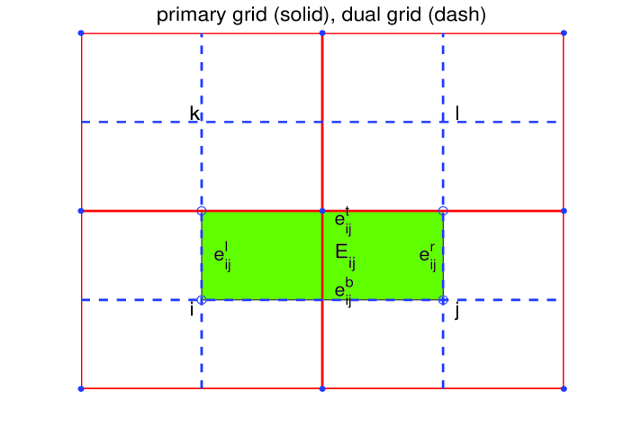
Figure 3.2: Rectangle primary grid and dual grid

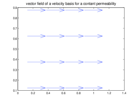
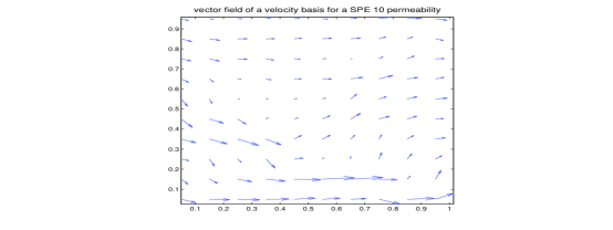
Figure 3.3: Vector field of a velocity basis function for homogeneous permeability (left) and vector field of a velocity basis function for heterogeneous permeability (right)

For many multiscale problems, in particular, the problems with separable scales, we can simply take $v(x)=(1,1)$. No global information is used in this case, we call this case the local multiscale method. If the permeability $k$ has strong long range features (e.g., highly channelized), we can use some global information $v(x)$ related to the features of $u$, e.g., the single-phase velocity at time zero, to construct the velocity multiscale basis functions [1]. In general, global information used to construct the basis functions in highly heterogeneous permeability often yields much better approximation than a constant boundary condition. Many numerical studies [1, 21] show the global information is very helpful to improve accuracy when the permeability $k$ has distinguished long range features. We note that one can use time-dependent global fields to construct multiscale basis functions. This is helpful for compressible flow simulations.

If multiple global fields $v_{n}(x)$ ($n=1,\cdots,N$) are used to build basis functions, then each interface corresponds to multiple multiscale basis functions $\phi_{ij}^{n}$ ($n=1,\cdots,N$), which solve

$$\begin{cases}\begin{split}-\text{div}(k\nabla\phi_{ij}^{n})&=0\ \ \text{in}\ \ \Omega_{ij},\\ -k\nabla\phi_{ij}^{n}\cdot n&=\left\{\begin{array}[]{ll}-\frac{v_{n}(x)\cdot n}{\int_{e_{ij}^{l}}v_{n}(x)\cdot ndx}&\text{on}\ \ e_{ij}^{l}\\ \frac{v_{n}(x)\cdot n}{\int_{e_{ij}^{l}}v_{n}(x)\cdot ndx}&\text{on}\ \ e_{ij}^{r}\\ 0&\text{on}\ \ e_{ij}^{b}\cup e_{ij}^{t}.\end{array}\right.\end{split}\end{cases}$$ (3.12)

We note that the multiple global fields $v_{n}(x)$ can be associated to some representative realizations in the setting of stochastic two-phase flows [22].

Remark 3.1.

By the result of Owhadi and Zhang [28], we can use $d$ ($d=dim(\Omega)$) global fields in (3.12). From the result, the global field $v_{n}(x)=-k\nabla p_{n}$ ($n=1,\cdots,d$) are the solutions of the elliptic equations

$$\begin{cases}\begin{split}-\text{div}(k\nabla p_{n})&=0\ \ \text{in}\ \ \Omega\\ p_{n}&=x_{n}\ \ \text{on}\ \ \partial\Omega,\end{split}\end{cases}$$ (3.13)

where $x=(x_{1},\cdots,x_{d})$.

Following the ideas in [21], the global information can be computed on an intermediate coarse grid using upscaling techniques. This will reduce the computation for the global information.

Because the source term of the basis equation (3.11) is zero, the flux conservation implies the following proposition.

Proposition 3.1.

Let $E_{ij}\in\mathcal{E}_{H}$ be any interface and $\psi_{ij}$ be the corresponding velocity basis function. Then

$$\int_{E_{ij}}\psi_{ij}\cdot n_{E_{ij}}dx=1.$$

Moreover, all $\psi_{ij}$ are linear independent, i.e., they form a set of finite element basis functions.

Remark 3.2.

If $k$ is a constant in $\Omega_{ij}$ and no global information is used, then $\psi_{ij}$ and $\psi_{ik}$ are orthogonal each other, i.e., the velocity basis function producing horizontal flux is orthogonal to the velocity basis function producing vertical flux. In fact, we can show that (see [25])

$$\psi_{ij}=\left\{\begin{array}[]{ll}{1\over|E_{ij}|}(1,0)&\ \ \text{on}\ \ \Omega_{ij}\\ 0&\ \ \text{else}\end{array}\right.\ \ \text{and}\ \ \psi_{ik}=\left\{\begin{array}[]{ll}{1\over|E_{ik}|}(0,1)&\ \ \text{on}\ \ \Omega_{ik}\\ 0&\ \ \text{else}\end{array}\right..$$

This coincides with the velocity basis in Example 1. If $k$ is varied in the coarse block, then $\psi_{ij}$ and $\psi_{ik}$ may not be orthogonal to each other any more. This can be observed from Figure 3.3 (right).

3.2 Analysis of the mixed MsFV

In this subsection we will show that the new mixed MsFV method is well defined. We have to check the conditions (2). The first one is straightforward since $\mathcal{P}_{H}=\mathcal{Q}_{h}$ and $\mathcal{U}_{H}=\mathcal{V}_{H}$. The second condition is verified below. We also give more details how to organize the computations.

The mixed finite volume formulation (3.8) implies the following algebraic linear system

$$\begin{cases}\begin{split}\mathbf{A}U+\mathbf{B}P&=0\\ \mathbf{C}U&=F,\end{split}\end{cases}$$ (3.14)

where $\mathbf{A}$ is a mass matrix. Here $\mathbf{B}$ has only nonzero entries $1$ and $-1$ and the $\mathbf{B}P$ represents the jump of $P$. The matrix $\mathbf{C}$ has only nonzero entries $1$ and $-1$, and the sign depends upon the normal direction to which the corresponding flux entries of $U$ associate. Because the first equation in (3.8) can be computed dual coarse block by dual coarse block and the support of velocity basis function lies in a dual coarse block, $\mathbf{A}$ can be represented as a block diagonal matrix, i.e., $\mathbf{A}=diag(A_{1},A_{2},\cdots)$, where each diagonal block $A_{i}$ is the mass matrix associated to a dual coarse block.

A straightforward calculation implies the following proposition.

Proposition 3.2.

Let $\mathbf{B}$ and $\mathbf{C}$ be defined in (3.14). Then $\mathbf{B}^{T}=\mathbf{C}$.

Because the mass matrix $\mathbf{A}$ is block diagonal in the mixed MsFV, this allows to invert each block entry $A_{1},A_{2},\cdots$ to eliminate the flux $U$ and the computation (for $A_{1}^{-1},A_{2}^{-1},\cdots$) is fast. It is known that mixed MsFEM also yields a system such as (3.14), but mass matrix in mixed MsFEM is not block diagonal and one has to globally compute the inverse of the mass matrix to eliminate the flux $U$. In general, the computation for the inverse in mixed FEM is quite time-consuming when the mass matrix is large. This is an advantage of mixed MsFV over mixed MsFEM. Figure 3.4 shows the mass matrix for $RT_{0}$ mixed FEM (left) and mixed MsFEM (right), respectively, where $6\times 10$ grid is used for both and permeability is heterogeneous (portion of SPE 10 in layer 85).

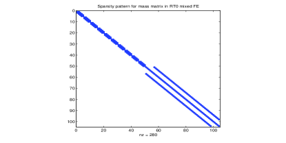
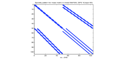
Figure 3.4: Sparsity patterns for mass matrix in lowest order Raviart-Thomas mixed FEM (left) and sparsity patterns for mass matrix in mixed MsFEM (right)

We analyze the block diagonal entries of $\mathbf{A}$. Let $D_{ijkl}$ be the control volume with vertexes $i,j,k,l$. In $D_{ijkl}$, $u_{H}$ can be represented by

$$u_{H}|_{D_{ijkl}}=u_{ij}\psi_{ij}+u_{ik}\psi_{ik}+u_{jl}\psi_{jl}+u_{kl}\psi_{kl}.$$

Consequently, the first equation in (3.8) can be reduced to be in $D_{ijkl}$

$$\begin{matrix}\begin{bmatrix}a_{ij,ij}&a_{ik,ij}&a_{jl,ij}&a_{kl,ij}\\ a_{ij,ik}&a_{ik,ik}&a_{jl,ik}&a_{kl,ik}\\ a_{ij,jl}&a_{ik,jl}&a_{jl,jl}&a_{kl,jl}\\ a_{ij,kl}&a_{ik,kl}&a_{jl,kl}&a_{kl,kl}\end{bmatrix}\begin{bmatrix}u_{ij}\\ u_{ik}\\ u_{jl}\\ u_{kl}\end{bmatrix}+\begin{bmatrix}p_{j}-p_{i}\\ p_{k}-p_{i}\\ p_{l}-p_{j}\\ p_{l}-p_{k}\end{bmatrix}=\begin{bmatrix}0\\ 0\\ 0\\ 0\end{bmatrix},\end{matrix}$$ (3.15)

where $a_{ik,ij}:=\int_{D_{ijkl}}k^{-1}\psi_{ij}\cdot\psi_{ik}dx$ and the other entries are defined similarly. We define $A$ to be the most left matrix in (3.15) and it is a symmetric and positive Gram matrix. We would like to note that $A$ is a representative for the diagonal entries in $\mathbf{A}$ defined in (3.14). We compute each multiscale basis functions $\psi_{ij}$ in fine scale by standard mixed FEM (e.g., Raviart-Thomas mixed FEM). Then $\psi_{ij}$ in $D_{ijkl}$ can be represented as $\psi_{ij}=\sum_{m}r_{ij,m}\psi^{h}_{m}$, where $\psi^{h}_{m}$ are standard mixed finite element basis functions in fine scale. Hence $A$ can be computed in the following way.

Proposition 3.3.

Let $A^{h}$ be the Gram matrix with entries $(A^{h})_{mn}=\int_{D_{ijkl}}k^{-1}\psi^{h}_{m}\cdot\psi^{h}_{n}dx$, and each column of $R$ consist of all $r_{ij,m}$. Then

$$A=R^{T}A^{h}R.$$

In particular, if permeability $k$ is homogeneous (constant) in a dual coarse block and the mesh is uniformly square and no global information is used, then a straightforward calculation implies that the corresponding matrix

$$A=diag(2,2,2,2),$$

i.e., $A$ is a diagonal matrix with diagonal entry 2.

Because $A$ is positive (or invertible), equation (3.15) implies that

$$\begin{matrix}\begin{bmatrix}u_{ij}\\ u_{ik}\\ u_{jl}\\ u_{kl}\end{bmatrix}=A^{-1}\begin{bmatrix}p_{i}-p_{j}\\ p_{i}-p_{k}\\ p_{j}-p_{l}\\ p_{k}-p_{l}\end{bmatrix}.\end{matrix}$$ (3.16)

Here $A^{-1}$ is a transmissibility matrix. We plug the expression (3.16) into the second equation in (3.8) to obtain a system about the pressure,

$$\mathbf{D}P=F.$$ (3.17)

Here $\mathbf{D}=\mathbf{C}\mathbf{A}^{-1}\mathbf{B}$, where $\mathbf{B}$ and $\mathbf{C}$ are defined in (3.14). We can show that $\mathbf{D}$ is sparse. In fact, from Equation (3.8), we know that only the fluxes of the interfaces of coarse volume $K_{i}$ contribute the mass conservation at volume $K_{i}$, and that each interface flux is determined by its neighbor pressures. Consequently, there are at most 9 nonzero entries for each row of matrix $\mathbf{D}$ for $2D$ rectangle cells. If we do not consider the restrictions of boundary condition, $\mathbf{D}$ is symmetric. This can be shown by using the fact $\mathbf{B}^{T}=\mathbf{C}$. Our numerical studies show that $\mathbf{D}$ is positive. When permeability is homogeneous, a rigorous mathematics proof for the positiveness can be found in [25]. Hence equation (3.17) is solvable. Once we obtain the pressure values, then we go back to equation (3.16) to get the flux vector $U$.

In particular, if the permeability $k$ is a constant, the scheme in (3.8) coincides with the standard cell-centered difference scheme. In this case, we get the following matrix $\tilde{\mathbf{D}}$ for a $2D$ uniformly square $3\times 3$ grid,

$$\begin{matrix}\tilde{\mathbf{D}}=\begin{bmatrix}2&-1&0&-1&0&0&0&0&0\\ -1&3&-1&0&-1&0&0&0&0\\ 0&-1&2&0&0&-1&0&0&0\\ -1&0&0&3&-1&0&-1&0&0\\ 0&-1&0&-1&4&-1&0&-1&0\\ 0&0&-1&0&-1&3&0&0&-1\\ 0&0&0&-1&0&0&2&-1&0\\ 0&0&0&0&-1&0&-1&3&-1\\ 0&0&0&0&0&-1&0&-1&2\end{bmatrix}.\end{matrix}$$ (3.18)

Here we assume Neumann boundary condition without restriction $\int_{\Omega}pdx=0$. If we restrict $\int_{\Omega}pdx=0$ for a unique solution, e.g., replace the fifth row in $\tilde{\mathbf{D}}$ by $(1,1,1,1,1,1,1,1,1)$, the matrix $\tilde{\mathbf{D}}$ becomes an invertible matrix $\mathbf{D}$.

We summarize the computation as following.
Algorithm 1

• For each interface $E_{ij}$, we solve basis equation (3.11).

• By equation (3.8), we formulate an algebraic system (3.14).

• Eliminate $U$ by local systems (3.15) and obtain equation (3.17).

• Solve equation (3.17) to get pressure $P$ and return to equation (3.16) to get $U$.

• By basis equation (3.11) and $U$, downscale coarse scale velocity to fine scale velocity.

3.3 Reconstruction of the fine-scale velocity field

Fluxes across the interfaces of primary coarse grid can be accurately computed by (3.16). In many situations it is often needed to accurately compute the small-scale velocities (or fluxes) in regions of interest. Although we can obtain the velocity in fine grid by straightforwardly prolonging the multiscale basis function into fine grid, the velocity are in general discontinuous on the interfaces of the dual coarse grid. Then large errors can occur in the divergence field and local mass balance is violated. We can use a post-procedure to reconstruct a conservative fine-scale velocity which is continuous on the interfaces of both fine grid and coarse grid and fully consistent with the fluxes across the coarse grid interfaces given by the velocity multiscale basis functions. We would like to note that a similar post-procedure is used in MsFV [20]. We describe the post-procedure as following.
Algorithm 2

• Extract the velocities through the interfaces of all coarse primary cells $K\in\mathcal{T}_{H}$. Let $u_{H}|_{\partial K}$ be the velocity across $\partial K$, the boundary of $K$.
  

• On each coarse grid $K$, the following local problem is solved by mixed finite element methods (or fine volume methods),

  $$\begin{cases}\begin{split}-\text{div}(k\nabla\tilde{p})&=f\ \ \text{in}\ \ K\\ -k\nabla\tilde{p}\cdot n&=u_{H}|_{\partial K}\cdot n\ \ \text{on}\ \ \partial K.\end{split}\end{cases}$$ (3.19)

• Define $\tilde{u}_{H}=\bigoplus_{K}\tilde{u}_{H}^{K}$, where $\tilde{u}_{H}^{K}=-k\nabla\tilde{p}$ and $\tilde{p}$ solves (3.19).

By the post-procedure, $\tilde{u}_{H}\in H(div,\Omega)$, that is to say, $\tilde{u}_{H}$ is continuous along all fine interfaces and coarse interfaces.

Remark 3.3.

Because there may exist some errors while computing $u_{H}$, $\int_{\partial K}u_{H}\cdot ndx$ may be not close to $\int_{K}fdx$ sufficiently. We can replace the source term $f$ in (3.19) by ${1\over|K|}\int_{\partial K}u_{H}\cdot ndx$ to remedy the little disparity for better accuracy.

Remark 3.4.

It the solution of problem (3.19) is considered to be computationally expensive, another set of basis functions could be constructed only once and used during the simulation (see [20] for a similar approach and [27] for details).

4 More mixed finite volume methods and their multiscale analogues

If we define different grids, approximation spaces or operators $\nabla_{h}$ and $\text{div}_{h}$, then we can obtain different mixed finite volume methods. One mixed finite volume method has already been described in Example 1 of Section 2, and its multiscale analogue has been developed and analyzed in Section 3. In this section, we briefly present more examples of mixed finite volume methods and their multiscale analogues.

The following Example 2 is closely related to Example 1.

Example 2 (Mixed FV 2).

The primary grid $\mathcal{T}_{h}$ and the dual mesh $\mathcal{D}_{h}$ are identical to the ones in Example 1. The discrete space $\mathcal{P}_{h}$ for pressure is the space of bilinear functions. The basis function of $\mathcal{P}_{h}$ for each cell center is one in the particular cell center and zero in all neighbors. $\mathcal{Q}_{h}$ is the space of piecewise constants on the primary grid. The approximation space for the vector variable, $\mathcal{U}_{h}=\mathcal{V}_{h}$ is the same as in Example 1 and $\nabla_{h}=\nabla$.

Unstructured grid is often used in practical simulations and mixed finite volume method can apply to the unstructured grid (see [13] for extensive discussions). The following example describe a mixed finite volume method on an unstructured grid.

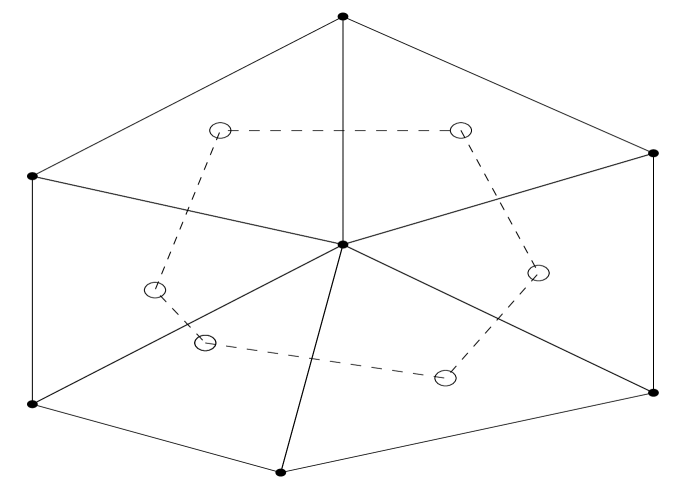
Figure 4.5: Voronoi box/Delaunay triangles

Figure 4.6: Triangle $D$

Example 3 (Mixed FV 3).

We assume that the dual grid $\mathcal{D}_{h}$ consists of triangles and the cells in the primary mesh $\mathcal{T}_{h}$ are control volumes around each vertex in $\mathcal{D}_{h}$. Particular example is the Delauney mesh as a dual grid and the corresponding Voronoi grid as primary grid (see Figure 4.5). The space $\mathcal{P}_{h}$ is the space of piece-wise linear functions on the dual grid. The space $\mathcal{Q}_{h}$ is the space of piece-wise constants on the primary grid. The approximation space for the vector variable, $\mathcal{U}_{h}=\mathcal{V}_{h}$, is the space of piece-wise constant vectors with continuous normal components and it is defined on the dual mesh (see Figure 4.6). The construction of the basis is analogous with the procedure described in Example 1. The operator $\nabla_{h}=\nabla$. Note that the dual grid can be any mesh of triangles, and the primary grid can consists of control volumes, not necessarily convex polygons, around each vertex. Frequently the control volumes are formed by connecting the middle of the edges of each triangle with the center of mass of the triangle. The details of the method can be found in [26].

If the dual grid is Delauney mesh and the primary grid is Voronoi mesh, then we can approximate the scalar variable with piecewise constants, i.e., $\mathcal{P}_{h}$ is the space of piecewise constants on the primary grid. Then the operator $\nabla_{h}$ is defined by (2.6).

Here we consider a mixed finite volume method closely related to the multi-point flux approximation (MPFA) discretizations [24].

Figure 4.7: Qaudrilateral mesh with volumes and covolumes

Figure 4.8: Quadrilateral $V_{i}$

Example 4 (Mixed FV 4).

The primary mesh is a general quadrilateral mesh (see Fig. 4.7). The dual cells are formed by connecting the cell-centers with the centers of the edges of the quadrilaterals. These lines split each primary cell $V_{i}$ into four quadrilaterals $V_{i,j},\,j=1,\,2,\,3,\,4$. The space $\mathcal{P}_{h}$ is the space of piecewise linear functions on $V_{i,j}$ with a common point in the cell center and the other two points on the edges on the quadrilateral $V_{i,j}$. (See Fig. 4.8). The space $\mathcal{Q}_{h}$ is the space of piecewise constant functions on the primary grid. The space $\mathcal{U}_{h}$ is the space of piecewise vector constants with continuous normals on the dual cells, and the space $\mathcal{V}_{h}$ is the space of piecewise vector constants on the dual cells. Note that these two spaces have different dimensions. Each local subspace $\mathcal{U}_{h,i}$ has four degrees of freedom. Each local subspace $\mathcal{V}_{h,i}$ has eight degrees of freedom. The operator $\nabla_{h}$ is defined by

$$\int_{\Omega}\nabla_{h}p_{h}\cdot v_{h}\,dx=\sum_{V_{i}\in\mathcal{T}_{h}}\sum_{j=1}^{4}\int_{V_{i,j}}\nabla p_{h}\cdot v_{h}\,dx.$$

Note that $\mathcal{P}_{h}$ here is not subspace of $H^{1}(\Omega)$. The approximation of $\nabla p$ is nonconforming. One way to make the mixed finite volume method more robust is to use a conforming approximation. For example, it is possible to use as $\mathcal{P}_{h}$ the space of piecewise bilinear functions on $V_{i,j}$. One extra basis function is added for each intersection of four adjoint primary cells in two dimensions [9]. Extra basis functions are required for three dimensional grids [17].

We note that the same procedure works for the grids in Example 3 [32].

We used the mixed finite volume methodology to develop a new mixed multiscale method based on Example 1 in Section 3. We will sketch how we can follow the same procedure and derive mixed multiscale finite volume methods based on Example 2 - Example 4. Some of the methods derived following this framework are known, most are new.

We assume that a consistent mixed finite volume method is defined on the fine mesh, i.e., fine primary and dual grids are given with the corresponding spaces and the operators. We need coarse primal and dual grids and we will assume that each coarse cell consists of fine cell of the same type, i.e., every coarse primary grid cell is a union of adjacent fine primary grid cells. The same is true for each coarse dual grid cell. This construction is straightforward for the structured grids. We suppose that an appropriate coarsening algorithm is used to define the coarse grid for the unstructured grids. The next step is to define the approximation spaces. We will require that the coarse discrete spaces provide some approximation of the corresponding functions. This requirement is easily fulfilled if we follow the same procedure on the coarse structured grids. For example the space $\mathcal{P}_{H}$ can consists of constant functions on the primary coarse grid $\mathcal{T}_{H}$. Then the space $\mathcal{U}_{H}$ has to be a multiscale space. We can consider a multiscale finite element (e.g., [14, 18, 20] for detailed description) space for $\mathcal{P}_{H}$ and the space $\mathcal{U}_{H}$ could be the space of piecewise constant vector functions on the dual cells. The situation is more complicated for unstructured grids. We need approximation of the gradient of the pressure on unstructured grids and therefore we have to use a multiscale finite element space $\mathcal{P}_{H}$. The space $\mathcal{U}_{H}$ can be either a standard piecewise vector constant space or a multiscale space.

We provide below more details for several mixed multiscale methods that can be derived following our methodology and using the mixed finite volume methods on the fine grid in Examples 2 - Example 4.

For better presentation, we call the mixed MsFV proposed in Section 3 to be Mixed MsFV 1.

Example 5 (Mixed MsFV 2).

The derivation below is related to Example 2 (Mixed MsFV 2). The primary grid $\mathcal{T}_{H}$ and the dual mesh $\mathcal{D}_{H}$ are identical to the ones in Mixed MsFV 1 (Section 3). We chose $\mathcal{P}_{H}$ to be the space of multiscale functions. The space $\mathcal{U}_{h}=\mathcal{V}_{h}$ is the space of piecewise constant vector functions with continuous normals on the dual coarse grid. The operator $\nabla_{H}=\nabla$.

The basis of $\mathcal{P}_{H}$ on $\mathcal{T}_{H}$ can be calculated in the same way as in [20]. Then we will exactly reproduce the method proposed in [20]. We can derive a different method by using a different basis for $\mathcal{P}_{H}$. For example, the discrete harmonic basis [33, 14] can be constructed in a multilevel way, that is cheaper, and the computations can be performed using only the fine matrix.

Another method is derived if we select $\mathcal{P}_{H}$ to be the space of bilinear functions and $\mathcal{U}_{h}=\mathcal{V}_{h}$ to be a multiscale space defined in the same way as in Mixed MsFV1. The operator $\nabla_{H}=\nabla$.

The case for unstructured grids is more complicated. Here we sketch the derivation of a mixed MsFV for unstructured fine triangular grids.

Example 6 (Mixed MsFV 3).

We assume that the primary and dual grids $\mathcal{T}_{H}$, $\mathcal{D}_{H}$ are constructed from fine cells described in Example 3 (MFV 3) using an appropriate coarsening algorithm [33]. The first method we propose uses a multiscale space $\mathcal{P}_{H}$ of discrete harmonic functions discussed in previous example. The space $\mathcal{U}_{H}=\mathcal{V}_{H}$ is the space of constant vector functions with continuous normals. The operator $\nabla_{H}=\nabla$. Note that this method does not use global information.

We recommend using the multiscale space $\mathcal{U}_{H}=\mathcal{V}_{H}$ when it is beneficial to use some global information about the problem and this information can be transferred using the velocity. The basis functions for $\mathcal{U}_{H}$ are constructed in a similar way as on the rectangular grid. We modify the definition of the velocity basis function (3.11) as follows. Consider the triangle $D$ on Figure 4.6. The basis function corresponding to $l_{i}$ is the solution of the following boundary value problem:

$$\begin{cases}\begin{split}-div(k\nabla\phi_{ij})&=0\ \ \text{in}\ \ D_{i}\cup D_{j},\\ -k\nabla\phi_{ij}\cdot n&=\left\{\begin{array}[]{ll}-\frac{v(x)\cdot n}{\int_{e_{ik}}v(x)\cdot ndx}&\text{on}\ \ e_{ik}\\ \frac{v(x)\cdot n}{\int_{e_{jk}}v(x)\cdot ndx}&\text{on}\ \ e_{jk}\\ 0&\text{on}\ \ l_{k}\cup l_{j}\\ 0&\text{on}\ \ e_{ij}\cup e_{ji}.\end{array}\right.\end{split}\end{cases}$$ (4.20)

Again $\nabla_{H}=\nabla$.

Example 7 (Mixed MsFV 4).

There are several ways to construct multiscale MPFA methods. One approach is presented in [20]. This requires a construction of a multisclale space $\mathcal{P}_{H}$ and the standard spaces for $\mathcal{U}_{H}$ and $\mathcal{V}_{H}$. Another method with the ability to utilize the available global information can be constructed by using a multiscale space $\mathcal{P}_{H}$, not necessarily the same as in [20], and a multiscale spaces $\mathcal{U}_{H}$ and $\mathcal{V}_{H}$ defined in similar way as (4.20). There exists a third way for rectangular or quadrilateral grids, such that the edges of the coarse cells are straight lines. We can use the standard finite element space $\mathcal{P}_{H}$ and a multiscale space $\mathcal{U}_{H}$. The framework also can be applied to the MPFA discretizations proposed in [9, 17, 32] and the corresponding mixed MsFV methods derived.

We note that it is difficult to apply standard multiscale basis functions in production code because of the geometric grid information necessary to impose the appropriate boundary conditions. It is also difficult to apply them for unstructured grids. If the coarse grid is very distorted, it may happen that a point where the four quadrilaterals meet is not in the support of the neighboring functions. This will decrease the accuracy. If discrete harmonic and multilevel basis is used, then computation becomes cheaper and can be applied on the matrix level (see [14]). The extensive study for these issues is still under investigation.

5 Numerical results

In this section, we apply the mixed MsFV propped in Section 3 to simulate incompressible two-phase flows in porous media. We will consider the porous media with non-separable scales and separable scales. In the first example, the permeability field is from SPE Comparative Solution Project [10] (also known as SPE 10) and its scales are non-separable, and it has channelized structure. In the second example, we consider the flows in two-point correlation permeability. The permeability is described with a two-point correlation function and has non-separable scales and distinct spatial variation. In the third example, the permeability is described by a periodic function with a small period and its scales are apparently separable. We apply the local mixed MsFV and global mixed MsFV to the flows in the three types of permeability fields. We will find that the mixed MsFV can provide accurate approximation on coarse grid and that using global information is able to greatly improve accuracy for the cases of non-separable scales.

In our numerical simulations, we will perform two-phase flow and transport simulations. The equations are given (in the absence of gravity and capillary effects) by flow equations

$$\text{div}(\lambda(S){k}\nabla p)=f,$$ (5.21)

where the total mobility $\lambda(S)$ is given by $\lambda(S)=\lambda_{w}(S)+\lambda_{o}(S)$ and $f$ is a source term. Here, $\lambda_{w}(S)=k_{rw}(S)/\mu_{w}$ and $\lambda_{o}(S)=k_{ro}(S)/\mu_{o}$ where $\mu_{o}$ and $\mu_{w}$ are viscosities of oil and water phases, correspondingly, and $k_{rw}(S)$ and $k_{ro}(S)$ are relative permeability of oil and water phases, correspondingly. The saturation is governed by

$${\partial S\over\partial t}+\text{div}({F})=0,$$ (5.22)

where ${F}={v}f_{w}(S)$, with $f_{w}(S)$, the fractional flow of water, given by $f_{w}=\lambda_{w}/(\lambda_{w}+\lambda_{o})$, and the total velocity ${v}$ by:

$${v}={v}_{w}+{v}_{o}=-\lambda(S){k}\nabla p.$$ (5.23)

In our simulations, we take $k_{rw}(S)=S^{2}$ and $k_{ro}(S)=(1-S)^{2}$. In the presence of capillary effects, an additional diffusion term is present in (5.22) and an efficient treatment of capillarity is proposed in [23]. We note that the porosity is 1 in the saturation equation (5.22).

We solve the two-phase flow system (5.21) and (5.22) by the classical IMPES (implicit pressure and explicit saturation). The saturation equation (5.22) is discretized in fine grid by upwind finite volume method. The temporal discretisation is an implicit scheme, which is unconditionally stable but produce a nonlinear system (Newton-Raphson iteration solves the nonlinear system). For completeness, we describe the upwind finite volume method for equation (5.22) in Appendix A.

We compare the saturation fields and water-cut data as a function of pore volume injected (PVI). The water-cut is defined as the fraction of water in the produced fluid and is given by $q_{w}/q_{t}$, where $q_{t}=q_{o}+q_{w}$, with $q_{o}$ and $q_{w}$ being the flow rates of oil and water at the production edge of the model. In particular, $q_{w}=\int_{\partial\Omega^{out}}f(S){v}\cdot{n}ds$, $q_{t}=\int_{\partial\Omega^{out}}{v}\cdot{n}ds$, where ${\partial\Omega^{out}}$ is the outer flow boundary. Pore volume injected, defined as $PVI={1\over V_{p}}\int_{0}^{t}q_{t}(\tau)d\tau$, with $V_{p}$ being the total pore volume of the system, provides the dimensionless time for the displacement. We consider a traditional quarter five-spot problem, where the water is injected at left bottom corner and oil is produced at the right top corner of the rectangular domain. In all numerical simulations, multiscale basis functions are constructed once at the beginning of the computations. In the discussions, we refer to the grid where multiscale basis functions are constructed as a coarse grid. We use the global single-phase information (where $\lambda(S)=1$) to construct mixed MsFV basis functions. The global information is computed on fine grid at time zero and will not change throughout the simulation.

In the simulations, we solve the pressure equation on the coarse grid by Algorithm 1 and use the post-procedure described in Algorithm 2 to re-construct the fine-scale velocity field which is used to solve the saturation equation.

We solve the two-phase pressure equation (5.21) by the mixed MsFV (mixed FEM for reference solution). For the numerical simulations, we use 10 time steps for pressure equation, and for each pressure time step, we use 10 time steps to solve saturation equation. Hence, the time step for pressure is 0.1 PVI and the time step for saturation is 0.01 PVI.

To assess the performance of the saturations and water-cuts obtained using the mixed MsFV, we compute the time-dependent pressure equation on fine grid by using lowest order Raviart-Thomas mixed finite element method, and this produces a reference velocity to solve a reference saturation solution $S_{ref}$. By the reference saturation and the reference velocity, we get the reference water-cut $W_{ref}$. We measure the relative saturation error in $L^{1}$-norm and the relative water-cut error in $L^{2}$-norm,

$$\|S_{MsFV}-S_{ref}\|_{L^{1}}/\|S_{ref}\|_{L^{1}},\quad\|W_{MsFV}-W_{ref}\|_{L^{2}}/\|W_{ref}\|_{L^{2}}.$$

where $S_{MsFV}$ and $W_{MsFV}$ denote the saturation and water-cut by the mixed MsFV, respectively.

5.1 Flow in SPE 10 permeability

For the first numerical example, we choose the SPE 10 permeability (layer 85), which is highly channelized and defined on a $60\times 220$ find grid. The permeability map is depicted in Figure 5.9. We take $3\times 5$ coarse grid for both the global mixed MsFV and the local mixed MsFV. We take tests for two different viscosity ratios of water and oil.

For the first test of the example, we consider the case that viscosity ratio $\mu_{w}/\mu_{o}$ of water and oil is less than 1. Here we take $\mu_{w}/\mu_{o}=1/10$ for the simulation. Figure 5.10 shows the reference (fine-scale) saturation profile, the saturation profile using the global mixed MsFV and the saturation profile using the local mixed MsFV, respectively, at PV1=1. Figure 5.11 shows the saturation error via different PVI times. From the figure, we find that the mixed MsFV using global information render more accurate saturation solutions throughout the whole simulation than the saturation from the local mixed MsFV. The water-cut curves are shown in Figure 5.12 for reference, global mixed MsFV and local mixed MsFV, respectively. The water break-through time is almost the same for the three methods, however, the water-cut curve by using global mixed MsFV is closer to the reference water-cut curve at early time than the local mixed MsFV. The average errors of saturation and water-cut are shown in Table 1. We observe that the error of the solution of the global mixed MsFV is at least two times smaller than the error of the solution of the local MsFV.

For the second test of the example, we consider the case when $\mu_{w}/\mu_{o}=3$. Figure 5.13 depicts the reference saturation profile and the saturation profiles uisng both the global mixed MsFV and the local mixed MsFV at PV1=1. Figure 5.14 illustrates the saturation error via different PVI times and the water-cut curves as well. From Figure 5.13 and Figure 5.14, we find that global mixed MsFV performs better than local mixed MsFV in the point of view of accuracy and water-breakthrough time. Table 1 shows the average errors of saturation and water-cut for the test.

Figure 5.9: Logarithm of SPE 10 permeability, layer 85.

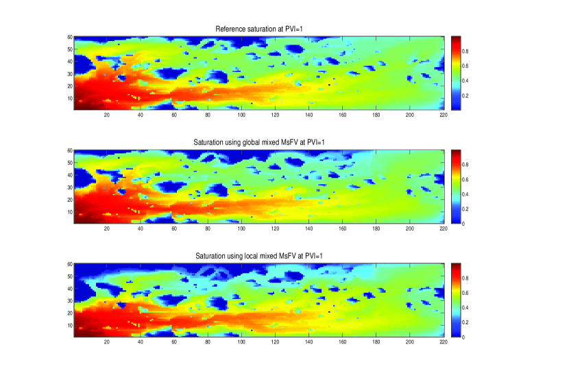
Figure 5.10: Saturation profiles, $\mu_{w}/\mu_{0}=1/10$. Top: Reference saturation at PVI=1. Middle: Saturation at PVI=1 by the global mixed MsFV. Bottom: Saturation at PVI=1 by the local mixed MsFV.

Figure 5.11: saturation error via time, $\mu_{w}/\mu_{0}=1/10$.

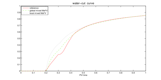
Figure 5.12: water-cut curves, $\mu_{w}/\mu_{0}=1/10$.

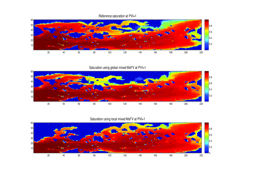
Figure 5.13: Saturation profiles, $\mu_{w}/\mu_{0}=3$. Top: Reference saturation at PVI=1 . Middle: Saturation at PVI=1 by the global mixed MsFV. Bottom: Saturation at PVI=1 by the local mixed MsFV.

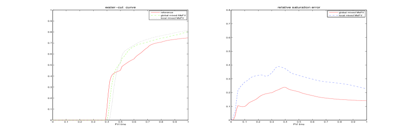
Figure 5.14: water-cut curves and saturation error via time, $\mu_{w}/\mu_{0}=3$.

Table 1: relative errors for saturation and water-cut, $\mu_{w}/\mu_{0}=1/10$

mixed MsFV	Water-Cut Error	Saturation Error
local mixed MsFV	0.1140	0.2024
global mixed MsFV	0.0510	0.0870

Table 2: relative errors for saturation and water-cut, $\mu_{w}/\mu_{0}=3$

mixed MsFV	Water-Cut Error	Saturation Error
local mixed MsFV	0.1748	0.2892
global mixed MsFV	0.1062	0.1535

5.2 Flow in two-point correlation permeability

In the second example, we choose a realization of the permeability field generated using a two-point correlation function with correlation lengths in $x_{1}$-direction $L_{1}=0.4$ and in $x_{2}$-direction $L_{2}=0.05$. Exponential variogram is selected (see e.g., [12]) to generate the permeability. The permeability is defined on $200\times 200$ fine-grid and depicted in Figure 5.15. The viscosity ratio is $\mu_{w}/\mu_{o}=1/3$ and the mixed MsFVs are implemented on $10\times 10$ coarse grid. Figure 5.16 depicts the reference saturation, the saturation field using the global mixed MsFV and the saturation field using the local mixed MsFV, respectively. Figure 5.17 demonstrate the relative saturation error via different PVI times. From the figure, we observe that mixed MsFV can provide a good approximation for the flow, and that using global information improves the accuracy. The water-cut curves are depicted in Figure 5.18 for reference, global mixed MsFV and local mixed MsFV, respectively. Figure 5.18 shows that the water-cut curve in global mixed MsFV is more close to the reference water-cut curve than the mixed MsFV without using global information, and that the water break-through time in global mixed MsFV is almost the same as the reference water break-through time. The average errors of saturation and water-cut are shown in Table 3. From Table 3, we can observe: the saturation in the global mixed MsFV is almost 9 times better than the saturation in the local mixed MsFV, and the water-cut in global mixed MsFV is around 3 times better than the water-cut in the local mixed MsFV.

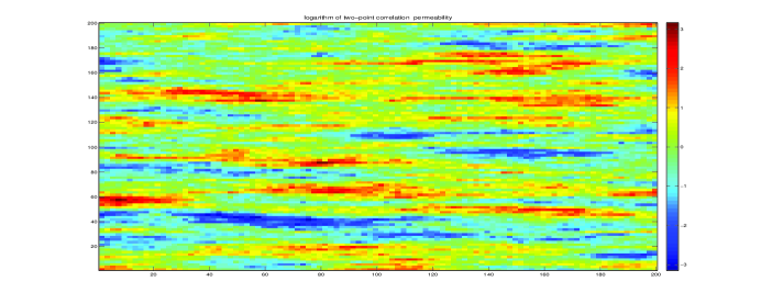
Figure 5.15: Logarithm of two-point correlation permeability

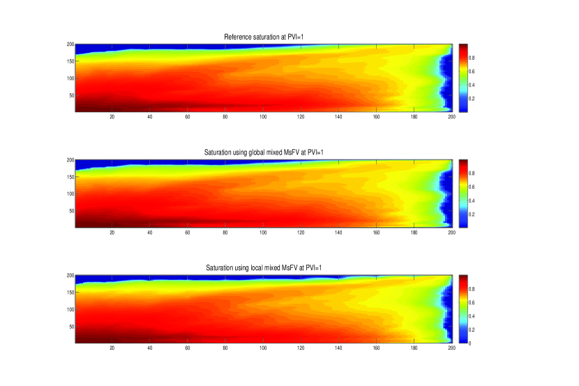
Figure 5.16: Top: Reference saturation at PVI=1 for the second example. Middle: Saturation at PVI=1 by the global mixed MsFV. Bottom: Saturation at PVI=1 by the local mixed MsFV.

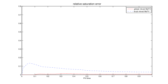
Figure 5.17: saturation error via time for the second example

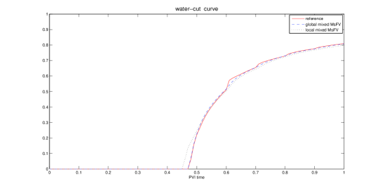
Figure 5.18: water-cut curves for the second example

Table 3: relative errors for saturation and water-cut for the second example

mixed MsFV	Water-Cut Error	Saturation Error
local mixed MsFV	0.0464	0.0610
global mixed MsFV	0.0127	0.0075

5.3 Flow in periodic permeability

In the third numerical example, we choose the permeability which is specified by a periodic function

$$k(x,y)=\frac{2+1.8\sin(2\pi x/\epsilon)}{2+1.8\sin(2\pi y/\epsilon)}+\frac{2+1.8\sin(2\pi y/\epsilon)}{2+1.8\cos(2\pi x/\epsilon)},\ \ \epsilon=1/25.$$

The permeability is defined on $100\times 100$ fine grid and its map is depicted in Figure 5.19. Figure 5.20 depicts the reference (fine-scale) saturation, the saturation using the global mixed MsFV and the saturation using the local mixed MsFV, respectively, at PVI=1. Here $5\times 5$ coarse grid is taken for simulation in both the global mixed MsFV and the local mixed MsFV and the viscosity ratio is $\mu_{w}/\mu_{o}=1/10$. Figure 5.20 shows that the saturation profile by global mixed MsFV is almost the same as the saturation profile by local mixed MsFV and both of them are pretty close to the reference saturation profile. The saturation error via different PVI times is shown in Figure 5.21. It can be seen that the two saturation errors are very close and quite small. The water-cut curves are shown in Figure 5.22 for reference, global mixed MsFV and local mixed MsFV, respectively. Figure 5.22 shows that the three water-cut curves coincides each other. The average errors of saturation and water-cut are shown in Table 4. We find from Table 4 that: (1) the average errors of saturation and water-cut by global mixed MsFV and local mixed MsFV are comparable. (2) the average errors of saturation are less than $1\%$ and the average errors of water-cut are less than $2\%$. This example shows that local mixed MsFV can provide very good accuracy in the case of separable scales (e.g., periodic) and its performance is as good as the global mixed MsFV. The example confirms the findings for many multiscale finite elements (e.g.,[3, 8, 21]).

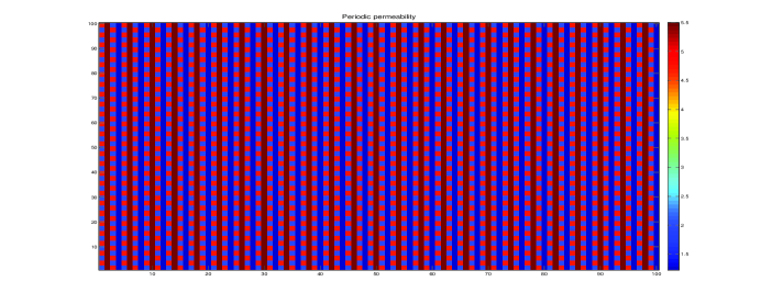
Figure 5.19: Periodic permeability

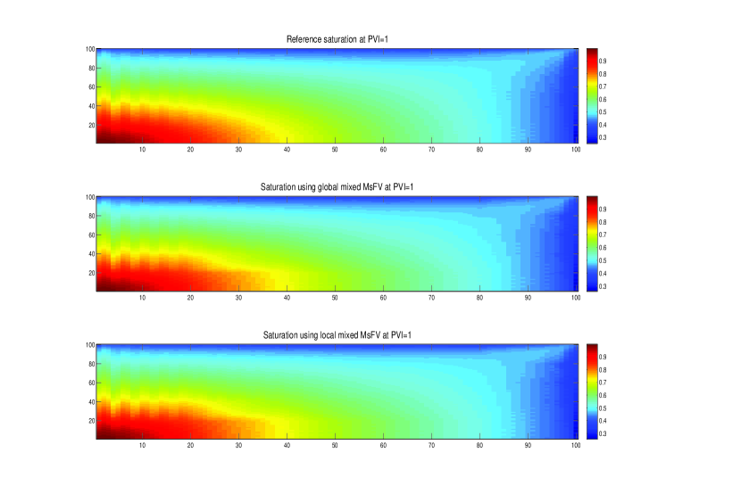
Figure 5.20: Top: Reference saturation at PVI=1 for the third example. Middle: Saturation at PVI=1 by the global mixed MsFV. Bottom: Saturation at PVI=1 by the local mixed MsFV.

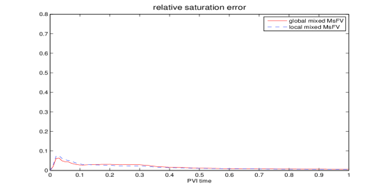
Figure 5.21: saturation error via time for the third example

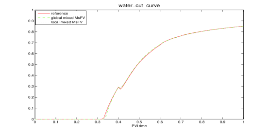
Figure 5.22: water-cut curves for the third example

Table 4: relative errors for saturation and water-cut for the third example

mixed MsFV	Water-Cut Error	Saturation Error
local mixed MsFV	0.0074	0.0171
global mixed MsFV	0.0082	0.0169

6 Conclusions

We developed a framework of mixed MsFV methods for elliptic equations arising from flows in porous media. These methods take advantages of both mixed MsFEM and finite volume methods. The essential characteristic of mixed MsFv is the explicit approximation of both pressure and velocity. We proposed a new multiscale basis functions for velocity. Global information can be used to construct the multiscale velocity basis functions to improve accuracy for highly heterogeneous porous media. We analyze one of the mixed MsFV methods and apply it to simulate two-phase flows in porous media. We test the method on permeability fields with both non-separable and separable scales. Numerical examples demonstrate that the mixed MsFV can efficiently approximate the two-phase flows on coarse grid. Using global information in the mixed MsFV yields much better accuracy than the local mixed MsFV if the permeability field has strong no-local features.

We also can use multiscale basis for the pressure. Discrete harmonic and energy minimizing basis constructed in a multilevel fashion is accurate and the computations are very efficient [33, 14]. Moreover, the methods easily can be extended to unstructured grids without requiring extra geometric information. Further investigation of these issues is worth pursuing in the future.

Appendix A Upwind finite volume method for Equation 5.22

In the Appendix, we would like to present a finite volume discretization of the saturation equation (5.22). Let $\gamma_{ij}$ be the common face (or edge) of $K_{i}^{h}$ (underlying fine grid) and $K_{j}^{h}$ (underlying find grid) and $n_{ij}$ be the normal vector pointing from $K_{i}^{h}$ to $K_{j}^{h}$. Using the $\theta$-rule for temporal discretization and a finite-volume scheme for the saturation equation, it follows the following form.

$$\frac{1}{\Delta t}(S_{i}^{n+1}-S_{i}^{n})+\frac{1}{|K_{i}^{h}|}\sum_{j\neq i}[\theta F_{ij}(S^{n+1})+(1-\theta)F_{ij}(S^{n})]=0,$$ (A.24)

where $S_{i}^{n}$ is the cell-average of water saturation at $t=t_{n}$, i.e.,

$$S_{i}^{n}=\langle S(x,t_{n})\rangle_{K_{i}^{h}}$$

and $F_{ij}$ is a numerical approximation of the flux over $\gamma_{ij}$, i.e.,

$$F_{ij}(S)\approx\int_{\gamma_{ij}}f_{w}(S)_{ij}u_{ij}\cdot n_{ij}ds.$$

Here $f_{w}(S)_{ij}$ denotes the fractional-flow function associated with $\gamma_{ij}$ and the first-order upstream weighting scheme for it is defined as

$$f_{w}(S)_{ij}=\left\{\begin{array}[]{ll}f_{w}(S_{i})&\mbox{if $u\cdot n_{ij}\geq 0$}\\ f_{w}(S_{j})&\mbox{if $u\cdot n_{ij}<0$.}\end{array}\right.$$

For $\theta=0$ or $1$, we can write (A.24) as a vector form

$$S^{n+1}=S^{n}+(\delta_{x}^{t})^{T}Af(S^{m}),\ \ m=n\ \ or\ \ n+1,$$

where $(\delta_{x}^{t})_{i}={\Delta t\over|K_{i}^{h}|}$.

If $\theta=0$, then (A.24) is an explicit scheme and only stable provided that time step $\Delta t$ satisfies a stability condition.

For $\theta=1$, (A.24) is an implicit scheme and unconditionally stable but gives rise to a nonlinear system. Such a nonlinear system is often solved with a Newton-Raphson iterative method. Define

$$G(S^{n+1})=S^{n+1}-S^{n}-(\delta_{x}^{t})^{T}Af(S^{n+1}).$$ (A.25)

By Taylor expansion, we have

$$G(S^{n+1})\approx G(S^{n})+G^{\prime}(S^{n})(S^{n+1}-S^{n}).$$

Noticing $G(S^{n+1})=0$ we have $\delta S^{n}:=S^{n+1}-S^{n}=-[G^{\prime}(S^{n})]^{-1}G(S^{n})$. From (A.25), we have

$$G^{\prime}(S)=I-(\delta_{x}^{t})^{T}Af^{\prime}(S),$$

where $f^{\prime}(S)_{i}=f^{\prime}(S_{i})$. Hence

$$S^{n+1}=S^{n}+\delta S^{n}.$$

This iteration proceeds until pre-defined iterations are reached or the norm of $\delta S^{n}$ is smaller than a prescribed value.

References

- [1] J. E. Aarnes, Y. Efendiev and L. Jiang, Mixed multiscale finite element methods using limited global information, Multiscale Modeling and Simulation, 7 (2008), pp. 655–676.
- [2] I. Aavatsmark, T. Barkve, O. Bøe, Discretization on unstructured grids for inhomogeneous, anisotropic media. Part I: Derivation of the methods, SIAM Journal on Scientific Computing, 19 (1998), pp. 1700–1716.
- [3] T. Arbogast, Implementation of a locally conservative numerical subgrid upscaling scheme for two-phase Darcy flow, Comput. Geosci., 6 (2002), pp. 453–481.
- [4] T. Arbogast, G. Pencheva, M. F. Wheeler, and I. Yotov, A multiscale mortar mixed finite element method, Multiscale Modeling and Simulation, 6 (2007), pp. 319-346.
- [5] I. Babuka and E. Osborn, Generalized finite element methods: Their performance and their relation to mixed methods, SIAM J. Numer. Anal., 20 (1983), pp. 510–536.
- [6] F. Brezzi, Interacting with the subgrid world, in Numerical analysis 1999 (Dundee), Chapman & Hall/CRC, Boca Raton, FL, 2000, pp. 69–82.
- [7] F. Brezzi and M. Fortin, Mixed and hybrid finite element methods, 1991, Springer–Verlag, New York.
- [8] Z. Chen and T. Y. Hou, A mixed multiscale finite element method for elliptic problems with oscillating coefficients, Math. Comp.,72(2003), pp. 541-576.
- [9] Q.-Y. Chen, J. Wan, Y. Yang, and R.T. Mifflin, Enriched Multi-Point Flux Approximation For General Grids, J. Comput. Phys., 227 (2008), pp. 1701-1721.
- [10] M. Christie and M. Blunt, Tenth SPE Comparative Solution Project: A comparison of upscaling techniques, SPE Reser. Eval. Eng., 4 (2001), pp. 308–317.
- [11] C. Dawson, S. Sun and M. F. Wheeler, Compatible algorithms for coupled flow and transport, Comput. Methods Appl. Mech. Engrg., 193 (2004), pp. 2565–2580.
- [12] C. Deutsch and A. Journel, GSLIB: Geostatistical software library and user’s guide, 2nd edition, Oxford University Press, New York, 1998.
- [13] J. Droniou and R. Eymard, A mixed finite volume scheme for anisotropic diffusion problems on any grid, Numerische Mathematik, 105 (2006), pp. 35–71.
- [14] O. Dubois, I. D. Mishev and L. Zikatanov, Energy minimizing bases for efficient multiscale modelling and linear solvers in reservoir simulation, Paper SPE-119137 presented at 20th SPE Reservoir Simulation Symposium, The Woodlands, Texas, 12-15 February 2009.
- [15] W. E and B. Engquist, The heterogeneous multi-scale methods, Comm. Math. Sci., 1(1) (2003), pp. 87–133.
- [16] M. G. Edwards and C. F. Roger, Finite volume discretization with imposed flux continuity for the general pressure equation, Comput. Geosci., 2 (1998), 259–290.
- [17] M. G. Edwards, H. Zheng, A quasi-positive family of continuous Darcy-flux finite-volume schemes with full pressure support, J. Comput. Phys., 227 (2008), pp. 9333-9364.
- [18] T. Y. Hou and X. H. Wu, A multiscale finite element method for elliptic problems in composite materials and porous media, J. Comput. Phys., 134 (1997), pp. 169–189.
- [19] T. Hughes, G. Feijoo, L. Mazzei, and J. Quincy, The variational multiscale method - a paradigm for computational mechanics, Comput. Methods Appl. Mech. Engrg, 166 (1998), pp. 3–24.
- [20] P. Jenny, S. H. Lee, and H. Tchelepi, Multi-scale finite volume method for elliptic problems in subsurface flow simulation, J. Comput. Phys., 187 (2003), pp. 47–67.
- [21] L. Jiang, Y. Efendiev and I. Mishev, Mixed multiscale finite element methods using approximate global information based on partial upscaling, Comput. Geosci., 14 (2010), pp. 319–341.
- [22] L. Jiang, I. Mishev and Y. Li, Stochastic mixed multiscale finite element methods and their applications in random porous media, Comput. Methods Appl. Mech. Engrg., 199 (2010), pp. 2721–2740.
- [23] J. Kou and S. Sun, A new treatment of capillarity to improve the stability of IMPES two-phase flow formulation, Computers and Fluids, 39 (2010), pp. 1923–1931.
- [24] I. Mishev, Nonconforming finite volume method, Comput. Geosci., 6 (2002), pp. 253–268.
- [25] I. Mishev, Analysis of a new mixed finite volume method, Computational Methods in Applied Mathematics, 3 (2003), pp. 189–201.
- [26] I. Mishev and Q. Y. Chen, A mixed finite volume method for elliptic problems, Numerical methods for PDE, 23 (2007), pp. 1122–1138.
- [27] I. Mishev, L. Jiang, and O. Dubois, Method and System for Finite Volume Simulation of Flow, U.S. Patent Application No. 61/330,012, filed April 30, 2010.
- [28] H. Owhadi and L. Zhang, Metric based up-scaling, Com. Pure Appl. Math., 60 (2007), pp. 675-723.
- [29] J. E. Roberts and J. M. Thomas, Mixed and hybrid methods, Handbook of Numerical Analysis 2, 1991, Elsevier Science Pub Co.
- [30] J.-M. Thomas and D. Trujillo, Mixed finite volume methods, Internat. J. Numer. Methods Engrg., 46 (1999), pp. 1351 -1366.
- [31] S. Sun and J. Geiser, Multiscale discontinuous Galerkin and operator-splitting methods for modeling subsurface flow and transport, International Journal for Multiscale Computational Engineering, 6 (2008), pp. 87–101.
- [32] S. K. Verma and K. Aziz, Two- and three-dimensional flexible grids for reservoir simulation, Proceedings of 5th European Conference on the Mathematics of Oil Recovery, Leoben, Austria, (1996).
- [33] J. Xu, L. Zikatanov, On an energy minimizing basis for algebraic multigrid methods, Comput. Visual. Sci., 7 (2004), pp. 21-127.