$1/(N-1)$ expansion based on a perturbation theory in $U$
for the Anderson model with $N$-fold degeneracy

Abstract

We study low-energy properties of the $N$-fold degenerate Anderson model. Using a scaling that takes $u=(N-1)U$ as an independent variable in place of the Coulomb interaction $U$, the perturbation series in $U$ is reorganized as an expansion in powers of $1/(N-1)$. We calculate the renormalized parameters, which characterize the Kondo state, to the next leading order in the $1/(N-1)$ expansion at half-filling. The results, especially the Wilson ratio, agree very closely with the exact numerical renormalization group results at $N=4$. This ensures the applicability of our approach to $N>4$, and we present highly reliable results for nonequilibrium Kondo transport through a quantum dot.

The Anderson impurity has been studied extensively as a model for strongly correlated electrons in dilute magnetic alloys, quantum dots, and also for bulk systems in conjunction with the dynamical mean-field theory Hewson_book . For quantum dots, the nonequilibrium Kondo effect can occur when a bias voltage is applied between two leads. A universal Fermi-liquid behavior Nozieres ; YY2 ; ZlaticHorvatic ; Yoshimori has been closely examined at low energies for the steady current Grobis ; ScottNatelson ; KNG ; ao2001 ; FujiiUeda ; HBA and shot noise Delattre ; GogolinKomnik ; Golub ; Sela2009 ; Mora2009 ; Fujii2010 .

Orbital degeneracy in the impurity states also affects the nonequilibrium properties at low energies. Recently, Mora et al. Mora2009 have succeeded to express the current noise in terms of the Fermi-liquid parameters Nozieres ; YY2 ; ZlaticHorvatic ; Yoshimori in an SU($N$) Kondo regime, where the Coulomb repulsion $U$ is so large that charge fluctuations are suppressed near the impurity with $N$-fold degeneracy. A complemental expression that takes into account the fluctuations at half-filling has been presented in our previous work Sakano . In this case, the corrections due to finite $U$ enter through the Wilson ratio $R$, which is a correlation function defined with respect to the equilibrium ground state, and through the width of the Kondo resonance $\widetilde{\Delta}$. Therefore, explicit values of these two parameters, $R$ and $\widetilde{\Delta}$, are required to study the low-energy transport thoroughly. The exact numerical renormalization group (NRG) approach is still applicable to multi-orbital systems. It practically works, however, for small degeneracies $N\leq 4$ Sakano ; Nishikawa1 , which for $N=2$ corresponds to the spin degeneracy. Therefore, alternative approaches are needed to explore the large degeneracies at $N>4$.

In this Letter, we propose a systematic approach to calculate correlation functions at $N>4$, using a scaling that takes $u=(N-1)U$ as an independent variable in place of $U$. Here, the factor $N-1$ corresponds to the number of different impurity states, with which a local electron in the impurity site can interact. With this scaling, the perturbation series in $U$ can be reorganized as an expansion in powers of $1/(N-1)$, using a diagrammatic classification similar to the one for the $N$-component $\varphi^{4}$ model WilsonKogut . However, our approach is completely different from the usual $1/N$ expansion and non-crossing approximation, which are constructed on the basis of the perturbation expansion in the hybridization matrix element $v_{\nu}$ Bickers ; Haule ; OtsukiKuramoto . We calculate $R$ and $\widetilde{\Delta}$ up to the next leading order terms in the $1/(N-1)$ expansion at half-filling, and find that the results agree very closely with the NRG results at $N=4$, where $N$ is still not so large. Particularly, the Wilson ratio shows an excellent agreement over the whole range of $U$. The early convergence of the expansion implies that our scaling procedure efficiently captures the orbital effects, and ensures the applicability to $N>4$. This enables us to present highly reliable results for the nonequilibrium steady current and shot noise for $N>4$. Our approach could have wide application to quantum impurities, and could be used as a solver for the dynamical mean-field theory DMFT .

The Hamiltonian for the $N$-fold degenerate Anderson model connected to two leads ($\nu=L,\,R$) is given by

$${\cal H}\,=\,{\cal H}_{0}+{\cal H}_{U},\qquad{\cal H}_{U}=\,\frac{1}{2}\sum_{m\neq m^{\prime}}U\,n_{dm}n_{dm^{\prime}},$$ (1)

$$\!{\cal H}_{0}=\sum_{\nu=L,R}\sum_{m=1}^{N}\int_{-D}^{D}\!d\epsilon\,\epsilon\,c^{\dagger}_{\epsilon\nu m}c_{\epsilon\nu m}+\sum_{m=1}^{N}\epsilon_{d}\,d_{m}^{\dagger}d_{m},$$

$$\quad\ +\sum_{\nu=L,R}\,\sum_{m=1}^{N}v_{\nu}\left(d_{m}^{\dagger}\psi_{\nu m}+\mbox{H.c.}\right).$$ (2)

Here, $d_{m}^{\dagger}$ creates an electron with energy $\epsilon_{d}$ in orbital $m$ at the impurity site, $n_{dm}=d_{m}^{\dagger}d_{m}$, and $m$ ($=1,2,\cdots,N$) includes the spin degrees of freedom. $c_{\epsilon\nu m}^{\dagger}$ creates a conduction electron with energy $\epsilon$ and orbital $m$ in lead $\nu$, and is normalized as $\{c^{\phantom{\dagger}}_{\epsilon\nu m},c^{\dagger}_{\epsilon^{\prime}\nu^{\prime}m^{\prime}}\}=\delta_{\nu\nu^{\prime}}\,\delta_{mm^{\prime}}\delta(\epsilon-\epsilon^{\prime})$. The linear combination $\psi_{\nu m}\equiv\int_{-D}^{D}d\epsilon\sqrt{\rho}\,c^{\phantom{\dagger}}_{\epsilon\nu m}$, with $\rho=1/(2D)$, couples to the impurity level via the hybridization matrix element $v_{\nu}$, and $\Delta\equiv\Gamma_{L}+\Gamma_{R}$ with $\Gamma_{\nu}=\pi\rho\,v_{\nu}^{2}$. We consider the parameter region where $\Delta$, $\epsilon_{d}$, and $U$ are much smaller than the half band width $D$.

We use the imaginary-frequency Green’s function that takes the form $G(i\omega)=\left[i\omega-\epsilon_{d}+i\Delta\,\mathrm{sgn}\,\omega-\Sigma(i\omega)\right]^{-1}$ for $|\omega|\ll D$. The behavior of the self-energy $\Sigma(i\omega)$ for small $\omega$ determines the enhancement factor for the linear specific heat $\widetilde{\gamma}=1-{\partial\Sigma(i\omega)}/{\partial(i\omega)}|_{\omega=0}$, and the renormalized parameters $z={1}/{\widetilde{\gamma}}$, $\,\widetilde{\epsilon}_{d}=z[\epsilon_{d}+\Sigma(0)]$, and $\widetilde{\Delta}=z\Delta$. The average number of local electrons can be deduced from the phase shift $\delta\equiv\cot^{-1}({\widetilde{\epsilon}_{d}}/{\widetilde{\Delta}})$, using the Friedel sum rule, $\langle n_{dm}\rangle=\delta/\pi$. The enhancement factor for the spin susceptibility and that for the charge can be written in the form $\widetilde{\chi}_{s}\equiv\widetilde{\chi}_{mm}-\widetilde{\chi}_{mm^{\prime}}$ and $\widetilde{\chi}_{c}\equiv\widetilde{\chi}_{mm}+(N-1)\,\widetilde{\chi}_{mm^{\prime}}$ for $m\neq m^{\prime}$. These susceptibilities can be deduced from the self-energy and four-point vertex function $\Gamma_{mm^{\prime};m^{\prime}m}(i\omega_{1},i\omega_{2};i\omega_{3},i\omega_{4})$ for $m\neq m^{\prime}$, using the Ward identities Yoshimori ,

$$\widetilde{\chi}_{mm}=\widetilde{\gamma},\quad\ \ \widetilde{\chi}_{mm^{\prime}}=-\,\frac{\sin^{2}\delta}{\pi\Delta}\,\Gamma_{mm^{\prime};m^{\prime}m}(0,0;0,0).$$ (3)

Furthermore, $\widetilde{U}\equiv z^{2}\Gamma_{mm^{\prime};m^{\prime}m}(0,0;0,0)$ corresponds to the residual interaction between the quasi-particles.

The Wilson ratio $R$ parameterizes how far the system is away from the Kondo limit, and plays a central role for finite $U$,

$$R\equiv\frac{\widetilde{\chi}_{s}}{\widetilde{\gamma}}=1+\frac{\widetilde{g}}{N-1}\,\sin^{2}\delta,\qquad\frac{\widetilde{\chi}_{c}}{\widetilde{\gamma}}=1-\widetilde{g}\sin^{2}\delta.$$ (4)

Here, the scaling factor $N-1$ is introduced to the renormalized interaction $\widetilde{U}$ and the bare one $U$, such that

$$\widetilde{g}\,\equiv\,(N-1)\,\frac{\widetilde{U}}{\pi\widetilde{\Delta}}\;,\qquad\quad g\,\equiv\,(N-1)\,\frac{U}{\pi\Delta}\;.$$ (5)

In the following we consider the particle-hole symmetric case, where $\epsilon_{d}=-(N-1)U/2$ and $\delta=\pi/2$. In this case, the renormalized coupling takes a value in the range $0\leq\widetilde{g}\leq 1$. It approaches to $\widetilde{g}\to 1$ in the limit of $g\to\infty$ as the charge fluctuation is suppressed $\widetilde{\chi}_{c}\to 0$.

We calculate $\widetilde{\gamma}$ and $\Gamma_{mm^{\prime};m^{\prime}m}(0,0;0,0)$ perturbatively to order $U^{3}$ and $U^{4}$, respectively, by extending Yamada’s calculations for $N=2$ YY2 to general $N$ Sakano , and obtain

$$\widetilde{g}\,= \ \ g-\frac{N-2}{N-1}\ g^{2}+\frac{(N-1)^{2}-\frac{\pi^{2}}{4}(N-1)+(11-\pi^{2})}{(N-1)^{2}}\ g^{3}$$

$$\quad-\,\frac{(N-2)\biggl{[}\,(N-1)^{2}-\left(6+\pi^{2}-\frac{21}{2}\zeta(3)\right)(N-1)+\left(\frac{175}{2}\zeta(3)-\frac{23}{3}\pi^{2}-28\right)\,\biggr{]}}{(N-1)^{3}}\ g^{4}\ +\,O(g^{5})\;,$$ (6)

$$\widetilde{\gamma}= \ \ 1+\frac{1}{N-1}\left[\,\left(3-\frac{\pi^{2}}{4}\right)g^{2}-\left(\frac{21}{2}\zeta(3)-7-\frac{\pi^{2}}{2}\right)\frac{N-2}{N-1}\ g^{3}\ +\,O(g^{4})\,\right]\;.$$ (7)

Here, $\zeta(x)$ is the Riemann zeta function, which disappears at $N=2$ where the impurity has only the spin degeneracy ZlaticHorvatic . For $N>2$, $\widetilde{\gamma}$ and $\widetilde{g}$ are no longer even nor odd function of $U$. We see in Eqs.  (6) and (7) that the coefficients in the perturbation series can be expanded in powers of $1/(N-1)$. Thus, the perturbation series in $g$ can be reorganized as an expansion with respect to $1/(N-1)$. If the $N\to\infty$ limit is taken at fixed $g$, then the right hand side of Eq. (6) approaches to an alternating geometric series in $g$, and $\widetilde{\gamma}$ approaches to the noninteracting value $\widetilde{\gamma}\to 1$. We will see later that these are true for all order in $g$, and the asymptotic forms of Eqs.  (6) and (7) in the large $N$ limit are given by

$$\!\!\widetilde{g}=\frac{g}{1+g}+O\!\left(\!\frac{1}{N-1}\!\right),\quad\ \ \widetilde{\gamma}=1+O\!\left(\!\frac{1}{N-1}\!\right).\!$$ (8)

The corrections due to finite $N$ can be extracted, using a diagrammatic representation of the perturbation in $U$.

The leading order contributions in the $1/(N-1)$ expansion arise form a series of the bubble diagrams indicated in Fig. 1, and the sum of these diagrams corresponds to

$$\!\!\mathcal{U}_{\mathrm{bub}}(i\omega)=\frac{\phi(i\omega)}{N-1}+\frac{g\pi\Delta\,\Pi(i\omega)}{(N-1)^{2}}+O\!\left(\!\frac{1}{(N-1)^{3}}\!\right),$$ (9)

$$\phi(i\omega)\equiv\frac{g\pi\Delta}{1+g\pi\Delta\chi_{0}(i\omega)},\quad\Pi(i\omega)\equiv\chi_{0}(i\omega)\,\phi(i\omega).$$ (10)

Here, $\chi_{0}(i\omega)\equiv-\int\!\frac{d\omega^{\prime}}{2\pi}G_{0}(i\omega+i\omega^{\prime})G_{0}(i\omega^{\prime})$, and $G_{0}(i\omega)=[i\omega-E_{d}+i\Delta\,\mathrm{sgn}\,\omega]^{-1}$ with $E_{d}=0$ FootNote1 . Thus $\chi{{}_{0}}(i\omega)=\frac{1}{\pi\Delta}\frac{2\log\left(1+|x|\right)}{|x|(2+|x|)}$ with $x={\omega}/{\Delta}$. The propagator $\mathcal{U}_{\mathrm{bub}}(i\omega)$ contains not only the leading order, but also higher order contributions in the $1/(N-1)$ expansion. This is because the orbital indices for adjacent bubbles have to be different, and summations over internal $m$’s are not independent. The order $1/(N-1)$ contributions to the vertex and self-energy come from the diagrams shown in Fig. 2.

Figure 1: The leading order diagrams in the $1/(N-1)$ expansion. The wavy and solid lines indicate the Coulomb repulsion $U$ and unperturbed Green’s function $G_{0}$, respectively. The double wavy line represents the sum of the bubble diagrams, and corresponds to $\mathcal{U}_{\mathrm{bub}}(i\omega)$ given in Eq.  (9).

 

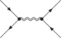
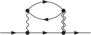
Figure 2: The diagrams which provide the order $1/(N-1)$ contributions with some higher order corrections [see Eq. (9)].

 

   

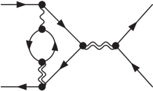
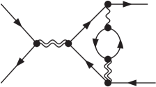
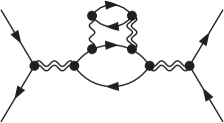
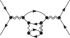
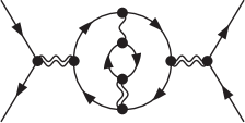
Figure 3: The order $1/(N-1)^{2}$ diagrams for the vertex function $\Gamma_{mm^{\prime};m^{\prime}m}(0,0;0,0)$ for $m\neq m^{\prime}$.

 

   

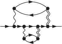
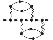
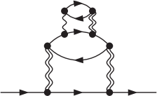
Figure 4: The order $1/(N-1)^{2}$ self-energy diagrams which contribute to the renormalization factor $z$ ($=1/\widetilde{\gamma}$).

To calculate the renormalized coupling constant $\widetilde{g}$ to order $1/(N-1)$, we need $\Gamma_{mm^{\prime};m^{\prime}m}(0,0;0,0)$ to order $1/(N-1)^{2}$ as $\widetilde{g}$ has a scaling factor $N-1$ defined in Eq. (5). The order $1/(N-1)^{2}$ contributions to the vertex function arise from the diagrams shown in Fig. 3, and from the order $1/(N-1)^{2}$ component of the vertex diagram in Fig. 2. Summing up all these contributions, $\widetilde{g}$ can be expressed in the form that is exact up to terms of order $1/(N-1)$,

$$\widetilde{g}= \ \frac{g}{1+g}\frac{1+\frac{g}{N-1}\left[1+\left(2-\frac{g}{1+g}\right)\mathcal{I}_{\phi}(g)\right]}{1+\frac{g}{N-1}\left[\frac{g}{1+g}+\mathcal{I}_{\phi}(g)\right]}+O\!\left(\!\frac{1}{N^{\prime 2}}\!\right).$$ (11)

Here, $\mathcal{I}_{\phi}(g)\equiv\pi\Delta\int\!\frac{d\omega}{2\pi}\left\{G_{0}(i\omega)\right\}^{2}\Pi(i\omega)$, and $\,N^{\prime}\equiv N-1$. This formula shows the correct asymptotic form in both the weak and the strong coupling limits: $\widetilde{g}\simeq g$ for $g\to 0$, and $\widetilde{g}\to 1$ for $g\to\infty$. Thus, Eq. (11) can also be regarded as an interpolation formula for the Wilson ratio as $R-1=\widetilde{g}/(N-1)$ at half-filling. The order $1/(N-1)$ results for $\widetilde{g}$ show an excellent agreement with the NRG results for $N=4$ as indicated in Fig. 5 (a).

To obtain Eq. (11), the parameter $\widetilde{\gamma}$ in the denominator has been taken into account up to order $1/(N-1)$,

$$\widetilde{\gamma}= \ 1+\frac{g}{N-1}\left[\frac{g}{1+g}+\mathcal{I}_{\phi}(g)\right]+\widetilde{\gamma}^{(\frac{1}{N^{\prime 2}})}+O\!\left(\!\frac{1}{N^{\prime 3}}\!\right).$$ (12)

We also calculate, $\widetilde{\gamma}^{(\frac{1}{N^{\prime 2}})}$, the order $1/(N-1)^{2}$ contributions which arise from the diagrams shown in Fig. 4 and from the higher order component of the self-energy diagram in Fig. 2.

Figure 5 (a) shows a comparison between the NRG Sakano ; Nishikawa1 and the $1/(N-1)$ expansion results for $N=4$. We see the very close agreement, especially for $\widetilde{g}$. Although the order $1/(N-1)$ results are slightly smaller than the NRG results, the two curves for $\widetilde{g}$ almost overlap each other over the whole range of $g$. The deviation must decrease as $N$ increases. Therefore, the order $1/(N-1)$ formula for $\widetilde{g}$ given in Eq. (11) provides almost exact numerical values for $N>4$. We also see in Fig. 5 (b) the value that $\widetilde{g}$ can take is bounded in a very narrow region between the curve for $N=4$ and that for the $N\to\infty$ limit. As $N$ increases, $\widetilde{g}$ varies rapidly towards the value for the large $N$ limit. The order $1/(N-1)^{2}$ results for the renormalization factor $z$, shown in Fig. 5 (a), also agree with the NRG results for $N=4$ at $g\lesssim 3.0$, or equivalently $\widetilde{g}\lesssim 0.8$, from the weak to the intermediate coupling region where $\widetilde{g}$ is still not converged to $1.0$, the value for the strong coupling limit. Therefore, away from the strong coupling regime the Kondo energy scale, $\widetilde{\Delta}=z\Delta$, can be deduced reasonably from the order $1/(N-1)^{2}$ results.

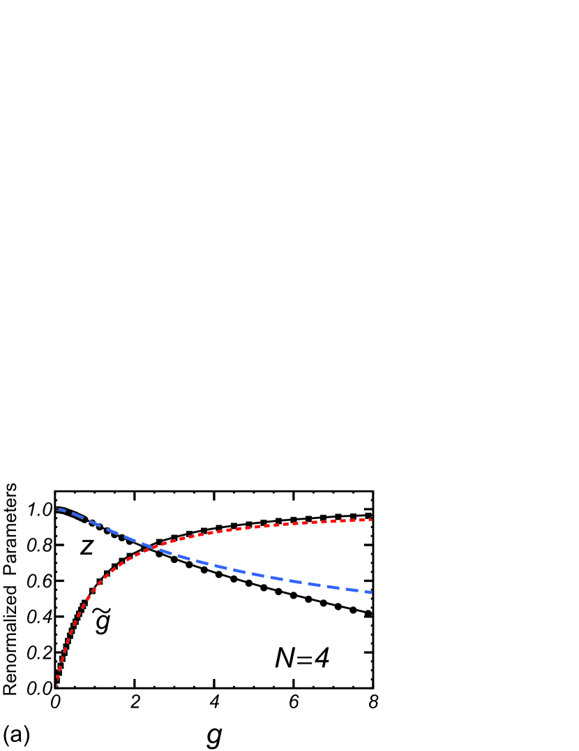
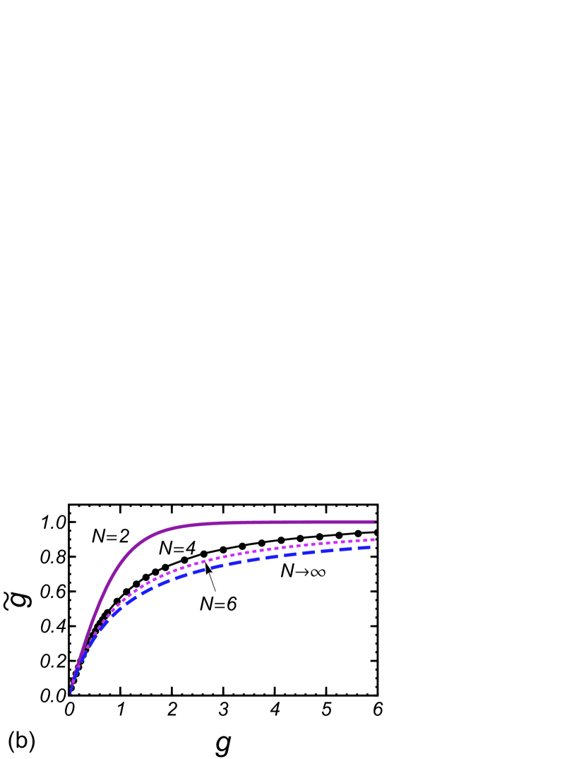
Figure 5: (Color online) (a): $\widetilde{g}$ and $z$ versus $g$ for $N=4$. The curve with the circles represents the NRG results. The red dotted line represents the order $1/(N-1)$ results for $\widetilde{g}$, and the blue dashed line the order $1/(N-1)^{2}$ results for $z$. (b): $\,\widetilde{g}\,$ vs $g$ for $N=2$ (Bethe ansats ZlaticHorvatic ), $N=4$ (NRG), $N=6$ (order $1/(N-1)$), and for $N\to\infty$ where $\widetilde{g}\to g/(1+g)$.

The $1/(N-1)$ expansion can be applied fruitfully to nonequilibrium transport at finite $U$. To be specific, we choose the lead-dot couplings and chemical potentials to be symmetric: $\Gamma_{L}=\Gamma_{R}$ and $\mu_{L}=-\mu_{R}$ ($=eV/2$). In this case, an exact expression can be derived for the retarded Green’s function at low energies up to order $\omega^{2}$, $T^{2}$, and $(eV)^{2}$ ao2001 ; Sakano ,

$$G^{r}(\omega)\simeq\frac{z}{\omega+i\widetilde{\Delta}+i\frac{{\widetilde{g}}^{2}}{2(N-1)\widetilde{\Delta}}\left[\omega^{2}+\frac{3}{4}(eV)^{2}+(\pi T)^{2}\right]}.$$ (13)

The differential conductance for the current through the impurity can be deduced from $G^{r}(\omega)$, using the formula by Meir-Wingreen MW and Hershfield HDW ,

$$\frac{dJ}{dV}=\frac{Ne^{2}}{h}\left[1-c_{T}\left(\frac{\pi T}{\widetilde{\Delta}}\right)^{2}-c_{V}\left(\frac{eV}{\widetilde{\Delta}}\right)^{2}+\cdots\right],$$ (14)

$$c_{T}=\frac{1}{3}\left(1+\frac{2\,{\widetilde{g}}^{2}}{N-1}\right),\quad\ c_{V}=\frac{1}{4}\left(1+\frac{5\,{\widetilde{g}}^{2}}{N-1}\right).$$ (15)

The low-energy behavior is characterized by the two parameters, $\widetilde{g}$ in the coefficients and $\widetilde{\Delta}$ the energy scale, which depend on $N$. Figure 6 (a) shows the ratio of $c_{V}$ to $c_{T}$ as a function of $g$ for several $N$, using Eq. (11) for $N\geq 6$. The ratio takes a value in the range ${3}/{4}\leq c_{V}/c_{T}\leq(3/4)(N+4)/(N+1)$ FootNote3 . The order $1/(N-1)$ results for $\widetilde{g}$ are numerically almost exact for $N>4$ as mentioned, and thus the results shown in Fig. 6 capture orbital effects correctly.

As another application of Eq. (11), we also consider the shot noise $S=\int\!dt\,\langle\delta\hat{J}(t)\delta\hat{J}(0)+\delta\hat{J}(0)\delta\hat{J}(t)\rangle$, where $\delta\hat{J}(t)\equiv\hat{J}(t)-\langle J\rangle$ is the current operator. At $T=0$, $S$ has been calculated to order $(eV)^{3}$ for the symmetric Anderson model for $N=2$ Sela2009 ; Fujii2010 , and for general $N$: $S=\frac{Ne^{2}}{h}\frac{1}{6}\bigl{(}1+\frac{9{\widetilde{g}}^{2}}{N-1}\bigr{)}\bigl{(}\frac{eV}{\widetilde{\Delta}}\bigr{)}^{2}eV$ Sakano . The Fano factor $F_{b}$ is defined as the ratio of $S$ to the backscattering current $J_{b}=NeV/h-J$, and has been obtained in the form Sakano ,

$$F_{b}\equiv\frac{S}{2eJ_{b}}\ =\ \frac{1+\frac{9\,{\widetilde{g}}^{2}}{N-1}}{1+\frac{5\,{\widetilde{g}}^{2}}{N-1}}\;.$$ (16)

It takes a value in the range $1\leq F_{b}\leq(N+8)/(N+4)$. In Fig. 6 (b), the order $1/(N-1)$ results for $F_{b}$ are plotted as functions of $g$ for $N\geq 6$, together with the exact results for $N\leq 4$ Sakano . As $N$ increases, $\widetilde{g}$ converges rapidly to the value, $\widetilde{g}\simeq g/(1+g)$, for the large $N$ limit, as mentioned in the above. Thus, for $N\gtrsim 8$, the $N$ dependence is determined essentially by the factor $1/(N-1)$, seen explicitly in Eq. (16). The $1/(N-1)$ expansion can also be applied to the full counting statistics SakanoFCS .

In conclusion, we have described the $1/(N-1)$ expansion approach based on the scaling defined in Eq. (5). The next leading order results for $\widetilde{g}$, which at half-filling corresponds to $\widetilde{g}=(N-1)(R-1)$, can be expressed in the form of Eq. (11). We find that this formula interpolates almost exactly between the weak and the strong coupling limits for $N\geq 4$. The $1/(N-1)$ expansion can be extended to explore the particle-hole asymmetric case FootNote1 . Furthermore, it provides a well-defined and controlled way to take into account the fluctuations near the $N\to\infty$ fixed point of many fermion systems with two-body interactions.

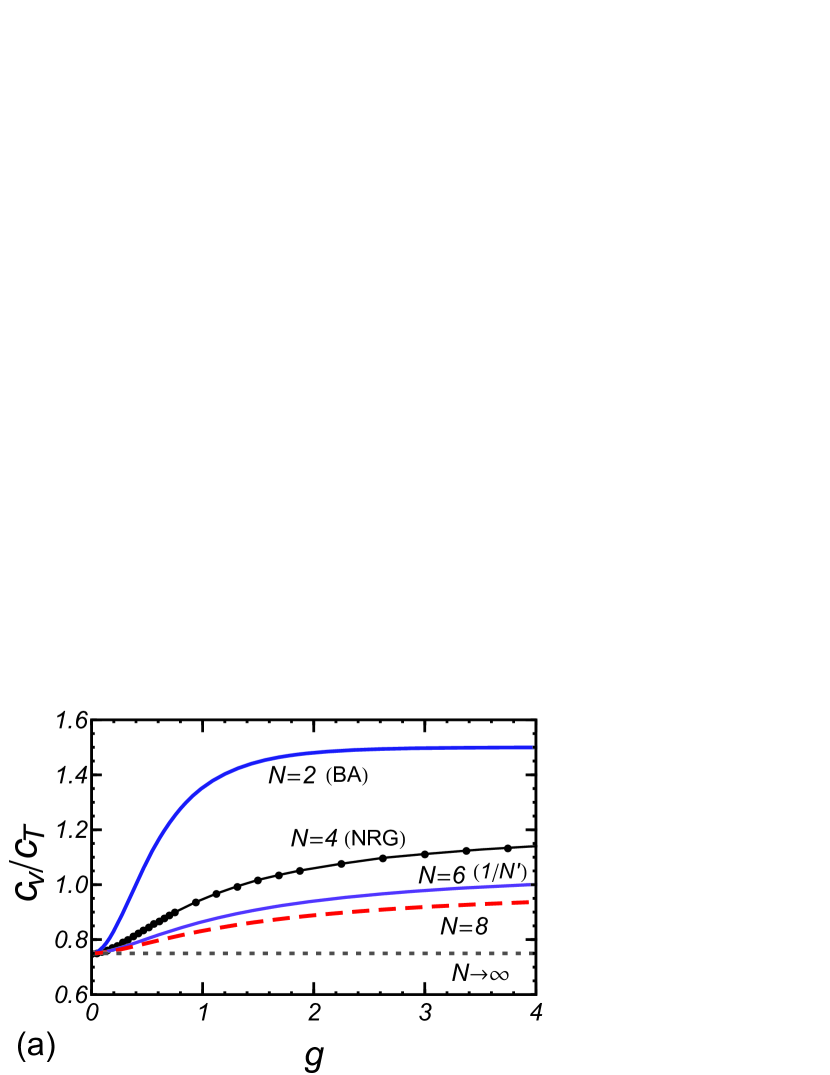
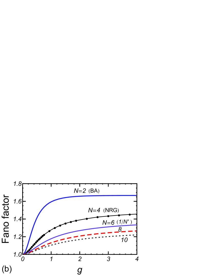
Figure 6: (Color online) Plots of (a) $c_{V}/c_{T}$ and (b) $F_{b}\,$ as a function of $g$ for $N=2$ (Bethe ansats), $N=4$ (NRG), and for $N\geq 6$ the order $1/(N-1)$ results. In the $N\to\infty$ limit, the curves approach to (a) $c_{V}/c_{T}\to 3/4$ and (b) $F_{b}\to 1$.

The authors thank J. E. Han, A. C. Hewson, and S. Tarucha for discussions. This work is supported by the JSPS Grant-in-Aid for Scientific Research C (No. 23540375) and S (No. 19104007). Numerical computation was partly carried out at Yukawa Institute Computer Facility.

References

(1)
A. C. Hewson,
The Kondo Problem to Heavy Fermions
(Cambridge University Press, Cambridge, 1993).
(2)
P. Nozières, J. Low Temp. Phys. 17, 31 (1974).
(3)
K. Yamada,
Prog. Theor. Phys. 53, 970 (1975).
(4)
V. Zlatić and B. Horvatić,
Phys. Rev. B 28, 6904 (1983).
(5)
A. Yoshimori, Prog. Theor. Phys. 55, 67 (1976).
(6)
M. Grobis,
I. G. Rau, R. M. Potok, H. Shtrikman,
and D. Goldhaber-Gordon,
Phys. Rev. Lett. 100, 246601 (2008).
(7)
G. D. Scott,
Z. K. Keane, J. W. Ciszek, J. M. Tour, and D. Natelson,
Phys. Rev. B 79, 165413 (2009).
(8)
A. Kaminski, Yu. V. Nazarov, and L. I. Glazman,
Phys. Rev. B 62, 8154 (2000).
(9)
A. Oguri, Phys. Rev. B 64, 153305 (2001).
(10)
T. Fujii and K. Ueda, Phys. Rev. B 68, 155310 (2003).
(11)
A. C. Hewson, J. Bauer, and A. Oguri,
J. Phys.: Condes. Matter. 17, 5413 (2005).
(12)
T. Delattre et al.,
Nature Phys. 5, 208 (2009).
(13)
A. O. Gogolin and A. Komnik,
Phys. Rev. B 73, 195301 (2006).
(14)
A. Golub, Phys. Rev. B 73, 233310 (2006).
(15)
C. Mora, P. Vitushinsky, X. Leyronas, A. A. Clerk, and
K. Le Hur, Phys. Rev. B 80, 155322 (2009).
(16)
E. Sela and J. Malecki,
Phys. Rev. B 80, 233103 (2009).
(17)
T. Fujii, J. Phys. Soc. Jpn. 79, 044714 (2010).
(18)
R. Sakano, T. Fujii, and A. Oguri,
Phys. Rev. B 83, 075440 (2011).
(19)
Y. Nishikawa, D. J. G. Crow, and A. C. Hewson,
Phys. Rev. B 82, 115123 (2010).
(20)
K. G. Wilson and J. Kogut,
Phys. Rep. C 12, 75 (1974).
(21)
N. Bickers, Rev. Mod. Phys. 59, 845 (1987).
(22)
K. Haule, S. Kirchner, J. Kroha, and P. Wölfle
Phys. Rev. B 64, 155111 (2001).
(23)
J. Otsuki, and Y. Kuramoto
J. Phys. Soc. Jpn. 75, 064707 (2006).
(24)
A. Georges, G. Kotliar, W. Krauth, and M. J. Rozenberg,
Rev. Mod. Phys. 68, 13 (1996).
(25)
The Hartree type self-energy is included into
.
Thus, we find
in the large limit away from half-filling.
(26)
Y. Meir and N. S. Wingreen,
Phys. Rev. Lett. 68, 2512 (1992).
(27)
S. Hershfield, J. H. Davies, and J. W. Wilkins,
Phys. Rev. B 46, 7046 (1992).
(28)
In our definition,
the experimental value by Grobis et alGrobis should be rescaled by a factor as ,
and that of Scott et alScottNatelson
as .
(29)
R. Sakano, A. Oguri, T. Kato and S. Tarucha,
Phys. Rev. B 83, 241301 (2011).