Molecular hydrogen in graphite: A path-integral simulation

Abstract

Molecular hydrogen in the bulk of graphite has been studied by path-integral molecular dynamics simulations. Finite-temperature properties of H₂ molecules adsorbed between graphite layers were analyzed in the temperature range from 300 to 900 K. The interatomic interactions were modeled by a tight-binding potential fitted to density-functional calculations. In the lowest-energy position, an H₂ molecule is found to be disposed parallel to the sheets plane. At finite temperatures, the molecule explores other orientations, but its rotation is partially hindered by the adjacent graphite layers. Vibrational frequencies were obtained from a linear-response approach, based on correlations of atom displacements. For the stretching vibration of the molecule, we find at 300 K a frequency $\omega_{s}$ = 3916 cm^-1, more than 100 cm^-1 lower than the frequency corresponding to an isolated H₂ molecule. Isotope effects have been studied by considering also deuterium and tritium molecules. For D₂ in graphite we obtained $\omega_{s}$ = 2816 cm^-1, i.e., an isotopic ratio $\omega_{s}$(H)/$\omega_{s}$(D) = 1.39.

I Introduction

In the last few years there has been a surge of interest on carbon-based materials, specially on those composed of C atoms displaying $sp^{2}$ hybridization. This group of materials includes carbon nanotubes and fullerenes, discovered in last decades, as well as graphene, found in recent years,Katsnelson (2007); Geim and Novoselov (2007) and the well-known graphite. These materials, apart from its interest in basic science, are promising tools for diverse technological applications. Thus, carbon-based systems, in general, are considered as possible candidates for hydrogen storage.Kowalczyk et al. (2005); Dillon and Heben (2001) Also, chemisorption on two-dimensional systems, such as graphene or graphite surfaces, is supposed to be important for catalytic processes.Sluiter and Kawazoe (2003)

The scientific and technological interest of hydrogen as an impurity in solids and on surfaces has existed for several decades. In principle, it seems to be one of the simplest impurities, but a clear understanding of its properties is not trivial because of its low mass, and needs the combination of advanced experimental and theoretical methods.Estreicher (1995); Pearton et al. (1992) In addition to its basic interest as an impurity, a remarkable aspect of hydrogen in solids and surfaces is its capability of passivating defects and forming complexes, facts that have been extensively studied for many years.Estreicher (1995); Pearton et al. (1992); Zeisel et al. (1999)

Experimental investigations of isolated hydrogen in graphite turn out to be difficult because of the large sensitivity required to detect this impurity, along with the presence of a large amount of hydrogen trapped at the boundaries of graphite crystallites.Atsumi (2002); Warrier et al. (2007, 2004) The stable configurations of hydrogen in the bulk of graphite have been studied in several theoretical works,Shimizu and Tachikawa (2003); Ferro et al. (2002); Diño et al. (2003) where special emphasis was laid upon both atomic and molecular forms of this impurity. Moreover, theoretical techniques have been applied to investigate the diffusion, trapping, and recombination of hydrogen on a graphite surface.Ferro et al. (2003, 2004); Sha et al. (2005); Morisset and Allouche (2008) In this respect, chemisorption of a single hydrogen atom on a graphene sheet has been studied by several authors using ab-initio methods,Sluiter and Kawazoe (2003); Duplock et al. (2004); Yazyev and Helm (2007); de Andres and Vergés (2008); Boukhvalov et al. (2008); Casolo et al. (2009) and their results show the appearance of a defect-induced magnetic moment, along with a large structural distortion.Yazyev and Helm (2007); Boukhvalov et al. (2008); Casolo et al. (2009)

For the storage of hydrogen in graphite one should also consider the presence of H₂ molecules in the graphite bulk, which are expected to be physisorbed in the interlayer space.Diño et al. (2003); Ferro et al. (2002); Atsumi (2002) Here we will focus on isolated hydrogen molecules trapped between graphite sheets. The importance of this problem is twofold: it is interesting as a point defect in materials physics, for its relevance in the stability and diffusion of hydrogen in carbon-based solids, and also H₂ in graphite is an example of a light molecule sitting and moving in a confined geometry, where quantum effects can be nontrivial.

Earlier theoretical investigations of molecular hydrogen in solids have focused on finding the lowest-energy position and stretching frequency of the molecule, including sometimes anharmonic effects obtained from the calculated potential-energy surface,Okamoto et al. (1997, 1998); Hourahine et al. (1998); Van de Walle (1998); Pruneda et al. (2002) and the quantum rotation of H₂ molecules.Fowler et al. (2002); Hourahine and Jones (2003) Density-functional electronic-structure calculations in condensed matter are nowadays very reliable, but they usually deal with atomic nuclei as classical particles, so that typical quantum effects like zero-point vibrations are not directly included. These effects can be taken into account by making use of harmonic or quasiharmonic approximations, but are difficult to consider when large anharmonicities are present, as may happen for light impurities such as hydrogen.

The quantum character of the atomic nuclei can be taken into account by using the path-integral molecular dynamics (or Monte Carlo) approach, which has been shown to be very useful in this respect. A notable benefit of this procedure is that all nuclear degrees of freedom can be quantized in an efficient and direct way, so that both quantum and thermal fluctuations are directly included in the calculations. Thus, molecular dynamics or Monte Carlo sampling applied to evaluate path integrals allows one to carry out quantitative and nonperturbative studies of anharmonic effects in many-body systems.Gillan (1988); Ceperley (1995)

In the present paper, we use the path-integral molecular dynamics (PIMD) method to study hydrogen molecules adsorbed in the interlayer region of graphite. Particular emphasis was placed upon anharmonic effects in their quantum dynamics at different temperatures. We analyze the isotopic effect on structural and vibrational properties of these molecules, by considering also molecular deuterium (D₂) and tritium (T₂). Path-integral methods similar to that employed in this work have been applied earlier to investigate hydrogen in metalsGillan (1988) and semiconductors,Ramírez and Herrero (1994); Herrero and Ramírez (1995); Miyake et al. (1998); Herrero et al. (2006); Herrero and Ramírez (2007) as well as on surfaces.Mattsson and Wahnström (1995); Herrero and Ramírez (2009a) In relation to the behavior of molecular hydrogen in confined regions, H₂ has been studied inside carbon nanotubes by diffusion Monte Carlo.Gordillo et al. (2001) Also, path-integral simulation methods have been thoroughly applied to study condensed phases of hydrogen in molecular form.Chakravarty (1999); Kaxiras and Guo (1994); Surh et al. (1997); Kitamura et al. (2000)

The paper is organized as follows. In Sec. II, we describe the computational method and the models employed in our calculations. Our results are presented in Sec. III, dealing with the spatial delocalization of H atoms, interatomic distance, vibrational frequencies, and kinetic energy. Sec. IV includes a summary of the main results.

II Computational Method

II.1 Path-integral molecular dynamics

Our calculations are based on the path-integral formulation of statistical mechanics. In this formulation, the partition function is evaluated by a discretization of the density matrix along cyclic paths, made up of a finite number $L$ (Trotter number) of “imaginary-time” steps.Feynman (1972); Kleinert (1990) In the implementation of this procedure to numerical simulations, such a discretization gives rise to the appearance of $L$ “beads” for each quantum particle. These beads can be treated in the calculations as classical particles, since the partition function of the original quantum system is isomorph to that of a classical one. This isomorphism is obtained by replacing each quantum particle by a ring polymer consisting of $L$ classical particles, connected by harmonic springs.Gillan (1988); Ceperley (1995) In many-body problems, the configuration space can be adequately sampled by molecular dynamics or Monte Carlo techniques. Here, we have used the PIMD method, which was found to require less computer time for the present problem. We have employed effective algorithms for performing PIMD simulations in the canonical $NVT$ ensemble, as those described in the literature.Martyna et al. (1996); Tuckerman (2002)

Calculations have been performed within the Born-Oppenheimer approximation, which allows us to define a $3N$-dimensional potential-energy surface for the motion of the atomic nuclei. An important issue in this type of calculations is the proper description of interatomic interactions, which should be as realistic as possible. Since effective classical potentials present many limitations to reproduce the many-body energy surface, one should resort to self-consistent quantum-mechanical methods. However, density functional (DF) or Hartree-Fock-based self-consistent potentials require computing resources that would appreciably restrict the size of our simulation cell and/or the number of simulation steps. We found a reasonable compromise by obtaining the Born-Oppenheimer surface from a tight-binding (TB) effective Hamiltonian, derived from DF calculations.Porezag et al. (1995) The capability of TB methods to simulate different properties of solids and molecules has been reviewed by Goringe et al.Goringe et al. (1997) In particular, the ability of our DF-TB potential to predict frequencies of C–H vibrations in molecular systems was shown in Refs. López-Ciudad et al., 2003; Böhm et al., 2001. We have employed earlier this TB Hamiltonian to describe hydrogen-carbon interactions in diamondHerrero et al. (2006); Herrero and Ramírez (2007) and graphene.Herrero and Ramírez (2009a) The TB energy consists of two parts; one of them is the sum of energies of occupied one-electron states, and the other corresponds to a pairwise interatomic potential.Porezag et al. (1995) Since a reliable description of the hydrogen molecule is essential for our purposes, particular attention was put on the H-H pair potential, which has been taken as in our earlier study of molecular hydrogen in silicon.Herrero and Ramírez (2009b) This pair potential reproduces the main features of known effective interatomic potentials for H₂, such as the Morse potential.Ramírez and López-Ciudad (2001)

Simulations were carried out on a graphite supercell containing 64 C atoms and one hydrogen molecule (H₂, D₂, or T₂), and periodic boundary conditions were assumed. The simulation cell includes two graphite sheets, each one being a $4\times 4$ graphene supercell of size $4a$ = 9.84 Å. An $AB$ layer stacking was considered, so that both sheets are disposed in such a way that the center of each hexagonal ring of one of them lies over a C atom of the adjacent sheet. To keep this type of stacking along a simulation run, avoiding diffusion of the graphite layers, the center-of-gravity of each layer was not allowed to move on the layer plane, which will be referred in the sequel as the $(x,y)$ plane. The average distance between sheets is a half of the supercell parameter along the $z$ axis (perpendicular to the graphite layers), and was taken to be 3.35 Å. For the reciprocal-space sampling we have used only the $\Gamma$ point (${\bf k}=0$), since the effect of employing a larger ${\bf k}$ set is a nearly constant shift in the total energy, with little influence on the energy differences between different atomic configurations. The influence of the cell size on the results of the simulations has been checked by considering graphite supercells including up to 144 C atoms (a $6\times 6$ supercell). The results found for $4\times 4$, $5\times 5$, and $6\times 6$ supercells coincided within statistical error bars. In particular, we checked the kinetic energy of the H₂ molecule (error bar of $\pm 3$ meV) and the mean H–H distance (error bar of $\pm 2\times 10^{-4}$ Å). Also, including more graphite layers in the simulation cell does not affect the results of the PIMD simulations.

Sampling of the configuration space has been carried out at temperatures between 300 and 900 K. For comparison, we also carried out PIMD simulations of pure graphite, as well as simulations of hydrogen molecules between rigid graphite sheets (in which the C atoms are kept fixed on their unrelaxed positions; see Sect. II.B for a precise definition of this approach). Moreover, some simulations were performed in the classical limit, which is obtained in our context by setting the Trotter number $L=1$. The electronic-structure calculations were performed without considering a temperature-dependent Fermi filling of the electronic states, which is reasonable for the temperature range under consideration. For a given temperature, a typical simulation run consisted of $2\times 10^{4}$ PIMD steps for system equilibration, followed by $10^{6}$ steps for the calculation of ensemble average properties. To keep roughly a constant precision in the PIMD results at different temperatures, the Trotter number was scaled with the inverse temperature ($L\propto 1/T$), so that $LT$ = 18000 K, which translates into $L$ = 60 for $T$ = 300 K. Quantum exchange effects between hydrogen nuclei were not taken into account, as they are negligible at the temperatures considered here, and both atomic nuclei in a molecule were treated as distinguishable particles.

The simulations were performed by using a staging transformation for the bead coordinates. The canonical ensemble was generated by coupling chains of four Nosé-Hoover thermostats to each degree of freedom.Tuckerman and Hughes (1998) To integrate the equations of motion, we employed a reversible reference-system propagator algorithm (RESPA), which allows one to define different time steps for the integration of fast and slow degrees of freedom.Martyna et al. (1996) The time step $\Delta t$ associated to the calculation of DF-TB forces was taken in the range between 0.1 and 0.3 fs, which was found to be appropriate for the interactions, atomic masses, and temperatures considered here. For the evolution of the fast dynamical variables, associated to the thermostats and harmonic bead interactions, we used a smaller time step $\delta t=\Delta t/4$. Note that for H₂ in graphite at 300 K, a simulation run consisting of $10^{6}$ PIMD steps needs the calculation of energy and forces with the TB code for $6\times 10^{7}$ configurations, which required the use of parallel computing.

II.2 Path centroid delocalization

We now define some spatial properties of the particle paths that will be used in the analysis of the simulation results. The center-of-gravity (centroid) of the quantum paths of a given particle is calculated as

$$\overline{\bf r}=\frac{1}{L}\sum_{i=1}^{L}{\bf r}_{i}\,,$$ (1)

${\bf r}_{i}$ being the position of bead $i$ in the associated ring polymer.

The mean-square displacement of a quantum particle along a PIMD simulation run is then given by:

$$\Delta^{2}_{r}=\frac{1}{L}\left<\sum_{i=1}^{L}({\bf r}_{i}-\left<\overline{\bf r}\right>)^{2}\right>\,,$$ (2)

where $\langle...\rangle$ indicates a thermal average at temperature $T$. After a direct transformation, one can write $\Delta^{2}_{r}$ as

$$\Delta^{2}_{r}=Q^{2}_{r}+C^{2}_{r}\,,$$ (3)

with

$$Q^{2}_{r}=\frac{1}{L}\left<\sum_{i=1}^{L}({\bf r}_{i}-\overline{\bf r})^{2}\right>\,,$$ (4)

and

$$C^{2}_{r}=\left<(\overline{\bf r}-\left<\overline{\bf r}\right>)^{2}\right>=\left<\overline{\bf r}^{2}\right>-\left<\overline{\bf r}\right>^{2}\,.$$ (5)

The first term, $Q^{2}_{r}$, is the mean-square “radius-of-gyration” of the ring polymers associated to the quantum particle under consideration, and gives the average spatial extension of the paths.Gillan (1988) The second term on the r.h.s. of Eq. (3), $C^{2}_{r}$, is the mean-square displacement of the path centroid. This term is the only one remaining in the high-temperature (classical) limit, since then each path collapses onto a single point and the radius-of-gyration vanishes. In cases where the anharmonicity is not very large, the spatial distribution of the centroid $\overline{\bf r}$ is similar to that of a classical particle moving in the same potential, and $C^{2}_{r}$ can be considered as a kind of semiclassical delocalization.

As indicated above, results of our PIMD simulations for H₂ in graphite will be compared with those obtained for rigid graphite layers. This means that in the latter case the centroids of the quantum paths corresponding to carbon atoms are kept fixed on their ideal atomic positions, so that no relaxation of the host atoms is allowed in the presence of the hydrogen molecule. This restriction allows however paths of the C atoms to be delocalized around their ideal sites, i.e. in this approach one has $C^{2}_{r}=0$ and $Q^{2}_{r}>0$ for the carbon atoms.

II.3 Anharmonic vibrational frequencies

Vibrational frequencies are often employed as fingerprints of impurities in solids, revealing information on the position that they occupy and on their interactions with the nearby hosts atoms. A traditional approach for calculating vibrational frequencies of impurities consists in obtaining the eigenvalues of the dynamical matrix associated to the atoms in the simulation cell, which yields the frequencies in a harmonic approximation. However, for light impurities the anharmonicity can be large, and the harmonic frequencies are only a first (maybe poor) approximation.

Anharmonic frequencies of vibrational modes will be calculated here by using a method based on the linear response (LR) of the system to vanishingly small forces applied on the atomic nuclei. In the context of path-integral simulations, this approach has been shown to represent a significant improvement with respect to a standard harmonic approximation.Ramírez and López-Ciudad (2001) In particular, the vibrational frequency of the H₂ stretching mode is derived by the LR method as

$$\omega_{s}=\left(\frac{k_{B}T}{\mu C^{2}_{d}}\right)^{\frac{1}{2}}\;,$$ (6)

where $k_{B}$ is Boltzmann’s constant, $\mu$ is the reduced mass of the H₂ molecule, and $C^{2}_{d}$ is the mean-square displacement of the H-H distance, $d$, that is obtained by a relation analogous to Eq. (5), after substitution of the particle coordinate $\bf{r}$ by the interatomic distance $d$. Details on this method and discussions of its capability for predicting vibrational frequencies of molecules and solids are given elsewhere.Ramírez and López-Ciudad (2001, 2002); López-Ciudad et al. (2003); Ramírez and Herrero (2005)

III Results

III.1 Atomic delocalization

For an H₂ molecule we find a minimum-energy position at an interstitial site between a carbon atom in a graphite sheet and an hexagonal ring in an adjacent sheet. At this position, the preferred orientation of the molecule is parallel to the graphite planes, in agreement with earlier calculations based on density-functional theory.Diño et al. (2003) At finite temperatures the molecule will explore other positions and orientations with respect to the graphite layers. In particular, the molecule can be tilted, forming an angle $\varphi$ with the $(x,y)$ plane.

Figure 1: Probability distribution of the angle $\varphi$ between the H–H direction and the graphite sheets, as derived from PIMD simulations at two temperatures: 300 K (solid line) and 900 K (dashed line).

In Fig. 1 we present the probability distribution of the angle $\varphi$, as derived from our PIMD simulations at two temperatures: 300 K (solid line) and 900 K (dashed line). This distribution has a maximum at $\varphi=0$ (H–H parallel to the layers), and vanishes for H–H perpendicular to the sheet plane ($\varphi=\pm 90^{o}$). As temperature increases, the probability distribution broadens slightly, but it remains as a peak centered at $\varphi=0$. However, we find that the molecule is free to rotate in the $(x,y)$ plane.

Figure 2: Probability distribution of the angle $\varphi$ between the H–H direction and the graphite sheets, as derived from PIMD simulations at 300 K. Shown are results obtained for mobile C atoms (no restrictions, solid line), as well as from a simulation in which the C atoms where kept fixed on their unrelaxed positions (fixed centroids, dashed line).

Even though there is no direct bond between molecular hydrogen and the graphite layers, the later relax slightly in the presence of the H₂ molecules, so that they follow the H₂ motion in the interlayer space. This means that the molecules are more mobile in the presence of flexible layers than in the case of stiff graphite sheets, in which the C atoms are fixed on their unrelaxed (ideal) positions. This can be visualized by looking at the distribution of the angle $\varphi$ in both cases at a given temperature. Thus, in Fig. 2 we display this probability distribution at $T$ = 300 K. The dashed line corresponds to rigid graphite sheets, whereas the solid one was obtained for flexible sheets (mobile C atoms). As expected, the distribution of the angle $\varphi$ is broader for flexible sheets, since in this case the H₂ molecule can adopt configurations that are inaccessible in the presence of rigid graphite layers. We have also calculated the same probability distribution for D₂ and T₂ for flexible sheets, and at 300 K it turns out to be similar to that shown in Fig. 2 for H₂ (solid line), but slightly narrower.

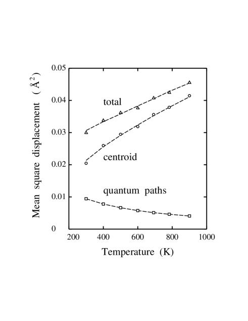
Figure 3: Spatial delocalization of atomic nuclei (protons) in H₂ along the $z$ coordinate (perpendicular to the sheet plane), as a function of temperature. Circles represent the mean-square displacement of the centroid of the quantum paths, $C_{z}^{2}$, and squares correspond to the mean-square radius-of-gyration of the paths, $Q_{z}^{2}$. The total delocalization, $\Delta_{z}^{2}$, is shown by triangles. Error bars of the total and centroid delocalization are in the order of the symbol size, whereas those of the radius-of-gyration are less than the symbol size. Dashed lines are guides to the eye.

We now turn to study the spatial delocalization of each atomic nucleus in hydrogen molecules, that is expected to include a nonnegligible quantum contribution. For our problem of H₂ in graphite, we have calculated separately both terms giving the atomic delocalization in Eq. (3), for each atom in the molecule. For a given temperature, the term $C^{2}_{r}$ does not converge to a well-defined value along a PIMD simulation, due to the onset of molecular diffusion in the interlayer space. However, its component $C_{z}^{2}$ along the $z$ axis is an equilibrium property of the molecule, as in fact it cannot diffuse across graphite layers. In Fig. 3 we display the values of $Q_{z}^{2}$ (spreading of the quantum paths, squares) and $C_{z}^{2}$ (centroid delocalization, circles), as derived from our PIMD simulations for the H₂ molecule at several temperatures. The total spatial delocalization along the $z$ coordinate, $\Delta_{z}^{2}$, is shown as triangles. In this plot, one observes that $C_{z}^{2}$ is larger than $Q_{z}^{2}$ in the whole temperature range considered. From the spatial delocalization $Q_{z}^{2}$ shown in Fig. 3, one can estimate an effective frequency for hydrogen motion in the $z$ direction. In fact, in a harmonic approximation $Q_{z}^{2}$ can be expressed analytically as a function of frequency and temperature,Gillan (1988); Ramírez and Herrero (1993) and comparing the delocalization expected for different frequencies with that given by our PIMD simulations, we found an effective frequency $\omega_{z}$ of about 1200 cm^-1.

For the spreading of the quantum paths of each H atom we obtain at room temperature $Q_{z}^{2}=9.4\times 10^{-3}$ Ų, and it decreases as temperature is raised. It is interesting to compare this value with that found for $Q_{z}^{2}$ in the case of unrelaxed graphite layers. When the C atoms are fixed on their ideal positions, we find at 300 K, $Q_{z}^{2}=5.9\times 10^{-3}$ Ų, much lower than that found when the C atoms are allowed to relax in the presence of the hydrogen molecule. It is also interesting to compare these values of the quantum delocalization in the direction perpendicular to the graphite sheets, with that on the $(x,y)$ plane. Our simulations yield $Q_{x}^{2}=Q_{y}^{2}=1.07\times 10^{-2}$ Ų and $9.9\times 10^{-3}$ Ų, for free and fixed C atoms, respectively, indicating that the quantum motion of hydrogen on the $(x,y)$ plane is only slightly affected by motion of the carbon atoms. In fact, diffusion of the H₂ molecules in the interlayer space occurs basically by classical jumps, as described elsewhere.Herrero and Ramírez (2010) However, the quantum motion in the $z$ direction is markedly affected by the relaxation of the C atoms, that contributes to enhance $Q_{z}^{2}$ by a factor of 1.6. In other words, this increase in the quantum delocalization is associated to a decrease in frequency (softening) of the vibrational modes of the H₂ molecule when full motion of the C atoms is taken into account. These modes correspond to a displacement of the whole molecule along the $z$ axis, and to the frustrated molecular rotation, with changes in the angle $\varphi$ shown in Fig. 1. We note that the quantum paths have an average extension of $\sim$ 0.1 Å at 300 K, much smaller than the H-H distance, thus justifying the neglect of quantum exchange between protons.

For the D₂ molecule we obtain at 300 K, $Q_{z}^{2}=5.4\times 10^{-3}$ Ų in the case of free motion of all atoms in the simulation cell. Comparing with the H₂ molecule, we have $Q_{z}^{2}$(H)/$Q_{z}^{2}$(D) = 1.7, clearly higher than the low-temperature limit in a harmonic approximation, given by a ratio of $\sqrt{2}$. Note that in the high-temperature limit $Q_{z}^{2}$ goes to zero, but the ratio $Q_{z}^{2}$(H)/$Q_{z}^{2}$(D) converges to the inverse mass ratio,Gillan (1988); Ramírez and Herrero (1993) in this case $m_{\rm D}/m_{\rm H}$ = 2. For T₂ we found at 300 K, $Q_{z}^{2}=3.8\times 10^{-3}$ Ų, so that $Q_{z}^{2}$(H)/$Q_{z}^{2}$(T) = 2.5, also between a ratio of $\sqrt{3}$ expected at low temperature in a harmonic approach, and the high-temperature limit given by $m_{\rm T}/m_{\rm H}$ = 3.

III.2 Interatomic distance

We first present results for classical calculations at zero temperature, where the atoms are treated as point-like particles without spatial delocalization. The interatomic potential employed here gives reliable results for molecular hydrogen in vacuo (an isolated H₂ molecule). In particular, the lowest-energy molecular configuration corresponds to a distance $R_{0}$ between hydrogen atoms of 0.741 Å. At this distance we obtain for H₂ in a harmonic approximation a stretching frequency of 4397 cm^-1.

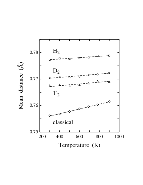
Figure 4: Mean distance between atoms in a hydrogen molecule in graphite, as derived from PIMD simulations for H₂ (squares), D₂ (circles), and T₂ (triangles). Results obtained from classical molecular dynamics simulations are also shown for comparison (diamonds). Error bars are in the order of the symbol size. Dashed lines are linear fits to the data points.

The interatomic distance between hydrogen atoms increases when the molecule is introduced from the gas phase into the graphite bulk, due to an attractive interaction between H and the nearby C atoms. For the minimum-energy distance we found in this case $R_{0}$ = 0.753 Å, which is similar to that found for the H₂ molecule in the bulk of semiconductor materials with the same interatomic potential.Herrero and Ramírez (2009b) This interatomic distance is expected to rise for increasing temperature. In fact, in a classical approximation we obtained $R$ = 0.756 Å and 0.761 Å at 300 K and 900 K, respectively. These classical results are presented in Fig. 4 as diamonds, and display a linear temperature dependence with slope $dR/dT=8.8\times 10^{-6}$ Å/K.

PIMD simulations can be also employed to study the temperature dependence of the mean interatomic distance $R$ in a quantum model. The molecular expansion with respect to the lowest-energy classical geometry is due to a combination of anharmonicity in the stretching vibration of the H₂ molecule and a centrifugal contribution caused by molecular rotation. At 300 K we find for H₂ a mean interatomic distance $R$ = 0.777 Å, to be compared with $R$ = 0.756 Å in the classical limit at the same temperature. This means that the interatomic distance of H₂ in graphite increases by 0.02 Å (about a 3%) when quantum effects are considered. For the molecules D₂ and T₂, one expects smaller interatomic distances due to their larger mass and smaller vibrational amplitudes. In fact, at 300 K we found for D₂, $R$ = 0.770 Å (i.e., $7\times 10^{-3}$ Å less than for H₂), and for T₂, $R$ = 0.767 Å. In Fig. 4 we present the temperature dependence of the mean distance for H₂ (squares), D₂ (circles), and T₂ (triangles), as derived from our PIMD simulations for full quantum motion of molecular hydrogen and host atoms. For D₂ and T₂ we find a slope $dR/dT=3.1\times 10^{-6}$ Å/K and $2.8\times 10^{-6}$ Å/K, respectively, close to the value obtained for H₂: $dR/dT=2.6\times 10^{-6}$ Å/K. Note that these changes of the interatomic distance derived from the PIMD simulations are much smaller than that found in the classical limit: $dR/dT=8.8\times 10^{-6}$ Å/K.

It is interesting to compare these changes in the mean distance $R$ with those corresponding to molecular hydrogen in the gas phase. With this purpose we carried out some PIMD simulations of an isolated hydrogen molecule with the same interatomic potential at several temperatures. These simulations yielded an increase in $R$ as temperature is raised, given by $dR/dT=7.5\times 10^{-6}$ Å/K, a value three times larger than that found for H₂ in graphite.

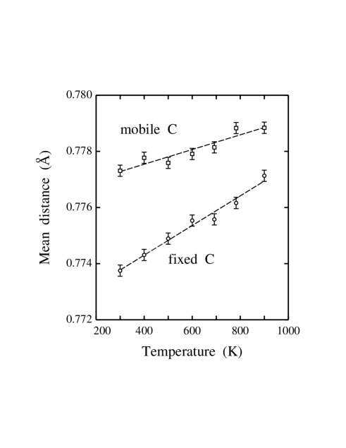
Figure 5: Mean interatomic distance for H₂ molecules in graphite, as a function of temperature. Squares indicate results derived from PIMD simulations in which all H and C atoms are mobile, whereas circles correspond to simulations in which all C atoms where kept fixed on their unrelaxed positions (fixed centroids). Dashed lines are linear fits to the data points.

It is also interesting to analyze the effect of the motion of the graphite layers on the H–H distance. We have calculated this distance in PIMD simulations in which the C atoms are kept fixed on their unrelaxed sites. The results of the interatomic distance are shown in Fig. 5 as circles. We find that the H–H distance is in this case smaller than that obtained for full quantum motion of all the atoms in the simulation cell. In fact, at 300 K the distance $R$ decreases by about $4\times 10^{-3}$ Å. However, the slope $dR/dT$ for the fixed-lattice model is larger than in the case of mobile C atoms. In fact, for fixed C atoms we find $dR/dT=5.3\times 10^{-6}$ Å/K, to be compared with a slope of $2.6\times 10^{-6}$ Å/K obtained for flexible graphite sheets.

From the zero-temperature classical calculations, we found that the H₂ molecule is expanded when it is introduced into the graphite bulk, as a consequence of the attractive C–H interaction. At finite temperatures, the H–H distance is also controlled by the centrifugal effect caused by molecule rotation. In fact, a 3D rotation is partially frustrated in the interlayer region, as shown above. In this respect, molecular rotation is favored by the relaxation of graphite sheets, thus yielding a larger centrifugal contribution to the molecule expansion than for rigid sheets.

The average interatomic distance allows us to estimate a moment of inertia for the molecule, and then the wave-number difference $\omega_{01}$ between $J=0$ and $J=1$ rotational levels. This gives for H₂, $\omega_{01}\approx 110$ cm^-1, somewhat lower than that known for the free molecule in vacuoStoicheff (1957) ($\omega_{01}=118.6$ cm^-1). For H₂ in graphite, however, the $J=1$ level will be split due to the hindered motion of the molecule for H–H perpendicular to the graphite sheets. Unfortunately, the magnitude of this splitting is not accessible from our PIMD simulations.

III.3 Stretching frequency

The stretching frequency of H₂ is an important fingerprint of the molecule, that can be used to detect and characterize this impurity in solids. We first note that the lowest-energy configuration of an isolated H₂ molecule allows us to predict a stretching frequency of 4397 cm^-1 in a harmonic approximation. From path-integral simulations combined with the LR approach presented above in Sect. II.C, we obtain for a single H₂ molecule at 300 K a frequency $\omega_{s}=4055\pm 5$ cm^-1, i.e., the anharmonic shift amounts to more than 300 cm^-1. Note that in the vibrational frequencies derived from the LR procedure, the error bars are due to the statistical uncertainty associated to the PIMD simulations.

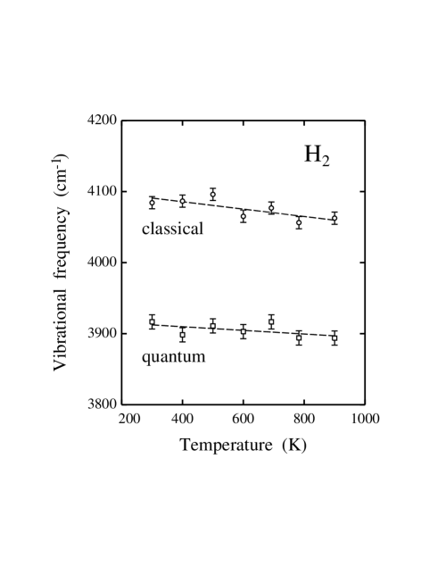
Figure 6: Frequency of the stretching vibration of the H₂ molecule in graphite as a function of temperature. Symbols represent results derived from PIMD simulations in two different approaches: squares, full quantum motion of H and C atoms; circles, classical motion of H and C atoms. Dashed lines are linear fits to the data points. Error bars correspond to the statistical uncertainty in the molecular dynamics simulations.

The stretching frequency $\omega_{s}$ is further reduced when the H₂ molecule is inserted between the graphite sheets. In fact, from our PIMD simulations at 300 K we found for H₂ a stretching frequency $\omega_{s}$ = $3916\pm 8$ cm^-1. This frequency is found to decrease slightly as the temperature is raised, as shown in Fig. 6 (squares). A linear fit to the data points gives a slope $d\omega_{s}/dT=-0.03$ cm^-1/K.

The quantum treatment of atomic nuclei in molecular dynamics simulations is decisive to give a reliable description of the vibrational frequencies of light atoms like hydrogen. In fact, we have applied the LR method to calculate the stretching frequency $\omega_{s}$ from classical simulations. At 300 K we found for H₂ in graphite a frequency $\omega_{s}=4082\pm 7$ cm^-1 (for full motion of interstitial hydrogen and host atoms), about 160 cm^-1 higher than that found in the full quantum simulations ($\omega_{s}$ = 3916 cm^-1). In Fig. 6 we have plotted the frequency $\omega_{s}$ derived from the classical molecular dynamics simulations in the temperature range from 300 to 900 K. The overestimation of vibrational frequencies in a classical approach, in comparison with the quantum results is usual in this kind of simulations,Herrero and Ramírez (2009b) since the classical calculations tend to yield results much closer to the harmonic approximation, which gives in general frequencies higher than the anharmonic ones (as is the case here).

As presented above when discussing the interatomic distance in the hydrogen molecule, there are two main factors controlling the stretching frequency of the molecule in the graphite bulk. The first one is the interaction with the graphite sheets, which tends to enlarge the H–H distance, with a concomitant decrease in the frequency $\omega_{s}$. This is the main factor contributing to the reduction observed when comparing results of an isolated molecule and a molecule in the interlayer region. The second factor is the molecular rotation, which is partially hindered between the graphite sheets, but in general causes a decrease in the vibrational frequency due to ro-vibrational coupling. All together, we find that $\omega_{s}$ decreases only slightly as $T$ is raised. This contrasts with the results obtained for the stretching frequency of H₂ in the interstitial space of silicon from PIMD simulations similar to those presented here.Herrero and Ramírez (2009b) In that case, the molecule is free to rotate in the silicon bulk, and $\omega_{s}$ is found to decrease about eight times faster than for H₂ in graphite.

For the D₂ molecule in graphite we find at 300 K a stretching frequency $\omega_{s}=2816\pm 5$ cm^-1. For increasing temperature, we obtained a trend similar to that found for H₂, with a linear decrease in $\omega_{s}$. For the isotopic shift we found a rather constant ratio between the stretching frequencies of H₂ and D₂, that amounts to 1.39, slightly smaller than the ratio expected in a harmonic approximation: $\omega_{s}$(H)/$\omega_{s}$(D) = 1.41. Experimentally, a ratio of 1.39 has been observed for the frequencies of these molecules in the gas phase.Stoicheff (1957) For comparison, we mention that in a classical simulation of D₂ at 300 K we found a stretching frequency $\omega_{s}=2896\pm 5$ cm^-1, which yields an isotopic ratio of 1.41, as in a harmonic approach. From PIMD simulations of T₂ in graphite we obtained at 300 K, $\omega_{s}=2324\pm 5$ cm^-1, so that $\omega_{s}$(H)/$\omega_{s}$(T) = 1.69, slightly lower than the harmonic expectancy of 1.73.

III.4 Kinetic energy

Path integral simulations allow one to obtain the kinetic energy $E_{k}$ of the quantum particles under consideration, which is basically related to the spread of the quantum paths. In fact, for a particle at a given temperature, the larger the mean-square radius-of-gyration of the paths, $Q_{r}^{2}$, the smaller the kinetic energy. Here we have calculated $E_{k}$ by using the so-called virial estimator, which has an associated statistical uncertainty lower than the potential energy of the system.Herman et al. (1982); Tuckerman and Hughes (1998)

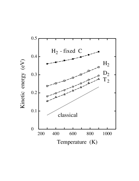
Figure 7: Temperature dependence of the kinetic energy of molecular hydrogen in graphite, as derived from PIMD simulations. Open symbols indicate results derived from simulations with full quantum motion of all atoms in the cell: squares for H₂, circles for D₂, and triangles for T₂. For comparison we also present results for H₂ with fixed C atoms (filled squares). Error bars are on the order of the symbol size. Dashed lines are guides to the eye. The dotted line corresponds to the classical limit with six degrees of freedom ($E_{k}^{\text{c}l}=3k_{B}T$).

To analyze the kinetic energy associated to the defect complex, we calculate $E_{k}$ for the simulation cell with and without the hydrogen molecule: $E_{k}$(defect) = $E_{k}$(64 C + H₂) – $E_{k}$(64 C), where we use results obtained in both series of PIMD simulations, with and without the hydrogen molecule in the graphite cell. In Fig. 7 we display the kinetic energy as a function of temperature for H₂ (squares), D₂ (circles), and T₂ (triangles). As expected, $E_{k}$ increases as temperature rises, and at a given temperature, it is larger for smaller isotopic mass. At 300 K, we find $E_{k}$ = 0.238 eV for H₂, 0.181 eV for D₂, and 0.154 eV for T₂, which gives isotopic ratios: $E_{k}$(H₂)/$E_{k}$(D₂) = 1.31 and $E_{k}$(H₂)/$E_{k}$(T₂) = 1.55. These ratios decrease as temperature is raised, and at 900 K they amount to 1.16 and 1.24, respectively, as in the high-temperature (classical) limit they should converge to unity. For comparison we also present in Fig. 7 the kinetic energy corresponding to a classical model with six degrees of freedom ($E_{k}^{\text{c}l}=3k_{B}T$, dotted line). For rising temperature, the classical kinetic energy approaches the results of PIMD simulations, in particular those corresponding to the heaviest isotope (tritium), but at 900 K it is still lower than $E_{k}$(T₂) by 43 meV (about 15% of the quantum value).

In the low-temperature limit the quotient $E_{k}$(H₂)/$E_{k}$(D₂) is expected to be close to 1.41, as obtained in a harmonic approximation. From our PIMD simulations at 300 K we obtained a ratio clearly lower than this value, what can indeed be due to the presence of anharmonicities in the molecular motion, but more importantly to the excitation of quantum levels higher than the ground state at this finite temperature. This is particularly true for molecular rotation, which is found to be rather free in the $(x,y)$ plane. Something similar can be said from the ratio $E_{k}$(H₂)/$E_{k}$(T₂) at 300 K, which is clearly lower than $\sqrt{3}$.

We have also calculated the kinetic energy of the hydrogen molecule between rigid graphite sheets. The results for $E_{k}$ obtained in this case are shown in Fig. 7 as filled squares. At 300 K we find $E_{k}$ = 0.361 eV, clearly higher than in the case of mobile carbon atoms. This decrease in kinetic energy of H₂ for flexible graphite sheets is mainly due to a softening of the vibrational modes corresponding to motion of the center-of-mass of the molecule in the interlayer space. In fact, relaxation of the C atoms in the presence of the H₂ molecule causes a decrease in the energy barriers confining the molecule at a given position, eventually favoring its motion in the graphite bulk. This decrease in $E_{k}$ is then related to the larger vibrational amplitude of the whole molecule between flexible graphite layers, indicating a nonnegligible coupling in the motion of interstitial molecule and host atoms. In connection with this, in an earlier work based on classical molecular dynamics simulations,Herrero and Ramírez (2010) it was shown that relaxation of the graphite sheets in the presence of the H₂ molecule helps to enhance molecular diffusion in the interlayer space. In particular, it was found a behavior that could not be simply explained by a single activation energy, but suggested the presence of correlations between successive molecular hops.

IV Summary

We have presented results of PIMD simulations for isolated hydrogen molecules adsorbed in the interlayer region of graphite. This kind of simulations allow us to calculate kinetic and potential energies at finite temperatures, taking into account the quantization of host-atom motions, which is not easy to consider in fixed-lattice calculations. This includes consideration of zero-point motion of guest and host atoms, which can be coupled in a non-trivial way in the many-body problem. Also, isotope effects can be readily explored, since the impurity mass appears as a parameter in the calculations.

Hydrogen molecules are found to be disposed basically parallel to the graphite-layer plane, and free to rotate in this plane. Although thermal and quantum delocalization allow the molecule to explore other orientations, molecular rotation is restricted by the nearest graphite sheets and in fact the H–H axis is not found to approach the direction perpendicular to the layers.

An important feature of H₂ molecules adsorbed in solids is their stretching vibration $\omega_{s}$. For molecular hydrogen in graphite, we find at 300 K a frequency $\omega_{s}$ = 3916 cm^-1, to be compared with $\omega_{s}$ = 4055 cm^-1 obtained for an isolated molecule with the same interatomic potential and at the same temperature. For D₂ in graphite we find a frequency of 2816 cm^-1, which gives an isotopic ratio $\omega_{s}$(H)/$\omega_{s}$(D) = 1.39, similar to those measured for free hydrogen molecules. It is remarkable that classical simulations yield for H₂ a frequency $\omega_{s}$ about 160 cm^-1 larger than the PIMD simulations. The stretching frequency of H₂ and D₂ is found to decrease slightly as temperature rises, as a consequence of coupling with molecular rotation and anharmonicities in the interatomic potential.

Results of the PIMD simulations including full quantum motion of all atoms have been compared with those obtained for rigid graphite layers. This comparison has shown that motion of carbon atoms affects appreciably several properties of the adsorbed molecules, i.e., interatomic distance, stretching frequency, kinetic energy, and atomic delocalization.

A challenging question, that should be taken into account in future work, refers to considering coupling between nuclear spins in the hydrogen molecule, i.e. dealing separately with ortho and para-H₂. This is particularly important at low temperatures, where the quantum nature of molecular rotation has to be explicitly considered in the simulations. A quantum treatment of the full problem is not trivial, being mainly complicated by the ro-vibrational coupling. Apart from equilibrium PIMD simulations such as those presented here, one can apply similar methods to study quantum diffusion of H₂ in graphite, by calculating free-energy barriers as in the case of atomic hydrogen in metalsMattsson and Wahnström (1995) and semiconductors.Herrero (1997); Herrero and Ramírez (2007)