Luminosity and mass functions of the three main sequences of the globular cluster NGC 2808

High-precision HST photometry has revealed that the globular cluster (GC) NGC 2808 hosts a triple main sequence (MS) corresponding to three stellar populations with different helium abundances. We carried out photometry on ACS/WFC HST images of NGC 2808 with the main purpose of measuring the luminosity function (LF) of stars in the three different MSs, and the binary fraction in the cluster. We used isochrones to transform the observed LFs into mass functions (MFs).

In NGC 2808 we estimate that the fraction of binary systems is $f_{\rm bin}\simeq 0.05$, and find that the three MSs have very similar LFs. The slopes of the corresponding MFs are $\alpha=-1.2\pm 0.3$ for the red MS, $\alpha=-0.9\pm 0.3$ for the middle MS, and $\alpha=-0.9\pm 0.4$ for the blue one, the same, to within the errors. There is marginal evidence of a MF flattening for masses ${\mathcal{M}}\leq 0.6{\mathcal{M}}_{\rm\odot}$ for the the reddest (primordial) MS. These results represent the first direct measurement of the present-day MF and LF in distinct stellar populations of a GC, and provide constraints on models of the formation and evolution of multiple generations of stars in these objects.

1 Introduction

The recent discoveries of multiple populations in globular clusters (GCs) have demonstrated that these stellar systems are not as simple as we first imagined. The findings of multiple evolutionary sequences in the colour magnitude diagram (CMD) of several GCs has been interpreted as sound evidence of sub-populations characterised by different ages and/or chemical abundances (Piotto et al. 2005, 2007; Milone et al. 2008; Cassisi et al. 2008; Marino et al. 2009 and references therein), and has demonstrated that these systems are not single stellar populations. In this context, helium has been proposed as a key element to interpret both the horizontal-branch (HB) morphology and the multiple and spread main sequence (MS) observed in some GCs.

The strongest indication of He-rich stellar populations in GCs is that found for NGC 2808. While spectroscopy of its red giants has long shown it to have nearly uniform iron content (Carretta et al. 2006), its main sequence is divided into three distinct sequences (D’Antona et al. 2005, Piotto et al. 2007), which have been interpreted as successive episodes of star formation.

Apart from its triple MS, NGC 2808 also displays additional observational evidence of multiple stellar populations. Its HB is greatly extended blueward, and is well populated to both the blue and the red of the instability strip (see Dalessandro et al. 2011 and references therein). The distribution of stars along the HB is multimodal (Sosin et al. 1997, Bedin et al. 2000) with three significant gaps, one of these gaps being at the colour of the RR Lyrae instability strip. Even though the HB is well populated to both the blue and the red of the instability strip, very few RR Lyrae stars have been identified in NGC 2808. The other two gaps accur along the blue extension of the HB, and delimit three distinct segments.

The red-giant branch (RGB) also exhibits evidence of non-singular populations. The CMDs shown by Yong et al.  (2008) and Lee et al. (2009) revealed a large colour spread among RGB stars that cannot be attributed to photometric errors. Furthermore, an analysis of medium-high-resolution spectra of 122 RGB stars have revealed an extended Na-O anti-correlation in NGC 2808 (Carretta et al. 2006) with the presence of three distinct groups of O-normal (peak at [O/Fe]$=+0.28$, including $61\pm 7\%$ of the stars), O-poor (peak at [O/Fe]$=-0.21$, including $22\pm 4\%$ of the stars), and super-O-poor (peak at [O/Fe]$=-0.73$, including $17\pm 4\%$ of the stars) stars. Bragaglia et al. (2010a) detected evidence of sub-populations with distinct initial He contents along the RGB of NGC 2808 by using various evolutionary features such as the dependence of the mean RGB $T_{\rm eff}$ on the He abundance.

On the basis of their relative number counts, Piotto et al. (2007) attempted to associate the three MSs with both the three HB segments defined by Bedin et al. (2000), and the three different O-content groups detected by Carretta et al. (2006).

As almost all cluster stars have the same iron content (Carretta et al. 2006), a multimodal distribution of He abundances seems to be the only way to account for both the complex HB and the multiple MS (D’Antona et al. 2005, Dalessandro et al. 2011), and is consistent with the known abundance pattern of heavy elements. Following this scenario, the population associated with the red MS (rMS) has a nearly primordial helium, while stars in the middle (mMS) and blue MS (bMS) are formed from the ejecta produced by an earlier stellar generation in the complete CNO and MgAl cycle and are He-enhanced ($Y\sim 0.32$ and $Y\sim 0.38$, respectively).

The suitability of this scenario was confirmed by Bragaglia et al. (2010b) who measured the chemical abundances of one star on the rMS and one on the bMS and found that the latter shows an enhancement of N, Na, and Al and a depletion of C and Mg, as one would expect from material polluted by a first generation of massive stars.

The idea that the multiple stellar populations discovered in many GCs can be related to the HB morphology is strongly supported by the spectroscopic study of Marino et al. (2011) of the GC NGC 6121 (M4). These authors measured oxygen and sodium directly in HB stars and found that the blue HB consists of O-poor (Na-rich, likely He-rich) stars, in contrast to O-rich (Na-poor, likely He-normal) red HB stars.

A multiple MS is also present in $\omega\,$Centauri where, a few magnitudes below the MS turn off, the MS is divides into at least three sequences (Anderson 1997, Bedin et al. 2004), with the bluer branch hosting $\sim 30\%$ of the population (Bellini et al. 2009). A spectroscopic analysis based on data acquired using the FLAMES spectrograph at the VLT by Piotto et al. (2005) revealed that, in contrast to expectations from evolution models of stars with canonical abundances, the blue MS has twice the metal abundance of the dominant red branch. In this case, we also note that the only isochrones that are able to fit these combination of colors and metallicity are greatly enriched in He (up to $Y\sim 0.38$) with respect to the old dominant component.

A divided or broad MS is not unique only to $\omega\,$Centauri and NGC 2808, but is also present in at least two other GCs: 47 Tucanae (Anderson et al. 2009) and NGC 6752 (Milone et al. 2010). In these cases, the colour spread has been tentatively attributed to small variations in He ($\Delta Y\sim$ 0.02-0.03).

Considerable effort has been dedicated to interpreting these observations. It has been suggested that the bluer MSs are formed by a distinct population of stars born from the He-enriched material polluted by the ejecta of a first stellar generation. The most appealing candidates are either intermediate-age asymptotic giant branch (AGB) stars (e.g. Ventura et al. 2002, D’Antona et al. 2005) or fast rotating massive stars (Decressin et al. 2007) although both theoretical considerations (Renzini 2008) and observational evidence (see the analysis on the Li-O correlation on the turn-off stars in the GC NGC 6752 by Shen et al. 2010) seriously challenge the rotating massive star scenario.

In this work, we investigate, for the first time, the present-day luminosity functions (LFs) and mass functions (MFs) of the three stellar populations in NGC 2808. On the basis of this study, we also derive the fraction of binaries in these three sequences and measure the fraction of stars in each population.

The paper is organised as follows. In Sect. 2, we describe the data and the data reduction. The artificial star experiments and the procedure used to obtain the completeness are illustrated in Sect. 3. In Sect. 4, we derive the fiducial of the three MSs and their colour spread. The LFs and the fraction of binaries are calculated and discussed in Sect. 5, while Sect. 6 is dedicated to the MFs of the three MSs. Finally, a summary of the main results of this project and the conclusions are given in Sect. 8.

2 Data and measurements

For this work, we used Hubble Space Telescope (HST ) data. The images were collected with the Wide Field Channel on the Advanced Camera for Surveys (ACS/WFC) under programs GO-9899 and GO-10922 and are the same as those used in Piotto et al. (2007). This dataset consists of ten exposures of $\sim 350$ s in F475W and six of the same exposure time in F814W. In addition, we also used a short-exposure image of 20 s in F475W and one of 10 s in F814W.

The photometric reduction was carried out using the software presented and described in detail in Anderson et al. (2008). It consists of a package that analyses all the exposures of each cluster simultaneously to generate a catalogue of stars in the field of view. Stars are measured independently in each image by using the point-spread function (PSF) library models from Anderson & King (2006) with a spatially constant perturbation tailored to each exposure that accounts for small focus changes due to spacecraft breathing.

This routine allowed us to detect almost every star that could be detected by eye and takes advantage of the many independent dithered pointings of each scene and the knowledge of the PSF to avoid including artifacts in the list. The ACS/WFC photometry was calibrated into the Vega-mag system by following recipes in Bedin et al. (2005) and using the zero points given in Sirianni et al. (2005).

We corrected the poor charge-transfer efficiency (CTE) in the ACS/WFC data by using the procedure and the software developed by Anderson & Bedin (2010). As an example, in the left and the middle panels of Fig. 1 we compare the ${\it m}_{\rm F814W}$ versus ${\it m}_{\rm F475W}-{\it m}_{\rm F814W}$ CMD obtained from the original images with those from the images corrected for CTE.

Figure 1: CMDs of NGC 2808 without any correction (left panel), corrected for CTE (middle panel), and corrected for both CTE and differential reddening (right panel).

2.1 Differential reddening

A visual inspection of the middle panel CMD of Fig. 1 reveals that NGC 2808 has broad MSs and sub-giant branch (SGB). Some or all of the photometric spread in color could in principle be due to either differential reddening across the observed field or to spatially dependent variations in the PSF encircled energy that are unaccounted for by the PSF model (Anderson et al. 2008). In an effort to remove the latter two effects, we adopted the procedure described in Milone et al. (2011), which we briefly summarise in the following.

For simplicity, we defined the photometric reference frame shown in Fig. 2, where the abscissa is parallel to the reddening line. To do this, we first arbitrarily defined a point (O) near the MS turn-off in the CMD of panel a. We then translated the CMD such that the origin of the new reference frame corresponds to O. Finally, we rotated the CMD counterclockwise by an angle

$\theta={\rm arctan}\frac{A_{\rm F475W}}{A_{\rm F475W}-A_{\rm F814W}}$,

as shown in Fig. 2b. For clarity, in the following, we name the abscissa and the ordinate of the rotated reference frame, ${\mathcal{X}}$ and ${\mathcal{Y}}$. The two quantities $A_{\rm F475W}$ and $A_{\rm F814W}$ are the absorption coefficients in the F475W and F814W ACS bands that, according to Bedin et al. (2005), correspond to the average reddening of NGC 2808 [$E(B-V)=0.22$ Harris 1996, 2003, $A_{\rm F475W}=0.80$, $A_{\rm F814W}=0.40$].

At this point, we adopted an iterative procedure to determine a locally valid estimate of $A_{\rm F475W}$ and $A_{\rm F814W}$ that involves the following four steps:

1. We used the rMS stars to generate the red fiducial line shown in Fig. 2b. We divided the sample of these reference stars into bins of 0.2 mag in ${\mathcal{Y}}$. For each bin, we calculated the median ${\mathcal{X}}$ that had been associated with the median ${\mathcal{Y}}$ of the stars in the bin. The fiducial was then derived by fitting these median points with a cubic spline. Here, it is important to emphasise that the use of the median allows us to minimise the influence of the outliers such as contamination by bMS, any mMS stars left in the sample, binary stars, or stars with poor photometry.

2. For each star, we calculated the distance from the fiducial line along the reddening direction ($\Delta{\mathcal{X}}$). In the right panel of Fig. 2, we plot ${\mathcal{Y}}$ versus $\Delta{\mathcal{X}}$.

3. We selected the sample of stars located in the regions of the CMD where the reddening and the fiducial line define a wide angle such that the shift in colour and magnitude due to differential reddening can be more easily separated from the random shift due to photometric errors. These stars are used as reference stars to estimate reddening variations associated with each star in the CMD and are marked in Fig. 2 as heavy black points.

4. The basic idea of our procedure, which is applied to each star (target) individually, is that differential reddening and spatially dependent PSF errors both have the effect that the stars in a local region are all shifted by the same amount to either the blue or red and in magnitude, relative to the fiducial sequence. The adopted size of the comparison region is a compromise between two competing needs. On one hand, we wish to use the smallest possible spatial cells, so that the systematic offset between the ’abscissa’ and the fiducial ridgeline will be measured as accurately as possible for each star’s particular location. On the other hand, we wish to use as many stars as possible, to reduce the error in the determination of the correction factor.

   As a compromise, for each star we selected the nearest 60 reference stars, determined the median $\Delta{\mathcal{X}}$, and assumed this to be the reddening correction for that star. In calculating the differential reddening suffered by a reference star, we naturally excluded the star itself in the computation of the median $\Delta{\mathcal{X}}$.

After the median $\Delta{\mathcal{X}}$ had been subtracted from the ${\mathcal{X}}$ value of each star in the rotated CMD, we obtained an improved CMD, which was then used to derive a more accurate selection of the sample of rMS reference stars and derive a more precise fiducial line.

After step 4, we had a newly corrected CMD. We re-ran the procedure to verify whether the fiducial sequence needed to be slightly changed in response to the adjustments made. The procedure converged after five iterations. Finally, the corrected ${\mathcal{X}}$ and ${\mathcal{Y}}$ were converted back to $m_{\rm F475W}$ and $m_{\rm F814W}$ magnitudes.

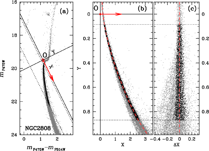
Figure 2: Panel a CMD of NGC 2808; the red arrow indicates the direction of reddening. The continuous lines are the axes (${\mathcal{X}}$ and ${\mathcal{Y}}$) of the reference frame introduced during the procedure for the measurements of reddening variations. The location of stars in this reference frame is shown in panel b, where we draw the fiducial line of the MS as a dashed red line. Reference stars are indicated with black dots and are located between the dotted lines. The rectified ${\mathcal{Y}}$ vs. $\Delta{\mathcal{X}}$ diagram is plotted in the panel c.

The result of the correction is that all the sequences of the CMD are more sharply defined. A zoom of the corrected ${\it m}_{\rm F814W}$ versus ${\it m}_{\rm F475W}-{\it m}_{\rm F814W}$ plot around the SGB and the upper-MS region is shown in the right panel of Fig. 1, where the effects of differential reddening in the original CMD are particularly evident. The whole CMD corrected for differential reddening is plotted in the left panel of Fig. 3. The Hess diagram shown in the right panel highlights the triple MS of NGC 2808, which is the main subject of the present study.

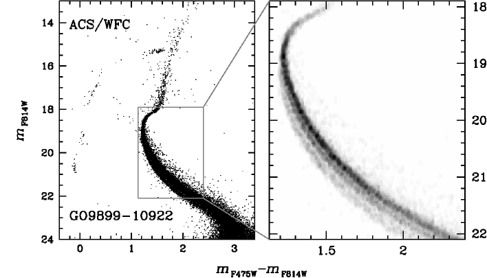
Figure 3: Left panel: CMD from ACS/WFC photometry (GO9899 and GO10922). Right panel: Hess diagram for the MS region (indicated with a grey box on the left) studied in this paper.

3 Artificial stars

The artificial-star (AS) experiments were carried out using the procedure and the software described in Anderson et al. (2008). We first produced an input list with about $5\times 10^{5}$ stars distributed across the entire WFC field of view. This list includes the coordinates of the stars in the reference frame and the magnitudes in the F475W and F814W bands. We placed artificial stars along the three MSs assuming a flat LF in the F814W band. Stellar positions were determined according to the overall cluster radial distribution by following the recipe of Milone et al. (2009).

For each object in the input list, the program described in Anderson et al. (2008) adds a star into each image with the appropriate position and flux, and measures it with the same procedure as for real stars. The AS tests are performed for one star at a time such that artificial stars never interfere with each other. We considered an AS as recovered when the input and the output position differed by less than 0.5 pixel and the input and output magnitude by less than 0.75 mag.

Artificial stars are used for several purposes: (i) to measure the completeness level of our photometry, (ii) to estimate the fraction of chance-superposition binaries, and (iii) to determine the LF of the three MSs.

3.1 Completeness

Completeness was calculated by following the procedure described in Milone et al. (2009), which accounts for both crowding conditions and stellar brightness. To account for stars of the same luminosity, but belonging to different MSs, having different colours, hence different completeness, we separately estimated the completenesses of the red, the middle, and the blue MS.

We, briefly, divided the ACS/WFC field into five annuli centred on the cluster centre and analysed AS results in seven magnitude intervals. We calculated the average completeness corresponding to each of these $5\times 7$ grid points, as the ratio of the recovered to input artificial stars within that bin, and estimated the completeness for any star at any position within the cluster by interpolating among the grid points.

The result of this procedure is illustrated in Fig. 4 for the case of the rMS. Panel a shows the completeness contours in the observational plane ${\it m}_{\rm F814W}$ versus radial distance from the centre of the cluster. The grey levels indicate the completeness of our sample with white and black colour codes corresponding to a completeness of 1 and 0, respectively. The continuous line corresponds to a completeness level of 0.50, while dotted lines indicate differences in completeness of 0.10. The observed CMD is plotted in panel b and the CMD of artificial stars in panel c. In the latter, we represented with red and black colour codes the input ASs and the observed ones, respectively. Panel d shows the completeness for rMS stars as a function of ${\it m}_{\rm F814W}$ in the five annuli into which we divided the field of view. The footprints of our data are represented in panel e, with the boundaries of each annulus marked by dotted circles.

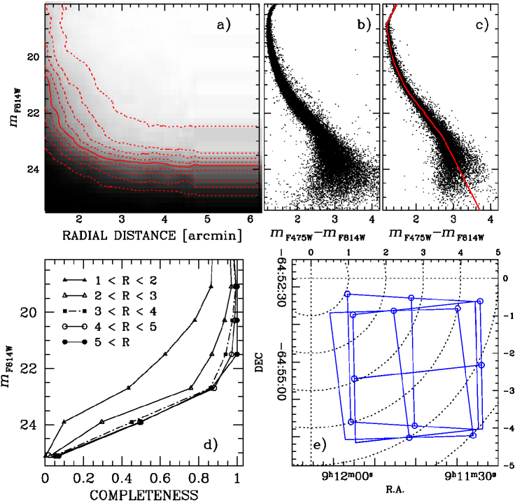
Figure 4: Panel a: Completeness contours in the ${\it m}_{\rm F814W}$ versus radial distance plane. The continuous line marks the completeness level of 0.50, while dotted lines indicate differences in completeness in steps of 0.10 units. The observed CMD and the CMD for AS (as added in red, as recovered in black) are plotted in panels b and c, respectively. Panel d shows the completeness for rMS stars as a function of ${\it m}_{\rm F814W}$ in the five annuli into which we divided the field of view. The footprints of our data are shown in panel e. [See text for details.]

4 Fiducial lines and widths of the three MSs

We now describe how we determined the fiducial lines for the three MSs and estimated their color dispersions as a function of magnitude. These results provide crucial information to help us characterise the stellar populations of NGC 2808 and are useful tools for measuring the LFs and the fraction of binaries in this GC (see Sect. 5).

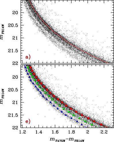
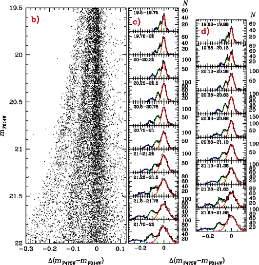
Figure 5: This figure illustrates the procedure to determine the rMS fiducial line. A region of the CMD focused on the triple MS of NGC 2808 is shown in panel a. The continuous line is the first-guess fiducial for the rMS, drawn by hand. panel b. The same CMD, after subtracting from the colour of each star the corresponding colour on the fiducial at the same magnitude. Right panels c and d show the colour distribution of stars in the 0.25 F814W magnitude intervals quoted in the inset. The continuous black lines are least squares fits of a sum of the three Gaussians that are represented as blue, green, and red lines. The $\Delta(m_{\rm F475W}-m_{\rm F814W})$ values corresponding to the peak of the red Gaussian and used to derive the red MS fiducial line are superimposed on the CMD of panel e (red filled circles). For completeness, in the latter panel we also show the fiducials for the bMS (blue triangles) and the middle MS (green squares).

Table 1: Magnitudes ($\textit{mag}=m_{\rm F814W}$), colours ($\textit{col}=m_{\rm F475W}-{\it m}_{\rm F814W}$), and colour spreads of the fiducial lines for the three MSs shown in Fig. 5.

mag	$col_{\rm rMS}$	$col_{\rm mMS}$	$col_{\rm bMS}$	$\sigma_{\rm rMS}$	$\sigma_{\rm mMS}$	$\sigma_{\rm bMS}$
19.625	1.300	1.270	1.233	0.011	0.009	0.013
19.750	1.318	1.287	1.248	0.012	0.010	0.012
19.875	1.343	1.310	1.266	0.014	0.011	0.011
20.000	1.369	1.330	1.286	0.014	0.009	0.014
20.125	1.397	1.355	1.303	0.017	0.013	0.013
20.250	1.430	1.385	1.330	0.019	0.012	0.013
20.375	1.466	1.415	1.356	0.018	0.011	0.015
20.500	1.504	1.451	1.390	0.018	0.012	0.019
20.625	1.541	1.486	1.422	0.017	0.015	0.016
20.750	1.588	1.528	1.453	0.020	0.017	0.020
20.875	1.638	1.573	1.496	0.023	0.017	0.024
21.000	1.687	1.617	1.540	0.025	0.019	0.025
21.125	1.736	1.668	1.578	0.027	0.019	0.028
21.250	1.796	1.720	1.631	0.031	0.021	0.028
21.375	1.863	1.778	1.681	0.033	0.025	0.030
21.500	1.930	1.835	1.728	0.035	0.023	0.029
21.625	2.008	1.908	1.793	0.037	0.024	0.037
21.750	2.078	1.977	1.855	0.042	0.027	0.035
21.875	2.163	2.052	1.920	0.042	0.034	0.046

The fiducial sequences and the color dispersions were determined for each MS separately using the procedure illustrated in Fig. 5, described as follows for the case of the rMS. We limited our analysis to MS stars with $19.5<{\it m}_{\rm F814W}<22$, as the three MSs can be more easily distinguished in this magnitude interval. A zoom of the ${\it m}_{\rm F814W}$ vs. ${\it m}_{\rm F475W}-{\it m}_{\rm F814W}$ CMD of Fig. 3 is shown in panel a, where the red line is a first-guess fiducial line for the rMS drawn by hand. In panel b, we subtracted from the color of each star the colour of the rMS fiducial line at the same magnitude of the star. The following two panels show the colour distribution of the stars in panel b. Specifically, in panels c we plotted the colour distribution in ten intervals of 0.25 F814W magnitudes from ${\it m}_{\rm F814W}=19.5$ to ${\it m}_{\rm F814W}=22.0$, while panel d shows the color distribution in nine $m_{\rm F814W}$ bins between 19.75 and 21.75.

As widely discussed in Piotto et al. (2007), the histogram distributions clearly show three distinct peaks, which we fitted using a least squares method with the sum of three Gaussians represented as a continuous black line. The single Gaussian components that fit each MS are plotted with blue, green, and red lines. The $\Delta(m_{\rm F475W}-m_{\rm F814W})$ values corresponding to the peak of the red Gaussian are plotted as red-filled circles in the CMD of panel e. The rMS fiducial line was obtained by fitting these red squares by means of a spline and is represented as a continuous red line.

Note that both the bMS and the mMS are not vertical in the $m_{\rm F814W}$ vs. $\Delta(m_{\rm F475W}-m_{\rm F814W})$ diagram of panel b. As a consequence of this, the dispersions of the blue and green Gaussian are not used to estimate the color spread and the fiducials of these MSs. To determine these quantities, we instead followed a procedure similar to the one just described for the rMS, but in these cases we subtracted from the observed colour of each star, the colour of the mMS (or the bMS) at the corresponding F814W magnitude. For completeness, the fiducials of the mMS (in green) and bMS (in blue) are also plotted in panel e, while the $m_{\rm F475W}-m_{\rm F814W}$ colours and the $m_{\rm F814W}$ magnitudes of the three fiducial lines are listed in Table 1.

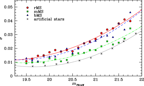
Figure 6: Observed color dispersion of the bMS (blue triangles), mMS (green squares), rMS (red circles), and AS (black crosses), as a function of the F814W magnitude. Continuous, dashed-dotted, dashed, and dotted lines are the best-fit parabolas for the rMS, mMS, bMS, and the rMS AS, respectively.

The dispersions obtained for the bMS ($\sigma_{\rm bMS}$), mMS ($\sigma_{\rm mMS}$), and rMS ($\sigma_{\rm rMS}$), and the dispersion of artificial stars ($\sigma_{\rm AS}$) are plotted in Fig. 6 as a function of $m_{\rm F814W}$. The continuous, dashed-dotted, dashed, and dotted lines are the best-fit second-order polynomials for the three MSs (${\it P}_{\rm bMS,mMS,rMS}$) and for the simulated CMD ($P_{\rm AS}$).

As expected, the MS spread for the artificial stars is slightly smaller than the colour spread of real stars. This is the consequence of an important limitation of artificial-star tests, and is widely discussed in Anderson et al. (2008) and Milone et al. (2009) for the case of ACS/WFC images. While artificial stars are measured by using the same PSFs used to generate them, for real stars we are unable to obtain a perfect PSF model. The PSF for a real star is constructed to reproduce as well as possible the profile of the real stars, but we cannot avoid having some errors in the PSF model; our real-star measurements will suffer from these errors, but our artificial-star measurements will not. We note that this additional dispersion for real stars does not allow us to exclude the effect of the intrinsic broadening of the MSs, which could be caused by an intrinsic dispersion in $Z$, $Y$, or a combination of the two (see e. g. Marino et al. 2009 and Anderson et al. 2009). In this context, we note that while the measured $\sigma_{\rm bMS}$ values do not differ significantly from $\sigma_{\rm rMS}$, the mMS does have a marginally smaller dispersion over the whole range of magnitude we analysed. It is tempting to conclude that the different colour width of the mMS could be due to a smaller intrinsic spread than those of both bMS and rMS. However, our data do not allow us to conclude that this difference is significant.

So that we can compare the observed and simulated MSs we added an additional error component into the artificial-star colors. To do this, we added to the colour of each bMS (mMS, rMS) artificial star an error randomly extracted from a Gaussian distribution with a dispersion $P_{\rm DIF}=\sqrt{P_{\rm bMS(mMS,rMS)}^{2}-P_{\rm AS}^{2}}$ (see Milone et al. 2009 for more details).

5 The luminosity function of the three MSs

We present the recipe used to determine both the fraction of binaries and the LFs of the three stellar populations of NGC 2808. Specifically, Sect. 5.1 describes the stellar models used to determine the mass-luminosity relations involved in the measurement of the binary fraction and estimate the MFs. Sect. 5.2 analyses the behaviour of binaries in the CMD of NGC 2808, while in Sect. 5.3 we describe in detail the procedure used to measure the LFs and the fraction of binaries and discuss the results.

5.1 Isochrones

To convert the LFs into MFs, we used the mass-luminosity relation from the stellar models in Dotter et al. (2007), and an independent set of models specifically computed for this project. At the low-mass end, these additional stellar models correspond to the very low-mass (VLM) range (${\mathcal{M}}<0.5{\mathcal{M}}_{\rm\odot}$) and rely on the equation of state and the boundary conditions in Cassisi et al. (2000). For more massive stars, we adopted the same physical scenario adopted by Pietrinferni et al. (2004, the BaSTI archive). Considerable care was devoted to performing an accurate match —avoiding any discontinuity that could affect the resulting mass-luminosity relation— between stellar models in the VLM regime and more massive structures. The stellar models were used to compute various sets of isochrones for a metallicity suitable for NGC 2808 and various He abundances. The whole set of models (hereafter BaSTI models) were transformed from the theoretical plane to the ACS observational one by means of theoretical color transformations and bolometric corrections for the standard Johnson bandpasses provided by Allard et al. (1997) and, then applying the equations provided by Sirianni et al. (2005) to convert the ground-based Johnson magnitudes to the HST  ACS filters.

Since spectroscopic studies have demonstrated that NGC 2808 stars have homogeneous iron contents, the only way to fit the three MSs is to assume that the rMS has a canonical He content, while the mMS and the bMS are matched by He enriched isochrones (Piotto et al. 2007). We were able to fit the rMS with an isochrone with $Y=0.248$ and the closest matches between the mMS and bMS were obtained by assuming that $Y\sim 0.31$-32 and $Y\sim 0.38$, respectively.

The comparison between the observed CMD and the isochrones is shown in the left panels of Fig. 7 for the Dotter et al. (2007) isochrones (bottom panel) and for the BaSTI models (upper panel). The values of metallicity, $Y$, distance modulus, and foreground reddening that provide the closest match are provided in the inset of Fig. 7 and are listed in Table 2.

The three stellar populations should have almost the same age but stars along the bMS and the mMS are less massive than rMS stars of the same luminosity. Right panels show the relation between ${\it m}_{\rm F814W}$ and stellar mass predicted by theoretical models for stars of the triple MS.

From Fig. 7, it appears that both sets of isochrones do not accurately reproduce the turn-off portion of the CMD. The fit could be slightly improved by adopting a different choice of cluster age, but in any case some disagreement would be still present as a consequence —probably— of some residual drawback in the available color-effective temperature relation and bolometric correction scale. Nevertheless, we wish to emphasize that this mismatch between theory and observations in the turn-off region does not affect our present investigation, since we measure the MF far below the mass where evolutionary effects are significant.

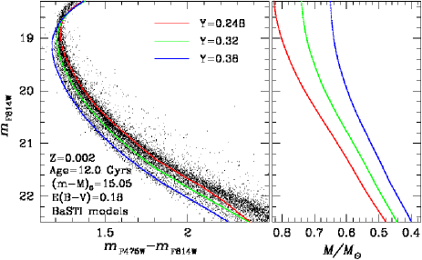
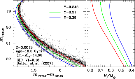
Figure 7: Left panels. Best-fit isochrones from Pietrinferni et al. (2004) (top) and Dotter et al. (2007) (bottom) superimposed on the CMD of Fig. 3. Best-fit parameters are listed in the inset. Right panels show the luminosity in the F814W band as a function of the stellar mass.

Table 2: Basic properties of NGC 2808 inferred from the isochrones used in the paper.

Model	$Z$	Age	${\rm(m-M)_{0}}$	E(B-V)	$Y$(rMS - mMS - bMS)
BaSTI	0.0020	12.0 Gyrs	15.05	0.18	0.248 - 0.32 - 0.38
Dotter et al. (2007)	0.0013	13.0 Gyrs	14.96	0.16	0.248 - 0.31 - 0.38

5.2 Photometric MS-MS binaries

At the distance of NGC 2808 ($d\sim 9.6$ Kpc, Harris 1996, update 2003), binary stars are completely unresolved, and the light from both stars combines to form a single point-like source. Specifically, if we indicate with $m_{1}$ and $m_{2}$ the magnitudes, and $F_{1}$ and $F_{2}$ the fluxes of the two components, the binary will appear as a single object with a magnitude

$m_{\rm bin}=m_{1}-2.5\leavevmode\nobreak\ \log{(1+\frac{F_{1}}{F_{2}})}$.

For a simple stellar population, the luminosity of binary systems formed by two MS stars depends on the mass ratio ($q=\mathcal{M}_{2}/\mathcal{M}_{1},\mathcal{M}_{2}<\mathcal{M}_{1}$) of the two components as stellar masses ($\mathcal{M}_{1}$, and $\mathcal{M}_{2}$) are directly related to the luminosity. The equal-mass binaries form a sequence that is parallel to the MS, but about 0.75 magnitudes brighter. When the masses of the two components are different, the binary will appear redder and brighter than the primary and populate a CMD region on the red side of the MS ridge line (MSRL) and below the equal-mass binary line. As a consequence of this, the binaries formed by stars of similar mass can be easily discerned photometrically from the single MS stars as they have large offsets from the MSRL, whereas in the CMD it is hard to distinguish binary systems formed by stars that strongly differ in mass because of their small colour offset from the MSRL.

To calculate the total fraction of binaries in NGC 2808, we follow an approach adopted by several authors (e. g. Rubenstein & Bailyn  1997, Zhao & Bailyn  2005, Sollima et al. 2007, Milone et al. 2010, 2011) that consists of simulating a binary population that follows a given distribution of mass ratios [f(q)] and in comparing the observed and simulated CMDs.

The adopted f(q) is crucial for a correct measurement of the binary fraction. To date, the only constraint on the shape of f(q) in GCs comes from the work of Milone et al. (2011), who studied the main properties of the population of MS-MS binaries in 59 Galactic GCs and found that the mass-ratio distribution is generally flat for $q>0.5$. Unfortunately, these authors were unable to place any constraints on mass ratios smaller than $q=0.5$. For simplicity, in this work, we extrapolate the flat mass-ratio distribution all the way down to $q=0$.

In Appendix A, we derive the fraction of binaries and the MFs of the three MSs by using a different mass-ratio distribution. We show that the use of a different f(q) does not change the main conclusions of this paper.

A further complication, in the case of NGC 2808, is the triple stellar population. Until now, there have been neither observational nor theoretical constraints on the origin of the components of binary systems in GCs with multiple MSs. In particular, we do not know whether the components of a binary system belong preferentially to the same stellar population or originate from different MSs.

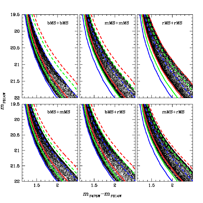
Figure 8: Upper panels: Simulated CMDs for MS-MS binaries formed by pairs of bMS (left), mMS (middle), and rMS stars (right). Bottom panels: binaries composed by bMS and mMS (left), bMS and rMS (middle), and mMS and rMS stars (right). Continuous lines are the empirical MSRLs for the three MSs while sequences of equal mass bMS, mMS, and rMS binaries are marked with dashed lines.

In the upper panels of Fig. 8, we used our empirical MSRLs and the mass-luminosity relations of Pietrinferni et al. (2004) to generate sequences of MS-MS binary systems formed by pairs of stars belonging to the same population (i. e. pairs of bMS+bMS, mMS+mMS, and rMS+rMS stars). The bottom panels show the CMDs for binaries made of stars from different MSs. (This is not inconceivable; GCs are dynamically evolving objects and binaries can be destroyed and re-created over a Hubble time.) The MSRLs of the bMS, mMS, and rMS have been represented with blue, green, and red continuous lines and we have marked with dashed lines the sequences of equal mass bMS, mMS, and rMS binaries. In all cases, we assumed a flat mass-ratio distribution.

While the determination of the frequency of each of these groups of binaries is beyond the scope of this paper, it is clear that the results of this paper may depend in some way on the different scenario we adopt. To account for this, we determine the binary fraction and the LFs by assuming two extreme scenarios. In Sect. 5.3, we describe in detail the adopted procedure considering only one of these extreme scenarios which assumes that each component of a binary system has the same probability of belonging to any MS.

In Appendix B, the other extreme scenario is considered, i. e. that both the components of all binary systems belong to the same MS. We demonstrate that the two extreme scenarios predict differences in the binary fraction that are less than 0.01, hence that the obtained MFs do not depend significantly on the adopted scenario.

5.3 Luminosity functions

We describe the iterative procedure used to derive both the LFs of the three MSs and the total binary fraction ($f^{\rm BIN}$) in NGC 2808.

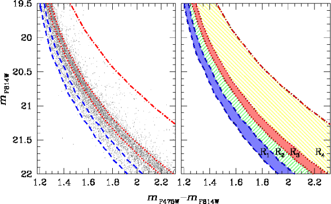
Figure 9: Left panel: ${\it m}_{\rm F814W}$ vs. ${\it m}_{\rm F475W}-{\it m}_{\rm F814W}$ CMD for MS stars. Blue dashed lines and red dotted lines are the MSRLs of the bMS and the rMS blue and red-shifted by $\pm$ three times $\sigma_{\rm bMS}$ and $\sigma_{\rm rMS}$. The red dashed-dotted line is displaced to the red from the fiducial of equal-mass rMS-rMS binaries by $+3$ times $\sigma_{\rm rMS}$. These lines are the boundaries of the shaded areas in the right panel that define the four regions used to calculate the LFs of the three MSs and the binary fraction (see text for details).

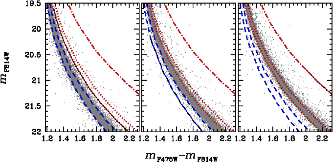
Figure 10: Simulated CMD for single bMS (left), mMS (middle), and rMS (right) stars. We superimposed on each CMD the boundaries of the four regions defined in Fig. 9.

To illustrate our setup, the left panel of Fig. 9 shows a zoom of the external field CMD around the region where the division in the MS is most evident. The two red dotted lines are constructed by adding and subtracting from the colour of the rMSRL a value equal to three times $\sigma_{\rm rMS}$. Similarly, the blue dashed lines are the bMSRL shifted to the blue and red by three times $\sigma_{\rm bMS}$. The red dot-dashed lines mark the loci of equal-mass rMS-rMS binaries red-shifted by $3\times\sigma_{\rm rMS}$. The four regions delimited by these five lines are marked in the right panel with different colour codes and are named $R_{1}$, $R_{2}$, $R_{3}$, and $R_{4}$.

The bulk of bMS stars are located within the region $R_{1}$, while regions $R_{2}$ and $R_{3}$ are mainly populated by mMS and rMS stars. Region $R_{4}$ mainly contains binary systems formed by a pair of MS stars. Obviously not all the single b(m,r)MS stars are located within $R_{1(2,3)}$ but a fraction of them migrates to nearby regions because of the measuring error. In addition, all these regions are also populated by binaries.

We use AS tests to estimate the fractions of the “misplaced” (and of the correctly placed) single stars. To each region $R_{\rm i}$, we associate a fraction $f^{\rm rMS}_{\rm i}$ of rMS stars, a fraction $f^{\rm mMS}_{\rm i}$ of mMS stars, and a fraction $f^{\rm bMS}_{\rm i}$ of bMS stars. This is illustrated in Fig. 10, where we show the simulated CMDs for single stars of bMS (left panel), mMS (middle panel), and rMS (right panel).

In an analogous way we add artificial binary systems —once assumed a binary distribution and a mass-ratio distribution— and infer the fraction of binaries $f^{\rm BIN}_{\rm i}$ that fall within each CMD region $R_{\rm i}$, as we later see.

Our observables are the total numbers $N_{\rm i=1,2,3,4}$ (corrected for completeness) of stars within each region $R_{\rm i=1,2,3,4}$, which can be expressed as the sum of four terms containing the four unknown $N_{\rm bMS}$, $N_{\rm mMS}$, $N_{\rm rMS}$, and $f^{\rm BIN}$, according to the four relations (for $i=1,2,3,4$)

$$N_{\rm i}=N_{\rm bMS}f^{\rm bMS}_{\rm i}+N_{\rm mMS}f^{\rm mMS}_{\rm i}+N_{\rm rMS}f^{\rm rMS}_{\rm i}+f^{\rm BIN}N_{\rm MS}f^{\rm BIN}_{\rm i},$$ (1)

where the symbols $N_{\rm bMS}$, $N_{\rm mMS}$, and $N_{\rm rMS}$ are the total number of single bMS, mMS, and rMS in our sample, and for convenience we have introduced the quantity $N_{\rm MS}=N_{\rm bMS}+N_{\rm mMS}+N_{\rm rMS}$, which is the total number of single stars in our sample. Finally, the quantity $f^{\rm BIN}$ expresses, as a fraction of $N_{\rm MS}$, the unknown total binary fraction.

To obtain the LFs, we need to estimate the unknowns quantities $N_{\rm bMS}$, $N_{\rm mMS}$, $N_{\rm rMS}$, and $f^{\rm BIN}$ at different magnitude intervals. As an adequate compromise, we chose to divide the CMD into intervals of 0.25 mag in $m_{\rm F814W}$, within which we estimated: $N_{\rm i=1...4}$, $f^{\rm bMS}_{\rm i=1...4}$, $f^{\rm mMS}_{\rm i=1...4}$, and $f^{\rm rMS}_{\rm i=1...4}$ for each magnitude bin.

However, there is an interplay between the $f^{\rm BIN}_{\rm i}$ and the LFs, as the $f^{\rm BIN}_{\rm i}$ depend strongly on the LFs and visa-versa. To break this degeneracy, we adopted an iterative procedure. At the first iteration, we assumed $f^{\rm BIN}=0$ and solve the system of four forms ($i=1,2,3,4$) of Eq. 1 in the unknowns $N_{\rm bMS}$, $N_{\rm mMS}$, and $N_{\rm rMS}$. These numbers provide us with the first (crude) estimates that we use to determine the $f^{\rm BIN}_{\rm i}$.

To determine $f^{\rm BIN}_{\rm i}$, we created a simulated “pure binary” CMD under the assumptions given in previous section (i. e. a flat f(q) and the binary components belonging to any of the MSs). We draw the primary member of the binary from the current observed distribution of stars for each sequence, constructing an artificial-star catalog 10$\times$$N_{\rm bMS}$ bMS stars, $10\times N_{\rm mMS}$ mMS stars, and $10\times N_{\rm rMS}$ rMS stars (the factor of ten providing us with higher quality statistics). For each of these stars, we determine, based on the F475W and F814W magnitudes and the mass-luminosity relation of Pietrinferni et al. (2004), the corresponding mass ($\mathcal{M}_{1}$) which we then associate with a secondary that has a mass randomly drawn between 0.08 $\mathcal{M}_{\odot}$ and $\mathcal{M}_{1}$. We then add the flux of the secondary to that of the primary and arrive at the magnitudes for the binary system.

The Hess diagram of the resulting CMD is shown in Fig. 11 with the boundaries between the four CMD regions superimposed. This CMD can then be used to estimate the fraction of binaries $f^{\rm BIN}_{\rm i}$ in each region $R_{\rm i}$, by computing the ratio of the number of binaries within each region, and the total inserted binaries.

With the values of $f^{\rm bMS}_{\rm i}$, $f^{\rm mMS}_{\rm i}$, $f^{\rm rMS}_{\rm i}$ and a first guess of the values of $f^{\rm BIN}_{\rm i}$ we can now solve the system of four equations (Eq. 1) in the four unknown $N_{\rm bMS}$, $N_{\rm mMS}$, $N_{\rm rMS}$, and $f^{\rm BIN}$. This ends one iteration.

With the improved estimates of $N_{\rm bMS}$, $N_{\rm mMS}$, $N_{\rm rMS}$, we simulated a new CMD, improved our estimates of $f^{\rm BIN}_{\rm i}$, and again solved Eq. 1 for $N_{\rm bMS}$, $N_{\rm mMS}$, $N_{\rm rMS}$, and $f^{\rm BIN}$. We iteratively repeated the procedure until convergence is reached, i. e. until the $f^{\rm BIN}$ value changed by less than 0.001 from one iteration to the successive one.

The procedure converges to a total binary fraction for NGC 2808 of $f^{\rm BIN}=0.045\pm 0.011$, and to the three LFs for the three individuals MSs displayed in Fig. 12. Star counts for bMS, mMS, and rMS for each magnitude bin are listed in Table 3. The associated errors are Poisson errors and represent a lower limit to the true uncertainties in the star counts and the binary fraction. An inspection of this figure suggests that the three LFs have a similar trend with magnitude; they increase up to ${\it m}_{\rm F814W}\sim 20.5$ and then remain nearly constant at fainter magnitudes. Figure 13 directly compares the observed CMD (on the left) and the simulated CMD (in the middle) during the last iteration. The right panel shows the difference between these two.

The sum over all the magnitude bins of the quantities $N_{\rm bMS}$, $N_{\rm mMS}$, and $N_{\rm rMS}$ provides a measure of the population ratios among the MSs. The fraction of stars in one of the MSs with respect to the total number of single MS stars ($N_{\rm MS}$) are: ($N_{\rm rMS}/N_{\rm MS}$; $N_{\rm mMS}/N_{\rm MS}$; $N_{\rm bMS}/N_{\rm MS}$)$=$ ($62\pm 2$; $24\pm 2$; $14\pm 3$)%.

We note that these numbers are different from the crude estimate given in Table 1 of Piotto et al. (2007), and much in closer agreement with the fraction of (O-normal; O-poor; Super-O-poor) $=$ ($61\pm 7$; $22\pm 4$; $17\pm 4$)% based on the RGB stars sample presented in Carretta et al. (2006).

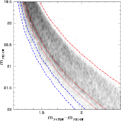
Figure 11: Hess diagram of a simulated CMD for MS-MS binaries alone. We used a flat mass-ratio distribution and considered that the two components of a binary system have the same probability of belonging to any given MS. We superimposed on each CMD the boundaries of the four regions defined in Fig. 9.

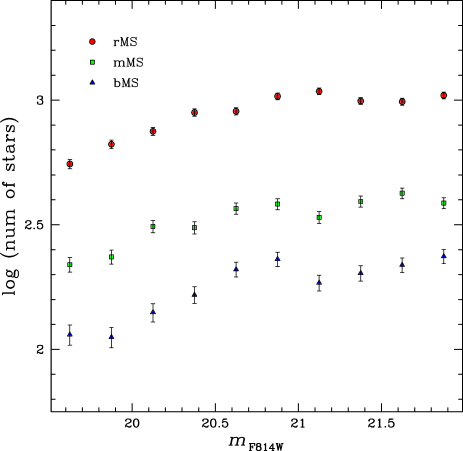
Figure 12: Luminosity function for the three MSs.

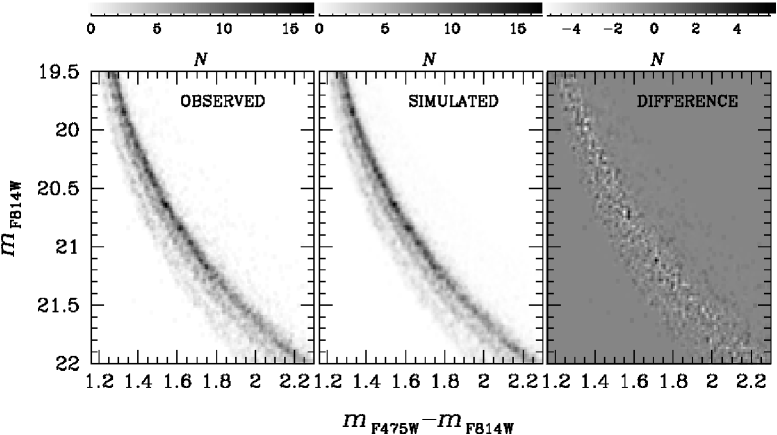
Figure 13: Hess diagram of the observed CMD (left), the simulated CMD (middle), and difference between the observed and simulated Hess diagrams (right).

Table 3: Numbers of rMS, mMS, and bMS stars, corrected for completeness, per magnitude and mass interval.

$\Delta{\it m}_{\rm F814W}$		$\Delta{\mathcal{M}}$			Number of stars
	rMS	mMS	bMS	rMS	mMS	bMS
19.50-19.75	0.751-0.770	0.684-0.699	0.611-0.623	$485\pm 22$	$204\pm 14$	$103\pm 10$
19.75-20.00	0.729-0.751	0.667-0.684	0.597-0.611	$595\pm 24$	$213\pm 15$	$102\pm 10$
20.00-20.25	0.705-0.729	0.646-0.667	0.581-0.597	$671\pm 26$	$294\pm 17$	$126\pm 11$
20.25-20.50	0.680-0.705	0.624-0.646	0.564-0.581	$826\pm 29$	$294\pm 17$	$156\pm 12$
20.50-20.75	0.654-0.680	0.602-0.624	0.544-0.564	$836\pm 29$	$353\pm 19$	$196\pm 14$
20.75-21.00	0.628-0.654	0.578-0.602	0.524-0.544	$958\pm 31$	$363\pm 19$	$220\pm 15$
21.00-21.25	0.603-0.628	0.556-0.578	0.504-0.524	$1008\pm 32$	$323\pm 18$	$172\pm 13$
21.25-21.50	0.579-0.603	0.534-0.556	0.484-0.504	$922\pm 30$	$376\pm 19$	$192\pm 14$
21.50-21.75	0.555-0.579	0.512-0.534	0.465-0.484	$924\pm 30$	$409\pm 20$	$206\pm 14$
21.75-22.00	0.530-0.555	0.489-0.512	0.442-0.465	$967\pm 31$	$369\pm 19$	$224\pm 15$

6 The mass functions of the three MSs

The LFs can be transformed into MFs by using a theoretical mass-luminosity relation. However, we note that there is some uncertainty in this approach, mainly related to the still significant uncertainties that affect the color-$T_{\rm eff}$ relations and bolometric correction scales needed to transform the model predictions from the theoretical plane to the observational one (see the discussion in Cassisi 2007).

The models we used in this paper account for the different helium content of the three MSs and allow us to gather information on the shape of the MFs of the three MSs of NGC 2808. In Fig. 14, we compare the MFs derived from the LFs of Fig. 12 by using the mass-luminosity relation of Pietrinferni et al. (2004) and Dotter et al. (2007). We note that the error bars represent the Poisson errors only (derived from the Poisson error of the star counts in the LF), hence must be considered a lower limit to the true MF errors. The magnitude intervals have been transformed into mass intervals using the BaSTI mass-luminosity relations and are listed in Table 3. We fitted the resulting values by applying a least squares fit of straight lines. Best-fit lines are plotted as black continuous lines, while gray dotted-dashed lines represent the minimum- and maximum-slope lines.

If we assume that the MF is described by a power law of the form ${\it dN}/d{\mathcal{M}}\propto{\mathcal{M}}^{\rm\alpha}$, we have for the bMS, the mMS, and the rMS the slopes ($\alpha$) of $-1.20\pm 0.20$, $-0.84\pm 0.22$, and $-0.84\pm 0.28$, respectively in the case of a Pietrinferni et al. (2004) mass-luminosity relation, while the Dotter et al. (2007) models give for the three MSs slightly steeper MFs with slope of $-1.29\pm 0.17$, $-1.01\pm 0.21$, and $-0.88\pm 0.32$. These numbers indicate that there is no evidence of a significant difference among the slopes of the three MSs, in the limited mass interval considered in the present study. However, we note that the MF for the rMS does appear to flatten below ${\mathcal{M}}/{\mathcal{M}}_{\rm\odot}\sim 0.6$, at variance with the other two MFs.

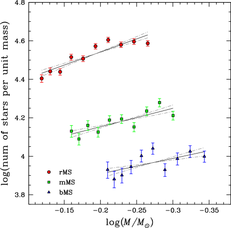
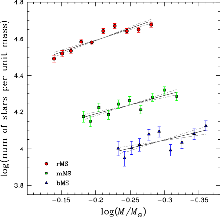
Figure 14: Mass function for the three MSs obtained by using the observed LFs of Fig. 12 and the mass-luminosity relations from Pietrinferni et al. (2004, left) and Dotter et al. (2007, right). Continuous black lines are the best-fit straight lines, while grey dotted-dash lines are the maximum- and minimum-slope lines. Note that star counts have been done in mass intervals, by dividing the numbers of stars estimated in luminosity bins by the respective bin widths in mass.

7 Discussion

The initial MF (IMF) is a fundamental characteristic of a stellar population. Similarities or differences in the IMFs of the different populations in NGC 2808 might reflect differences in the environment (primordial nebula with different composition, temperature, density, etc.) from which those populations formed. Unfortunatly, in a GC we can only measure the present-day MF, and often in a limited region of the cluster. The present-day MF can depend on several effects, including internal dynamical evolution and dynamical interaction with the Galactic gravitational potential (see e. g. Piotto & Zoccali 1999, De Marchi 2010).

In the case of a GC with multiple stellar generations, the situation is likely much more complicated, because the different populations might evolve dynamically in quite different ways. In particular, the models of D’Ercole et al. (2008) predict that a large fraction (up to 90% or more) first-generation stars should be lost early in the cluster evolution because of the expansion and stripping of the cluster’s outer layers resulting from the mass loss subsequent to SNe explosions. The possibility that first-generation stars were much more numerous at the time of cluster formation could also account for the polluting material needed to explain the He enrichment of the second (and third) generations.

For the first time, we heve presented the MFs of three different stellar generations in a GC. Unfortunately, these MFs are limited to a very small mass interval ($\leq 0.3m_{\odot}$), which in addition to the present-day mass function being the result of the cluster dynamical evolution, prevents us from drawing any conclusion about the similarities and differences among the IMFs of the different populations. We have also be unable to compare with the present day MFs of other clusters, because of both the limited mass interval sampled by our investigation and the possibility that many (or all) other clusters host multiple stellar generations, which has not been identified in previous investigations. Here, we simply note that the first-generation stars (which should be associated with the rMS, see Piotto et al. 2007) have a MF that is quite similar to the present day MFs of the other generations, and that there is marginal evidence of a possibly higher mass at which the MF starts to deviate from a uniform power law (to be investigated in greater detail) compared with the other populations.

In any case, the MFs presented in this paper provide a first observational constraint on models that describe the formation and evolution of multiple generations of stars in GCs. It will be important to extend these MFs to a larger mass interval. Another missing, but important, piece of information is the radial distribution of the different stellar populations in NGC 2808. D’Ercole et al. (2008) use hydrodynamical model to predict quite a different distribution of first- and second-generation stars. Future HST  observations using near-UV filters will be of crucial importance. The F275W and F336W bands have proven to be extremely efficient in separating different stellar populations in the MS (see, e. g. Bellini et al. 2010), whose monitoring from the cluster center to the outskirts provides us with information on the origin of the populations. The recently approved Cycle 19 HST program (GO12605; PI Piotto) will provide us with additional data to both extend the MF mass-interval coverage, and follow the radial variation in the MFs of the different stellar populations, taking advantage of the appropriate near-UV observations.

8 Summary

We have used high precision HST ACS/WFC photometry to estimate the LFs of the three MSs of NGC 2808, and measure the fraction of binaries in this GC. The field we have analyzed is located in the south-west quadrant, between $\sim 1.5$ and $\sim 6$ arcmin from the cluster center, and we have limited our study to stars with $19.5\leq{\it m}_{\rm F814W}\leq 22.0$, corresponding to $\sim 0.75\leq{\mathcal{M}}/{\mathcal{M}}_{\odot}\leq 0.44$. The present investigation represents the first attempt to measure the present day MF of different sub-populations in a Galactic GC. The main results of this paper can be summarised as follows:

1. In the studied region and luminosity (mass) interval, we have estimated a total fraction $f^{\rm BIN}\sim 0.05$ of binaries.

2. The three MSs have very similar LFs, with the number of stars increasing up to ${\it m}_{\rm F814W}\sim 20.5$, and remaining nearly constant at fainter magnitudes.

3. We made a more accurate measurement of the fraction of stars in each MS-population, finding the ratio (rMS:mMS:bMS)=(0.62:0.24:0.14) in agreement with the ratios of O-abundances along the RGB.

4. We used the mass-luminosity relations from Pietrinferni et al. (2004) and Dotter et al. (2007) to convert the observed LFs into MFs. On average, the three MFs can be represented approximately by power laws. The power law exponent, (calculated as the average of the MF slopes in the log-log diagram obtained from the two adopted mass-luminosity relations) is $\alpha=-1.2\pm 0.3$ for the rMS, $\alpha=-0.9\pm 0.3$ for the mMS, and $\alpha=-0.9\pm 0.4$ for the bMS. On the basis of the errors, the slope differences are insignificant. These slopes are consistent with the typical slope of the MF of clusters with a central concentration similar to that of NGC 2808 (De Marchi 2010). We note that the MF of the rMS seems to deviate from a power law, flattening below ${\mathcal{M}}/{\mathcal{M}}_{\rm\odot}\sim 0.6$. This effect is present independently of the adopted mass-luminosity relation. Though interesting, this result needs to be confirmed with a more extended (to smaller masses) MF.

5. Finally, this study provides accurate measurements of the fiducial lines for the three MSs (Table 1), which can be directly compared with theoretical predictions.

APPENDIX A. Effect of the binaries mass-ratio distribution on the mass functions

As already discussed in Sect. 5.2 the choice of a correct mass-ratio distribution of stars in MS-MS binary systems is crucial for a reliable estimate of the binary fraction. We have assumed in this paper that the binaries in NGC 2808 have flat distributions in f(q), consistent with the findings of Milone et al. (2011) in their study of MS-MS binaries in 59 GCs. In this Appendix, we investigate whether a different mass-ratio distribution could effect the main results of this paper.

Tout (1991) suggested that f(q) can be derived by randomly extracting secondary stars from the observed initial MF. The Hess diagram of a CMD made of binary systems only obtained by randomly extracting pair of stars from the MFs of NGC 2808 is plotted in Fig. 15 and the corresponding mass ratios are displayed in the inset.

It should be noted that Sollima et al. (2007), on the basis of their study of the binaries population in 13 GCs, suggested that the mass-ratio distribution derived from the above procedure could significantly increase the fraction of binaries with low-mass secondaries and produce a significant overestimate of the binary fraction. Furthermore, as said, the Tout (1991) distribution is also in sharp disagreement with the observed distributions of binaries with $q>0.5$ presented by Milone et al. (2011) for a sample of 59 GCs. While a precise measurement of f(q) for NGC 2808 binaries is beyond the purpose of this paper (and is not even possible with the given data set), we emphasise that in the case of binary stars formed by random associations between stars of different masses we expect a higher fraction of binaries with q$<$0.5 than can be found with the present data set.

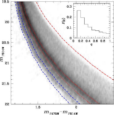
Figure 15: Hess diagram of a simulated CMD made of MS-MS binaries only. The adopted mass-ratio distribution is shown in the inset.

Once we had fixed the f(q) shape, we followed the procedure of Sects. 5 and 6 to estimate the fraction of binaries and the MFs of the three MSs. For simplicity, we used BaSTI models only. As expected, we found an higher $f^{\rm BIN}=0.09\pm 0.01$ and obtained the MFs plotted in Fig. 16. The three MFs are slightly steeper, but fully consistent within the uncertainties, with those presented in Sect. 6. In this case, we find that the rMS, the mMS, and the bMS MF have slopes of $-1.36\pm 0.24$, $-0.96\pm 0.28$, and $-1.01\pm 0.34$, respectively. These results, obtained for an ‘extreme’ f(q) demonstrate that the adopted binaries mass-ratio distribution has a small effect on the obtained MFs and does not change the main conclusions of this paper.

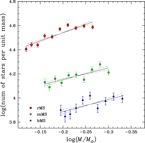
Figure 16: Mass function of the three MSs obtained by using the BaSTI mass-luminosity relations and assuming the mass-ratio distribution of MS-MS binaries shown in Fig. 15.

APPENDIX B. Effect of the binaries on the mass functions

In this work, we have assumed that both components of the binary systems have the same probability of belonging to any MS. As anticipated in the text, we explored a different extreme scenario to investigate how the membership of binaries to different MSs affects the derived MFs and the binary fraction. In this scenario, we assume that both the components, in every binary system, are taken from the same stellar population, i. e. from the same MS. The corresponding Hess diagram for a CMD made of binary systems only, is shown in Fig. 17.

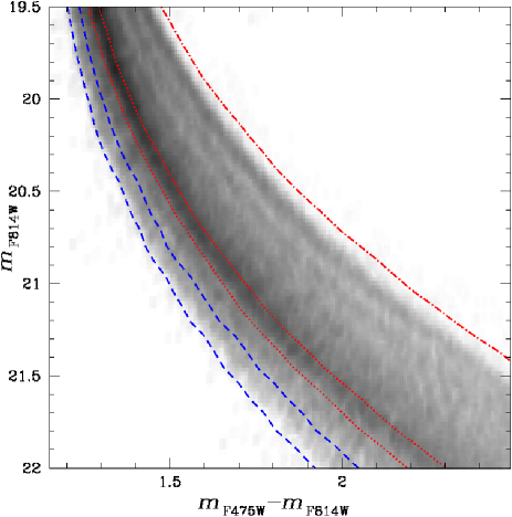
Figure 17: Hess diagram of a simulated CMD made of MS-MS binaries only. In contrast to the similar plot of Fig. 11, in this case we assumed that both components of a binary systems come from the same MS.

We adopted the same procedure described in Sects. 5 and 6 to estimate the fraction of binaries and the MFs of the three MSs. For simplicity, we used in this case only BaSTI models. The resulting value of $f^{\rm BIN}=0.05\pm 0.01$ is very close to the one obtained in Sect. 5.3 and the rMS, the mMS, and the bMS MF have similar slopes of $-1.25\pm 0.22$, $-0.87\pm 0.25$, and $-0.91\pm 0.32$, respectively, again similar to those of Sect. 6. Once again, these results suggest that the procedures adopted in this paper are insignificantly affected by the adopted scenario.

- (1) Allard F., Hauschildt P. H., Alexander D. R., & Starrfield S., 1997, ARA&A, 35, 137
- Anderson (1997) Anderson, A. J. 1997, Ph.D. Thesis,
- Anderson & King (2006) Anderson, J., & King, I. R. 2006, ACS ISR 2006-01
- Anderson et al. (2008) Anderson, J., Sarajedini, A., Bedin, L. R., et al. 2008, AJ, 135, 2055
- Anderson et al. (2009) Anderson, J., Piotto, G., King, I. R., Bedin, L. R., & Guhathakurta, P. 2009, ApJ, 697, L58
- Anderson & Bedin (2010) Anderson, J., & Bedin, L. R. 2010, PASP, 122, 1035
- Bedin et al. (2000) Bedin, L. R., Piotto, G., Zoccali, M., Stetson, P. B., Saviane, I., Cassisi, S., & Bono, G. 2000, A&A, 363, 159
- Bedin et al. (2004) Bedin, L. R., Piotto, G., Anderson, J., Cassisi, S., King, I. R., Momany, Y., & Carraro, G. 2004, ApJ, 605, L125
- Bedin et al. (2005) Bedin, L. R., Cassisi, S., Castelli, F., Piotto, G., Anderson, J., Salaris, M., Momany, Y., & Pietrinferni, A. 2005, MNRAS, 357, 1038
- Bekki & Norris (2006) Bekki, K., & Norris, J. E. 2006, ApJ, 637, L109
- Bellini et al. (2009) Bellini, A., Piotto, G., Bedin, L. R., King, I. R., Anderson, J., Milone, A. P., & Momany, Y. 2009, A&A, 507, 1393
- Bellini et al. (2010) Bellini, A., Bedin, L. R., Piotto, G., Milone, A. P., Marino, A. F., & Villanova, S. 2010, AJ, 140, 631
- Bragaglia et al. (2010) Bragaglia, A., Carretta, E., Gratton, R., D’Orazi, V., Cassisi, S., & Lucatello, S. 2010a, A&A, 519, A60
- Bragaglia et al. (2010) Bragaglia, A., Carretta, E., Gratton, R., et al. 2010b, ApJ, 720, L41
- Carretta et al. (2006) Carretta, E., Bragaglia, A., Gratton, R. G., Leone, F., Recio-Blanco, A., & Lucatello, S. 2006, A&A, 450, 523
- (16) Cassisi, S., Castellani, V., Ciarcelluti, P., Piotto, G., & Zoccali, M. 2000, MNRAS, 315, 679
- (17) Cassisi, S. 2007, Stellar Populations as Building Blocks of Galaxies, eds. A. Vazdekis and R. F. Peletier, (Cambridge: Cambridge University Press), 3
- Cassisi et al. (2008) Cassisi, S., Salaris, M., Pietrinferni, A., Piotto, G., Milone, A. P., Bedin, L. R., & Anderson, J. 2008, ApJ, 672, L115
- Dalessandro et al. (2011) Dalessandro, E., Salaris, M., Ferraro, F. R., Cassisi, S., Lanzoni, B., Rood, R. T., Fusi Pecci, F., & Sabbi, E. 2011, MNRAS, 410, 694
- D’Antona et al. (2005) D’Antona, F., Bellazzini, M., Caloi, V., Pecci, F. F., Galleti, S., & Rood, R. T. 2005, ApJ, 631, 868
- Decressin et al. (2007) Decressin, T., Charbonnel, C., & Meynet, G. 2007, A&A, 475, 859
- (22) De Marchi 2010, The Impact of HST on European Astronomy, eds. Springer, 55
- DE (08) D’Ercole, A., Vesperini, E., D’Antona, F., McMillan, S. L. W., & Recchi, S. 2008, MNRAS, 391, 825
- Dotter (07) Dotter, A., Chaboyer, B., Jevremovic, D., et al. 2007, AJ, 134, 376
- glover (07) Glover, S. C. O., & Jappsen, A.-K. 2007, ApJ, 666, 1
- Harris (1996) Harris, W. E. 1996, AJ, 112, 1487 (February 2003 update)
- Lee (09) Lee, J.-W., Kang, Y.-W., Lee, J., & Lee, Y.-W. 2009, Nature, 462, 480
- Marino et al. (2009) Marino, A. F., Milone, A. P., Piotto, G., Villanova, S., Bedin, L. R., Bellini, A., & Renzini, A. 2009, A&A, 505, 1099
- Marino et al. (2011) Marino, A. F., Villanova, S., Milone, A. P., Piotto, G., Lind, K., Geisler, D., & Stetson, P. B. 2011, ApJ, 730, L16
- Milone et al. (2008) Milone, A. P., Bedin, R. L., Piotto, G., et al. 2008, ApJ, 673, 241
- Milone et al. (2009) Milone, A. P., Bedin, L. R., Piotto, G., & Anderson, J. 2009, A&A, 497, 755
- Milone et al. (2010) Milone, A. P., Piotto, G., King, I. R, et al. 2010, ApJ, 709, 1183
- Milone et al. (2011) Milone, A. P., Piotto, G., Bedin, L., R., et al. 2011, submitted to A&A
- (34) Pietrinferni, A., Cassisi, S., Salaris, M., & Castelli, F., 2004, ApJ, 612, 168
- PZ (99) Piotto, G., & Zoccali, M. 1999, A&A, 345, 485
- Piotto et al. (2005) Piotto, G., Villanova, S., Bedin, L. R., et al. 2005, ApJ, 621, 777
- Piotto et al. (2007) Piotto, G., Bedin, L. R., Anderson J., et al. 2007, ApJ, 661, L53
- Renzini (2008) Renzini, A. 2008, MNRAS, 391, 354
- Rubenstein & Bailyn (1997) Rubenstein, E. P., & Bailyn, C. D. 1997, ApJ, 474, 701
- Shen et al. (2010) Shen, Z.-X., Bonifacio, P., Pasquini, L., & Zaggia, S. 2010, A&A, 524, L2
- Sirianni et al. (2005) Sirianni, M., Jee, M. J., Benitez, N., et al. 2005, PASP, 117, 1049
- Sollima et al. (2007) Sollima, A., Beccari, G., Ferraro, F. R., Fusi Pecci, F., & Sarajedini, A. 2007, MNRAS, 380, 781
- Sosin (1997) Sosin, C., Dorman, B., Djorgovski, S., et al. 1997, ApJ, 480, L35
- Stahler (2004) Stahler S. W. & Palla, F. 2004 The Formation of Stars, Physics Textbooks (Wiley-VCH)
- Tout (1991) Tout, C. A. 1991, MNRAS, 250, 701
- Ventura et al. (2002) Ventura, P., D’Antona, F., & Mazzitelli, I. 2002, A&A, 393, 215
- Yong et al. (2008) Yong, D., Grundahl, F., Johnson, J. A., & Asplund, M. 2008, ApJ, 684, 1159
- Zhao (2005) Zhao, B., & Bailyn, C. D. 2005, AJ, 129, 1934