Maximal Structuring of Acyclic Process Models

Abstract

This paper contributes to the solution of the problem of transforming a process model with an arbitrary topology into an equivalent structured process model. In particular, this paper addresses the subclass of process models that have no equivalent well-structured representation but which, nevertheless, can be partially structured into their maximally-structured representation. The structuring is performed under a behavioral equivalence notion that preserves observed concurrency of tasks in equivalent process models. The paper gives a full characterization of the subclass of acyclic process models that have no equivalent well-structured representation but do have an equivalent maximally-structured one, as well as proposes a complete structuring method.

Section 1 Introduction

Process models are usually represented as graphs, where nodes stand for tasks or decisions, and edges encode causal dependencies between adjacent nodes. Common process modeling notations, such as Business Process Model and Notation (BPMN) or Event-driven Process Chains (EPC), allow process models to have almost any topology. Structural freedom allows for a large degree of creativity when modeling. Nevertheless, it is often preferable that models follow certain structural patterns. A well-known property of process models is that of (well-) structuredness [1]. A model is well-structured, if for every node with multiple outgoing arcs (a split) there is a corresponding node with multiple incoming arcs (a join), such that the fragment of the model between the split and the join forms a single-entry-single-exit (SESE) process component; otherwise the model is unstructured. Figure 1 shows a process model. Each dotted box defines a component composed from the arcs that are inside or intersect the box. Split $s$ has corresponding join $z$; together they define SESE component $R1$. Yet, split $u$ has no corresponding join and, thus, the model in Figure 1 is unstructured.

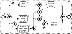
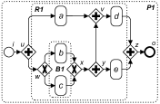
Figure 1: (a) Unstructured model, and (b) its equivalent maximally-structured version

The motivations for well-structured process modeling are manifold. Structured models are easier to layout, understand, support, and analyze [2]. Consequently, some process modeling languages urge for structured modeling, e.g., Business Process Execution Language (BPEL) and ADEPT. We advocate for a different philosophy: The modeling language should provide process modelers with a maximal degree of structural freedom to describe processes. Afterwards, scientific methods can suggest (whenever possible) alternative formalizations that are better structured, preferably well-structured.

In previous work [2], we proposed a technique to automatically transform acyclic process models with arbitrary topologies into equivalent well-structured models. The structuring is accomplished under a strong notion of behavioral equivalence called fully concurrent bisimulation [1, 2]. As an outcome, the resulting well-structured models describe the same share of concurrency as the original unstructured models. It was shown in [1] (by means of a single example) and confirmed in [2] (for the general case of acyclic models) that there exist process models that do not have an equivalent well-structured representation. Figure 1 is an example of such a model. Though not completely structurable, this model can be partially structured to result in its maximally-structured version shown in Figure 1. A process model is maximally-structured, if every model that is equivalent with it has at least the same number of SESE components defined by pairs of a split and join node as the model itself. Note that Figure 1 uses short-names for tasks $(a,b,c\ldots)$, which appear next to each task in Figure 1.

After the initial investigations in [3], this paper gives for the first time a complete solution to the problem of maximal structuring of acyclic process models. We characterize the class of acyclic process models which do not have an equivalent well-structured representation, but which can, nevertheless, be maximally structured; and we provide a complete structuring method.

The remainder of this paper proceeds as follows: The next section gives preliminary definitions. Section 3 discusses the structuring technique proposed in [2]. The technique is summarized as a chain of transformations. We define for the first time the notion of a proper complete prefix unfolding which was sketched in [2] and which is essential for obtaining sufficient behavioral information to allow maximal structuring. Section 4 devises an extension of the structuring technique for maximal structuring of process models that do not have an equivalent well-structured representation. Section 5 discusses related work and draws conclusions.

Section 2 Preliminaries

Preliminaries describe formalisms that will be used later to convey the findings.

2.1 Process Models and Nets

This section introduces all subsequently required notions on process models.

Definition 1 (Process model)

A process model $P=(A,G,C,type,\mathcal{A},\mu)$ has a non-empty set $A$ of tasks, a set $G$ of gateways, $A\cap G=\emptyset$, and a set $C\subseteq(A\cup G)\times(A\cup G)$ of control flow arcs of $P$; $\mathit{type}:G\rightarrow\{\mathit{xor},\mathit{and}\}$ assigns to each gateway a type; $\mu:A\rightarrow\mathcal{A}$ assigns to each task a name from $\mathcal{A}\neq\emptyset$.

$A\cup G$ are the nodes of $P$; a node $x\in{A\cup G}$ is a source (sink), iff $\bullet{x}=\emptyset$ (${x}\bullet=\emptyset$), where $\bullet{x}$ (${x}\bullet$) stands for the set of immediate predecessors (successors) of $x$. We assume $P$ to have a single source and a single sink task; every node of $P$ is on a path from source to sink. Each task $a\in{A}$ has at most one incoming and at most one outgoing arc, i.e., $\left|\bullet{a}\right|\leq 1\wedge\left|{a}\bullet\right|\leq 1$. Each gateway $g\in G$ is either a split ($\left|\bullet{g}\right|=1\wedge\left|{g}\bullet\right|>1$) or a join ($\left|\bullet{g}\right|>1\wedge\left|{g}\bullet\right|=1$). The semantics of process models is usually defined by a mapping to Petri nets.

Definition 2 (Petri net)

A Petri net, or a net, $N=(P,T,F)$ has finite disjoint sets $P$ of places and $T$ of transitions, and the flow relation $F\subseteq(P\times T)\cup(T\times P)$. A net system $(N,M)$ is a net $N$ with a marking $M:P\to\mathbb{N}_{0}$ assigning each $p\in P$ a number $M(p)$ of tokens in place $p$; $M_{0}$ denotes the initial marking.

For a node $x\in P\cup T$, $\bullet{x}=\{y\ |\ (y,x)\in F\}$ is a preset, whereas ${x}\bullet=\{y\ |\ (x,y)\in F\}$ is a postset of $x$; $\mathit{Min}(N)$ denotes the set of nodes of $N$ with an empty preset. For $X\subseteq P\cup T$, let $\bullet{X}=\bigcup_{x\in X}\bullet{x}$ and ${X}\bullet=\bigcup_{x\in X}{x}\bullet$. For a binary relation $R$ (e.g., $F$ or $C$), $R^{+}$ and $R^{\ast}$ denote irreflexive and reflexive transitive closures of $R$.

A net $N=(P,T,F)$ is free-choice, iff $\forall\ p\in P,|{p}\bullet|>1:\bullet{({p}\bullet)}=\{p\}$. A labeled net $N=(P,T,F,\mathcal{T},\lambda)$ has a function $\lambda:P\cup T\to\mathcal{T}$ that assigns each node a label from $\mathcal{T}$, $\tau\in\mathcal{T}$. If $\lambda(t)\neq\tau$, then $t\in T$ is observable; otherwise, $t$ is silent.

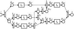
Figure 2: A WF-net that corresponds to the process model in Figure 1

Every process model (Def. 1) can be mapped to a labeled free-choice net with a special structure, called WF-net [4, 2]; the net in Figure 2 corresponds to the model in Figure 1. The execution semantics of the net (in terms of its token game) defines the semantics of the model. In our work, we require process models to be sound [5], with the intuition that a model is sound, iff its corresponding WF-system is sound.

2.2 Unfoldings

An unfolding of a net system is another net that explicitly represents all runs of the system in a possibly infinite, tree-like structure [6, 7, 8]. In [9], McMillan proposed an algorithm for the construction of a finite initial part of the unfolding, which contains full information about the reachable states of a system – a complete prefix unfolding. Next, we present main notions of the theory of unfoldings. First, we define ordering relations between pairs of nodes in a net.

Definition 3 (Ordering relations)

Let $N=(P,T,F)$ be a net, $x,y\in P\cup T$.

• $x$ and $y$ are in causal relation, written $x\leadsto_{N}y$, iff $(x,y)\in F^{+}$. $y$ and $x$ are in inverse causal relation, written $y\leftrsquigarrow_{N}x$, iff $x\leadsto_{N}y$.

• $x$ and $y$ are in conflict, $x\ \#_{N}\ y$, iff there exist distinct transitions $t_{1},t_{2}\in T$, s.t. $\bullet{t_{1}}\cap\bullet{t_{2}}\neq\emptyset$, and $(t_{1},x),(t_{2},y)\in F^{\ast}$. If $x\ \#_{N}\ x$, then $x$ is in self-conflict.

• $x$ and $y$ are concurrent, $x\ ||_{N}\ y$, iff neither $x\leadsto_{N}y$, nor $y\leadsto_{N}x$, nor $x\ \#_{N}\ y$.

The set $\mathcal{R}_{N}=\{\leadsto_{N},\leftrsquigarrow_{N},\#_{N},||_{N}\}$ forms the ordering relations of $N$.

Note that in the following we omit subscripts of ordering relations where the context is clear. A structure of an unfolding is given by an occurrence net.

Definition 4 (Occurrence net)

A net $N=(B,E,G)$ is an occurrence net, iff : for all $b\in B$ holds $|\bullet{b}|\leq 1$, $N$ is acyclic, for each $x\in B\cup E$ the set $\{y\in B\cup E\ |\ (y,x)\in G^{+}\}$ is finite, and no $e\in E$ is in self-conflict.

The elements of $B$ and $E$ are called conditions and events, respectively. Any two nodes of an occurrence net are either in causal, inverse causal, conflict, or concurrency relation [6]. An unfolding of a system is closely related to the concept of a branching process of a system. A branching process is an occurrence net where each node is mapped to a node of the system.

Definition 5 (Branching process)

A branching process of a system $S=(N,M_{0})$ is a pair $\beta=(N^{\prime},\nu)$, where $N^{\prime}=(B,E,G)$ is an occurrence net and $\nu$ is a homomorphism from $N^{\prime}$ to $N$, such that:

• the restriction of $\nu$ to $\mathit{Min}(N^{\prime})$ is a bijection between $\mathit{Min}(N^{\prime})$ and $M_{0}$, and

• for all $e_{1},e_{2}\in E$ holds if $\bullet{e_{1}}=\bullet{e_{2}}$ and $\nu(e_{1})=\nu(e_{2})$, then $e_{1}=e_{2}$.

The system $S$ is referred to as the originative system of a branching process. A branching process can be a prefix of another branching process.

Definition 6 (Prefix)

Let $\beta_{1}=(N_{1},\nu_{1})$ and $\beta_{2}=(N_{2},\nu_{2})$ be two branching processes of a system $S=(N,M_{0})$. $\beta_{1}$ is a prefix of $\beta_{2}$ if $N_{1}$ is a subnet of $N_{2}$, such that: if a condition belongs to $N_{1}$, then its input event in $N_{2}$ also belongs to $N_{1}$, if an event belongs to $N_{1}$, then its input and output conditions in $N_{2}$ also belong to $N_{1}$, and $\nu_{1}$ is the restriction of $\nu_{2}$ to nodes of $N_{1}$.

A maximal branching process of $S$ with respect to the prefix relation is called unfolding of the system. Finally, we present a complete prefix unfolding.

Definition 7 (Complete prefix unfolding)

Let $\beta=(N^{\prime},\nu)$, $N^{\prime}=(B,E,G)$, be a branching process of a system $S=(N,M_{0})$.

• A configuration $C$ of $\beta$ is a set of events, $C\subseteq E$, such that: (1) $e\in C$ implies that for all $e^{\prime}\in E$, $e^{\prime}\leadsto e$ implies $e^{\prime}\in C$, i.e., $C$ is causally closed, and (2) for all $e_{1},e_{2}\in C$ holds $\neg(e_{1}\ \#\ e_{2})$, i.e., $C$ is conflict-free.

• A local configuration of an event $e\in E$, denoted by $\left\lceil e\right\rceil$, is the set $\{e^{\prime}\in E\mid e^{\prime}\in E,e^{\prime}\leadsto e\}$, i.e., the set of events that precede $e$.

• A set of conditions of an occurrence net is a co-set if its elements are pairwise concurrent. A maximal co-set with respect to inclusion is a cut.

• For a finite configuration $C$ of $\beta$, $\mathit{Cut}(C)=(\mathit{Min}(N^{\prime})\cup{C}\bullet)\setminus\bullet{C}$ is a cut, whereas $\nu(\mathit{Cut}(C))$ is a reachable marking of $S$, denoted by $\mathit{Mark}(C)$.

• $\beta$ is complete if for each reachable marking $M$ of $S$ there exists a configuration $C$ in $\beta$, such that: (1) $\mathit{Mark}(C)=M$, i.e., $M$ is represented in $\beta$, and (2) for each transition $t$ enabled at $M$ in $N$, there exists a configuration $C\cup\{e\}$ in $\beta$, such that $e\notin C$ and $\nu(e)=t$.

• An adequate order $\lhd$ is a strict well-founded partial order on local configurations, such that $\left\lceil e\right\rceil\subset\left\lceil e^{\prime}\right\rceil$ implies $\left\lceil e\right\rceil\lhd\left\lceil e^{\prime}\right\rceil$, where $e,e^{\prime}\in E$.

• An event $e\in E$ is a cutoff event induced by $\lhd$, iff there exists a corresponding event $e^{\prime}\in E$, or $corr(e)$, such that $\mathit{Mark}(\left\lceil e\right\rceil)=\mathit{Mark}(\left\lceil e^{\prime}\right\rceil)$ and $\left\lceil e^{\prime}\right\rceil\lhd\left\lceil e\right\rceil$.

• $\beta$ is the complete prefix unfolding induced by $\lhd$, iff $\beta$ is the greatest prefix of the unfolding of $S$ that contains no event after a cutoff event.

The complete prefix unfolding is obtained by truncating the unfolding at events

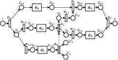
Figure 3: A complete prefix unfolding of the system in Figure 2

where the information about reachable markings starts to be redundant. Figure 3 shows a complete prefix unfolding of the system in Figure 2. In the prefix, event $e_{w}$ is a cutoff event, whereas event $e_{v}$ is its corresponding event; this relation is visualized by a dotted arrow. We write $c_{x},c^{\prime}_{x},c^{\prime\prime}_{x},\ldots\$ for conditions that are the occurrences of place $p_{x}$; correspondingly for events. The size of the prefix depends on the “quality” of the adequate order used to perform the truncation. It has been shown that the adequate order proposed in [10] results in more compact prefixes as compared to the one in [9].

Section 3 Structuring

This section discusses the technique for structuring acyclic process models, presented in [2]. We elaborate further on the technique by proposing the notion of a proper complete prefix unfolding for the first time; we will see that this prefix is essential to achieve maximal structuring.

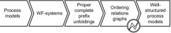
Figure 4: Structuring chain, cf., [2]

Figure 4 shows a chain of phases that collectively compose the structuring technique. The process model is decomposed into a hierarchy of process components. Each component is a process model by itself and either well-structured or unstructured. An unstructured process component can in some cases be transformed into a well-structured one. For this purpose, the component is translated into a workflow system for which the ordering relations of its tasks are derived from its proper complete prefix unfolding. If the ordering relations have certain properties, the unstructured component can be replaced by a well-structured hierarchy of smaller components that define the same ordering relations. In the following, we present each phase of the structuring in detail, whereas in the next section we extend the technique to allow maximal structuring.

3.0.1 From process models to unfoldings.

Figure 5 shows a process model that will be used in this section for explaining the structuring technique. We employ the Refined Process Structure Tree (RPST) [11, 12] to learn its structural characteristics. The RPST is built from four kinds of process components: A trivial (T) component consists of a single flow arc. A polygon (P) represents a sequence of components. A bond (B) stands for a set of components that share two common nodes – an entry and exit. Any other component is a rigid (R). A component is canonical, iff it does not overlap (on edges) with any other component. The set of all canonical process components forms a hierarchy that can be represented as a tree – the RPST. The parent of a process component is the smallest component that contains it. The root of the RPST captures the whole process model, and a leaf of the RPST is a flow arc. The dotted boxes in Figure 5 indicate the components and their hierarchy, e.g., $P1$ is a polygon which consists of trivial components $(i,s)$, $(z,o)$, and rigid $R1$. Observe that we do not explicitly visualize simple components, i.e., trivials and polygons composed of two trivials.

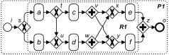
Figure 5: A process model

Polygons and bonds correspond to sequences and well-structured components of mutually-exclusive or concurrent threads. Therefore, a process model is well-structured, iff its RPST contains no rigid components. A process model can be structured by traversing its RPST bottom-up and replacing each rigid component by its equivalent well-structured component. The difficult step is to find this equivalent well-structured component.

The key idea of structuring is to refine a rigid component $R$, i.e., a node of the RPST, by a subtree of well-structured RPST nodes which define the same behavioral relations between $R$’s children. The first step when structuring a rigid component is to compute the ordering relations of its child nodes. We obtain these by constructing a complete prefix unfolding of $R$’s corresponding WF-system. The complete prefix unfolding captures information about all reachable markings of the originative system, but has a simpler structure, i.e., it is an occurrence net (Def. 4). To capture all well-structuredness contained in $R$, the complete prefix unfolding must have a specific shape called proper.

Definition 8 (Proper complete prefix unfolding)

Let $\beta=(N^{\prime},\nu)$, $N^{\prime}=(B,E,G)$, be a branching process of an acyclic system $S=(N,M_{0})$.

• A cutoff event $e\in E$ of $\beta$ induced by an adequate order $\lhd$ is healthy, iff $\mathit{Cut}(\left\lceil e\right\rceil)\setminus{e}\bullet=\mathit{Cut}(\left\lceil corr(e)\right\rceil)\setminus{corr(e)}\bullet$.

• $\beta$ is the proper complete prefix unfolding, or the proper prefix, induced by an adequate order $\lhd$, iff $\beta$ is the greatest prefix of the unfolding of $S$ that contains no event after a healthy cutoff event.

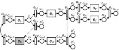
Figure 6: A proper complete prefix unfolding

Figure 6 shows a proper prefix of the system that corresponds to the rigid component $R1$ in Figure 5. A proper prefix contains all information about well-structuredness, i.e., all paired gateways of splits and joins, in a rigid in the following way. $\beta$ represents each xor split as a condition with multiple post-events; each xor join is identified by the post-conditions of a cutoff event $e$ and its corresponding event $corr(e)$, e.g., $c_{u}$ and $c_{u}^{\prime}$ in Figure 6. The notion of a cutoff event guarantees that $\beta$ contains every xor split and join. An important observation here is that corresponding pairs of xor splits and joins are always contained in the same branch of $\beta$. An and split manifests as an event with multiple post-conditions in $\beta$, whereas an and join is an event with multiple pre-conditions. The healthiness requirement on cutoff events ensures that concurrency after an and split is kept encapsulated, i.e., if several concurrent branches are introduced in the unfolding they are not truncated until the point of their synchronization, i.e., the and join. Such an intuition supports our goal to derive a well-structured process model, as bonds of a process model that define concurrency must be synchronized in the same branches of the model where they originated.

A proper complete prefix unfolding of an acyclic system is clearly finite. For structuring purposes, when computing a proper prefix, we use an adequate order proposed in [10]. This adequate order results in minimal complete prefix unfoldings for safe systems, if one only considers information about reachable markings induced by local configurations, which is the case for healthy cutoff events. Thus, the adequate order from [10] yields a minimal proper complete prefix unfolding of a safe acyclic system, which applies to our case as sound free-choice nets are safe [13].

3.0.2 From unfoldings to graphs.

The proper complete prefix unfolding of a process component $R$ contains all ordering relations of all children of $R$ in the RPST. For restructuring, $R$ (an RPST node) is to be refined into a subtree along these ordering relations. The refinement requires this information to be preserved in a hierarchically decomposable form: an ordering relations graph.

Definition 9 (Ordering relations graph)

Let $\beta=(N^{\prime},\nu)$, $N^{\prime}=(B,E,G)$, be a proper complete prefix unfolding of a sound acyclic free-choice WF-system $S=(N,M_{i})$, $N=(P,T,F,\mathcal{T},\lambda)$.

• Two nodes $x$ and $y$ of $N^{\prime}$ are in proper causal relation, denoted by $x\rightarrowtail y$, iff $(x,y)\in G^{+}$ or there exists a sequence $(e_{1},\ldots,e_{n})$ of proper cutoff events of $\beta$, $e_{i}\in E$, $1\leq i\leq n$, $n\in\mathbb{N}$, such that $(x,e_{1})\in G^{\ast}$, $(corr(e_{n}),y)\in G^{+}$, and $(corr(e_{i}),e_{i+1})\in G^{\ast}$ for $1\leq i<n$. We denote by $\leftarrowtail$ the inverse of $\rightarrowtail$.

• Let $\mathcal{R}=\{\leadsto,\leftrsquigarrow,\#,||\}$ be the ordering relations of $N^{\prime}$. The proper conflict relation of $N^{\prime}$ is $\mathord{\boxplus}=\mathord{\#}\setminus(\rightarrowtail\cup\leftarrowtail)$. The set $\mathcal{R}^{\prime}=\{\rightarrowtail,\leftarrowtail,\boxplus,||\}$ forms the proper ordering relations of $N^{\prime}$.

• We refer to $\mathcal{R}$ as observable (proper) ordering relations, iff the relations in $\mathcal{R}$ only contain pairs of events that correspond to observable transitions of $N$.

• Let $\mathcal{R}=\{\rightarrowtail,\leftarrowtail,\boxplus,||\}$ be the observable proper ordering relations of $N^{\prime}$. An ordering relations graph $\mathcal{G}=(V,A,\mathcal{B},\sigma)$ of $N^{\prime}$ has vertices $V\subseteq E$ defined by events of $\beta$ that correspond to observable transitions of $N$, arcs $A=\ \rightarrowtail\cup\ \boxplus$, and a labeling function $\sigma:V\rightarrow\mathcal{B},\mathcal{B}=\mathcal{T}\setminus\{\tau\}$ with $\sigma(v)=\lambda(\nu(v))$, $v\in V$.

Figure 7: (a),(c) Ordering relations graphs, and (b),(d) the modular decomposition trees

An ordering relations graph of a process component $R$ captures minimal and complete information about the ordering relations of events that correspond to observable transitions of a system. Figure 7 visualizes the ordering relations graph of the proper complete prefix unfolding in Figure 6. The proper causal relation $\rightarrowtail$ updates the causality relation of the prefix $\beta$ to overcome the effect of unfolding truncation, e.g., $a\rightarrowtail d$, $b\rightarrowtail f$, $d\rightarrowtail e$, etc. Figure 7 denotes that $a$ and $c$ are in proper causal relation, $a$ and $b$ are in proper conflict, whereas $e$ and $f$ are concur-

rent. Figures 7 and 7 show the graph and its MDT of the model in Figure 1.

3.0.3 From graphs to process models.

The ordering relations graph not only encodes the ordering relations, it also inherits all information about well-structuredness from the proper prefix, i.e., pairing of gateways is preserved. The structuring technique in [2] proceeds by parsing the graph into a hierarchy of subgraphs that encode ordering relations of well-structured components. The thereby discovered hierarchy of subgraphs is then used to refine a rigid component into a subtree. As shown in [2], each subgraph corresponds to the notion of a module of the modular decomposition of a directed graph [14] – thus discovering well-structuredness in the relations of an unstructured process component.

Let $\mathcal{G}=(V,A,\mathcal{B},\sigma)$ be an ordering relations graph. A module $M\subseteq V$ in $\mathcal{G}$ is a non-empty subset of vertices of $\mathcal{G}$ that are in uniform relation with vertices $V\setminus M$, i.e., if $v\in V\setminus M$, then $v$ has directed edges to all members of $M$ or to none of them, and all members of $M$ have directed edges to $v$ or none of them do. However, $v_{1},v_{2}\in V\setminus M$, $v_{1}\neq v_{2}$ can have different relations to members of $M$. Moreover, the members of $M$ and $V\setminus M$ can have arbitrary relations to each other [14]. For example, $\{e,f\}$ is a module in Figure 7. Two modules $M_{1}$ and $M_{2}$ of $\mathcal{G}$ overlap, iff they intersect and neither is a subset of the other, i.e., $M_{1}\setminus M_{2}$, $M_{1}\cap M_{2}$ , and $M_{2}\setminus M_{1}$ are all non-empty. $M_{1}$ is strong, iff there exists no module $M_{2}$ of $\mathcal{G}$, such that $M_{1}$ and $M_{2}$ overlap. The Modular Decomposition Tree (MDT) of $\mathcal{G}$ is a set of all strong modules of $\mathcal{G}$. The modular decomposition substitutes each strong module of $\mathcal{G}$ by a new vertex and proceeds recursively. The result is the MDT which is a canonical rooted tree and unique.

Now, a rigid process component $R$ of an RPST can be restructured by refining $R$ in the RPST to a subtree $T_{R}$. The root of $T_{R}$ is child of $R$’s parent, each child of $R$ is attached to a leaf of $T_{R}$, the nodes of $T_{R}$ are defined by the modules of the MDT of $R$’s ordering relations graph. The type of a node of $T_{R}$ is determined by the characteristics of its defining MDT module, as follows.

We refer to singletons of $V$ as the trivial modules of $\mathcal{G}$. Let $M$ be a non-trivial module. $M$ is complete ($C$), iff the subgraph of $\mathcal{G}$ induced by vertices in $M$ is either complete or edgeless. If the subgraph is complete, then we refer to $M$ as $xor$ complete. If the subgraph is edgeless, then we refer to $M$ as $and$ complete. $M$ is linear ($L$), iff there exists a linear order $(x_{1},\ldots,x_{|M|})$ of elements of $M$, such that there is a directed edge from $x_{i}$ to $x_{j}$ in $\mathcal{G}$, iff $i<j$. Finally, if $M$ is neither complete, nor linear, then $M$ is primitive ($P$); a primitive module is concurrent iff it contains a pair of vertices that are not connected by an edge. Figure 7 shows the MDT of the graph in Figure 7. Besides the trivial modules, the MDT contains linear $L1$, $and$ complete $C1$, and primitive $P1$. Module $L1$ is the root module, whereas trivial modules are leafs of the MDT.

An acyclic process model has an equivalent well-structured model, if its ordering relations graph contains no concurrent primitive module. According to [2], behavior captured by other module classes can be expressed by well-structured process components. A trivial module corresponds to a task. A linear module corresponds to a polygon component. An $and$ ($xor$) complete module corresponds to a bond with $and$ ($xor$) gateways as entry and exit nodes. A primitive module without concurrency can be restructured using standard compiler techniques [15].

Given all of the above, Alg. 1 summarizes the structuring technique.

Input: An acyclic process model (component) $W$

Output: A well-structured process model that is equivalent to $W$

Construct WF-net $N$ that corresponds to $W$

Construct proper complete prefix unfolding $\beta$ of $(N,M_{i})$

Construct ordering relations graph $\mathcal{G}$ of $\beta$

Compute $\mathcal{M}$ – the MDT of $\mathcal{G}$

// Construct process model $P$ by traversing $\mathcal{M}$ in postorder

foreach node $m$ of $\mathcal{M}$ do

       if $m$ is trivial then Construct a task;

      

       if $m$ is $and$ complete then Construct an $and$ bond component;

      

       if $m$ is $xor$ complete then Construct a $xor$ bond component;

      

       if $m$ is linear then Construct a trivial or polygon component;

      

       if $m$ is primitive without concurrency then

             Construct a well-structured process component using compiler techniques

      else FAIL;

      

return $P$

Algorithm 1 Structuring Acyclic Process Model (Component)

Alg. 1 traverses the MDT of an ordering relations graph of a rigid process component and constructs for each encountered module a process component from components that correspond to its child modules. The resulting hierarchy of components is the subtree that refines the rigid component.

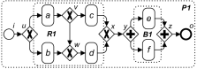
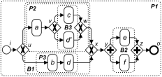
Figure 8: (a),(b) Process models that are equivalent with the process model in Figure 5

Figure 8 shows two process models that are equivalent with the process model in Figure 5. The model in Figure 8 is obtained by constructing process components that correspond to modules of the MDT in Figure 7. Here, polygon $P1$ corresponds to linear $L1$, bond $B1$ to $and$ complete $C1$, and rigid $R1$ to primitive $P1$. The model in Figure 8 is obtained from Figure 8 by structuring rigid $R1$. The structuring can be achieved by employing ID-0 transformation rule from [15].

Section 4 Maximal Structuring

Recall from Sect. 1 that a process model is maximally structured iff every equivalent model has the same number of process components defined by pairs of splits and joins as the model itself. In the light of Sect. 3, the open problem is to obtain a maximally structured process component $R$. $R$ has this property iff (1) all primitive modules in the MDT of $R$’s ordering relations graph are concurrent, and (2) there exists a bijection between non-singleton modules of the MDT and non-trivial components of the RPST which assigns to each primitive module a rigid component, to each complete a bond, and to each linear a polygon. The maximal structuredness of $R$ follows from the maximality of the modular decomposition: the ordering relations graph of $R$ inherits all information about well-structuredness from the proper complete prefix of $R$, and the MDT maximizes modules with a well-structured representation because of the decomposition into strong modules. If a primitive module $M$ with concurrency has well-structured child modules, then these modules are maximal again within $M$. Only the relations within $M$ have no structured representation as a process model, where $M$ is minimized by maximizing structuredness around and inside $M$. This yields a technique for maximal structuring: one must be able to synthesize a process component that exhibits the ordering relations described in $M$. Such a technique would allow to define unstructured process model topologies when mapping hierarchies of modules onto hierarchies of process components in Alg. 1, e.g., primitive modules in Figure 7 and Figure 7 onto rigid components in Figure 8 and Figure 1. The resulting process model would be maximally structured.

Figure 9: An extension of the structuring chain of Figure 4

In this section, we propose a solution to the synthesis problem, i.e., given an ordering relations graph (a module of an MDT) we synthesize a process model (a component of the RPST) that realizes the relations described in the graph. The solution consists of several phases that employ the results on translations between the languages of domain and net theory [16], and on folding prefixes of systems [17]. Figure 9 shows an extension of the structuring approach which was proposed in Figure 4. Next, we discuss each phase of the extension in detail.

4.0.1 From graphs to partial orders.

This section describes a translation from an ordering relations graph to a partial order of information. The partial order is an alternative formalization of the meaning of the behavior captured in the graph.

Figure 10: An ordering relations graph

The ordering relations graph in Figure 10 is the running example of Sect. 4. The graph is a primitive module with all types of relations; $d$ and $d^{\prime}$ are events with the same label.

First, we give some definitions from the theory of partially ordered sets (posets) [16]. Let $(D,\sqsubseteq)$ be a poset. For a subset $X$ of $D$, an element $y\in D$ is an upper (lower) bound of $X$, iff $x\sqsubseteq y$ ($x\sqsupseteq y$), for each element $x\in X$. An element $y\in D$ is a greatest (least) element, iff for each element $x\in D$ holds $x\sqsubseteq y$ ($x\sqsupseteq y$). An element $y\in D$ is a maximal (minimal) element, iff there exist no element $x\in D$, such that $y\sqsubset x$ ($x\sqsubset y$); $D_{max}$ and $D_{min}$ denote the sets of maximal and minimal elements of $D$. Two elements $x$ and $y$ in $D$ are consistent, written $x\uparrow y$, iff they have an upper bound, i.e., $x\uparrow y\Leftrightarrow\exists\ z\in D:x\sqsubseteq z\land y\sqsubseteq z$; otherwise they are inconsistent. A subset $X$ of $D$ is pairwise consistent, written $X^{\Uparrow}$, iff every two elements in $X$ are consistent in $D$, i.e., $X^{\Uparrow}\Leftrightarrow\forall x,y\in X:x\uparrow y$. The poset $(D,\sqsubseteq)$ is coherent, iff each pairwise consistent subset $X$ of $D$ has a least upper bound (lub) $\sqcup X$. An element $x\in D$ is a complete prime, iff for each subset $X$ of $D$, which has a lub $\sqcup X$, holds that $x\sqsubseteq\sqcup X\Rightarrow\exists\ y\in X:x\sqsubseteq y$. Let $P=(D,\sqsubseteq)$ be a poset. We write $\mathfrak{P}_{P}$ for the set of complete primes of $P$. The poset $P=(D,\sqsubseteq)$ is prime algebraic, iff $\mathfrak{P}_{P}$ is denumerable and every element in $D$ is the lub of the complete primes it dominates, i.e., $\forall\ x\in D:x=\sqcup\{y\ |\ y\in\mathfrak{P}_{P}\land y\sqsubseteq x\}$. A set $S$ is denumerable, iff it is empty or there exists an enumeration of $S$ that is a surjective mapping from the set of positive integers onto $S$.

Figure 11: (a) Poset, and (b) augmented poset obtained from Figure 10

The behavior captured in an ordering relations graph can be given as a partial order of information points. Similar to [16], the information points are chosen to be left-closed and conflict-free subsets of vertices of the graph. Each such set captures the history of events of some run of a system. Let $\mathcal{G}=(V,A,\mathcal{B},\sigma)$ be a graph and let $W$ be a subset of $V$. $W$ is conflict-free, iff $\forall\ v_{1},v_{2}\in W:(v_{1},v_{2})\nin A\lor(v_{2},v_{1})\nin A$. $W$ is left-closed, iff $\forall\ v_{1}\in W\ \forall\ v_{2}\in V:(v_{2},v_{1})\in A\land(v_{1},v_{2})\notin A\Rightarrow v_{2}\in W$. We define $\mathcal{L}[\mathcal{G}]$ as the partial order of left-closed and conflict-free subsets of $V$, ordered by inclusion. Figure 11 shows $\mathcal{L}$ of the graph in Figure 10. Thm. 4.1, inspired by Thm. 8 in [16], characterizes the posets $\mathcal{L}[\mathcal{G}]$.

Theorem 4.1

Let $\mathcal{G}=(V,A,\mathcal{B},\sigma)$ be an ordering relations graph. Then, $\mathcal{L}[\mathcal{G}]=(H,\subseteq)$ is a prime algebraic coherent partial order. Its complete primes are those elements of the form $[v]=\{v^{\prime}\in V\ |\ (v^{\prime},v)\in B^{\ast}\}$, where $B=\{a\in A\ |\ a^{-1}\notin A\}$.

Proof

Let $X\subseteq H$ be pairwise consistent. Then, $\cup X$ is conflict-free. $\sqcup X=\cup X$ and, hence, $\mathcal{L}[\mathcal{G}]$ is coherent. Each $[v]$, $v\in V$, is clearly left-closed and conflict-free. Let $X\subseteq H$ have lub $\sqcup X$. $X$ is pairwise consistent and $\sqcup X=\cup X$. Each $[v]$ is a complete prime. If $[v]\subseteq\cup X$, then $v\in\cup X$ and for some $x\in X$ holds $v\in x$ and, thus, $[v]\subseteq x$. It holds for each $X\in H$ that $X=\cup\{[v]\ |\ v\in\cup X\}$. Thus, each element of $\mathcal{L}[\mathcal{G}]$ is a lub of the complete primes below it. ∎

Given an ordering relations graph, one can construct $\mathcal{L}[\mathcal{G}]=(H,\subseteq)$ iteratively. Let $h_{1}$ and $h_{2}$ be subsets of $V$, such that $h_{2}\setminus h_{1}=\{v\}$. Then $h_{1},h_{2}\in H$, iff $h_{1}=\emptyset$ or $\exists\ a\in h_{1}:(v,a)\notin A$, and $\forall\ b\in h_{1}:(b,v)\notin A\lor(v,b)\notin A$, and $\forall\ c\in V\setminus h_{1},(c,v)\in A,(v,c)\notin A\ \exists\ d\in h_{1}:(c,d),(d,c)\in A$.

Let $\mathcal{L}[\mathcal{G}]=(H,\subseteq)$ be a partial order of an ordering relations graph. We augment $\mathcal{L}[\mathcal{G}]$ with two fresh events $i,o\notin V$. These events are designed to ensure the existence of a single source and single sink. An augmented partial order of

$\mathcal{G}$ is $\mathcal{L}^{\ast}[\mathcal{G}]=(H^{\ast},\subseteq)$, where $H^{\ast}=\emptyset\cup\{h\cup\{i\}\ |\ h\in H\}\cup\{h\cup\{i,o\}\ |\ h\in H_{max}\}$. Figure 11 shows $\mathcal{L}^{\ast}$ of the graph in Figure 10. After adding the minimal and maximal elements, the topology of posets stays unchanged, so $\mathcal{L}^{\ast}$ is a prime algebraic coherent poset.

4.0.2 From partial orders to event structures.

The next transformation step deals with translating partial orders to event structures. Event structures are intermediate concepts between partial orders and occurrence nets. The use of this intermediate concept was extensively studied in [16].

Definition 10 (Labeled event structure)

An event structure is a triple $\mathcal{E}=(E,\leq,\oplus)$, where $E$ is a set of events, $\leq$ is a partial order over $E$ called the causality relation, and $\oplus$ is a symmetric and irreflexive relation in $E$, called the conflict relation that satisfies the principle of conflict heredity, i.e., $\forall e_{1},e_{2},e_{3}\in E:e_{1}\geq e_{2}\oplus e_{3}\Rightarrow e_{1}\oplus e_{3}$. A labeled event structure $\mathcal{E}=(E,\leq,\oplus,\mathcal{C},\kappa)$ additionally has a set $\mathcal{C}$ of labels, $\tau\in\mathcal{C}$, and $\kappa:E\rightarrow\mathcal{C}$ assigns to each event a label.

An ordering relations graph $\mathcal{G}$ differs from an event structure $\mathcal{E}$ in that $\mathcal{G}$ allows violations of conflict heredity. These violations, however, are not harmful; they express equivalent runs of a system. These equivalent run are visible in posets and become explicit in event structures. A formal procedure for obtaining an event structure from a graph can be intuitively understood as unfolding of the graph. Next, we define a construction of an event structure from a poset. The definition is an extension of Def. 18 in [16]; it incorporates propagation of labels of an originative ordering relations graph to the corresponding event structure.

Definition 11 (Event structure of partial order)

Let $\mathcal{G}=(V,A,\mathcal{B},\sigma)$ be an ordering relations graph and let $P=(H,\subseteq)$ be an (augmented) prime algebraic coherent partial order of $\mathcal{G}$. Then, $\mathcal{P}[P]$ is defined as the labeled event structure $(E,\leq,\oplus,\mathcal{C},\kappa)$, where $E=\mathfrak{P}_{P}$, $\leq$ is $\subseteq$ restricted to $\mathfrak{P}_{P}$, for all $e_{1},e_{2}\in\mathfrak{P}_{P}:e_{1}\oplus e_{2}$, iff $e_{1}$ and $e_{2}$ are inconsistent in $P$, and $\mathcal{C}=\mathcal{B}\cup\{\tau\}$. Let $e\in E$, and define $\hat{e}$ as $\hat{e}\in e\setminus\bigcup_{a\subset e,a\in H}a$. Then, $\kappa(e)=\sigma(\hat{e})$, if $\hat{e}\in V$; otherwise $\kappa(e)=\tau$, for all $e\in E$.

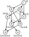
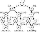
Figure 12: Event structures obtained from (a) Figure 11, and (b) poset of Figure 7

Figure 12 visualizes $\mathcal{P}[\mathcal{L}^{\ast}[\mathcal{G}]]$ for the graph $\mathcal{G}$ of Figure 10. Events are complete primes of $\mathcal{L}^{\ast}[\mathcal{G}]$ (see in boldface in Figure 11 and next to vertices in Figure 12). Directed edges encode causality (transitive dependencies are not shown), dotted edges represent implicit concurrency, whereas an absence of an edge hints at a conflict relation. The event structure in Figure 12 is structurally similar to the graph in Figure 10; they differ only in relations with fresh $i,o$ events. In general, event structures tend to have a different structure compared to the originative graphs. For instance, Figure 12 shows the event structure derived from the augmented poset of the graph in Figure 7.

4.0.3 From event structures to occurrence nets.

Nielsen et al. in [16] show a tight connection between event structures and occurrence nets. Let $N=(B,E,G)$ be an occurrence net. Then, $\xi[N]=(E,G^{\ast}\cap E^{2},\#_{N}\cap E^{2})$ is a corresponding event structure. The next theorem, borrowed from [16], defines the construction of an occurrence net from an event structure.

Theorem 4.2

Let $\mathcal{E}=(E,\leq,\oplus)$, $E\neq\emptyset$, be an event structure. Then, there exists an occurrence net $\eta[\mathcal{E}]$, such that $\mathcal{E}=\xi[\eta[\mathcal{E}]]$.

Proof

Define the set $\mathit{CE}=\{x\subseteq E\ |\ \forall e_{1},e_{2}\in x:e_{1}\neq e_{2}\Rightarrow e_{1}\ \#\ e_{2}\}$. The events

of $\eta[\mathcal{E}]$ are exactly those in $E$. The set of conditions is defined by $B=\{\left\langle e,x\right\rangle\ |\ e\in E,x\in\mathit{CE},\ and\ \forall e^{\prime}\in x:e\leq e^{\prime}\}\cup\{\left\langle 0,x\right\rangle\ |\ x\in\mathit{CE},\ and\ x\neq\emptyset\}$. The flow relation is defined by $G=\{(\left\langle e,x\right\rangle,e^{\prime})\ |\ \left\langle e,x\right\rangle\in B,e^{\prime}\in x\}\cup\{(\left\langle 0,x\right\rangle,e^{\prime})\ |\ \left\langle 0,x\right\rangle\in B,e^{\prime}\in x\}\cup\{(e,\left\langle e,x\right\rangle)\ |\ \left\langle e,x\right\rangle\in B\}$. It follows, that $\eta[\mathcal{E}]$ is an occurrence net for which $\#=\oplus$, and hence $\xi[\eta[\mathcal{E}]]=\mathcal{E}$. ∎

Figure 13 shows the occurrence net which is constructed from the event structure shown in Figure 12 using the principles of Thm. 4.2. Thm. 4.2 defines a “maximal” construction, cf., [16], i.e., the resulting nets tend to contain much redundancy. With Def. 12 we aim at preserving only essential behavioral dependencies.

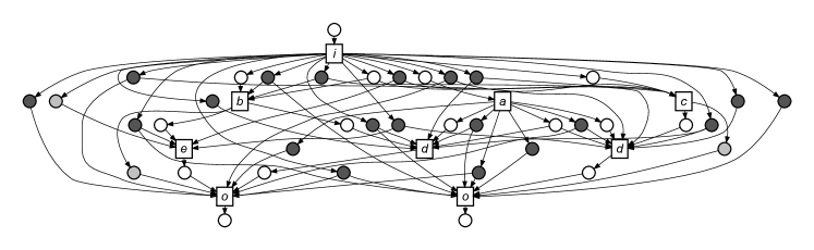
Figure 13: Occurrence net obtained from Fig. 12 by Thm. 4.2.

Definition 12 (Conditions)

Let $N=(B,E,G)$ be an occurrence net.

• A condition $b\in B$ is redundant, iff ${b}\bullet=\emptyset\land\exists\ b^{\prime}\in B,b\neq b^{\prime}:b^{\prime}\in{(\bullet{b})}\bullet$ or $\bullet{b}=\emptyset\land\exists\ b^{\prime}\in B,b\neq b^{\prime}:({b}\bullet={b^{\prime}}\bullet)\land(\bullet{b^{\prime}}\neq\emptyset)$.

• A condition $b\in B$ is subsumed by condition $b^{\prime}\in B$, $b\neq b^{\prime}$, iff $\bullet{b}=\bullet{b^{\prime}}\land{b}\bullet\subseteq{b^{\prime}}\bullet$.

• A condition $b\in B$ denotes a transitive conflict between events $e,e^{\prime}\in E$, iff $\exists\ b^{\prime}\in B,b\neq b^{\prime}\ \exists\ e^{\prime\prime}\in{b^{\prime}}\bullet,e\neq e^{\prime\prime}\neq e^{\prime}:\bullet{b}=\bullet{b^{\prime}}\land e^{\prime}\in{b}\bullet\cap\ {b^{\prime}}\bullet\land\ e\in{b}\bullet\land\ e\leadsto_{N}e^{\prime\prime}$.

• Any other condition is required.

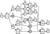
Figure 14: Simplified occurrence net obtained from Figure 13

A redundant condition has no pre-event (post-event), and is not a pre-condition (post-condition) of the initial (a final) event. A subsumed condition $b$ always has a sibling $b^{\prime}$ expressing the same constraints for larger set of events; depicted light-grey in Figure 13. A condition $b$ denotes a transitive conflict between two events, if an “earlier” condition $b^{\prime}$ already denotes this conflict; depicted dark-grey in Figure 13. All these conditions can be removed from the occurrence net without loosing information about ordering of events. For our structuring, we remove from an occurrence net all redundant and all subsumed conditions, and all transitive conflicts which have at least two post-events. Removing these conditions from the net in Figure 13 yields the net in Figure 14. Note that all conditions are labeled $\tau$, and that transitive conflicts with one post-event will be needed for the next step.

4.0.4 From occurrence nets to nets.

The simplified occurrence net obtained by Thm. 4.2 and Def. 12 is already a process model – though one with duplicate structures and multiple sinks. We obtain a more compact model with a single sink by folding the occurrence net. Intuitively, we fold any two nodes of an occurrence

net which have isomorphic successors into one node. This operation preserves all ordering relations and all behavior represented in the net. Folding finite occurrence nets succeeds with the following inductive definition of a future equivalence.

Definition 13 (Future equivalence, Folded net)

Let $N=(B,E,G,\mathcal{T},\lambda)$ be a labeled occurrence net, $\forall\ b\in B:\lambda(b)=\tau$. An equivalence relation $\sim_{f}$ is a future equivalence on $N$, iff there exists an equivalence $\mathord{\sim}\subseteq(B\times B)\cup(E\times E)$:

• For all $b,b^{\prime}\in B$, if ${b}\bullet={b^{\prime}}\bullet$, then $b\sim b^{\prime}$.

• For $X,Y\subseteq B\cup E$, write $X\sim Y$, iff $X=\{x_{1},\ldots,x_{k}\},Y=\{y_{1},\ldots,y_{k}\}$, s.t. $x_{i}\sim y_{i}$, for $1\leq i\leq k$;

• For all $x,y\in B\cup E$, if $\lambda(x)=\lambda(y)$ and ${x}\bullet\sim{y}\bullet$ and $\neg(x\mathrel{||}_{N}y)$, then $x\sim y$.

The future equivalence defines $x\sim_{f}y$, iff $x\sim y\wedge(x,y\in E\Rightarrow\bullet{x}\sim\bullet{y})$.
Let $\sim_{f}$ be a future equivalence on $N$; write $\langle x\rangle_{f}=\{y\mid y\sim_{f}x\}$ for the equivalence class of $x$. Then the folded net of $N$ under $\sim_{f}$ is the net $N_{f}=(\{\langle b\rangle_{f}\mid b\in B\},\{\langle e\rangle_{f}\mid e\in E\},\{(\langle x\rangle_{f},\langle y\rangle_{f})\mid(x,y)\in F\},\lambda_{f})$ with $\lambda_{f}(\langle x\rangle_{f})=\lambda(x)$.

Considering the occurrence net $N$ in Figure 14, the equivalence $\sim_{f}$ with the classes $\{b_{14},b_{15}\}$, $\{e_{8},e_{9}\}$, $\{b_{9},b_{11}\}$, $\{b_{12},b_{13}\}$, $\{e_{6},e_{7}\}$, $\{b_{6},b_{8}\}$, and all other nodes remaining singleton, is a future equivalence on $N$. Folding $N$ under $\sim_{f}$ yields the net in Figure 15. Folding $N$ into $N_{f}$ preserves the behavior of $N$, cf., [17, Thm. 8.7].

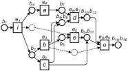
Figure 15: Folded net obtained from Figure 14

Each occurrence net has several future equivalences differing in how pre-conditions of events are folded. A simple algorithm to compute a future equivalence implements the steps of Def. 13 and uses branching and backtracking whenever for a condition $b$ there are two or more pairwise concurrent conditions that could be folded with $b$. Each option is explored and the most-compact folding is chosen. For instance, after folding $b_{14}\sim_{f}b_{15}$ and $e_{8}\sim_{f}e_{9}$, for $b_{13}$ the folding options $b_{12}$ and $b_{9}$ can be explored; backtracking yields $b_{12}$ as the better match for $b_{13}$ because of their $d$-labeled pre-events. Various heuristics improve exploration and backtracking.

If the original process model has control-flow edges between gateways without any visible activity, folding gets more involved. In this case, the occurrence net contains supposedly equivalent events with different numbers of required pre-conditions, e.g., $e_{8}$ and $e_{9}$ with required pre-conditions $\{b_{12}\}$ and $\{b_{11},b_{13}\}$, respectively. Fortunately, Thm. 4.2 encodes all possible invisible control-flow edges as transitive conflicts with one post-event (grey-shaded conditions in Figure 14). When extending the future equivalence to pre-conditions of events, a subset of these transitive conflicts needs to be taken into account as follows:

• Pick the largest set $B^{\prime}$ of required pre-conditions, e.g., $b_{11}$ and $b_{13}$.

• For each $b\in B^{\prime}$, extend the folding equivalence with a required condition or a transitive conflicts, e.g., $b_{13}\sim_{f}b_{12}$, $b_{11}\sim_{f}b_{9}$.

• Finally, remove all transitive conflicts not required in this step, e.g., $b_{10}$.

Applying this procedure on our example yields the folded net shown in Figure 15 without the dashed conditions and arcs.

4.0.5 From nets to process models.

The folding was the second to last step in synthesizing a process model from a given ordering relations graph. We obtained a Petri net $N_{f}$ which we now transform into a process model $P$.

The initial transition $i$ (final transition $o$) is mapped to the start (end) node of $P$. Every other transition of $N_{f}$ becomes a task of $P$. Gateways of $P$ follow

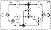
Figure 16: Process model obtained from Figure 15

from non-singleton pre- and postsets of nodes of $N_{f}$. A transition $t$ with two or more pre-places is preceded by an $and$ join; two or more post-places of $t$ define an $and$ split; the pre- and postsets of places define $xor$ splits and joins, respectively; $and$ gateways are always positioned closer to the task. In our example, ${e_{1}}\bullet$ defines $and$ split $s$ in Figure 16, ${b_{2}}\bullet$ defines $xor$ split $u$, ${e_{3}}\bullet$ defines $and$ split $v$, $\bullet{\langle e_{6},e_{7}\rangle}$ defines $and$ join $t$, and $\bullet{\langle b_{6},b_{8}\rangle}$ defines $xor$ join $x$ positioned between $t$ and $v$ ($and$ gateways closer to tasks); correspondingly for all other gateways. The arc from $e_{2}$ to $\langle b_{9},b_{11}\rangle$ which was obtained from a transitive conflict (Def. 12) results in an important control-flow arc from $w$ to $y$ without any task.

Section 5 Related Work and Conclusion

In this paper, we addressed the problem of structuring acyclic process models. It is well known that any flowchart can be structured [15], but the same claim does not apply for process models comprising concurrency [1]. Some works have been devoted to the characterization of sources of unstructuredness [18, 19] and to development of methods for structuring process models with concurrency [20, 21]. In [2], we presented the first full characterization of the class of acyclic process models that have an equivalent structured version along with a structuring method. The method stops when the input model contains an inherently unstructured fragment. This paper completes the approach by providing a method to synthesize the fragments corresponding to inherently unstructured parts of the input model.

Close to our setting, the problem of synthesizing nets from behavioral specifications has been a line of active research for about two decades [22, 23]. This area has given rise to a rich body of knowledge and to a number of tools, e.g., petrify [22] and viptool [23]. Yet, these solutions fail in our setting: petrify aims at maximizing concurrency while our synthesis preserves given concurrency, viptool synthesizes nets with arc weights, which do not map to process models.

The approach is implemented in a tool, namely bpstruct, which is publicly available at http://code.google.com/p/bpstruct. The running time of our structuring technique is mostly dominated by the time required to compute proper prefixes, which for safe systems is $O((|B|/n)^{n})$ [10], where $B$ is the set of conditions of the prefix and $n$ is the maximal size of the presets of the transitions in the originative system. All other steps can be accomplished in linear time. Concerning the extension for maximal structuring, the theoretic discussion in this paper implies exponential time and space complexity when constructing posets (this is due to our wish to be close to the existing theory). However, in practice, given an ordering relations graph one can construct a poset which only contains information from the graph, without introducing duplicate events, and thus stay linear to the size of the graph. At the theoretical level this requires introduction of a concept of a cutoff for posets followed by an adjustment of the theories along subsequent transformation steps. The folding step is a reverse of unfolding and, thus, in the best case can be performed in the same time. The fact that the running time depends on the size of the result, allows introduction

of a heuristic to terminate computation if the result gets large, e.g., the event duplication factor is larger than two. However, in practice we have never observed such a need with our implementation always delivering the result in milliseconds. Our ongoing work aims at extending the method to handle models with loops.

References

- [1] Kiepuszewski, B., ter Hofstede, A.H.M., Bussler, C.: On structured workflow modelling. In: CAiSE. Volume 1789 of LNCS., Springer (2000) 431–445
- [2] Polyvyanyy, A., García-Bañuelos, L., Dumas, M.: Structuring acyclic process models. In: BPM. Volume 6336 of LNCS., Springer (2010) 276–293
- [3] Elliger, F., Polyvyanyy, A., Weske, M.: On separation of concurrency and conflicts in acyclic process models. In: EMISA. Volume 172 of LNI., GI (2010) 25–36
- [4] Kiepuszewski, B., ter Hofstede, A.H.M., van der Aalst, W.M.P.: Fundamentals of control flow in workflows. Acta Inf. 39(3) (2003) 143–209
- [5] van der Aalst, W.M.P.: Verification of workflow nets. In: ATPN. Volume 1248 of LNCS., Springer (1997) 407–426
- [6] Nielsen, M., Plotkin, G.D., Winskel, G.: Event structures and domains. Theoretical Computer Science 13(1) (1980) 85–108
- [7] Engelfriet, J.: Branching processes of Petri nets. Acta Inf. 28(6) (1991) 575–591
- [8] Esparza, J., Heljanko, K.: Unfoldings – A Partial-Order Approach to Model Checking. EATCS Monographs in Theoretical Computer Science. Springer (2008)
- [9] McMillan, K.L.: A technique of state space search based on unfolding. FMSD 6(1) (1995) 45–65
- [10] Esparza, J., Römer, S., Vogler, W.: An improvement of McMillan’s unfolding algorithm. FMSD 20(3) (2002) 285–310
- [11] Polyvyanyy, A., Vanhatalo, J., Völzer, H.: Simplified computation and generalization of the refined process structure tree. In: WS-FM. Volume 6551 of LNCS. (2010)
- [12] Vanhatalo, J., Völzer, H., Koehler, J.: The refined process structure tree. DKE 68(9) (2009) 793–818
- [13] van der Aalst, W.M.P.: Workflow verification: Finding control-flow errors using Petri-net-based techniques. In: BPM. Volume 1806 of LNCS. (2000) 161–183
- [14] McConnell, R.M., de Montgolfier, F.: Linear-time modular decomposition of directed graphs. Discrete Applied Mathematics 145(2) (2005) 198–209
- [15] Oulsnam, G.: Unravelling unstructured programs. Comput. J. 25(3) (1982) 379–387
- [16] Nielsen, M., Plotkin, G.D., Winskel, G.: Petri nets, event structures and domains, Part I. Theor. Comput. Sci. 13 (1981) 85–108
- [17] Fahland, D.: From Scenarios To Components. PhD thesis, Humboldt-Universität zu Berlin and Technische Universiteit Eindhoven (2010)
- [18] Liu, R., Kumar, A.: An Analysis and Taxonomy of Unstructured Workflows. In: BPM. Volume 3649 of LNCS. (2005) 268–284
- [19] Polyvyanyy, A., García-Bañuelos, L., Weske, M.: Unveiling Hidden Unstructured Regions in Process Models. In: OTM. Volume 5870 of LNCS. (2009) 340–356
- [20] Hauser, R., Koehler, J.: Compiling Process Graphs into Executable Code. In: GPCE. Volume 3286 of LNCS. (2004) 317–336
- [21] Hauser, R., Friess, M., Küster, J.M., Vanhatalo, J.: An Incremental Approach to the Analysis and Transformation of Workflows Using Region Trees. IEEE Transactions on Systems, Man, and Cybernetics, Part C 38(3) (2008) 347–359
- [22] Cortadella, J., Kishinevsky, M., Lavagno, L., Yakovlev, A.: Deriving Petri Nets for Finite Transition Systems. IEEE Trans. Computers 47(8) (1998) 859–882
- [23] Bergenthum, R., Desel, J., Mauser, S.: Comparison of different algorithms to synthesize a Petri net from a partial language. TOPNOC 3 (2009) 216–243