Single-Particle Spectral Density of a Bose Gas in the Two-Fluid Hydrodynamic Regime

Abstract

In Bose supefluids, the single-particle Green’s function can be directly related to the superfluid velocity-velocity correlation function in the hydrodynamic regime. An explicit expression for the single-particle spectral density was originally written down by Hohenberg and Martin in 1965, starting from the two-fluid equations for a superfluid. We give a simple derivation of their results. Using these results, we calculate the relative weights of first and second sound modes in the single-particle spectral density as a function of temperature in a uniform Bose gas. We show that the second sound mode makes a dominant contribution to the single-particle spectrum in relatively high temperature region. We also discuss the possibility of experimental observation of the second sound mode in a Bose gas by photoemission spectroscopy.

I Introduction

In the low-frequency dynamics of superfluid Bose and Fermi atomic gases, the most dramatic effects related to superfluidity are described by Landau’s two-fluid hydrodynamics analogous to the case of liquid ⁴He Griffin et al. (2009). These equations only describe the dynamics when collisions are sufficiently strong to produce a state of local thermodynamic equilibrium Landau (1941). This requirement is usually summarized as $\omega\tau\ll 1$, where $\omega$ is the frequency of a collective mode and $\tau$ is the appropriate relaxation rate. In this regime two sound modes can be distinguished: the first sound mode consists of an in-phase oscillation of the superfluid and normal fluid components, while the second sound mode consists of an out-of-phase oscillation of the superfluid and normal fluid components. The occurrence of two distinct modes arises from the presence of both a superfluid component and normal fluid component, which are coupled to each other. Recently, there has been renewed interest in second sound mode in superfluid Bose and Fermi gases Heiselberg (2006); Capuzzi et al. (2006); Joseph et al. (2007); Meppelink et al. (2009); Hu et al. (2010). The study of ultracold gases in collisional hydrodynamic regime has been difficult because the density and the $s$-wave scattering length are typically not large enough. However, Feshbach resonances allow ones to achieve conditions where the Landau two-fluid description is correct. Recent experiments have begun to observe sound propagation in trapped superfluid Fermi gases with a Feshbach resonance Kinast et al. (2004); Bartenstein et al. (2004); Joseph et al. (2007). At unitarity, the magnitude of the $s$-wave scattering length that characterizes the interactions between fermions in different hyperfine states diverges ($|a_{s}|\to\infty$). Owing to the strong interaction close to unitarity, the dynamics of superfluid Fermi gases with a Feshbach resonance at finite temperatures are expected to be described by Landau’s two-fluid hydrodynamic equations Massignan et al. (2005); Hu et al. (2010).

More recently, sound propagation in a Bose-condensed gas in a highly elongated (cigar-shaped) trap has been observed in Ref. Meppelink et al. (2009), where the thermal cloud is in the hydrodynamic regime and thus the system is described by the two-fluid model. In this experiment, the sound wave in a highly elongated trapped gas can be excited by a sudden modification of a trapping potential using the focused laser beam. The resulting density perturbations propagate with a speed of sound. This experimental work has reported some success, with evidence for a second sound mode in superfluid Bose gases, but first sound mode was not observed. In order to clearly demonstrate the two fluid dynamics of superfluids, it will be important to observe both first and second sound modes. In the case of a sound wave excited by a sudden modification of a trapping potential, the thermal density perturbations (first sound) is so small that one cannot distinguish small density perturbations from signal-to-noise in the thermal cloud in this regime Meppelink et al. (2009).

In general, the single-particle Green’s function of Bose superfluids in the low-frequency, long-wavelength regime is directly related to the superfluid velocity-velocity correlation function Hohenberg and Martin (1965), which is therefore coupled to first and second sound modes. Making use of this exact relation, In this paper, we propose that first and second sound can be probed by measuring the single-particle spectral density. This type of quantity is directory related to the tunneling current spectroscopy Luxat and Griffin (2002). Resent experience on ultracold Fermi gases by JILA group Stewart et al. (2008) showed that the momentum-resolved photoemission-type spectroscopy is a powerful technique to directly probe single-particle excitations of ultracold atomic gases.

In Sec. II, we discuss the relation between superfluid velocity-velocity correlation function and the single-particle Green’s function of Bose superfluids, which was discussed by Hohenberg and Martin (which will be referred to as “HM”)  Hohenberg and Martin (1965). We also give a simple derivation of the explicit expression for the single-particle Green’s function in the two-fluid hydrodynamic regime, following the approach analogous to the derivation of the density correlation function given in Ch.14 of Ref. Griffin et al. (2009).

In Sec. III, we calculate the relative weights of first and second sound mode in the single-particle spectral density. For this purpose, we use the Hartree-Fock-Bogoliubov (HFB)-Popov approximation Griffin (1996), for calculating various thermodynamic variables. We also compare the relative weights of first and second sound modes in both the single-particle spectral density and the dynamic structure factor

In Sec. IV, We show the single-particle spectral density in connection with the rf-tunneling current spectroscopy Törmä and Zoller (2000); Tsuchiya et al. (2010); Luxat and Griffin (2002). We will show that both first and second sound mode can be observed by photoemission-type spectroscopy. For comparison, we also show the he single-particle spectral density in the collisionless limit using the HFB-Popov approximation.

II Superfluid velocity-velocity correlation function and the single-particle Green’s function

According to HM theory, the superfluid velocity-velocity correlation function in the non-dissipative hydrodynamic limit is given by Hohenberg and Martin (1965)

$$\chi_{v_{s},v_{s}}({\bf q},\omega)=\frac{\left(\rho_{s}\lambda_{v_{s},v_{s}}\omega^{2}-u_{1}^{2}u_{2}^{2}q^{2}\right)q^{2}}{\rho_{s}(\omega^{2}-u_{1}^{2}q^{2})(\omega^{2}-u_{2}^{2}q^{2})},$$ (1)

where $u_{1}$ and $u_{2}$ are first and second sound velocities, which satisfy $u_{1}^{2}u_{2}^{2}=\frac{T\rho_{s}\bar{s}^{2}}{\rho_{n}c_{v}}\frac{\partial P}{\partial\rho}{\bigg{|}}_{T}$. Here $\rho_{s}$ and $\rho_{n}$ are superfluid and normal fluid densities and $\bar{s}$ is the entropy per unit mass. The explicit expression for $\lambda_{v_{s},v_{s}}$ is given by

$$\lambda_{v_{s},v_{s}}=\frac{1}{\rho}\left[\left(\frac{\partial P}{\partial\rho}\right)_{\bar{s}}-2\frac{T}{c_{v}}\frac{\bar{s}}{\rho}\left(\frac{\partial P}{\partial T}\right)_{\rho}+\frac{T\bar{s}^{2}}{c_{v}}\right]$$ (2)

In the low-frequency region, the single-particle Green’s function $G({\bf q},\omega)$ is related to the superfluid velocity-velocity correlation function through Hohenberg and Martin (1965)

$$G({\bf q},\omega)=\frac{n_{0}m^{2}}{q^{2}}\chi_{v_{s},v_{s}}({\bf q},\omega),$$ (3)

where $n_{0}$ is the condensate density. The single-particle spectral density $A({\bf q},\omega)$ is related to the Green’s function $G({\bf q},\omega)$ through

$$G({\bf q},\omega)=\int_{-\infty}^{\infty}\frac{d\omega}{2\pi}\frac{A({\bf q}.\omega)}{\omega^{\prime}-\omega}$$ (4)

This gives

$$A({\bf q},\omega) =\frac{2\pi n_{0}m^{2}}{\rho_{s}}{\rm sgn}(\omega)\left[\frac{u_{1}^{2}\rho_{s}\lambda_{v_{s},v_{s}}-u_{1}^{2}u_{2}^{2}}{u_{1}^{2}-u_{2}^{2}}\delta(\omega^{2}-u_{1}^{2}q^{2})+\frac{u_{2}^{2}\rho_{s}\lambda_{v_{s},v_{s}}-u_{1}^{2}u_{2}^{2}}{u_{1}^{2}-u_{2}^{2}}\delta(\omega^{2}-u_{2}^{2}q^{2})\right]$$

$$=\frac{\pi n_{0}m^{2}}{\rho_{s}q}\Bigg{\{}X_{1}\left[\delta(\omega-u_{1}q)-\delta(\omega+u_{1}q)\right]+X_{2}\left[\delta(\omega-u_{2}q)-\delta(\omega+u_{2}q)\right]\Bigg{\}},$$ (5)

where $X_{1}$ and $X_{2}$ are defined by

$$X_{1}\equiv\frac{u_{1}(\rho_{s}\lambda_{v_{s},v_{s}}-u_{2}^{2})}{u_{1}^{2}-u_{2}^{2}},~{}~{}~{}X_{2}\equiv\frac{u_{2}(\rho_{s}\lambda_{v_{s},v_{s}}-u_{1}^{2})}{u_{1}^{2}-u_{2}^{2}}.$$ (6)

HM gives a systematic way to calculate various correlations functions in uniform superfluids in the two-fluid hydrodynamic regime. However, their detailed derivation is quite involved, which closely follows the the earlier paper by Kadanoff and Martin Kadanoff and Martin (1963) on a normal fluid. In this section, we give an alternative derivation, analogous to Sec.14.3 of Ref. Griffin et al. (2009) for the density-density correlation function. We start with the non-dissipative two-fluid hydrodynamic equations:

$$\frac{\partial n}{\partial t}+\nabla\cdot{\bf j}=0,$$ (7)

$$m\frac{\partial{\bf j}}{\partial t}=-\nabla P,$$ (8)

$$m\frac{\partial{\bf v}_{s}}{\partial t}=-\nabla\left(\mu+\frac{mv_{s}^{2}}{2}\right),$$ (9)

$$\frac{\partial s}{\partial t}+\nabla\cdot(s{\bf v}_{n})=0.$$ (10)

The total mass density and mass current are given by the sum of two components

$$mn\equiv\rho=\rho_{s}+\rho_{n},$$ (11)

$$m{\bf j}\equiv\rho_{s}{\bf v}_{s}+\rho_{n}{\bf v}_{n}.$$ (12)

To calculate the superfluid velocity-velocity correlation function, we add a time-dependent external current $\delta{\bf j}_{\rm ex}({\bf r},t)$ that is only coupled to the superfluid velocity ${\bf v}_{s}$. That is, the continuity equation becomes

$$\frac{\partial n}{\partial t}+\nabla\cdot{\bf j}+\nabla\cdot\delta{\bf j}_{\rm ex}=0,$$ (13)

where as the entropy equation (10) is unchanged.

Taking time derivative of (13) Cwe obtain

$$\frac{\partial^{2}\rho}{\partial t^{2}}=-m\nabla\cdot\left(\frac{\partial{\bf j}}{\partial t}+\frac{\partial\delta{\bf j}_{\rm ex}}{\partial t}\right)=\nabla^{2}P-m\nabla\cdot\frac{\partial\delta{\bf j}_{\rm ex}}{\partial t}$$ (14)

Taking time derivative of (10) and linearize it in fluctuations, we obtain

$$\frac{\partial^{2}\delta s}{\partial t^{2}}=-s_{0}\nabla\cdot\frac{\partial{\bf v}_{n}}{\partial t}$$ (15)

One can show that

$$\rho_{n0}\frac{\partial\delta{\bf v}_{n}}{\partial t}=-\frac{n_{n0}}{n_{0}}\nabla\delta P-\frac{n_{s0}}{n_{0}}s_{0}\nabla\delta T$$ (16)

and thus

$$\frac{\partial^{2}\delta s}{\partial t^{2}}=\frac{s_{0}}{\rho_{0}}\nabla^{2}\delta P+\frac{s_{0}^{2}}{\rho_{0}}\left(\frac{\rho_{s0}}{\rho_{n0}}\right)\nabla^{2}\delta T$$ (17)

This is the same as in the case without the external current, since the derivation does not involve the continuity equation. It can be rewritten in terms of the local entropy per unit mass $\bar{s}=s/\rho$. Using

$$\delta\bar{s}=-\frac{s_{0}}{\rho_{0}^{2}}\delta\rho+\frac{1}{\rho_{0}}\delta s,$$ (18)

we see that

$$\frac{\partial^{2}\delta\bar{s}}{\partial t^{2}}=-\frac{s_{0}}{\rho_{0}^{2}}\frac{\partial^{2}\delta\rho}{\partial t^{2}}+\frac{1}{\rho_{0}}\frac{\partial^{2}\delta s}{\partial t^{2}}$$ (19)

Using (14) and (17) in (19), we obtain

$$\frac{\partial^{2}\delta\bar{s}}{\partial t^{2}} = -\frac{s_{0}}{\rho_{0}^{2}}\left(\nabla^{2}\delta P-m\nabla\cdot\frac{\partial\delta{\bf j}_{\rm ex}}{\partial t}\right)+\frac{1}{\rho_{0}}\left[\frac{s_{0}}{\rho_{0}}\nabla^{2}\delta P+\frac{s_{0}^{2}}{\rho_{0}}\left(\frac{\rho_{s0}}{\rho_{n0}}\right)\nabla^{2}\delta T\right]$$ (20)

$$= \bar{s}_{0}^{2}\left(\frac{\rho_{s0}}{\rho_{n0}}\right)\nabla^{2}\delta T+\frac{\bar{s}_{0}}{n_{0}}\nabla\cdot\frac{\partial\delta{\bf j}_{\rm ex}}{\partial t}$$

Let us now use $P$ and $T$ as independent variables. We thus express fluctuations of $\rho$ and $s$ in terms of $P$ and $T$ as

$$\delta\rho=\left(\frac{\partial\rho}{\partial P}\right)_{T}\delta P+\left(\frac{\partial\rho}{\partial T}\right)_{P}\delta T$$ (21)

$$\delta\bar{s}=\left(\frac{\partial\bar{s}}{\partial P}\right)_{T}\delta P+\left(\frac{\partial\bar{s}}{\partial T}\right)_{P}\delta T$$ (22)

We then obtain

$$\left(\frac{\partial\rho}{\partial P}\right)_{T}\frac{\partial^{2}\delta P}{\partial t^{2}}+\left(\frac{\partial\rho}{\partial T}\right)_{P}\frac{\partial^{2}\delta T}{\partial t^{2}}-\nabla^{2}P=-m\nabla\cdot\frac{\partial\delta{\bf j}_{\rm ex}}{\partial t}$$ (23)

$$\left(\frac{\partial\bar{s}}{\partial P}\right)_{T}\frac{\partial^{2}\delta P}{\partial t^{2}}+\left(\frac{\partial\bar{s}}{\partial T}\right)_{P}\frac{\partial^{2}\delta T}{\partial t^{2}}-\bar{s}_{0}^{2}\left(\frac{\rho_{s0}}{\rho_{n0}}\right)\nabla^{2}\delta T=\frac{\bar{s}_{0}}{n_{0}}\nabla\cdot\frac{\partial\delta{\bf j}_{\rm ex}}{\partial t}$$ (24)

We consider an external current that excites modes of frequency $\omega$ and wavevector ${\bf q}$, namely

$$\delta{\bf j}_{\rm ex}({\bf r},t)=\delta{\bf j}_{\rm ex}({\bf q},\omega)e^{i({\bf q}\cdot{\bf r}-\omega t)},$$ (25)

and look at the plane-wave solutions of Eqs.(23),(24)

$$\delta P({\bf r},t)=\delta P_{{\bf q},\omega}e^{i({\bf q}\cdot{\bf r}-\omega t)},~{}~{}\delta T({\bf r},t)=\delta T_{{\bf q},\omega}e^{i({\bf q}\cdot{\bf r}-\omega t)}.$$ (26)

This gives two coupled algebraic equations

$$\left(\begin{array}[]{c}\delta P_{{\bf q},\omega}\\[22.76219pt] \delta T_{{\bf q},\omega}\end{array}\right)\left(\begin{array}[]{cc}\displaystyle\left(\frac{\partial\rho}{\partial P}\right)_{T}\omega^{2}-q^{2}&\displaystyle\left(\frac{\partial\rho}{\partial T}\right)_{P}\omega^{2}\\[14.22636pt] \displaystyle\left(\frac{\partial\bar{s}}{\partial P}\right)_{T}\omega^{2}&\displaystyle\left(\frac{\partial\bar{s}}{\partial T}\right)_{P}\omega^{2}-\bar{s}_{0}^{2}\left(\frac{\rho_{s0}}{\rho_{n0}}\right)q^{2}\end{array}\right)=\left(\begin{array}[]{c}1\\[22.76219pt] \displaystyle-\frac{\bar{s}_{0}}{\rho_{0}}\end{array}\right)m\omega{\bf q}\cdot\delta{\bf j}_{\rm ex}({\bf q},\omega)$$ (27)

We note that the determinant of the coefficient matrix is given by

$$D(q,\omega)=\left[\left(\frac{\partial T}{\partial\bar{s}}\right)_{\rho}\left(\frac{\partial P}{\partial\rho}\right)_{T}\right]^{-1}$$

$$\times\left\{\omega^{4}-\left[\left(\frac{\partial P}{\partial\rho}\right)_{\bar{s}}+\left(\frac{\rho_{s0}}{\rho_{n0}}\right)\bar{s}_{0}^{2}\left(\frac{\partial T}{\partial\bar{s}}\right)_{\rho}\right]\omega^{2}+\left(\frac{\rho_{s0}}{\rho_{n0}}\right)\bar{s}_{0}^{2}\left(\frac{\partial T}{\partial\bar{s}}\right)_{\rho}\left(\frac{\partial P}{\partial\rho}\right)_{T}\right\}.$$ (28)

In obtaining the final expression, we have made used of the following relations:

$$\left[\frac{\partial(\rho,\bar{s})}{\partial(P,T)}\right]^{-1}=\frac{\partial(P,T)}{\partial(\rho,\bar{s})}=\frac{\partial(P,T)}{\partial(\rho,\bar{s})}\frac{\partial(\rho,T)}{\partial(\rho,T)}=\frac{\partial(P,T)}{\partial(\rho,T)}\frac{\partial(\rho,T)}{\partial(\rho,\bar{s})}=\left(\frac{\partial T}{\partial\bar{s}}\right)_{\rho}\left(\frac{\partial P}{\partial\rho}\right)_{T},$$ (29)

$$\left[\frac{\partial(\rho,\bar{s})}{\partial(P,T)}\right]^{-1}\left(\frac{\partial\bar{s}}{\partial T}\right)_{P}=\frac{\partial(P,T)}{\partial(\rho,\bar{s})}\frac{\partial(P,\bar{s})}{\partial(P,T)}=\frac{\partial(P,\bar{s})}{\partial(\rho,\bar{s})}=\left(\frac{\partial P}{\partial\rho}\right)_{\bar{s}},$$ (30)

$$\left[\frac{\partial(\rho,\bar{s})}{\partial(P,T)}\right]^{-1}\left(\frac{\partial\rho}{\partial P}\right)_{T}=\frac{\partial(P,T)}{\partial(\rho,\bar{s})}\frac{\partial(\rho,T)}{\partial(P,T)}=\frac{\partial(\rho,T)}{\partial(\rho,\bar{s})}=\left(\frac{\partial T}{\partial\bar{s}}\right)_{\rho}.$$ (31)

One can also write the determinant in the compact form

$$D(q,\omega)=\frac{\partial(\rho,\bar{s})}{\partial(P,T)}(\omega^{2}-u_{1}^{2}q^{2})(\omega^{2}-u_{2}^{2}q^{2})$$ (32)

The solution of the matrix equation is

$$\left(\begin{array}[]{c}\delta P_{{\bf q},\omega}\\[22.76219pt] \delta T_{{\bf q},\omega}\end{array}\right) = \frac{1}{(\omega^{2}-u_{1}^{2}q^{2})(\omega^{2}-u_{2}^{2}q^{2})}\frac{\partial(P,T)}{\partial(\rho,\bar{s})}$$ (38)

$$\times\left(\begin{array}[]{c}\displaystyle\left[\left(\frac{\partial\bar{s}}{\partial T}\right)_{P}-\frac{\bar{s}_{0}}{\rho_{0}}\left(\frac{\partial\rho}{\partial T}\right)_{P}\right]\omega^{2}-\bar{s}_{0}^{2}\left(\frac{\rho_{s0}}{\rho_{n0}}\right)q^{2}\\[14.22636pt] \displaystyle\left[-\frac{\bar{s}_{0}}{\rho_{0}}\left(\frac{\partial\rho}{\partial P}\right)_{T}-\left(\frac{\partial\bar{s}}{\partial P}\right)_{T}\right]\omega^{2}+\frac{\bar{s}_{0}}{\rho_{0}}q^{2}\end{array}\right)m\omega{\bf q}\cdot\delta{\bf j}_{\rm ex}({\bf q},\omega)$$

We have thus obtained the expressions for the temperature and pressure fluctuations. Using the Gibbs-Duhem relation

$$n\delta\mu=\delta P-n\bar{s}\delta T,$$ (39)

we can derive the expression for the fluctuation of the chemical potential.

$$\rho\delta\mu_{{\bf q},\omega}(\omega^{2}-u_{1}^{2}q^{2})(\omega^{2}-u_{2}^{2}q^{2})$$

$$=\left\{\left[\left(\frac{\partial P}{\partial\rho}\right)_{\bar{s}}-\frac{T}{c_{v}}\frac{\bar{s}}{\rho}\left(\frac{\partial P}{\partial T}\right)_{\rho}-\bar{s}\rho\left(\frac{\partial T}{\partial\rho}\right)_{\bar{s}}+\frac{T\bar{s}^{2}}{c_{v}}\right]\omega^{2}-\frac{T\bar{s}^{2}}{c_{v}}\frac{\rho}{\rho_{n0}}\left(\frac{\partial P}{\partial\rho}\right)_{T}q^{2}\right\}$$

$$~{}~{}~{}~{}~{}~{}~{}\times\omega{\bf q}\cdot\delta{\bf j}_{\rm ex}({\bf q},\omega)$$ (40)

In deriving the final expression, we have used Eqs. (29)-(31) and analogous formulas. The superfluid velocity can be then obtained from the linearized form of (9), i.e.

$$-im\omega\delta{\bf v}_{s{\bf q},\omega}=-i{\bf q}\delta\mu_{{\bf q},\omega}.$$ (41)

On the other hand, the superfluid velocity can be written in terms of the superfluid velocity-velocity correlation function as

$$\delta{\bf v}_{s{\bf q},\omega}=m\chi_{v_{s},v_{s}}({\bf q},\omega)\frac{{\bf q}}{q^{2}}{\bf q}\cdot\delta{\bf j}_{\rm ex}({\bf q},\omega).$$ (42)

Using the relation (41), one can write (42) as

$$\delta\mu_{{\bf q},\omega}=\chi_{v_{s},v_{s}}({\bf q},\omega)\frac{\omega}{q^{2}}{\bf q}\cdot\delta{\bf j}_{\rm ex}({\bf q},\omega).$$ (43)

Comparing (43) with (40), we obtain the expression (1) for $\chi_{v_{s},v_{s}}$, where $\lambda_{v_{s},v_{s}}$ is now given by

$$\lambda_{v_{s},v_{s}}=\frac{1}{\rho}\left[\left(\frac{\partial P}{\partial\rho}\right)_{s}-\frac{T}{c_{v}}\frac{\bar{s}}{\rho_{0}}\left(\frac{\partial P}{\partial T}\right)_{\rho}-\bar{s}\rho\left(\frac{\partial T}{\partial\rho}\right)_{\bar{s}}+\frac{T\bar{s}^{2}}{c_{v}}\right].$$ (44)

Finally, using the thermodynamic identity

$$\frac{T}{c_{v}}\frac{\bar{s}}{\rho}\left(\frac{\partial P}{\partial T}\right)_{\rho}=\bar{s}\rho\left(\frac{\partial T}{\partial\rho}\right)_{\bar{s}},$$ (45)

we can show that (44) agrees with the HM expression (2).

III Amplitude of first and second sound

III.1 HFB-Popov approximation

In order to calculate the single-particle Green’s function explicitly, we must specify a microscopic approximation for calculating thermodynamic various variables. Here we use the Hartree-Fock-Bogoliubov (HFB)-Popov approximation Griffin (1996). For a uniform Bose gas, HFB-Popov approximation gives the quasiparticle excitation spectrum

$$E_{q}=\sqrt{2gn_{\rm{0}}\epsilon_{q}^{0}+\left(\epsilon_{q}^{0}\right)^{2}},$$ (46)

Here, $\epsilon_{q}^{0}=\frac{\hbar^{2}q^{2}}{2m}$ is the single-particle energy of a noninteracting gas. The noncondensate atom fraction is given by

$$\tilde{N}=\sum_{q}\left[\frac{\epsilon_{q}^{0}+gn_{0}}{E_{q}}f\left(E_{q}\right)+\frac{1}{2}\left(\frac{\epsilon_{q}^{0}+gn_{0}}{E_{q}}-1\right)\right],~{}~{}N_{0}=N-\tilde{N}.$$ (47)

Here, $f(E)=1/(e^{\beta E}-1)$ is the Bose distribution function. The quasiparticle amplitudes $u_{q}$ and $v_{q}$ are given by

$$u_{q}^{2}=\frac{1}{2}\left(\frac{\epsilon_{q}^{0}+gn_{\rm{0}}}{E_{q}}+1\right),\ \ \ \ v_{q}^{2}=\frac{1}{2}\left(\frac{\epsilon_{q}^{0}+gn_{\rm{0}}}{E_{q}}-1\right).$$ (48)

Solving (46) and (47) self-consistently, we obtain the condensate atom number $N_{0}$, noncondensate atom number $\tilde{N}$, and quasiparticle energy spectrum $E_{q}$. The dimensionless interaction parameter is defined by

$$g^{\prime}=\frac{gn}{k_{\rm B}T_{c}^{0}},$$ (49)

were $T_{c}^{0}$ is the BEC transition temperature of an ideal Bose gas. In Fig. 1, we plot the quasiparticle energy spectrum for the interaction $g^{\prime}=0.5$ at the temperature $T=0.5T_{c}^{0}$. Here the wavenumber is normalized in terms of the healing length $\xi=\frac{\hbar}{\sqrt{2mgn}}$. We will calculate the thermodynamic functions using the results obtained above.

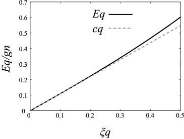
Figure 1: Quasiparticle energy spectrum for $g^{\prime}=0.5$ at the temperature $T=0.5T_{c}^{0}$.The solid line is the quasiparticle excitation spectrum $Eq$ in Eq. (46) and the dashed line is the sound-like energy spectrum $E_{q}=c\hbar q$ with $c=\sqrt{gn_{0}/m}$

In the HFB-Popov approximation, the thermodynamic potential is given by

$$\Omega=-\mu n_{0}V+\frac{1}{2}gn_{0}^{2}V+k_{\rm{B}}T\sum_{q}\ln\left(1-e^{-\beta E_{q}}\right)+\sum_{q}E_{q}v_{q}^{2}.$$ (50)

The pressure is the given by $P=-\Omega/V$. The entropy is given in terms of the quasiparticle excitation spectrum as

$$S=k_{\rm{B}}\sum_{q}\Big{\{}\big{[}1+f(E_{q})\big{]}\ln\big{[}1+f(E_{q})\big{]}-f(E_{q})\ln f(E_{q})\Big{\}}.$$ (51)

Using these thermodynamic quantities, one can calculate the sound velocities. The first and second sound velocities are given by

$$c^{2}_{12}=\frac{C_{s}^{2}+C_{2}^{2}}{2}\pm\sqrt{\left(\frac{C_{s}^{2}+C_{2}^{2}}{2}\right)^{2}-C_{T}^{2}C_{2}^{2}},$$ (52)

where $C_{s}^{2}=\left(\frac{\partial P}{\partial\rho}\right)_{\bar{s}}$, $C_{T}^{2}=\left(\frac{\partial P}{\partial\rho}\right)_{T}$, $C_{2}^{2}=\frac{\rho_{s0}}{\rho_{n0}}\frac{T\bar{s}^{2}_{0}}{\bar{C_{v}}}$. $C_{s}^{2}-C_{T}^{2}=\left(\frac{\partial s}{\partial\rho}\right)_{T}^{2}\frac{\rho^{2}T}{c_{v}}$.

Using the above results, we calculate the relative weights of first and second sound in $A(\mathbf{q},\omega)$ (see Eq. 6). We take the interaction parameter from the experiment of Ref. Meppelink et al. (2009), which reports the observation of second sound. In this experiment, total number of ²³Na atoms $N=1.7\times 10^{8}$, radial trap frequency $\omega_{\rm rad}/2\pi=95$Hz, and the aspect ratio $\omega_{\rm rad}/\omega_{\rm ax}\approx 65$. We estimate the interaction parameter for a uniform gas using the average density of the trapped gas, and obtain $g^{\prime}\sim 0.5~{}(na^{3}\sim 0.07)$. In Appendix B, we evaluate the characteristic collisional relaxation time and confirm that one is well in the hydrodynamic regime at intermediate temperature. In Fig. 2, we plot the the temperature dependence of the relative weights for $g^{\prime}=0.5$ and $g^{\prime}=1.02$. We see that there is no significant difference between the two results. In both cases, the first sound mode is dominant at low temperature, while the second sound is dominant at high temperature. This can be understood as follows. In the case of the superfluid velocity-velocity correlation, the external perturbation is directly coupled to the condensate motion. Therefore, the condensate mode should be always dominant in the spectral weight in the case of weakly-interacting Bose gas. At very low temperature (near $T=0$), the first sound mode is essentially the condensate collective mode and the second sound mode is the collective mode of quasiparticle excitations. With increasing temperature, there is a crossover between two modes, and the nature of the sound oscillations changes. At high temperatures, the first sound mostly involves the noncondensate oscillation, while the second sound mostly involves the condensate oscillation. In Appendix A, we compare the result with the self-consistent Hartree-Fock(HF) approximation. we see that the qualitative behaviors are well captured by the HF approximation. Moreover, we can explicitly see that in a weakly-interacting Bose gas, the single-particle spectrum is dominated by the condensate mode.

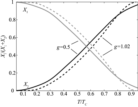
Figure 2: Temperature dependence of relative weights of first and second sound modes $X_{1}$ and $X_{2}$ for $g^{\prime}=0.5$ and $g^{\prime}=1.02$.

In Fig. 3, we compare the relative weights of first and second sound modes in both the single-particle spectral density $A({\bf q},\omega)$ and the dynamic structure factor $S({\bf q},\omega)$, where

$$S({\bf q},\omega) = [f(\omega)+1]\frac{q}{m}\left\{\frac{Z_{1}}{u_{1}}\left[\delta(\omega-u_{1}q)+\delta(\omega+u_{1}q)\right]+\frac{Z_{2}}{u_{2}}\left[\delta(\omega-u_{2}q)+\delta(\omega+u_{2}q)\right]\right\}$$ (53)

$$= \frac{q}{m}\left\{B_{1}(q)\left[\delta(\omega-u_{1}q)+\delta(\omega+u_{1}q)\right]+B_{2}(q)\left[\delta(\omega-u_{2}q)+\delta(\omega+u_{2}q)\right]\right\},$$

where

$$Z_{1}=\frac{u_{1}^{2}-v^{2}}{u_{1}-u^{2}},~{}~{}Z_{2}=1-Z_{1},$$ (54)

and

$$B_{1}(q)=[f(u_{1}q)+1]\frac{Z_{1}}{u_{1}},~{}~{}B_{2}(q)=[f(u_{2}q)+1]\frac{Z_{2}}{u_{2}}$$ (55)

We see that in $S({\bf q},\omega)$, the first sound mode is dominant at all temperatures. This is in sharp contrast with $A({\bf q},\omega)$, where the second sound mode is dominant near $T_{c}$.

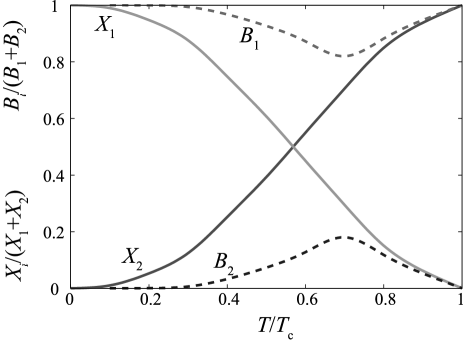
Figure 3: Comparison of the relative weights of first and second sound modes between $A({\bf q},\omega)$ and $S({\bf q},\omega)$.

IV Single-particle spectral density

We now discuss the single-particle spectral density in connection with the experiment such as the the photoemission spectroscopy Stewart et al. (2008). In a uniform gas, the photoemission current is related to spectral weight $I_{\rm sw}(\mathbf{q},\omega)\propto A(\mathbf{q},\omega)f(\omega)$ Törmä and Zoller (2000); Tsuchiya et al. (2010). In Fig. 4, we show $|A(\mathbf{q},\omega)f(\omega)|$ for $g^{\prime}=0.5$ at the temperature $T/T_{c}^{0}=0.5$ as a function of $q$ and $\omega$. In the plot, the energy delta function is replaced by a gaussian with a finite width: $\delta(\omega-c_{1}q)\to Ae^{a(\omega-c_{1}q)^{2}}$, where $a=1/4dq^{2}$ and $A=\sqrt{\frac{2\pi}{a}}$. Some appropriate value of the width parameter $d$ is used. In Fig. 4, the wavenumber $q$ and frequency $\omega$ are normalized in terms of the condensate healing lenght $\xi$ and the mean-field frequency $\omega_{0}=gn/\hbar$. For a parameter set we used, $\xi\approx 0.87\mu$m and $\omega_{0}\approx 2.7$kHz. The wavenumber and frequency are comparable to those in the recent experiment Stewart et al. (2008).

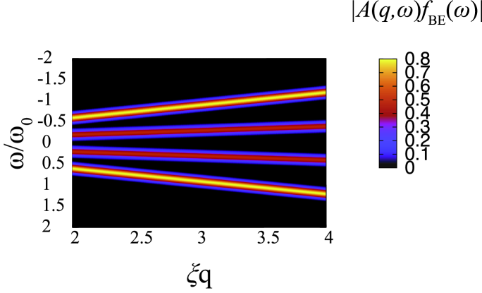
Figure 4: Plot of $A(\mathbf{q},\omega)$ as a function of $q$ and $\omega$ for $g^{\prime}=0.5~{}T=0.5T_{c}^{0}$.

For comparison, we also calculate $A(\mathbf{q},\omega)$ in the collisionless limit using the HFB-Popov approximation:

$$A^{\rm Popov}(\mathbf{q},\omega)=u^{2}_{q}\delta(\omega-E_{q})-v^{2}_{q}\delta(\omega+E_{q})$$ (56)

In Fig. 5, we plot this collisionless result for the same coupling and temperature $g^{\prime}=0.5,~{}T=0.5T_{\rm c}^{0}$. In the collisionless limit, there is only one sound mode. Moreover, it is clear from the expression (56) that the weights of $\omega=+E_{q}$ and $\omega=-E_{q}$ are different, since in general $u_{q}\neq v_{q}$. This is in contrast with the two-fluid hydrodynamic regime, where $\omega=+u_{1,2}q$ and $\omega=-u_{1,2}q$ have the same weights. In particular, for large $q$ one has $u_{q}\gg v_{q}$ and thus $A(\mathbf{q},\omega)$ only has the contribution from $\omega=+E_{q}$. In the opposite low-frequency limit, one has $u_{p}^{2}/v_{p}^{2}\to 1$.

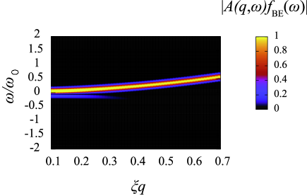
Figure 5: Plot of $A^{\rm Popov}(\mathbf{q},\omega)$ in the collisionless limit for $g^{\prime}=0.5,~{}T=0.5T_{\rm c}$.

V conclusion

In this paper, we have discussed single-particle spectral densities of first and second sound in superfluid Bose gases. In order to obtain the thermodynamic quantities available for calculating the single-particle spectral densities of the first and second sound modes, we use the HFB-Popov approximation. We showed that that both first and second sound mode can be observed by photoemission spectroscopy near $T\sim 0.5T_{\rm c}$. We showed that the first sound mode is dominant at low temperature, while the second sound is dominant at high temperature. With increasing temperature, there is a crossover between two modes, and the nature of the sound oscillations changes. We hope that our results will stimulate further experiment by photoemission spectroscopy in a superfluid Bose gas in the two-fluid hydrodynamic regime.

We have compared the relative weights of first and second sound modes in both the single-particle spectral density $A({\bf q},\omega)$ and the dynamic structure factor $S({\bf q},\omega)$. We showed that in $S({\bf q},\omega)$, the first sound mode is dominant at all temperatures. This is in sharp contrast with $A({\bf q},\omega)$, where the second sound mode is dominant near $T_{c}$.

For illustration, we also considered the self-consistent Hartree-Fock approximation. We showed that the qualitative behaviors are well captured by the HF approximation, but the quantitative details are quite different.

Finally, we showed thespectral weight $|A(\mathbf{q},\omega)f(\omega)|$ as a function of $q$ and $\omega$. We found that both first and second sound mode can be observed by photoemission spectroscopy.

VI ACKNOWLEDGMENTS

We thank S. Tsuchiya for valuable comments. This research was supported by Academic Frontier Project (2005) of MEXT. E. A. is supported by a Grant-in-Aid from JSPS.

Appendix A Self-consistent Hartree-Fock approximation and the ZNG hydrodynamics

For illustration, we consider the self-consistent Hartree-Fock approximation. In this approximation, the noncondensate density is given by

$$\tilde{n}=\frac{1}{\Lambda^{3}}g_{3/2}(z),$$ (57)

where $\Lambda$ is the thermal de Broglie wavelength defined by

$$\Lambda=\left(\frac{2\pi\hbar^{2}}{mk_{\rm B}T}\right)^{1/2},$$ (58)

and the fugacity $z$ is given by

$$z=\exp(-\beta gn_{c}),$$ (59)

where $n_{c}=n-\tilde{n}$. The pressure is given by

$$P=\tilde{P}+\frac{1}{2}g(n^{2}+2n\tilde{n}-\tilde{n}^{2})=\tilde{P}+\frac{1}{2}g(n_{c}^{2}+4\tilde{n}n_{c}+2\tilde{n}^{2}),$$ (60)

where $\tilde{P}$ is the kinetic pressure given by

$$\tilde{P}=\frac{k_{\rm B}T}{\Lambda^{3}}g_{5/2}(z)$$ (61)

The entropy is given by

$$S=\frac{1}{T}\left(\frac{5}{2}\tilde{P}+g\tilde{n}n_{c}\right)$$ (62)

We can then calculate the various thermodynamic derivatives used in the single-particle spectral function.

Alternatively, one can use the linearized ZNG hydrodynamic equations Griffin et al. (2009); Zaremba et al. (1999), which are based on the self-consistent HF approximation, to derive the superfluid velocity-velocity correlation function. The coupled equations for the condensate and noncondensate variables are given by

$$\frac{\partial\delta\tilde{n}}{\partial t} = -\tilde{n}_{0}({\nabla}\cdot\delta{\bf v}_{n})+\delta\Gamma_{12},$$ (63)

$$m\tilde{n}_{0}\frac{\partial\delta{\bf v}_{n}}{\partial t} = -{\nabla}\delta\tilde{P}-2g\tilde{n}_{0}{\nabla}(\delta\tilde{n}+\delta n_{c}),$$ (64)

$$\frac{\partial\delta\tilde{P}}{\partial t} = -\frac{5}{3}\tilde{P}_{0}({\nabla}\cdot\delta{\bf v}_{n})\cdot{\nabla}\tilde{P}_{0}+\frac{2}{3}(\mu_{c0}-U_{0})\delta\Gamma_{12}\,,$$ (65)

$$\frac{\partial\delta n_{c}}{\partial t} = -n_{c0}({\nabla}\cdot\delta{\bf v}_{c})-\delta\Gamma_{12},$$ (66)

$$m\frac{\partial\delta{\bf v}_{c}}{\partial t} = -{\nabla}\delta\mu_{c},$$ (67)

where

$$\delta\mu_{c}({\bf r},t)=g\delta n_{c}({\bf r},t)+2g\delta\tilde{n}({\bf r},t)\,.$$ (68)

The expression for $\delta\Gamma_{12}$ is given by

$$\delta\Gamma_{12}[\tilde{f}]=-\frac{\beta_{0}n_{c0}}{\tau_{12}}\delta\mu_{\rm diff},~{}~{}~{}\mu_{\rm diff}\equiv\tilde{\mu}-\mu_{c}.$$ (69)

In order to calculate the superfluid velocity-velocity correlation function, we add a time-dependent external current $\delta{\bf j}_{\rm ex}({\bf r},t)$ to the equation of motion for $\delta n_{c}$ given in (66). That is, we use

$$\frac{\partial\delta n_{c}}{\partial t}=-n_{c0}({\nabla}\cdot\delta{\bf v}_{c})-\nabla\cdot\delta{\bf j}_{\rm ex}-\delta\Gamma_{12},\\$$ (70)

To solve the hydrodynamic equations, we introduce velocity potentials according to $\delta{\bf v}_{c}\equiv{\nabla}\phi_{c}$ and $\delta{\bf v}_{n}\equiv{\nabla}\phi_{n}$. In terms of these new variables, the equations for the condensate and the equations for the noncondensate can be combined to give

$$m\frac{\partial^{2}\phi_{c}}{\partial t^{2}} = gn_{c0}\nabla^{2}\phi_{c}+2g\tilde{n}_{0}\nabla^{2}\phi_{n}+\frac{\sigma_{H}}{\tau_{\mu}}\delta\mu_{\rm diff}+g\nabla\cdot\delta{\bf j}_{\rm ex},$$ (71)

$$m\frac{\partial^{2}\phi_{n}}{\partial t^{2}} = \left(\frac{5\tilde{P}_{0}}{3\tilde{n}_{0}}+2g\tilde{n}_{0}\right)\nabla^{2}\phi_{n}+2gn_{c0}\nabla^{2}\phi_{c}-\frac{2\sigma_{H}}{3\tau_{\mu}}\frac{n_{c0}}{\tilde{n}_{0}}\delta\mu_{\rm diff}+2g\nabla\cdot\delta{\bf j}_{\rm ex}.$$ (72)

Here $\delta\Gamma_{12}$ has been expressed in terms of $\delta\mu_{\rm diff}$ using (69). The equation of motion for $\delta\mu_{\rm diff}$ is given by (15.71)

$$\frac{\partial\delta\mu_{\rm diff}}{\partial t}=\frac{2}{3}gn_{c0}\nabla^{2}\phi_{n}-gn_{c0}\nabla^{2}\phi_{c}-g\nabla\cdot\delta{\bf j}_{\rm ex}-\frac{\delta\mu_{\rm diff}}{\tau_{\mu}}.$$ (73)

We now consider an external current which excites modes of frequency $\omega$ and wavevector ${\bf q}$

$$\delta{\bf j}_{\rm ex}({\bf r},t)=\delta{\bf j}_{\rm ex}({\bf q},\omega)e^{i({\bf q}\cdot{\bf r}-\omega t)},$$ (74)

and look for the plane-wave solutions $\phi_{c,n}({\bf r},t)=\phi_{c,n,{\bf q},\omega}e^{i({\bf q}\cdot{\bf r}-\omega t)}.$ In this case, (73) reduces to

$$\delta\mu_{\rm diff}=\frac{\tau_{\mu}}{1-i\omega\tau_{\mu}}\left[gn_{c0}\left(\phi_{c}-\frac{2}{3}\phi_{n}\right)q^{2}-ig{\bf q}\cdot\delta{\bf j}_{\rm ex}\right].$$ (75)

Substituting this result into (71) and (72), we are left with two coupled equations for the superfluid and normal fluid velocity potentials:

$$m\omega^{2}\phi_{c,{\bf q},\omega} = gn_{c0}\Bigg{(}1-\frac{\sigma_{H}}{1-i\omega\tau_{\mu}}\Bigg{)}q^{2}\phi_{c,{\bf q},\omega}+2g\tilde{n}_{0}\left[1+\frac{\sigma_{H}}{3(1-i\omega\tau_{\mu})}\frac{n_{c0}}{\tilde{n}_{0}}\right]q^{2}\phi_{n,{\bf q},\omega}$$ (76)

$$-ig\Bigg{(}1-\frac{\sigma_{H}}{1-i\omega\tau_{\mu}}\Bigg{)}{\bf q}\cdot\delta{\bf j}_{\rm ex}({\bf q},\omega),$$

and

$$m\omega^{2}\phi_{n,{\bf q},\omega}=\Bigg{\{}\frac{5\tilde{P}_{0}}{3\tilde{n}_{0}} + 2g\tilde{n}_{0}\left[1-\frac{2\sigma_{H}}{9(1-i\omega\tau_{\mu})}\frac{n_{c0}^{2}}{\tilde{n}_{0}^{2}}\right]\Bigg{\}}q^{2}\phi_{n,{\bf q},\omega}$$ (77)

$$+ 2gn_{c0}\left[1+\frac{\sigma_{H}}{3(1-i\omega\tau_{\mu})}\frac{n_{c0}}{\tilde{n}_{0}}\right]q^{2}\phi_{c,{\bf q},\omega}$$

$$- i2g\left[1+\frac{\sigma_{H}}{3(1-i\omega\tau_{\mu})}\frac{n_{c0}}{\tilde{n}_{0}}\right]{\bf q}\cdot\delta{\bf j}_{\rm ex}({\bf q},\omega).$$

Taking the limit $\omega\tau_{\mu}\to 0$ of these coupled equations, we obtain

$$m\omega^{2}\phi_{c,{\bf q},\omega} = gn_{c0}(1-\sigma_{H})q^{2}\phi_{c,{\bf q},\omega}+2g\tilde{n}_{0}\left(1+\frac{\sigma_{H}n_{c0}}{3\tilde{n}_{0}}\right)q^{2}\phi_{n,{\bf q},\omega}$$ (78)

$$-ig(1-\sigma_{H}){\bf q}\cdot\delta{\bf j}_{\rm ex}({\bf q},\omega),$$

$$m\omega^{2}\phi_{n,{\bf q},\omega} = \Bigg{[}\frac{5\tilde{P}_{0}}{3\tilde{n}_{0}}+2g\tilde{n}_{0}\left(1-\frac{2\sigma_{H}n_{c0}^{2}}{9\tilde{n}_{0}^{2}}\right)\Bigg{]}q^{2}\phi_{n,{\bf q},\omega}$$ (79)

$${}{}{}+2gn_{c0}\left(1+\frac{\sigma_{H}n_{c0}}{3\tilde{n}_{0}}\right)q^{2}\phi_{c,{\bf q},\omega}-i2g\left(1+\frac{\sigma_{H}n_{c0}}{3\tilde{n}_{0}}\right){\bf q}\cdot\delta{\bf j}_{\rm ex}({\bf q},\omega).$$

It is useful to rewrite (78) and (79) in a simple matrix form as

$$\left(\begin{array}[]{cc}\omega^{2}-v_{2}^{2}q^{2}&-v_{21}^{2}q^{2}\\ -v_{12}^{2}q^{2}&\omega^{2}-v_{1}^{2}q^{2}\\ \end{array}\right)\left(\begin{array}[]{c}\phi_{c,{\bf q},\omega}\\ \phi_{n,{\bf q},\omega}\end{array}\right)=-i\frac{{\bf q}\cdot\delta{\bf j}_{\rm ex}({\bf q},\omega)}{n_{c0}}\left(\begin{array}[]{c}v_{2}^{2}\\ v_{12}^{2}\end{array}\right),$$ (80)

where we have introduced new velocities

$$v_{2}^{2} = \frac{gn_{c0}}{m}(1-\sigma_{H}),~{}~{}v_{21}^{2}=\frac{2g\tilde{n}_{0}}{m}\left(1+\frac{\sigma_{H}n_{c0}}{3\tilde{n}_{0}}\right),$$

$$v_{12}^{2} = \frac{2gn_{c0}}{m}\left(1+\frac{\sigma_{H}n_{c0}}{3\tilde{n}_{0}}\right),~{}~{}v_{1}^{2}=\frac{5\tilde{P}_{0}}{3m\tilde{n}_{0}}+\frac{2g\tilde{n}_{0}}{m}\left(1-\frac{2\sigma_{H}n_{c0}^{2}}{9\tilde{n}_{0}^{2}}\right).$$ (81)

We note that these new velocities are related to the first and second sound velocities $u_{1}$ and $u_{2}$ through

$$u_{1}^{2}+u_{2}^{2}=v_{1}^{2}+v_{2}^{2},~{}~{}u_{1}^{2}u_{2}^{2}=v_{1}^{2}v_{2}^{2}-v_{12}^{2}v_{21}^{2}.$$ (82)

Solving (80), we obtain

$$\left(\begin{array}[]{c}\phi_{c,{\bf q},\omega}\\ \phi_{n,{\bf q},\omega}\end{array}\right)=-i\frac{{\bf q}\cdot\delta{\bf j}_{\rm ex}({\bf q},\omega)}{n_{c0}}\frac{1}{(\omega^{2}-u_{1}^{2}q^{2})(\omega^{2}-u_{2}^{2}q^{2})}\left(\begin{array}[]{cc}\omega^{2}-v_{1}^{2}q^{2}&v_{21}^{2}q^{2}\\ v_{12}^{2}q^{2}&\omega^{2}-v_{2}^{2}q^{2}\\ \end{array}\right)\left(\begin{array}[]{c}v_{2}^{2}\\ v_{12}^{2}\end{array}\right).$$ (83)

We thus obtain

$$\phi_{c,{\bf q},\omega}=-i\frac{{\bf q}\cdot\delta{\bf j}_{\rm ex}}{n_{c0}}\frac{v_{2}^{2}\omega^{2}-(v_{1}^{2}v_{2}^{2}-v_{12}^{2}v_{21}^{2})q^{2}}{(\omega^{2}-u_{1}^{2}q^{2})(\omega^{2}-u_{2}^{2}q^{2})}.$$ (84)

From (84), we obtain the superfluid velocity $\delta{\bf v}_{c}({\bf r},t)=\delta{\bf v}_{c,{\bf q},\omega}e^{i({\bf q}\cdot{\bf r}-\omega t)}$, where

$$\delta{\bf v}_{c,{\bf q},\omega}=i{\bf q}\phi_{c,{\bf q},\omega}=\frac{{\bf q}({\bf q}\cdot\delta{\bf j}_{\rm ex})}{n_{c0}}\frac{v_{2}^{2}\omega^{2}-(v_{1}^{2}v_{2}^{2}-v_{12}^{2}v_{21}^{2})q^{2}}{(\omega^{2}-u_{1}^{2}q^{2})(\omega^{2}-u_{2}^{2}q^{2})}.$$ (85)

This result can be written in terms of the superfluid velocity-velocity correlation function, defined as

$$\delta v_{c\mu,{\bf q},\omega}=m\sum_{\nu}\chi_{v_{s}v_{s}}^{\mu\nu}({\bf q},\omega)\delta j_{{\bf q},\omega,\nu}.$$ (86)

Comparing (86) with (85), we find

$$\chi_{v_{s}v_{s}}^{\mu\nu}({\bf q},\omega)=\frac{q_{\mu}q_{\nu}}{mn_{c0}}\frac{v_{2}^{2}\omega^{2}-u_{1}^{2}u_{2}^{2}q^{2}}{(\omega^{2}-u_{1}^{2}q^{2})(\omega^{2}-u_{2}^{2}q^{2})}.$$ (87)

The longitudinal part of the superfluid velocity-velocity correlation function is given by

$$\chi_{v_{s}v_{s}}({\bf q},\omega)=\frac{q^{2}}{mn_{\rm c0}}\frac{v_{2}^{2}\omega^{2}-u_{1}^{2}u_{2}^{2}q^{2}}{(\omega^{2}-u_{1}^{2}q^{2})(\omega^{2}-u_{2}^{2}q^{2})}.$$ (88)

Comparing this result with the general expression (1), we see that in the HF approximation one has $\rho_{s}\lambda_{v_{s}v_{s}}=v_{2}^{2}$ with $\rho_{s}=mn_{\rm c0}$. The single-particle Green’s function is given by

$$G({\bf q},\omega)=\frac{n_{\rm c0}m^{2}}{q^{2}}\chi_{v_{s}v_{s}}({\bf q},\omega)=\frac{m(v_{2}^{2}\omega^{2}-u_{1}^{2}u_{2}^{2}q^{2})}{(\omega^{2}-u_{1}^{2}q^{2})(\omega^{2}-u_{2}^{2}q^{2})}.$$ (89)

This Green’s function can be expressed in terms of the single-particle spectral density through the relation (4). In this case, we have

$$A({\bf q},\omega) = 2\pi m~{}{\rm sgn}(\omega)\left[\frac{u_{1}^{2}(v_{2}^{2}-u_{2}^{2})}{u_{1}^{2}-u_{2}^{2}}\delta(\omega^{2}-u_{1}^{2}q^{2})+\frac{u_{2}^{2}(u_{1}^{2}-v_{2}^{2})}{u_{1}^{2}-u_{2}^{2}}\delta(\omega^{2}-u_{2}^{2}q^{2})\right]$$ (90)

$$= \frac{\pi m}{q}\Bigg{\{}X_{1}\left[\delta(\omega-u_{1}q)-\delta(\omega+u_{1}q)\right]+X_{2}\left[\delta(\omega-u_{2}q)-\delta(\omega+u_{2}q)\right]\Bigg{\}},$$

where

$$X_{1}=\frac{u_{1}(v_{2}^{2}-u_{2}^{2})}{u_{1}^{2}-u_{2}^{2}},~{}~{}~{}X_{2}=\frac{u_{2}(u_{1}^{2}-v_{2}^{2})}{u_{1}^{2}-u_{2}^{2}}.$$ (91)

The above expressions should be compared with the general expressions (6). If we use the expression for $u_{2}$ to order $g^{2}$ given by (15.86), one has

$$v_{2}^{2}=u_{2}^{2}+\Delta v^{2},~{}~{}~{}\Delta v^{2}\equiv\frac{gn_{c0}}{m}\frac{3m\tilde{n}_{0}}{5\tilde{P}_{0}}\frac{4g\tilde{n}_{0}}{m},$$ (92)

and the weights $X_{1}$ and $X_{2}$ can be approximated as

$$X_{1}\approx\frac{u_{1}\Delta v^{2}}{u_{1}^{2}-u_{2}^{2}},~{}~{}X_{2}\approx\left(1-\frac{\Delta v^{2}}{u_{1}^{2}-u_{2}^{2}}\right)u_{2}$$ (93)

We find from (93) that the contribution at the second sound mode $\omega^{2}=u_{2}^{2}q^{2}$ is larger than the contribution at the first sound mode $\omega^{2}=u_{1}^{2}q^{2}$.

Figure 6 compares the sound velocities calculated by the HF approximation with those calculated by the HFB-Popov approximation. Figure 7 compares $X_{1}$ and $X_{2}$ calculated by the HF approximation with those calculated by the HFB-Popov approximation. We see that the qualitative behaviors are well captured by the HF approximation, but the quantitative details are different.

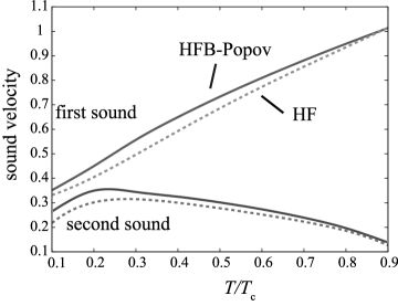
Figure 6: Sound velocities of the first sound and second sound modes. dash Lines show the results from the self-consistent HF approximation, solid lines are the results from the HFB-Popov approximation.$g^{\prime}=0.5$.

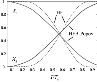
Figure 7: The temperature dependence of the amplitudes $X_{1},X_{2}$. dash Lines show the results from the self-consistent HF approximation. Solid lines are results from the HFB-Popov approximation. $g^{\prime}=0.5$.

Appendix B Validity of Hydrodynamics

Here we discuss the validity of using Landau’s two-fluid hydrodynamics in the experiment of Ref. Meppelink et al. (2009). In Fig. 8, we plot the temperature dependence of the collisional relaxation time $\tau_{\mu}$ defined in Ref. Zaremba et al. (1999); Nikuni and Griffin (2001). This relaxation time $\tau_{\mu}$ describes the rate of equilibration of the condensate and noncondensate chemical potential. The condition for the hydrodynamic regime is described by $\omega\tau_{\mu}\leq 1$ where $\omega$ is the frequency of the collective mode. We see that the collective mode of the frequency $\omega\sim gn/\hbar$ is well within the hydrodynamic regime in the intermediate temperature region $T\sim 0.5T_{\rm c}$.

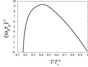
Figure 8: Temperature dependence of the relaxation time $\tau_{\mu}$. $g^{\prime}=0.5$.

References

Griffin et al. (2009)
A. Griffin,
T. Nikun, and
E. Zaremba,
Bose-Condensed Gases at Finite Temperatures
(UNIVERSITY PRESS CAMBRIDGE, 2009).
Landau (1941)
L. D. Landau,
J. Phys. (USSR) 5,
71 (1941).
Heiselberg (2006)
H. Heiselberg,
Phys. Rev. A 73,
013607 (2006).
Capuzzi et al. (2006)
P. Capuzzi,
P. Vignolo,
F. Federici, and
M. P. Tosi,
Phys. Rev. A 73,
021603(R) (2006).
Joseph et al. (2007)
J. Joseph,
B. Clancy,
L. Luo,
J. Kinast,
A. Turlapov, and
J. E. Thomas,
Phys. Rev. Lett. 98,
170401 (2007).
Meppelink et al. (2009)
R. Meppelink,
S. B. Koller,
and P. van der
Straten, Phys. Rev. A 80,
043605 (2009).
Hu et al. (2010)
H. Hu,
E. Taylor,
X.-J. Liu,
S. Stringari,
and A. Griffin,
New J. Phys. 12,
043040 (2010).
Kinast et al. (2004)
J. Kinast,
S. L. Hemmer,
M. E. Gehm,
A. Turlapov, and
J. E. Thomas,
Phys. Rev. Lett. 92,
150402 (2004).
Bartenstein et al. (2004)
M. Bartenstein,
A. Altmeyer,
S. Riedl,
S. Jochim,
C. Chin,
J. H. Denschlag,
and R. Grimm,
Phys. Rev. Lett 92,
203201 (2004).
Massignan et al. (2005)
P. Massignan,
G. M. Bruun, and
H. Smith,
Phys. Rev. A 71,
033607 (2005).
Hohenberg and Martin (1965)
P. C. Hohenberg
and P. C.
Martin, Ann. Phys. (NY)
34, 291 (1965).
Luxat and Griffin (2002)
D. L. Luxat and
A. Griffin,
Phys. Rev. A 65,
043618 (2002).
Stewart et al. (2008)
J. T. Stewart,
J. P. Gaebler,
and D. S. Jin,
Nature 454,
744 (2008).
Griffin (1996)
A. Griffin,
Phys. Rev. B 53,
9341 (1996).
Törmä and Zoller (2000)
P. Törmä
and P. Zoller,
Phys. Rev. Lett 85,
487 (2000).
Tsuchiya et al. (2010)
S. Tsuchiya,
R. Watanabe, and
Y. Ohashi,
Phys. Rev. A 82,
033629 (2010).
Kadanoff and Martin (1963)
L. P. Kadanoff and
P. C. Martin,
Ann. Phys. (NY) 24,
419 (1963).
Zaremba et al. (1999)
E. Zaremba,
T. Nikuni, and
A. Griffin,
J. Low Temp. Phys. 116,
277 (1999).
Nikuni and Griffin (2001)
T. Nikuni and
A. Griffin,
Phys. Rev. A 65,
011601 (2001).