Bell inequality test with entanglement between an atom and a coherent state in a cavity

Abstract

We study Bell inequality tests with entanglement between a coherent-state field in a cavity and a two-level atom. In order to detect the cavity field for such a test, photon on/off measurements and photon number parity measurements, respectively, are investigated. When photon on/off measurements are used, at least 50% of detection efficiency is required to demonstrate violation of the Bell inequality. Photon number parity measurements for the cavity field can be effectively performed using ancillary atoms and an atomic detector, which leads to large degrees of Bell violations up to Cirel’son’s bound. We also analyze decoherence effects in both field and atomic modes and discuss conditions required to perform a Bell inequality test free from the locality loophole.

I Introduction

Einstein, Podolsky, and Rosen (EPR) presented an argument known as the EPR paradox Einstein1935 , which triggered the debate on quantum mechanics versus local realism. Bell’s theorem Bell1964 enables one to perform experiments in which failure of local realism is demonstrated by the violation of Bell’s inequality. Various versions of Bell’s inequality have been developed including Clauser, Horne, Shimony and Holt (CHSH)’s one Clauser1969 , and substantial amount of experimental efforts have been devoted to the successful demonstration of violation of Bell’s inequality. So far, many experiments have been performed to show violation of Bell-type inequalities, and most physicists now seem to believe that local realism can be violated.

On the other hand, all the experiments performed to date are subject to some loopholes, so that the experimental data can still be explained somehow based on a classical (often impellent) argument. Experiments using optical fields Freedman1972 ; Aspect1981 ; Tittel1998 ; Weihs1998 typically suffer from the “detection loophole” Pearle1970 , and recent experiments using atomic states Rowe2001 ; Matsukevich2008 with the maximum separation of $\sim 1$ m Matsukevich2008 , suffer from the “locality loophole” Bell1981 . While most of Bell inequality tests have been performed using entangled optical fields Freedman1972 ; Aspect1981 ; Tittel1998 ; Weihs1998 , it is an interesting possibility to explore Bell inequality tests using atom-field entanglement MSKim2000 ; Milman2005 ; Simon2003 ; Volz2006 ; Brunner2007 , particularly for a loophole-free test. In fact, there exist theoretical proposals for a loophole-free Bell inequality test using hybrid entanglement between atoms and photons Simon2003 ; San2011 ; Spa2011 and relevant experimental efforts Moehring2004 ; Volz2006 ; Matsukevich2008 have been reported.

In this paper, we study Bell inequality tests with an entangled state of a two-level atom and a coherent-state field. When the amplitude of the coherent state is large enough, such an entangled state is often called a “Schrödinger cat state” (e.g. in Ref. Wodkiewicz2000 ) as an analogy of Schrödinger’s paradox where entanglement between a microscopic atom and a classical object is illustrated Schrodinger1935 . Entanglement between atoms and coherent states has been experimentally demonstrated using cavities Brune1996 ; Guerlin2007 ; Deleglise2008 .

In our study, photon on/off measurements and photon number parity measurements, respectively, are employed in order to detect the cavity field. We find that when photon on/off measurements are used, at least 50% of detection efficiency is required to demonstrate violation of the Bell-CHSH inequality. One may effectively perform photon number parity measurements for the cavity field using ancillary probe atoms and an atomic detector so that nearly the maximum violation of the Bell-CHSH inequality can be achieved.

The remainder of this paper is organized as follows. In Sec. II, we briefly discuss the atom-field entanglement under consideration and review basic elements of Bell inequality tests in our framework. We then investigate the Bell-CHSH inequality with photon on/off measurements and parity measurements, respectively, in Sec. III. Sec. IV is devoted to the investigation of the Bell-CHSH inequality test using indirect measurements within a ‘circular Rydberg atom’-‘microwave cavity’ system. In Sec. V, we analyze decoherence effects in both field and atomic modes. This analysis enables us to provide quantitative information on the requirements to perform a loophole-free Bell test. We conclude with final remarks in Sec. VI.

II Basic elements for Bell inequality tests

We are interested in testing the Bell-CHSH inequality with an atom-field entangled state:

$$|\Psi\rangle_{AC}=\frac{1}{\sqrt{2}}\left(|e\rangle_{A}|\alpha\rangle_{C}+|g\rangle_{A}|-\alpha\rangle_{C}\right),$$ (1)

where $|e\rangle_{A}$ ($|g\rangle_{A}$) is the excited (ground) state for the atomic mode $A$, and $|\pm\alpha\rangle_{C}$ are coherent states of amplitudes $\pm\alpha$ for the field mode $C$. States (1) for reasonably large values of $\alpha$ are considered entanglement between a microscopic system and a classical system Wodkiewicz2000 ; Jeong2006Sep ; Martini2008Jun ; Spagnolo2010Nov . There have been studies on Bell inequality tests with this type of entangled state Wodkiewicz2000 , and similar states such as entanglement between an atom and a single photon MSKim2000 ; Milman2005 ; Simon2003 ; Volz2006 and entanglement between coherent states Munro2000 ; Wilson2002 ; Jeong2003 ; JeongSole2008 ; Jeong2009 ; Jeong2006Sep ; JeongAn2006 ; Stobinska2007 ; Gerry2009 ; LeeJeong2009 . Experimental demonstration of state (1) has been performed using a system composed of a circular Rydberg atom and a microwave cavity field Brune1996 ; Guerlin2007 ; Deleglise2008 .

In order to test a Bell type inequality, a bipartite entangled state should be shared by two separate parties. After sharing the entangled state, each of the two parties may locally perform appropriate unitary operations and dichotomic measurements. Violation of the Bell-CHSH inequality can be obtained by choosing certain values for the parameters of the unitary operations. The correlation function is defined as the expectation value of the joint measurement

$$E(\zeta,\beta)=\langle\hat{E}_{A}(\zeta)\otimes\hat{E}_{C}(\beta)\rangle,$$ (2)

where $\hat{E}_{A}(\zeta)=\hat{U}_{A}^{{\dagger}}(\zeta)\hat{\Gamma}_{A}\hat{U}_{A}(\zeta)$ is a dichotomic measurement $\hat{\Gamma}_{A}$ combined with unitary operation $\hat{U}_{A}(\zeta)$ parameterized by $\zeta$, and $\hat{E}_{C}(\beta)$ can be defined accordingly. The Bell function $\cal{B}$ is then defined as

$$\begin{split}{\cal B}=\left|E(\zeta,\beta)+E(\zeta^{\prime},\beta)+E(\zeta,\beta^{\prime})-E(\zeta^{\prime},\beta^{\prime})\right|,\end{split}$$ (3)

which should obey the inequality forced by local realism, i.e., ${\cal B}\leq 2$. The maximum bound for the absolute value of the Bell function is $2\sqrt{2}$, known as Cirel’son’s bound Cirelson1980 .

An atomic dichotomic measurement can be represented by a 2 by 2 matrix

$$\hat{\Gamma}=\left({\begin{array}[]{*{20}c}1&0\\ 0&{-1}\\ \end{array}}\right)$$ (4)

where we choose the basis as {$|e\rangle$, $|g\rangle$}. We define the displaced dichotomic measurement $\hat{\Gamma}(\zeta)$ with the atomic displacement operator $\hat{D}(\zeta)$ as

$$\hat{\Gamma}(\zeta)=\hat{D}(\zeta){\hat{\Gamma}}{{\hat{D}}}^{{\dagger}}(\zeta)$$ (5)

with

$$\begin{split}&\hat{D}(\zeta)=\exp{[{\zeta\hat{\sigma}_{+}-\zeta^{*}\hat{\sigma}_{-}}]}=\left(\begin{array}[]{cc}\cos{\left|\zeta\right|}&\frac{\zeta}{\left|\zeta\right|}\sin{\left|\zeta\right|}\\ -\frac{\zeta^{*}}{\left|\zeta\right|}\sin{\left|\zeta\right|}&\cos{\left|\zeta\right|},\end{array}\right),\\ &\zeta(\theta,~{}\phi)=-\frac{\theta}{2}e^{-i\phi},\end{split}$$ (6)

and $0\leq\theta\leq\pi$ and $0\leq\phi\leq 2\pi$, where $\hat{\sigma}_{\pm}$ are the standard ladder operators in the $2$-dimensional Hilbert space. We note that $\hat{D}(\zeta)$ corresponds to a single qubit rotation for an atomic qubit and it can be achieved by applying a Ramsey pulse to the atom Haroche2006 . We consider measurement $\hat{\Gamma}(\zeta)$ for the atomic mode $A$ throughout the paper, while some different measurement schemes are considered for the field mode $C$.

III Bell-CHSH inequality tests with atom-field entanglement

III.1 On/off measurement for field mode

We first investigate the Bell-CHSH inequality with photon on/off measurements and the displacement operator for the cavity field mode. The displaced on/off measurement for the field $C$ is

$$\begin{split}\hat{\cal{O}}_{C}(\beta)&=\hat{\cal D}_{C}(\beta)\Big{(}\sum_{n=1}^{\infty}|n\rangle\langle n|-|0\rangle\langle 0|\Big{)}\hat{\cal D}^{{\dagger}}_{C}(\beta),\\ \end{split}$$ (7)

where $\hat{\cal D}_{C}(\beta)=\exp[{\beta}\hat{a}_{C}^{\dagger}-{\beta}^{*}\hat{a}_{C}]$ is the displacement operator with the field annihilation (creation) operator $\hat{a}_{C}$ ($\hat{a}_{C}^{\dagger}$) and $\beta$ as the displacement parameter for field $C$.

We model a photodetector with efficiency $\eta$ by a perfect photodetector together with a beam splitter of transmissivity $\sqrt{\eta}$ in front of it Yuen1980 . The signal field $C$ is mixed with the vacuum state $\left|0\right\rangle_{v}$ at a beam splitter. The beam splitter operator between modes $C$ and $v$ is $\hat{B}_{Cv}=\exp[(\cos^{-1}{\sqrt{\eta}})(\hat{a}_{C}^{\dagger}\hat{a}_{v}-\hat{a}_{C}\hat{a}_{v}^{\dagger})/2]$ Campos1989 , where $\hat{a}_{v}$ ($\hat{a}_{v}^{\dagger}$) is the field annihilation (creation) operator for the ancilla mode $v$. After passing through the beam splitter, the atom-field entangled state $|\Psi\rangle_{AC}$ is changed to a mixed state as

$$\begin{split}\rho^{\eta}_{AC}=&{\rm Tr}_{v}\left[\hat{B}_{Cv}\Big{(}|\Psi\rangle\langle\Psi|\Big{)}_{AC}\otimes\Big{(}|0\rangle\langle 0|\Big{)}_{v}\hat{B}_{Cv}^{{\dagger}}\right]\\ =&\frac{1}{2}\Big{\{}|e\rangle\langle e|\otimes|\sqrt{\eta}\alpha\rangle\langle\sqrt{\eta}\alpha|+|g\rangle\langle g|\otimes|-\sqrt{\eta}\alpha\rangle\langle-\sqrt{\eta}\alpha|\\ &~{}~{}~{}+e^{-2(1-\eta)\left|\alpha\right|^{2}}|e\rangle\langle g|\otimes|\sqrt{\eta}\alpha\rangle\langle-\sqrt{\eta}\alpha|\\ &~{}~{}~{}+e^{-2(1-\eta)\left|\alpha\right|^{2}}|g\rangle\langle e|\otimes|-\sqrt{\eta}\alpha\rangle\langle\sqrt{\eta}\alpha|\Big{\}}_{AC}.\end{split}$$ (8)

The correlation function with the photon detection efficiency $\eta$ is the expectation value of $\hat{{\Gamma}}_{A}(\zeta)\otimes\hat{\cal{O}}_{C}(\beta)$ for state (8) as

$$E_{\cal{O}}(\zeta,\beta;\eta)= {\rm Tr}\Big{[}\rho^{\eta}_{AC}\hat{{\Gamma}}_{A}(\zeta)\otimes\hat{\cal{O}}_{C}(\beta)\Big{]}$$ (9)

$$= -e^{-|\beta|^{2}-|\alpha|^{2}\eta-2|\alpha||\beta|\sqrt{\eta}\cos\Phi}\cos\frac{\theta}{2}$$

$$+e^{-|\beta|^{2}-|\alpha|^{2}\eta+2|\alpha||\beta|\sqrt{\eta}\cos\Phi}\cos\frac{\theta}{2}$$

$$+e^{-2|\alpha|^{2}}\cos\phi\sin\frac{\theta}{2}$$

$$-2e^{-2|\alpha|^{2}-|\beta|^{2}+|\alpha|^{2}\eta}\cos\left(\phi-2|\alpha||\beta|\sqrt{\eta}\sin\Phi\right)\sin\frac{\theta}{2},$$

where $\alpha=|\alpha|e^{i\Phi_{\alpha}}$, $\beta=|\beta|e^{i\Phi_{\beta}}$, and $\Phi=\Phi_{\beta}-\Phi_{\alpha}$ with real phase parameters $\Phi_{\alpha}$ and $\Phi_{\beta}$. The Bell function is immediately obtained using Eqs. (3) and (LABEL:eq:qtypecorrelation).

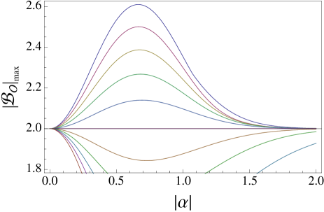
Figure 1: (Color online) Numerically optimized values of Bell functions $\cal{B}_{\cal{O}}$ with displaced on/off measurements against amplitude $\alpha$ of state (1). The detection efficiency ranges in value from $\eta=0$ (lower curve) to $\eta=1$ (upper curve), with intervals of 0.1 shown by the family of curves. The horizontal line corresponds to the case of $\eta=0.5$, which coincides with the classical limit of the Bell-CHSH inequality.

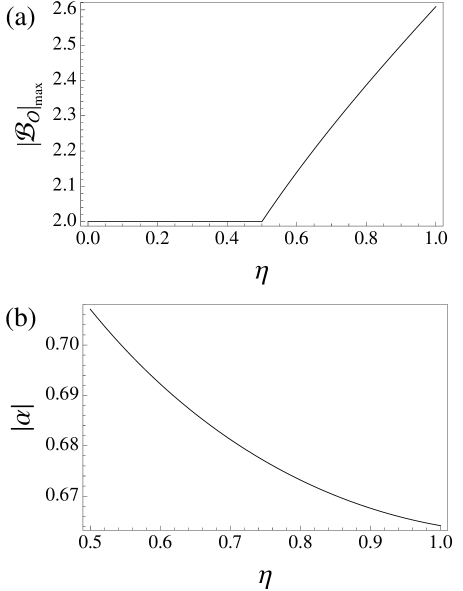
Figure 2: (a) Numerically optimized values of Bell function $\cal{B}_{\cal{O}}$ with displaced on/off measurements against detection efficiency $\eta$. The local realistic bound, 2, is violated for $\eta\geq 0.5$. (b) Plot of optimizing values of $|\alpha|$ with respect to $\eta$.

Using the method of steepest descent Pres1988 , we numerically find optimized values, $|{\cal B}_{\cal{O}}|_{\rm max}$, i.e., absolute values of the Bell function maximized over variables $\zeta$, $\zeta^{\prime}$, $\beta$ and $\beta^{\prime}$. We plot the results against amplitude $|\alpha|$ for various choices of the detection efficiency from $\eta=0$ to $\eta=1$ (from bottom to top), where $\eta$ differs by $0.1$ between closest curves in Fig. 1. Assuming a real positive value of $\alpha$, we find that the optimizing conditions can also be obtained as

$$\zeta=\frac{\pi}{2},~{}~{}\zeta^{\prime}=0,~{}~{}\beta=-\beta^{\prime}=|\beta|,$$ (10)

where $|\beta|$ satisfies

$$2|\beta|e^{2(\eta-1){|\alpha|}^{2}}=e^{-2{|\alpha|}|\beta|\sqrt{\eta}}\left(|\beta|+{|\alpha|}\sqrt{\eta}\right)-e^{2{|\alpha|}|\beta|\sqrt{\eta}}\left(|\beta|-{|\alpha|}\sqrt{\eta}\right).$$ (11)

As expected, the perfect detection efficiency, $\eta=1$, gives the higher violation up to $|{\cal B}_{\cal O}|_{\rm max}\approx 2.61$ when $|\alpha|\approx 0.664$. A Bell violation of $|{\cal B}_{\cal O}|_{\rm max}\approx 2.39$ ($|{\cal B}_{\cal O}|_{\rm max}\approx 2.14$) is obtained for $\eta=0.8$ ($\eta=0.6$) when $|\alpha|\approx 0.673$ ($|\alpha|\approx 0.692$).

When $|\alpha|=0$, no violation occurs because state (1) contains no entanglement. As $|\alpha|$ increases, the Bell violation becomes higher until $|\alpha|\sim 0.7$. However, as shown in Fig. 1, as $|\alpha|$ keeps increasing, the degree of the Bell violation decreases towards zero even though the state has larger entanglement. This result is due to the fact that when $|\alpha|$ is large, the probability of detecting the vacuum for the field mode diminishes. Obviously, if photon on/off detection excludes one of the two possible results, violation of the Bell-CHSH inequality will not occur regardless of the degree of entanglement. This is in agreement with a previous result in Ref. Jeong2003 where the Bell-CHSH inequality with entangled coherent states, $|\alpha\rangle|-\alpha\rangle-|-\alpha\rangle|\alpha\rangle$ (without normalization), was considered with on/off detection.

It should be noted that in Fig. 1, the Bell functions for $\eta=0.5$ overlaps with the horizontal line that indicates the classical limit $2$. In fact, the photon detector efficiency should be higher than 0.5 in order to see a Bell violation as shown in Fig. 2(a). Figure 2(b) shows that the optimizing values of $|\alpha|$ are within the range of $0.66<|\alpha|<0.71$ for any of $\eta\geq 0.5$. We also note a previous result Brunner2007 that efficiency of $0.43$ can be tolerated if a different type of Bell inequality Gisin1999 is used with a nonmaximally entangled state and a perfect atomic measurement.

III.2 Photon number parity measurement for field mode

We now consider the displaced photon number parity measurement for the field mode

$$\begin{split}\hat{\Pi}_{C}(\beta)&=\hat{\cal D}_{C}(\beta)\Big{(}\sum_{n=0}^{\infty}{|2n\rangle\langle 2n|-|2n+1\rangle\langle 2n+1|}\Big{)}\hat{\cal D}^{{\dagger}}_{C}(\beta).\end{split}$$ (12)

Using Eq. (1) and the measurement operators defined above, it is straightforward to get

$$\begin{split}E_{\Pi}(\zeta,\beta)=&\left\langle\hat{\Gamma}_{A}(\zeta)\otimes\hat{\Pi}_{C}(\beta)\right\rangle\\ =&e^{-2{|\beta|}^{2}}\sin\theta\cos[4|\alpha||\beta|\sin\Phi-\phi]\\ &+e^{-2({|\alpha|}^{2}+{|\beta|}^{2})}\cos\theta\sinh[4|\alpha||\beta|\cos\Phi],\end{split}$$ (13)

and the corresponding Bell function, ${\cal{B}}_{\Pi}$. We present the numerically optimized Bell function, $|{\cal{B}}_{\Pi}|_{\rm max}$, against $|\alpha|$ in Fig. 3, where Bell violation occurs for any nonzero $\alpha$. Note that the atomic displacement operator corresponds to a single-qubit rotation for the atomic mode. It was argued that the field displacement plays a similar role to approximately rotate a coherent-state qubit Jeong2003 . If we restrict the atomic displacement parameters ($\zeta$ and $\zeta^{\prime}$) to be real, our test becomes identical to the one in Ref. Wodkiewicz2000 and the result corresponds to the dashed curve in Fig. 3. However, it is not sufficient to reveal the maximal violation of the atom-field entangled state (1). In our numerical analysis, ${\cal{B}}_{\Pi}$ is optimized with respect to complex $\zeta$, $\zeta^{\prime}$, $\beta$, and $\beta^{\prime}$ that results in the solid curve in Fig. 3. Assuming that $\alpha$ is a real positive value, the optimizing conditions for ${\cal B}_{\Pi}$ are found as

$$\zeta=-\pi/4,~{}~{}\zeta^{\prime}=i\pi/4,~{}~{}\beta=-\beta^{\prime}=i|\beta|,$$ (14)

where $|\beta|$ satisfies

$$(|\alpha|-|\beta|)/(|\alpha|+|\beta|)=\tan{4|\alpha||\beta|}$$ (15)

and is nearest to zero. As amplitude $|\alpha|$ increases, the degree of Bell violation rapidly gets larger up to Cirel’son’s bound $2\sqrt{2}$.

Figure 3: Numerically optimized values of Bell function ${\cal B}_{\Pi}$ with displaced parity measurements against $|\alpha|$. The solid curve corresponds to the absolute values of the Bell function maximized over arbitrary $\zeta$, $\zeta^{\prime}$, $\beta$ and $\beta^{\prime}$, while the dashed curve corresponds to those values maximized over arbitrary $\beta$ and $\beta^{\prime}$, but real $\zeta$ and $\zeta^{\prime}$.

IV Approach using indirect measurement

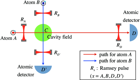
Figure 4: (Color online) Schematic of the proposal. The horizontal arrow is to describe the entangled state (1) generation (with $R_{A}$ and $C$) and measurement for atom $A$. The vertical arrow depicts the indirect parity measurement of the cavity field using ancillary atom $B$.

In this section, we discuss physical implementations of the Bell-CHSH inequality test using displaced parity measurements in a ‘circular Rydberg atom’-‘microwave cavity’ configuration. Generation schemes for atom-field entangled states (1) have been theoretically studied and experimentally implemented Brune1992 ; Davidovich1996 ; Haroche2006 ; Raimond2001 . In the case of a scheme based on the off-resonant interaction Haroche2006 , the required interaction Hamiltonian is

$$\hat{H}_{I}=\hbar\chi[(\hat{a}^{\dagger}\hat{a}+1)\left|e\right\rangle\left\langle e\right|-\hat{a}^{\dagger}\hat{a}\left|g\right\rangle\left\langle g\right|],$$ (16)

and $\chi=\Omega^{2}/(4\delta)$ is the coupling constant determined by the vacuum Rabi frequency $\Omega$ and detuning $\delta$ Haroche2006 . As shown in Fig. 4, $\pi/2$ Ramsey pulse with phase $-\pi/2$ ($R_{A}$) is applied to a circular Rydberg atom ($A$) prepared in the excited state $\left|e\right\rangle_{A}$ Nussenzveig1993 , which results in an atomic superposition state: $\left|\phi_{-i}\right\rangle_{A}=\left(\left|e\right\rangle_{A}-i\left|g\right\rangle_{A}\right)/{\sqrt{2}}$. Then, a strong dispersive interaction in Eq. (16) between atom $A$ and the cavity field produces the atom-field entangled state (1) for interaction time $t=\pi/(2\chi)$ Haroche2006 .

Direct measurements of the light field in the microwave cavity are difficult to achieve, while indirect methods for parity measurements of the cavity field may be more feasible Englert1993 ; MSKim2000 ; Haroche2006 ; Deleglise2008 . A circular Rydberg atom ($B$) in Fig. 4 initially prepared in state $\left|e\right\rangle_{B}$ evolves to a superposition state $\left|\phi_{-i}\right\rangle_{B}$ by $\pi/2$ Ramsey pulse with phase $-\pi/2$ ($R_{B}$), and the total state is $|\Psi_{tot}\rangle_{ABC}=\left|{\Psi}\right\rangle_{AC}\left|\phi_{-i}\right\rangle_{B}$. The displacement operation, $\hat{\cal D}^{\dagger}_{C}(\beta)=\hat{\cal D}_{C}(-\beta)$, is then applied to the field right before atom $B$ enters the cavity, and the same type of interaction as Eq. (16) between modes $B$ and $C$ follows. One may indirectly detect the cavity field by appropriately choosing the interaction time $t=\pi/(2\chi)$ between atom $B$ and the field before detecting the atom. The interaction time may be controlled by selecting the velocity of atom $B$. The final measurement for atom $A$, represented by $\hat{\Gamma}_{A}(-{\pi}e^{-i\phi}/4)$, is performed using $\pi/2$ Ramsey pulse of phase $\pi-\phi$ ($R_{D}$) and atomic detector $D$. The measurement on atom $B$, i.e., $\hat{\Gamma}_{B}(-\pi/4)$, for indirect probing is performed with the help of $\pi/2$ Ramsey pulse with $\pi$ phase ($R_{D^{\prime}}$) and atomic detector $D^{\prime}$. The measurement operator is then represented as

$$\hat{\Upsilon}_{B,C}(\beta,t)={\hat{\cal U}_{B,C}(\beta,t)}^{\dagger}\hat{\cal O}_{B,C}\hat{\cal U}_{B,C}(\beta,t),$$ (17)

where

$$\begin{split}&\hat{\cal O}_{B,C}=[\left|+\right\rangle\left\langle+\right|-\left|-\right\rangle\left\langle-\right|]_{B}\otimes{\openone}_{C},\\ &\hat{\cal U}_{B,C}=e^{-i\hat{H}_{I}t/\hbar}_{B,C}\hat{\cal D}_{C}^{{\dagger}}(\beta),\end{split}$$

and $\left|\pm\right>=(|e\rangle\pm|g\rangle)/\sqrt{2}$. The correlation function $E(\zeta,\beta,t)=\left\langle\hat{{\Gamma}}_{A}(\zeta)\otimes\hat{\Upsilon}_{B,C}(\beta,t)\right\rangle$ is calculated using state $|\Psi_{tot}\rangle_{ABC}$ as

$$\begin{split}E(\zeta,~{}\beta,~{}t)=&\frac{1}{2}\cos{\theta}e^{(|\alpha|^{2}+|\beta|^{2}-2|\alpha||\beta|\cos\Phi)(-1+\cos 2\chi t)}\cos[(|\alpha|^{2}+|\beta|^{2}-2|\alpha||\beta|\cos\Phi)\sin 2\chi t]\\ &-\frac{1}{2}\cos\theta e^{(|\alpha|^{2}+|\beta|^{2}+2|\alpha||\beta|\cos\Phi)(-1+\cos 2\chi t)}\cos[(|\alpha|^{2}+|\beta|^{2}+2|\alpha||\beta|\cos\Phi)\sin 2\chi t]\\ &+\frac{1}{2}\sin\theta e^{-|\alpha|^{2}-|\beta|^{2}-(|\alpha|^{2}-|\beta|^{2})\cos 2\chi t-2|\alpha||\beta|\sin\Phi\sin 2\chi t}\cos[\phi-(|\alpha|^{2}-|\beta|^{2})\sin 2\chi t+2|\alpha||\beta|\sin\Phi(-1+\cos 2\chi t)]\\ &+\frac{1}{2}\sin\theta e^{-|\alpha|^{2}-|\beta|^{2}-(|\alpha|^{2}-|\beta|^{2})\cos 2\chi t+2|\alpha||\beta|\sin\Phi\sin 2\chi t}\cos[\phi+(|\alpha|^{2}-|\beta|^{2})\sin 2\chi t+2|\alpha||\beta|\sin\Phi(-1+\cos 2\chi t)]\end{split}$$ (18)

and the Bell function, ${\cal B}_{\Upsilon}$, is accordingly obtained. As expected, the optimizing conditions for $|{\cal B}_{\Upsilon}|_{\rm max}$ are identical to those for $|{\cal B}_{\cal O}|_{\rm max}$ in Eqs. (14) and (15) with an additional condition, $t=t^{\prime}=\pi/2\chi$. Our numerical study confirms that the optimized Bell function $|{\cal B}_{\Upsilon}|_{\rm max}$ plotted with the abovementioned conditions in Fig. 5 exactly overlaps with the solid curve in Fig. 3 as shown . This result is due to the fact that the indirect measurement (17) is basically equivalent to the displaced parity measurement (12) on the cavity field when $t$ is chosen to be $\pi/(2\chi)$ Englert1993 . I.e., the measurement on atom $B$ in the basis $\{\left|+\right>,~{}\left|-\right>\}$ after the interaction time $t=\pi/(2\chi)$ is equivalent to the parity measurement on the cavity-field. In fact, it can be shown that the correlation functions (18) with $t=\pi/(2\chi)$ and (13) are identical. Of course, if we restrict $\zeta$ to be real, the optimized plot of the Bell function $|{\cal B}_{\Upsilon}|_{\rm max}$ approaches the dashed curve in Fig. 3.

Figure 5: Numerically optimized values of Bell function ${\cal B}_{\Upsilon}$ with indirect measurements against $|\alpha|$. The result is found to be identical to the one using direct parity measurements shown as the solid curve in Fig. 3.

V Decoherence and Loopholes

It is not difficult to predict that decoherence effects due to the cavity-field dissipation and the spontaneous emission of the atoms will obstruct Bell violations. This is particularly important when one intends to demonstrate a Bell violation free from the loopholes. In this section, we consider decoherence effects with realistic conditions for the Bell-CHSH inequality test using parity measurements and suggest quantitative requirements to perform a loophole-free Bell test.

V.1 Decoherence effects in the cavity-atom system

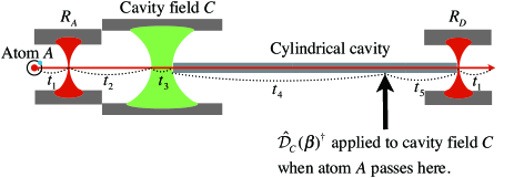
Figure 6: (Color online) Sideview of the atom $A$’s path with intervals of time. Each interval denotes an amount of time required for atom $A$ to pass through the region related with atomic velocity $v$. We note that the distance $l=v\times(t_{4}+t_{5})$, which corresponds to the length of the cylindrical cavity, is a crucial factor in a loohole-free Bell inequality test.

There are two main effects that cause decoherence in our Bell inequality test, i.e., spontaneous emissions from atoms and cavity field dissipations. In the atom-cavity system under consideration, one (or both) of these two effects may occur. The master equation which determines the time-evolution of the density operator, $\hat{\rho}(t)$, under the atom-field interaction with spontaneous emissions and cavity dissipations is

$$\frac{{d\hat{\rho}(t)}}{{dt}}=\frac{1}{{i\hbar}}[\hat{H}_{I},\hat{\rho}(t)]+{\cal L}\hat{\rho}(t),$$ (19)

with the Linblad decohering term $\cal L$ defined as

$$\begin{split}{\cal L}\hat{\rho}\equiv&\kappa(2\hat{a}\hat{\rho}\hat{a}^{\dagger}-\hat{a}^{\dagger}\hat{a}\hat{\rho}-\hat{\rho}\hat{a}^{\dagger}\hat{a})\\ &+{\gamma}(2\hat{\sigma}_{-}\hat{\rho}\hat{\sigma}_{+}-\hat{\sigma}_{+}\hat{\sigma}_{-}\hat{\rho}-\hat{\rho}\hat{\sigma}_{+}\hat{\sigma}_{-}),\end{split}$$ (20)

where $\kappa$ is the dissipation rate of cavity field, and $\gamma$ is the spontaneous emission rate.

It is known that the spontaneous emission rate of an atom can be significantly reduced by engineering the shape of the cavity that contains the atom Hulet1985 ; Kakazu1996 . A complete inhibition of spontaneous emission was suggested using a cylindrical metal cavity with a diameter shorter than ${1.8412c}/{\omega_{0}}$, where $\omega_{0}$ is the transition rate between atomic states $|e\rangle$ and $|g\rangle$ and $c$ is the speed of light Kakazu1996 . For our setup, the transition rate can be taken from Ref. Deleglise2008 as $\omega_{0}=51.1\rm{GHz}$. This means that the diameter should be smaller than $3.44\rm{mm}$ that is experimentally achievable. As seen in Fig. 6, a long cylindrical cavity may be used between cavity $C$ and Ramsey zone $R_{D}$ to inhibit spontaneous emission.

The spontaneous emission rate $\gamma_{c}$ inside the cavity $C$ in Fig. 4 is also generally different from the spontaneous emission rate $\gamma_{0}$ in the vacuum. It is known that $\gamma_{c}$ can be calculated by approximating the cavity in the one dimension while considering the effect of the atomic motion as described in Ref. Wilkens1992 . In our case, $\gamma_{c}=\rm{4.08~{}Hz}$ is obtained based on the result of Ref. Wilkens1992 from the spontaneous emission rate in the vacuum, $\gamma_{0}=1/(2T_{0})$ ($T_{0}=\rm{36~{}ms}$ is the atomic life time in the vacuum Haroche2006 ) and related realistic parameters in a recent experiment Deleglise2008 .

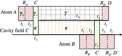
Figure 7: (Color online) A timeline for decoherence with dynamical parameters related in each regions (from left to right). The top line is for atom $A$, the middle for cavity field $C$, and the bottom for atom $B$. The times when Ramsey pulses are applied are described as vertical dashed lines. We consider a Ramsey pulse application as an instant event as a Ramsey pulse lasts as short as $\rm{1~{}\mu s}$ order Raimond2001 . Regions are differently hatched depending on the types of dynamics. In the diagonally hatched regions, atoms $A$ and $B$ travel in free spaces with the spontaneous emission rate $\gamma_{0}$ before and after Ramsey pulses as shown in Fig. 4. In the cross-hatched region, atom $A$ travels in a cylindrical cavity with the inhibited spontaneous emission rate $\gamma^{\prime}$. In the vertically hatched region, the cavity dissipation with rate $\kappa$ occurs in the cavity ($C$) field. The horizontally hatched regions correspond to the dynamics of the atom-field interaction $\hat{H}_{I}$ in the main cavity $C$ together with spontaneous emission $\gamma_{c}$ and cavity dissipation $\kappa$. Abbreviations $C$, $D$, $D^{\prime}$, $R_{A}$, $R_{B}$, $R_{D}$, and $R_{D^{\prime}}$ are consistent with those in Fig. 4.

Considering the discussions above, we present a timeline of decoherence effects in Fig. 7 together with time intervals required to pass through certain parts of the apparatus as follows (also depicted in Fig. 6):  $t_{1}$ is a half of the time required for an atom to pass through a cavity used for Ramsey pulse application, $t_{2}$ is a half of the time required for an atom to pass through Ramsey pulse and the main cavity (C) without cavity waist, $t_{3}$ for an atom to pass through the main cavity(C)’s waist ($\pi/2\chi$), $t_{4}$ for atom $A$ to pass through the long cylindrical cavity before the field displacement operation on the cavity field, $t_{5}$ for atom $A$ to pass through the remainder of the long cavity after the field displacement operation, and $t_{6}$ for atomic detection at $D$ or $D^{\prime}$.

Let us first consider the pathway of atom A, which corresponds to the top line of Fig. 7. Atom $A$ undergoes spontaneous emission before and after the Ramsey pulse $R_{A}$ with rate $\gamma_{0}$ (diagonally hatched part). Atom $A$ then interacts with the cavity field with dissipation rate $\kappa$ under spontaneous emission ($\gamma_{c}$), which is represented by the horizontally hatched part. After the atom-field interaction, atom $A$ passes through the cylindrical cavity experiencing inhibited spontaneous emission ($\gamma^{\prime}$). Finally, atom $A$ comes out of Ramsey pulse $R_{D}$ experiencing spontaneous emission ($\gamma_{0}$), and is registered at detector $D$. In the mean while, cavity field $C$ which have interacted with atom $A$ undergoes field dissipation ($\kappa$) while atom $A$ is passing through cylindrical cavity. Then, cavity field $C$ begins to interacts with atom $B$ under spontaneous emission ($\gamma_{c}$) and field dissipation ($\kappa$) after displacement operation on it. Atom $B$, used for an indirect measurement, experiences spontaneous emission ($\gamma_{0}$) around Ramsey pulse $R_{B}$, interaction with the cavity field ($C$) with spontaneous emission ($\gamma_{c}$), and spontaneous emission ($\gamma_{0}$) before detection $D^{\prime}$.

Here, we take the photon storage time $T_{C}=\rm{0.13~{}s}$ ($\kappa=1/(2T_{C})$), $\Omega=2\pi\cdot\rm{49~{}kHz}$ and $\delta=2\pi\cdot\rm{65~{}kHz}$ ($\chi=\Omega^{2}/(4\delta)\approx 58{\rm kHz}$) from recent experiments Deleglise2008 . The solution of the master equation for the cavity dissipation alone with $H_{I}$, was examined in Ref. Faria1999May . In Appendix, we obtain the solution of Eq. (19) and find an explicit form of the density operator and the correlation function. The Bell function can be constructed using the correlation function in Eq. (54) of Appendix. Note that we have assumed perfect Ramsey pulses during the procedures. Considering cavity dissipation, we employ the same optimizing conditions (14) except that $|\beta|$ is chosen to be the values that satisfy

$$\frac{|\alpha|e^{-\kappa(t_{4}+t_{3})}-|\beta|}{|\alpha|e^{-\kappa(t_{4}+t_{3})}+|\beta|}=\tan({4|\alpha|e^{-\kappa(t_{4}+t_{3})}|\beta|}),$$ (21)

and is nearest to zero.

V.2 Bell violation and separations under practical conditions without a cylindrical cavity

Let us first consider Bell violation depending on the separation $l=v\times(t_{4}+t_{5})$ between both parties without using a cylindrical cavity (thus $\gamma^{\prime}=\gamma_{0}$). We choose some practical time-interval parameters as $t_{1}=\rm{80.0~{}\mu s}$, $t_{2}=\rm{166.5~{}\mu s}$, $t_{3}=\rm{27.1~{}\mu s}$, $t_{6}=\rm{20~{}\mu s}$ and velocity of an atom $v=\rm{250~{}m/s}$ Deleglise2008 ; Zhou2009P . The Bell function with several choices of $l$ are plotted in Fig. 8. The Bell function approaches the value near 2.7 when $l=0.1$(meter), but it decreases as $l$ gets larger. Clear Bell violations appear for $l\lesssim 2$(meter), however, this is insufficient for a space-like separation as we shall discuss in the next subsection.

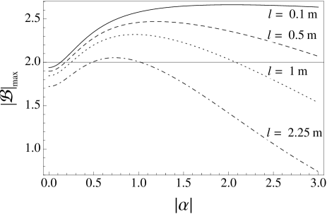
Figure 8: The Bell function under realistic conditions discussed in Sec. V.2 are plotted with optimizing conditions in Eqs. (14) and (21) for several different cases of separation $l$. As the separation $l$ gets larger, the maximum values of the Bell function decrease. The decoherence effects become heavier as $|\alpha|$ gets larger.

V.3 Requirements for a Bell test free from the locality loophole with a cylindrical cavity

In principle, a Bell test free from the locality loophole can be performed using a long cylindrical cavity with a low spontaneous emission rate ($\gamma^{\prime}$) and the main cavity with a low dissipation rate ($\kappa$). In order to close the locality loophole, the measurement event for atom $A$ should not affect the measurement event for the cavity field $C$, and vice versa Bell1981 . In other words, the measurement event for atom $A$ should be outside of the “back light cone” from the detection event $D^{\prime}$ in Fig. 4. In the same manner, the measurement event for the cavity field $C$ should not be in the back light cone from the detection event $D$. For simplicity, let us first suppose that each measurement process takes place at a single location ($D$ and $D^{\prime}$). In our Bell test, the time $t_{A}$ required to measure atom $A$ is smaller than the time required to measure field $C$ ($t_{C}$) due to the indirect measurement scheme for field $C$. We assume that the measurement event for the field $C$ precedes to the measurement event for atom $A$ by $T$ (the opposite case will require a longer separation between the two parties). Then the conditions required to close the locality loophole are

$$\begin{split}d\geq c(T+t_{A}),\\ d\geq c(t_{C}-T),\end{split}$$ (22)

where $d$ is the distance between $D$ and $D^{\prime}$ and $c$ is the speed of light.

In order to apply the locality-loophole-free conditions (22) to our Bell test setup in a more rigorous manner, one needs to consider locations of the local measurement elements. In Fig. 7, one can find that the measurement time for atom $A$ ($t_{A}$) consists of the times for $R_{D}$ ($t_{1}$) and $D$ ($t_{6}$) and that for the field ($t_{C}$) consists of the times for $C$ ($t_{3}$), $R_{D}^{\prime}$ ($t_{2}+t_{1}$), and $D^{\prime}$ ($t_{6}$). A measurement event for each party actually does not take place at a single location, and both of the measurements are not even on a straight line. Therefore the distance $d$ in Eqs. (22) needs to be replaced with the distances from the final detector of one party to the location where the measurement of the other party begins. A careful consideration leads to the conclusion that the following inequalities should be satisfied:

$$\begin{split}&v(t_{3}/2+t_{4}+t_{5}+t_{1}+t_{6})\geq c(t_{5}+t_{1}+t_{6}),\\ &v\sqrt{(t_{3}/2+t_{2}+t_{1}+t_{6})^{2}+(t_{3}/2+t_{4}+t_{5})^{2}}\\ &~{}~{}~{}~{}~{}~{}~{}~{}~{}~{}\geq c(t_{3}+t_{2}+t_{1}+t_{6}-t_{5}).\end{split}$$ (23)

Using the feasible values of $t_{1}$, $t_{2}$, $t_{3}$, $t_{6}$ and $v$ in the previous subsection, we find the minimum values $t_{4}=236.0~{}s$ and $t_{5}=96.8~{}\rm{\mu s}$ with which the equalities hold for Eqs. (23). Then, the minimum distance required for a Bell test free from the locality loophole is found to be $l=\rm{52.99~{}km}$ Deleglise2008 .

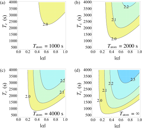
Figure 9: (Color online) Contour plots of the Bell function with respect to photon storage time $T_{C}$ in the main cavity and amplitude $|\alpha|$ of the entangled state. The atomic life time in cylindrical cavity $T_{\rm atom}$ is fixed at 1000, 2000, 4000 and $\infty$ (seconds). The minimum distance condition $l=52.99$ (km) for a loophole-free Bell test was assumed. Higher inhibition of spontaneous emission in the cylindrical cavity reduces the required photon storage time in the main cavity.

We finally consider conditions of the atomic life time $T_{\rm{atom}}=1/(2\gamma^{\prime})$ and the photon storage time $T_{c}=1/(2\kappa)$ required for a Bell test free from the locality loophole. In Fig. 9, we plot the Bell function constructed using Eq. (54) in Appendix with respect to the photon storage time in the main cavity and amplitude $|\alpha|$ of the atom-field entanglement. Here, the extended lifetime of the atom in the cylindrical cavity was assumed to be $T_{\rm atom}=$1000, 2000, 4000, and $\infty$ (seconds). The distance $l$ was assumed to be the minimum distance required for a loophole-free Bell test ($52.99$ km). For example, when $T_{\rm atom}=2000$ (seconds), the photon storage time $T_{C}\sim 1160$ (seconds) at $|\alpha|\sim 0.47$ is required to see a Bell violation. If complete inhibition of the spontaneous emission in the cylindrical cavity is possible, (i.e., $T_{\rm atom}=\infty$), $T_{C}\sim 590$ at $|\alpha|\sim 0.3$ is required. Obviously, the stronger inhibition of the spontaneous emission in the cylindrical cavity relaxes the requirement of the photon storage time in the main cavity to see Bell violations. However, it still requires at least a few hundreds of seconds for the photon storage time to demonstrate a loophole-free Bell violation, while it is only about $0.13~{}{\rm{s}}$ at present Kuhr2007 . It would also be extremely challenging to build a long cylindrical cavity that strongly inhibits the spontaneous emission of atom $A$ during such a long life time.

VI Remarks

We have investigated Bell-CHSH inequality tests with entanglement between a two-level atom and a coherent-state field in a cavity. In order to detect the cavity field for these tests, photon on/off measurements and photon number parity measurements, respectively, have been attempted. When photon on/off measurements with the perfect efficiency are used, the maximum value of the Bell violation is ${\cal B}_{\cal O}\approx 2.61$ at $|\alpha|\approx 0.664$. In order to see a violation of the Bell-CHSH inequality, at least 50% of detection efficiency is required. When photon parity measurements are used, the value of the Bell-CHSH violation rapidly increases as $\alpha$ gets larger, and it approaches Cirel’son’s bound for $\alpha\gg 1$. Although precise direct measurements of cavity fields are experimentally difficult, photon number parity measurements for the cavity field can be effectively performed using ancillary probe atoms and atomic detectors. We have fully analyzed decoherence effects in both field and atomic modes and discuss conditions required to perform a Bell inequality test free from the locality loophole.

Our proposal may be considered an attempt to analyze a Bell inequality test using entanglement between a microscopic system and a mesoscopic classical system. Since atomic detectors are known to be highly efficient Maioli2005 , it may also be a reasonable target to perform this type of experiment in a way free from the detection loophole. In principle, a Bell inequality test free from the locality loophole in our framework using atom-field entanglement may be performed using a long cylindrical cavity for the atom with a low spontaneous emission rate Kakazu1996 . However, our analysis shows that it would be extremely demanding to perform a Bell inequality test free from both the locality and detection loopholes in this framework since the main cavity for field with a low dissipation rate would be necessary together with a long cylindrical cavity.

Appendix A Solutions of the Master Equation for Matrix Elements

We first find general solutions of the master equation (19) for three types of decoherence processes step by step, i.e., spontaneous emission of an atom, cavity dissipation, and atom-field interaction with spontaneous emission and cavity dissipation.

A.1 Spontaneous emission for atom

A density operator of a two-level atom, $\hat{\rho}_{A}(t)$, can be expressed as a matrix form

$$\hat{\rho}_{A}(t)=\left({\begin{array}[]{*{20}c}{\rho_{A,ee}(t)}&{\rho_{A,eg}(t)}\\ {\rho_{A,ge}(t)}&{\rho_{A,gg}(t)}\\ \end{array}}\right),$$ (24)

where ${\rho_{A,ij}(t)}=\left\langle i\right|\hat{\rho}_{A}(t)\left|j\right\rangle$. When an atom with a initial density matrix, $\hat{\rho}_{A}(0)$, goes through the spontaneous emission process for time $t$, its density matrix is straightforwardly obtained using Eq. (19) with $\chi=0$ and $\kappa=0$ as

$$\begin{split}\hat{\rho}_{A}(t)=&{\hat{\cal S}}_{A}(\gamma,t)[\hat{\rho}_{A}(0)]\\ =&\left({\begin{array}[]{*{20}c}{e^{-2\gamma t}\rho_{A,ee}(0)}&{e^{-\gamma t}\rho_{A,eg}(0)}\\ {e^{-\gamma t}\rho_{A,ge}(0)}&{\rho_{A,gg}(0)-\rho_{A,ee}(0)(e^{-2\gamma t}-1)}\\ \end{array}}\right),\end{split}$$ (25)

where superoperator $\hat{\cal S}(\gamma,t)$ is defined for later use.

A.2 Dissipation for cavity field

In order to find the time evolution of the coherent-state part the density operator, it is sufficient to find the time evolution of an operator component $\left|\mu\right\rangle\left\langle\nu\right|$, where $\left|\mu\right\rangle$ and $\left|\nu\right\rangle$ are coherent states of amplitudes $\mu$ and $\nu$. This solution for time $t$ under the master equation (19) with $\chi=0$ and $\gamma=0$ is well known as Phoenix ; Moya-Cessa2006Aug

$$\exp[-\frac{({\left|\mu\right|}^{2}+{\left|\nu\right|}^{2}-2\nu^{*}\mu)(1-\exp(-2\kappa t))}{2}]\left|\mu e^{-\kappa t}\right\rangle\left\langle\nu e^{-\kappa t}\right|.$$ (26)

A.3 Atom-field interaction with spontaneous emission and cavity dissipation

The density matrix $\hat{\rho}(t)$ for an atom-field state can be considered in a $2\times\infty$ dimensional space, since we assume a two-level atom. It is possible to decompose the master equation (19) in $\{\left|e\right\rangle,~{}\left|g\right\rangle\}$ basis with the density matrix elements ${\hat{\rho}_{C,ij}(t)}=\left\langle i\right|\hat{\rho}(t)\left|j\right\rangle$. We then obtain equations

$$\begin{split}\frac{d}{{dt}}\hat{\rho}_{C,ee}=&{\hat{\cal{L}}}_{ee}\hat{\rho}_{C,ee}-2\gamma\hat{\rho}_{C,ee}\\ =&-i\chi[\hat{a}^{\dagger}\hat{a},\hat{\rho}_{C,ee}]+\kappa(2\hat{a}\hat{\rho}_{C,ee}\hat{a}^{\dagger}-\hat{a}^{\dagger}\hat{a}\hat{\rho}_{C,ee}-\hat{\rho}_{C,ee}\hat{a}^{\dagger}\hat{a})\\ &-2\gamma\hat{\rho}_{C,ee},\\ \end{split}$$ (27)

$$\begin{split}\frac{d}{{dt}}\hat{\rho}_{C,gg}=&{\hat{\cal{L}}}_{gg}\hat{\rho}_{C,gg}+2\gamma\hat{\rho}_{C,ee}\\ =&i\chi[\hat{a}^{\dagger}\hat{a},\hat{\rho}_{C,gg}]+\kappa(2\hat{a}\hat{\rho}_{C,gg}\hat{a}^{\dagger}-\hat{a}^{\dagger}\hat{a}\hat{\rho}_{C,gg}-\hat{\rho}_{C,gg}\hat{a}^{\dagger}\hat{a})\\ &+2\gamma\hat{\rho}_{C,ee},\\ \end{split}$$ (28)

$$\begin{split}\frac{d}{{dt}}\hat{\rho}_{C,eg}=&{\hat{\cal{L}}}_{eg}\hat{\rho}_{C,eg}-i\chi\hat{\rho}_{C,eg}-\gamma\hat{\rho}_{C,eg}\\ =&-i\chi(\hat{a}^{\dagger}\hat{a}+1)\hat{\rho}_{C,eg}-i\chi\hat{\rho}_{C,eg}\hat{a}^{\dagger}\hat{a}\\ &+\kappa(2\hat{a}\hat{\rho}_{C,eg}\hat{a}^{\dagger}-\hat{a}^{\dagger}\hat{a}\hat{\rho}_{C,eg}-\hat{\rho}_{C,eg}\hat{a}^{\dagger}\hat{a})-\gamma\hat{\rho}_{C,eg},\\ \end{split}$$ (29)

$$\begin{split}\frac{d}{{dt}}\hat{\rho}_{C,ge}=&{\hat{\cal{L}}}_{ge}\hat{\rho}_{C,ge}+i\chi\hat{\rho}_{C,ge}-\gamma\hat{\rho}_{C,ge}\\ =&i\chi\hat{\rho}_{C,ge}(\hat{a}^{\dagger}\hat{a}+1)+i\chi\hat{a}^{\dagger}\hat{a}\hat{\rho}_{C,ge}\\ &+\kappa(2\hat{a}\hat{\rho}_{C,ge}\hat{a}^{\dagger}-\hat{a}^{\dagger}\hat{a}\hat{\rho}_{C,ge}-\hat{\rho}_{C,ge}\hat{a}^{\dagger}\hat{a})-\gamma\hat{\rho}_{C,ge}.\end{split}$$ (30)

We define the following superoperators for simplicity: ${\hat{\cal{M}}}=\hat{a}^{\dagger}\hat{a}~{}\cdot~{}$ , ${\hat{\cal{P}}}=~{}\cdot~{}\hat{a}^{\dagger}\hat{a}$ , and ${\hat{\cal{J}}}=\hat{a}~{}\cdot~{}\hat{a}^{\dagger}$ . Then ${\hat{\cal{L}}}_{ee}$, ${\hat{\cal{L}}}_{gg}$, ${\hat{\cal{L}}}_{eg}$, and ${\hat{\cal{L}}}_{ge}$ can be expressed as,

$${\hat{\cal{L}}}_{ee} \equiv 2\kappa{\hat{\cal{J}}}-r{\hat{\cal{M}}}-r^{*}{\hat{\cal{P}}},$$ (31a)

$${\hat{\cal{L}}}_{eg} \equiv 2\kappa{\hat{\cal{J}}}-r{\hat{\cal{M}}}-r{\hat{\cal{P}}},$$ (31b)

where $r\equiv\kappa+i\chi$, and ${\hat{\cal{L}}}_{gg}$ and ${\hat{\cal{L}}}_{ge}$ are obtained by substituting $\chi$ with $-\chi$ in ${\hat{\cal{L}}}_{ee}$, and ${\hat{\cal{L}}}_{eg}$, respectively. A master equation of the form ${d\hat{\rho}}/{dt}=\hat{\cal L}\hat{\rho}+c\hat{\rho}$, where $c$ is a constant and $\hat{\cal L}$ is a superoperator, can be solved with a usual exponential form $\exp{[(\hat{\cal L}+c)t]}\hat{\rho}$.

A.3.1 Solution for ${\hat{\rho}}_{C,ee}$

The solution of Eq. (27) is

$$\hat{\rho}_{C,ee}(t)=\exp[(\hat{\cal L}_{ee}-2\gamma)t]\hat{\rho}_{C,ee}(0)=e^{-2\gamma t}e^{\hat{\cal L}_{ee}t}\hat{\rho}_{C,ee}(0).$$ (32)

where the factorization can be done by the similarity transformation Witschel1981 . Now we need to factorize $e^{\hat{\cal L}_{ee}t}$. This is solved with an ansatz (a technique can be found in Ref. Moya-Cessa2006Aug )

$$\hat{\rho}_{C,ee}(t)=\exp[-2\gamma t]\exp[(-r{\hat{\cal{M}}}-r^{*}{\hat{\cal{P}}})t]\exp[f(t)2\kappa{\hat{\cal{J}}}]\hat{\rho}_{C,ee}(0),$$ (33)

where $f(t)=(1-e^{-2\kappa t})/(2\kappa)$. For an initial state $\hat{\rho}_{C,ee}(0)=\left|\mu\right\rangle\left\langle\nu\right|$,

$$\hat{\rho}_{C,ee}(t)=\exp[-2\gamma t+\Theta(\kappa,0,\mu,\nu,t)]\left|\mu e^{-rt}\right\rangle\left\langle\nu e^{-rt}\right|$$ (34)

with

$$\Theta(\kappa,\chi,\mu,\nu,t):=-\frac{1}{2}({\left|\nu\right|}^{2}+{\left|\mu\right|}^{2})(1-e^{-2\kappa t})+\frac{\kappa}{r}(1-e^{-2rt})\nu^{*}\mu.$$ (35)

A.3.2 Solution for ${\hat{\rho}}_{C,gg}$

In order to solve Eq. (28), we first assume $\gamma=0$. A homogeneous solution is obtained from Eq. (34) by substituting $\chi$ with $-\chi$ as

$$\hat{\rho}_{C,gg}^{h}(t)=\exp[\Theta(\kappa,0,\mu,\nu,t)]\left|\mu e^{-r^{*}t}\right\rangle\left\langle\nu e^{-r^{*}t}\right|.$$ (36)

Then it is obvious to see that the general solution $\hat{\rho}_{C,gg}(t)$ with $\gamma\neq 0$ is

$$\begin{split}\hat{\rho}_{C,gg}(t)&=\hat{\rho}_{C,gg}^{h}(t)+2\gamma\int_{0}^{t}{dt^{\prime}\hat{\rho}_{C,ee}(t^{\prime})}\\ &=\exp[\Theta(\kappa,0,\mu,\nu,t)]\left|\mu e^{-r^{*}t}\right\rangle\left\langle\nu e^{-r^{*}t}\right|\\ &+2\gamma\int_{0}^{t}{dt^{\prime}\exp[-2\gamma t^{\prime}+\Theta(\kappa,0,\mu,\nu,t^{\prime})]}\left|{\mu e^{-rt^{\prime}}}\right\rangle\left\langle{\nu e^{-rt^{\prime}}}\right|.\end{split}$$ (37)

A.3.3 Solution for ${\hat{\rho}}_{C,ge}$

The solution of Eq. (30) is

$$\hat{\rho}_{C,ge}(t)=\exp[(\hat{\cal L}_{ge}+i\chi-\gamma)t]\hat{\rho}_{C,ge}(0)=e^{(i\chi-\gamma)t}e^{\hat{\cal L}_{ge}t}\hat{\rho}_{C,ge}(0).$$ (38)

Factoring $e^{\hat{\cal L}_{eg}t}$ with an ansatz

$$\hat{\rho}_{C,ge}(t)=\exp[(i\chi-\gamma)t]\exp[(-r{\hat{\cal{M}}}-r^{*}{\hat{\cal{P}}})t]\exp[g(t)2\kappa{\hat{\cal{J}}}]\hat{\rho}_{C,ee}(0),$$ (39)

where $g(t)=(1-e^{-2r^{*}t})/(2r^{*})$. For $\hat{\rho}_{C,ge}(0)=\left|\mu\right\rangle\left\langle\nu\right|$,

$$\hat{\rho}_{C,ge}(t)=\exp[(i\chi-\gamma)t+\Theta(\kappa,-\chi,\mu,\nu,t)]\left|\mu e^{-r^{*}t}\right\rangle\left\langle\nu e^{-rt}\right|.$$ (40)

A.3.4 Solution for ${\hat{\rho}}_{C,eg}$

The solution of Eq. (29) is obtained from Eq. (40) by substituting $\chi$ with $-\chi$ as

$$\hat{\rho}_{C,eg}(t)=\exp[(-i\chi-\gamma)t+\Theta(\kappa,\chi,\mu,\nu,t)]\left|\mu e^{-rt}\right\rangle\left\langle\nu e^{-r^{*}t}\right|.$$ (41)

Appendix B Derivation of the density matrices for atom-field entanglement and the correlation function

B.1 Atom-field entanglement generated under decoherence effects

First, atom $A$ initially prepared in $|e\rangle_{A}$ undergoes the spontaneous emission for the time $t_{1}$. After applying the first Ramsey pulse, $R_{A}=\hat{D}_{A}(-i\pi/4)$, explained in Sec. IV, atom $A$ again undergoes the spontaneous emission for time $t_{2}$. Using Eqs. (25) again, it becomes

$$\begin{split}&\hat{\cal S}_{A}(\gamma_{0},t_{2})\Big{[}\hat{D}_{A}(-i\pi/4)|\Big{\{}\hat{\cal S}_{A}(\gamma_{0},t_{1})[(|e\rangle\langle e|)_{A}]\Big{\}}\hat{D}^{\dagger}_{A}(-i\pi/4)\Big{]}\\ &~{}=\left({\begin{array}[]{*{20}c}{\frac{1}{2}e^{-2\gamma_{0}t_{2}}}&{(-\frac{i}{2}+ie^{-2\gamma_{0}t_{1}})e^{-\gamma_{0}t_{2}}}\\ {(\frac{i}{2}-ie^{-2\gamma_{0}t_{1}})e^{-\gamma_{0}t_{2}}}&{(1-\frac{1}{2}e^{-2\gamma_{0}t_{2}})}\\ \end{array}}\right).\end{split}$$ (42)

Then atom $A$ interacts with the cavity field $C$ prepared in state $|i\alpha\rangle_{C}$. Using Eqs. (34), (37), (40) and (41), we find the state after the interaction time $t_{3}$ as $\hat{\rho}_{AC}^{(3)}$ with its matrix elements:

$$\begin{split}\hat{\rho}_{AC,ee}^{(3)}=\frac{1}{2}e^{-2\gamma_{0}t_{2}-2\gamma_{c}t_{3}}\left|{i\alpha e^{-rt_{3}}}\right\rangle\left\langle{i\alpha e^{-rt_{3}}}\right|,\end{split}$$ (43a)

$$\begin{split}&\hat{\rho}_{AC,eg}^{(3)}=(-\frac{i}{2}+ie^{-2\gamma_{0}t_{1}})\exp[-\gamma_{0}t_{2}+(-i\chi-\gamma_{c})t_{3}\\ &+\Theta(\kappa,\chi,\alpha,\alpha,t_{3})]\left|{i\alpha e^{-rt_{3}}}\right\rangle\left\langle{i\alpha e^{-r^{*}t_{3}}}\right|,\end{split}$$ (43b)

$$\begin{split}&\hat{\rho}_{AC,ge}^{(3)}=(\frac{i}{2}-ie^{-2\gamma_{0}t_{1}})\exp[-\gamma_{0}t_{2}+(i\chi-\gamma_{c})t_{3}\\ &+\Theta(\kappa,-\chi,\alpha,\alpha,t_{3})]\left|{i\alpha e^{-r^{*}t_{3}}}\right\rangle\left\langle{i\alpha e^{-rt_{3}}}\right|,\end{split}$$ (43c)

$$\begin{split}&\hat{\rho}_{AC,gg}^{(3)}=(1-\frac{1}{2}e^{-2\gamma_{0}t_{2}})\left|{i\alpha e^{-r^{*}t_{3}}}\right\rangle\left\langle{i\alpha e^{-r^{*}t_{3}}}\right|\\ &+2\gamma_{c}\int_{0}^{t_{3}}{dt}\frac{1}{2}e^{-2\gamma_{0}t_{2}-2\gamma_{c}t}\left|{i\alpha e^{-rt}}\right\rangle\left\langle{i\alpha e^{-rt}}\right|.\end{split}$$ (43d)

B.2 Atom-field entanglement after traveling for the spacelike separation

We now derive the total density matrix right before $\hat{\cal D}_{C}^{{\dagger}}(\beta)$ is applied. The state $\hat{\rho}_{AC}^{(3)}$ undergoes spontaneous emission inside the cylindrical cavity and dissipation inside the cavity field $C$. The calculation can be done using the results in Sec. A.3 with $\chi=0$. Then the state becomes $\hat{\rho}_{AC}^{(4)}$, where

$$\begin{split}\hat{\rho}_{AC,ee}^{(4)}=\frac{1}{2}e^{-2\gamma_{0}t_{2}-2\gamma_{c}t_{3}-2\gamma^{\prime}t_{4}}\left|{i\alpha e^{-rt_{3}-\kappa t_{4}}}\right\rangle\left\langle{i\alpha e^{-rt_{3}-\kappa t_{4}}}\right|,\end{split}$$ (44a)

$$\begin{split}\hat{\rho}_{AC,eg}^{(4)}&=(-\frac{i}{2}+ie^{-2\gamma_{0}t_{1}})\exp[-\gamma_{0}t_{2}+(-i\chi-\gamma_{c})t_{3}-\gamma^{\prime}t_{4}\\ &+\Theta(\kappa,\chi,\alpha,\alpha,t_{3})+\Theta(\kappa,0,\alpha e^{-rt_{3}},\alpha e^{-r^{*}t_{3}},t_{4})]\\ &\left|{i\alpha e^{-rt_{3}-\kappa t_{4}}}\right\rangle\left\langle{i\alpha e^{-r^{*}t_{3}-\kappa t_{4}}}\right|,\end{split}$$ (44b)

$$\begin{split}\hat{\rho}_{AC,ge}^{(4)}&=(\frac{i}{2}-ie^{-2\gamma_{0}t_{1}})\exp[-\gamma t_{2}+(i\chi-\gamma_{c})t_{3}-\gamma^{\prime}t_{4}\\ &+\Theta(\kappa,-\chi,\alpha,\alpha,t_{3})+\Theta(\kappa,0,\alpha e^{-r^{*}t_{3}},\alpha e^{-rt_{3}},t_{4})]\\ &\left|{i\alpha e^{-r^{*}t_{3}-\kappa t_{4}}}\right\rangle\left\langle{i\alpha e^{-rt_{3}-\kappa t_{4}}}\right|,\end{split}$$ (44c)

$$\begin{split}\hat{\rho}_{AC,gg}^{(4)}&=(1-\frac{1}{2}e^{-2\gamma_{0}t_{2}})\left|{i\alpha e^{-r^{*}t_{3}-\kappa t_{4}}}\right\rangle\left\langle{i\alpha e^{-r^{*}t_{3}-\kappa t_{4}}}\right|\\ &+2\gamma_{c}\int_{0}^{t_{3}}{dt}\frac{1}{2}e^{-2\gamma_{0}t_{2}-2\gamma_{c}t}\left|{i\alpha e^{-rt-\kappa t_{4}}}\right\rangle\left\langle{i\alpha e^{-rt-\kappa t_{4}}}\right|\\ &+2\gamma^{\prime}\int_{0}^{t_{4}}{dt}\frac{1}{2}e^{-2\gamma_{0}t_{2}-2\gamma_{c}t_{3}-2\gamma^{\prime}t}\left|{i\alpha e^{-rt_{3}-\kappa t}}\right\rangle\left\langle{i\alpha e^{-rt_{3}-\kappa t}}\right|,\end{split}$$ (44d)

and here the subscripts are consistent with the previous ones.

B.3 Effects with atom $B$ for indirect measurement

After applying the displacement operation $\hat{\cal D}_{C}^{{\dagger}}(\beta)$, the total state becomes $\hat{\rho}_{AC}^{\beta}=\hat{\cal D}_{C}^{{\dagger}}(\beta)\hat{\rho}_{AC}^{l}\hat{\cal D}_{C}(\beta)$. Now, the probe atom $B$, which is in the same state as that of atom $A$ in Eq. (42), goes into the cavity field of state $\hat{\rho}_{AC}^{\beta}$. The atom-field interaction $H_{I}$ with the coupling constant $\chi$ occurs between atom $B$ and field $C$ for time $t_{3}$. When solving the master equation, it is convenient if one notes that the field-part of state $\hat{\rho}_{AC}^{\beta}$ can be expressed by coherent-state dyadics such as $|\mu\rangle\langle\nu|$. If the component of the cavity field, initially prepared as $|\mu\rangle\langle\nu|$, interacts with an atomic state (42) for time $t_{3}$, the resulting density operator element is obtained as $\hat{\Omega}_{BC}(\mu,\nu,t_{3})$ with

$$\begin{split}\hat{\Omega}_{BC,ee}(\mu,\nu,t_{3})=\frac{1}{2}e^{-2\gamma_{0}t_{2}-2\gamma_{c}t_{3}+\Theta(\kappa,0,\mu,\nu,t_{3})}\left|{\mu e^{-rt_{3}}}\right\rangle\left\langle{\nu e^{-rt_{3}}}\right|,\end{split}$$ (45a)

$$\begin{split}&\hat{\Omega}_{BC,eg}(\mu,\nu,t_{3})=(-\frac{i}{2}+ie^{-2\gamma_{0}t_{1}})\exp[-\gamma_{0}t_{2}+(-i\chi-\gamma_{c})t_{3}\\ &+\Theta(\kappa,\chi,\mu,\nu,t_{3})]\left|{\mu e^{-rt_{3}}}\right\rangle\left\langle{\nu e^{-r^{*}t_{3}}}\right|,\end{split}$$ (45b)

$$\begin{split}&\hat{\Omega}_{BC,ge}(\mu,\nu,t_{3})=(\frac{i}{2}-ie^{-2\gamma_{0}t_{1}})\exp[-\gamma_{0}t_{2}+(i\chi-\gamma_{c})t_{3}\\ &+\Theta(\kappa,-\chi,\mu,\nu,t_{3})]\left|{\mu e^{-r^{*}t_{3}}}\right\rangle\left\langle{\nu e^{-rt_{3}}}\right|,\end{split}$$ (45c)

$$\begin{split}&\hat{\Omega}_{BC,gg}(\mu,\nu,t_{3})=(1-\frac{1}{2}e^{-2\gamma_{0}t_{2}})e^{\Theta(\kappa,0,\mu,\nu,t_{3})}\left|{\mu e^{-r^{*}t_{3}}}\right\rangle\left\langle{\nu e^{-r^{*}t_{3}}}\right|\\ &+2\gamma_{c}\int_{0}^{t_{3}}{dt}\frac{1}{2}e^{-2\gamma_{0}t_{2}-2\gamma_{c}t+\Theta(\kappa,0,\mu,\nu,t)}\left|{\mu e^{-rt}}\right\rangle\left\langle{\nu e^{-rt}}\right|.\end{split}$$ (45d)

We used Eqs. (34), (37), (40) and (41) again to find Eqs. (45a)-(45d). Therefore, $\hat{\rho}_{AC}^{\beta}$ interacts with atom $B$ and evolves to

$$\begin{split}\hat{\rho}_{ABC}=&(|e\rangle\langle e|)_{A}\otimes\hat{\rho}_{BC,ee}+(|e\rangle\langle g|)_{A}\otimes\hat{\rho}_{BC,eg}\\ &+(|g\rangle\langle e|)_{A}\otimes\hat{\rho}_{BC,ge}+(|g\rangle\langle g|)_{A}\otimes\hat{\rho}_{BC,gg},\end{split}$$ (46)

where

$$\begin{split}\hat{\rho}_{BC,ee}=&\frac{1}{2}e^{-2\gamma_{0}t_{2}-2\gamma_{c}t_{3}-2\gamma^{\prime}(t_{4}+t_{3})}\\ &\hat{\Omega}_{BC}({i\alpha e^{-rt_{3}-\kappa t_{4}}-\beta},{i\alpha e^{-rt_{3}-\kappa t_{4}}-\beta},t_{3}),\end{split}$$ (47a)

$$\begin{split}\hat{\rho}_{BC,eg}=&(-\frac{i}{2}+ie^{-2\gamma_{0}t_{1}})\exp[-\gamma_{0}t_{2}+(-i\chi-\gamma_{c})t_{3}-\gamma^{\prime}(t_{4}+t_{3})\\ &+\Theta(\kappa,\chi,\alpha,\alpha,t_{3})+\Theta(\kappa,0,\alpha e^{-rt_{3}},\alpha e^{-r^{*}t_{3}},t_{4})\\ &-2ie^{-\kappa(t_{4}+t_{3})}\sin(\chi t_{3}){\rm{Im}}(\alpha^{*}\beta)]\\ &\hat{\Omega}_{BC}({i\alpha e^{-rt_{3}-\kappa t_{4}}-\beta},{i\alpha e^{-r^{*}t_{3}-\kappa t_{4}}-\beta},t_{3})\end{split}$$ (47b)

$$\begin{split}\hat{\rho}_{BC,ge}=&(\frac{i}{2}-ie^{-2\gamma_{0}t_{1}})\exp[-\gamma_{0}t_{2}+(i\chi-\gamma_{c})t_{3}-\gamma^{\prime}(t_{4}+t_{3})\\ &+\Theta(\kappa,-\chi,\alpha,\alpha,t_{3})+\Theta(\kappa,0,\alpha e^{-r^{*}t_{3}},\alpha e^{-rt_{3}},t_{4})\\ &+2ie^{-\kappa(t_{4}+t_{3})}\sin(\chi t_{3}){\rm{Im}}(\alpha^{*}\beta)]\\ &\hat{\Omega}_{BC}({i\alpha e^{-r^{*}t_{3}-\kappa t_{4}}-\beta},{i\alpha e^{-rt_{3}-\kappa t_{4}}-\beta},t_{3})\end{split}$$ (47c)

$$\begin{split}&\hat{\rho}_{BC,gg}=(1-\frac{1}{2}e^{-2\gamma_{0}t_{2}})\hat{\Omega}_{BC}({i\alpha e^{-r^{*}t_{3}-\kappa t_{4}}-\beta},{i\alpha e^{-r^{*}t_{3}-\kappa t_{4}}-\beta},t_{3})\\ &+2\gamma_{c}\int_{0}^{t_{3}}{dt}\frac{1}{2}e^{-2\gamma_{0}t_{2}-2\gamma_{c}t}\hat{\Omega}_{BC}({i\alpha e^{-rt-\kappa t_{4}}-\beta},{i\alpha e^{-rt-\kappa t_{4}}-\beta},t_{3})\\ &+2\gamma^{\prime}\int_{0}^{t_{4}}{dt}\frac{1}{2}e^{-2\gamma_{0}t_{2}-2\gamma_{c}t_{3}-2\gamma^{\prime}t}\hat{\Omega}_{BC}({i\alpha e^{-rt_{3}-\kappa t}-\beta},{i\alpha e^{-rt_{3}-\kappa t}-\beta},t_{3})\\ &+\frac{1}{2}e^{-2\gamma_{0}t_{2}-2\gamma_{c}t_{3}-2\gamma^{\prime}t_{4}}\hat{\Omega}_{BC}({i\alpha e^{-rt_{3}-\kappa t_{4}}-\beta},{i\alpha e^{-rt_{3}-\kappa t_{4}}-\beta},t_{3})\\ &\times(1-e^{-2\gamma^{\prime}t_{3}}).\end{split}$$ (47d)

Spontaneous emissions of atom $A$ and $B$ that may occur after this point shall be taken into account when we derive the correlation function. Since the field state is not considered any more from this point before the final measurements, the cavity dissipation can be ignored. By tracing out the cavity field, we get

$$\begin{split}\hat{\rho}_{AB}={\rm Tr}_{C}\hat{\rho}_{ABC}=\sum\limits_{i,j=e,g}{(|i\rangle\langle j|)_{A}\otimes\hat{\sigma}_{B,ij}},\end{split}$$ (48)

where

$$\begin{split}{\hat{\sigma}}_{B,ee}=&{\rm{Tr}}_{C}\hat{\rho}_{BC,ee}\\ =&\frac{1}{2}e^{-2\gamma_{0}t_{2}-2\gamma_{c}t_{3}-2\gamma^{\prime}(t_{4}+t_{3})}\\ &\hat{\mho}_{B}({i\alpha e^{-rt_{3}-\kappa t_{4}}-\beta},{i\alpha e^{-rt_{3}-\kappa t_{4}}-\beta},t_{3}),\end{split}$$ (49a)

$$\begin{split}{\hat{\sigma}}_{B,eg}=&(-\frac{i}{2}+ie^{-2\gamma_{0}t_{1}})\exp[-\gamma_{0}t_{2}+(-i\chi-\gamma_{c})t_{3}-\gamma^{\prime}(t_{4}+t_{3})\\ &+\Theta(\kappa,\chi,\alpha,\alpha,t_{3})+\Theta(\kappa,0,\alpha e^{-rt_{3}},\alpha e^{-r^{*}t_{3}},t_{4})\\ &-2ie^{-\kappa(t_{4}+t_{3})}\sin(\chi t_{3}){\rm{Im}}(\alpha^{*}\beta)]\\ &\hat{\mho}_{B}({i\alpha e^{-rt_{3}-\kappa t_{4}}-\beta},{i\alpha e^{-r^{*}t_{3}-\kappa t_{4}}-\beta},t_{3}),\end{split}$$ (49b)

$$\begin{split}{\hat{\sigma}}_{B,ge}=&(\frac{i}{2}-ie^{-2\gamma_{0}t_{1}})\exp[-\gamma_{0}t_{2}+(i\chi-\gamma_{c})t_{3}-\gamma^{\prime}(t_{4}+t_{3})\\ &+\Theta(\kappa,-\chi,\alpha,\alpha,t_{3})+\Theta(\kappa,0,\alpha e^{-r^{*}t_{3}},\alpha e^{-rt_{3}},t_{4})\\ &+2ie^{-\kappa(t_{4}+t_{3})}\sin(\chi t_{3}){\rm{Im}}(\alpha^{*}\beta)]\\ &\hat{\mho}_{B}({i\alpha e^{-r^{*}t_{3}-\kappa t_{4}}-\beta},{i\alpha e^{-rt_{3}-\kappa t_{4}}-\beta},t_{3}),\end{split}$$ (49c)

$$\begin{split}&{\hat{\sigma}}_{B,gg}=(1-\frac{1}{2}e^{-2\gamma_{0}t_{2}})\hat{\mho}_{B}({i\alpha e^{-r^{*}t_{3}-\kappa t_{4}}-\beta},{i\alpha e^{-r^{*}t_{3}-\kappa t_{4}}-\beta},t_{3})\\ &+2\gamma_{c}\int_{0}^{t_{3}}{dt}\frac{1}{2}e^{-2\gamma_{0}t_{2}-2\gamma_{c}t}\hat{\mho}_{B}({i\alpha e^{-rt-\kappa t_{4}}-\beta},{i\alpha e^{-rt-\kappa t_{4}}-\beta},t_{3})\\ &+2\gamma^{\prime}\int_{0}^{t_{4}}{dt}\frac{1}{2}e^{-2\gamma_{0}t_{2}-2\gamma_{c}t_{3}-2\gamma^{\prime}t}\hat{\mho}_{B}({i\alpha e^{-rt_{3}-\kappa t}-\beta},{i\alpha e^{-rt_{3}-\kappa t}-\beta},t_{3})\\ &+\frac{1}{2}e^{-2\gamma_{0}t_{2}-2\gamma_{c}t_{3}-2\gamma^{\prime}t_{4}}\hat{\mho}_{B}({i\alpha e^{-rt_{3}-\kappa t_{4}}-\beta},{i\alpha e^{-rt_{3}-\kappa t_{4}}-\beta},t_{3})\\ &\times(1-e^{-2\gamma^{\prime}t_{3}}),\end{split}$$ (49d)

and operator $\hat{\mho}_{B}(\mu,\nu,t_{3})={\rm Tr}_{C}\hat{\Omega}_{BC}(\mu,\nu,t_{3})$ is determined as

$$\begin{split}\mho_{B,ee}(\mu,\nu,t_{3})=\frac{1}{2}e^{-2\gamma_{0}t_{2}-2\gamma_{c}t_{3}+\Theta(\kappa,0,\mu,\nu,t_{3})-\frac{1}{2}(|\mu|^{2}+|\nu|^{2}-2\mu\nu^{*})\exp(-2\kappa t_{3})},\end{split}$$ (50a)

$$\begin{split}&\mho_{B,eg}(\mu,\nu,t_{3})=(-\frac{i}{2}+ie^{-2\gamma_{0}t_{1}})\exp[-\gamma_{0}t_{2}+(-i\chi-\gamma_{c})t_{3}\\ &+\Theta(\kappa,\chi,\mu,\nu,t_{3})-\frac{1}{2}(|\mu|^{2}+|\nu|^{2}-2\mu\nu^{*}e^{-2i\chi t_{3}})e^{-2\kappa t_{3}}],\end{split}$$ (50b)

$$\begin{split}&\mho_{B,ge}(\mu,\nu,t_{3})=(\frac{i}{2}-ie^{-2\gamma_{0}t_{1}})\exp[-\gamma_{0}t_{2}+(i\chi-\gamma_{c})t_{3}\\ &+\Theta(\kappa,-\chi,\mu,\nu,t_{3})-\frac{1}{2}(|\mu|^{2}+|\nu|^{2}-2\mu\nu^{*}e^{2i\chi t_{3}})e^{-2\kappa t_{3}}],\end{split}$$ (50c)

$$\begin{split}&\mho_{B,gg}(\mu,\nu,t_{3})=(1-\frac{1}{2}e^{-2\gamma t_{2}})e^{\Theta(\kappa,0,\mu,\nu,t_{3})-\frac{1}{2}(|\mu|^{2}+|\nu|^{2}-2\mu\nu^{*})\exp(-2\kappa t_{3})}\\ &+2\gamma_{c}\int_{0}^{t_{3}}{dt}\frac{1}{2}e^{-2\gamma_{0}t_{2}-2\gamma_{c}t+\Theta(\kappa,0,\mu,\nu,t)-\frac{1}{2}(|\mu|^{2}+|\nu|^{2}-2\mu\nu^{*})\exp(-2\kappa t)}.\end{split}$$ (50d)

B.4 Decoherence right before final measurements and the correlation function

We now consider the last measurement process for both parties. Atom $A$ experiences spontaneous emission for time $t_{5}-t_{3}$ with rate $\gamma^{\prime}$, then atomic displacement operation $\hat{D}^{{\dagger}}_{A}(-e^{-i\phi}\pi/4)$ is applied. After the displacement operation, atom $A$ evolves again under the spontaneous emission for time $t_{1}$ with rate $\gamma_{0}$. We define superoperator ${\hat{\cal X}}$ to describe this process as

$$\begin{split}&{\hat{\cal X}}_{A}(\gamma^{\prime},\gamma_{0},t_{5}-t_{3},t_{1},\phi)\big{[}\hat{\rho}_{A}\big{]}\\ &={\hat{\cal S}}_{A}(\gamma_{0},t_{1})\Big{[}\hat{D}^{{\dagger}}_{A}(-e^{-i\phi}\pi/4)\Big{\{}{\hat{\cal S}}_{A}(\gamma^{\prime},t_{5}-t_{3})\big{[}\hat{\rho}_{A}\big{]}\Big{\}}\hat{D}_{A}(-e^{-i\phi}\pi/4)\Big{]}\end{split}$$ (51)

Atom $B$ undergoes spontaneous emission for time $t_{2}$ with rate $\gamma_{0}$, and displacement operation $\hat{D}^{{\dagger}}_{B}(-\pi/4)$ is applied. Then, it experiences spontaneous emission for time $t_{1}$ with rate $\gamma_{0}$ just before the final measurement. This process can be expressed as

$$\begin{split}&{\hat{\cal X}}_{B}(\gamma_{0},\gamma_{0},t_{2},t_{1},0)\big{[}\hat{\rho}_{B}\big{]}\\ &={\hat{\cal S}}_{B}(\gamma_{0},t_{1})\Big{[}\hat{D}^{{\dagger}}_{B}(-\pi/4)\Big{\{}{\hat{\cal S}}_{B}(\gamma_{0},t_{2})\big{[}\hat{\rho}_{B}\big{]}\Big{\}}\hat{D}_{B}(-\pi/4)\Big{]}\end{split}$$ (52)

The final density operator used to obtain the correlation function is then obtained using state $\hat{\rho}_{AB}$ in Eq. (48) with ${\hat{\cal X}}_{A}$ and ${\hat{\cal X}}_{B}$ as

$$\hat{\rho}_{AB}^{\rm final}={\hat{\cal X}}_{A}(\gamma^{\prime},\gamma_{0},t_{5}-t_{3},t_{1},\phi)\otimes{\hat{\cal X}}_{B}(\gamma_{0},\gamma_{0},t_{2},t_{1},0)\big{[}\hat{\rho}_{AB}\big{]}.$$ (53)

The correlation function is obtained as the expectation value of dichotomic measurements (4) performed by both the parties:

$$\begin{split}E&(\phi,\beta,t_{1},t_{2},t_{3},t_{4},t_{5})={\rm Tr}[\hat{\rho}_{AB}^{\rm final}\hat{\Gamma}_{A}\otimes\hat{\Gamma}_{B}]\\ =&\frac{1}{2}e^{-2\gamma_{0}t_{2}-2\gamma_{c}t_{3}-2\gamma^{\prime}t_{4}}(e^{-2\gamma_{0}t_{1}}-1)(1-e^{-2\gamma^{\prime}t_{3}}+e^{-2\gamma^{\prime}t_{5}})\xi_{B}(\Lambda_{1},\Lambda_{1},t_{3})+{\cal Z}~{}\xi_{B}(\Lambda_{1},\Lambda_{2},t_{3})+{\cal Z}^{*}\xi_{B}(\Lambda_{2},\Lambda_{1},t_{3})\\ &+(e^{-2\gamma_{0}t_{1}}-1)\{(1-\frac{1}{2}e^{-2\gamma_{0}t_{2}})\xi_{B}(\Lambda_{2},\Lambda_{2},t_{3})+2\gamma_{c}\int_{0}^{t_{3}}{dt}\frac{1}{2}e^{-2\gamma_{0}t_{2}-2\gamma_{c}t}\xi_{B}({i\alpha e^{-rt-\kappa t_{4}}-\beta},{i\alpha e^{-rt-\kappa t_{4}}-\beta},t_{3})\\ &+2\gamma^{\prime}\int_{0}^{t_{4}}{dt}\frac{1}{2}e^{-2\gamma_{0}t_{2}-2\gamma_{c}t_{3}-2\gamma^{\prime}t}\xi_{B}({i\alpha e^{-rt_{3}-\kappa t}-\beta},{i\alpha e^{-rt_{3}-\kappa t}-\beta},t_{3})\},\end{split}$$ (54)

where

$$\begin{split}&\xi_{B}(\mu,\nu,t_{3})=(\mho_{B,ee}(\mu,\nu,t_{3})+\mho_{B,gg}(\mu,\nu,t_{3}))(e^{-2\gamma_{0}t_{1}}-1)+(\mho_{B,eg}(\mu,\nu,t_{3})+\mho_{B,ge}(\mu,\nu,t_{3}))e^{-\gamma_{0}t_{5}-2\gamma_{0}t_{1}},\\ &{\cal Z}=(-\frac{i}{2}+ie^{-2\gamma_{0}t_{1}})e^{-\gamma_{0}(t_{2}+2t_{1})+(-i\chi-\gamma_{c})t_{3}-\gamma^{\prime}(t_{4}+t_{5})+\Theta(\kappa,\chi,\alpha,\alpha,t_{3})+\Theta(\kappa,0,\alpha e^{-rt_{3}},\alpha e^{-r^{*}t_{3}},t_{4})-2ie^{-\kappa(t_{4}+t_{3})}\sin(\chi t_{3}){\rm{Im}}(\alpha^{*}\beta)+i\phi},\end{split}$$ (55)

$\Lambda_{1}={i\alpha e^{-rt_{3}-\kappa t_{4}}-\beta}$ and $\Lambda_{2}={i\alpha e^{-r^{*}t_{3}-\kappa t_{4}}-\beta}$. Using this correlation function, one can eventually construct the Bell function using Eq. (3).

References

- (1) A. Einstein, B. Podolsky, and N. Rosen, Phys. Rev. 47, 777 (1935).
- (2) J. S. Bell, Physics 1, 195 (1964).
- (3) J. F. Clauser, M. A. Horne, A. Shimony, and R. A. Holt, Phys. Rev. Lett. 23, 880 (1969).
- (4) S. J. Freedman and J. F. Clauser, Phys. Rev. Lett. 28, 938 (1972).
- (5) A. Aspect, P. Grangier, and G. Roger, Phys. Rev. Lett. 47, 460 (1981).
- (6) W. Tittel, J. Brendel, H. Zbinden, and N. Gisin, Phys. Rev. Lett. 81, 3563 (1998).
- (7) G. Weihs, T. Jennewein, C. Simon, H. Weinfurter, and A. Zeilinger, Phys. Rev. Lett. 81, 5039 (1998).
- (8) P. M. Pearle, Phys. Rev. D 2, 1418 (1970).
- (9) M. A. Rowe, D. Kielpinski, V. Meyer, C. A. Sackett, W. M. Itano, C. Monroe, and D. J. Wineland, Nature 409, 791 (2001).
- (10) D. N. Matsukevich, P. Maunz, D. L. Moehring, S. Olmschenk, and C. Monroe, Phys. Rev. Lett. 100, 150404 (2008).
- (11) J. S. Bell, J. Phys. C 2, 41 (1981).
- (12) M. S. Kim and J. Lee, Phys. Rev. A 61, 042102 (2000).
- (13) P. Milman, A. Auffeves, F. Yamaguchi, M. Brune, J. M. Rai- mond, and S. Haroche, Eur. Phys. J. D 32, 233 (2005).
- (14) C. Simon and W. T. M. Irvine, Phys. Rev. Lett. 91, 110405 (2003).
- (15) J. Volz, M. Weber, D. Schlenk, W. Rosenfeld, J. Vrana, K. Saucke, C. Kurtsiefer, and H. Weinfurter, Phys. Rev. Lett. 96, 030404 (2006).
- (16) N. Brunner, N. Gisin, V. Scarani, and C. Simon, Phys. Rev. Lett. 98, 220403 (2007).
- (17) N. Sangouard, J.-D. Bancal, N. Gisin, W. Rosenfeld, P. Sekatski, M. Weber, and H. Weinfurter, Phys. Rev. A 84, 052122 (2011).
- (18) N. Spagnolo, C. Vitelli, M. Paternostro, F. De Martini, and F. Sciarrino, Phys. Rev. A 84, 032102 (2011).
- (19) D. L. Moehring, M. J. Madsen, B. B. Blinov, and C. Monroe, Phys. Rev. Lett. 93, 090410 (2004).
- (20) K. Wódkiewicz, New J. Phys. 2, 21 (2000).
- (21) E. Schrödinger, Naturwissenschaften 23, 823 (1935).
- (22) M. Brune, E. Hagley, J. Dreyer, X. Maître, A. Maali, C. Wunderlich, J. M. Raimond, and S. Haroche, Phys. Rev. Lett. 77, 4887 (1996).
- (23) C. Guerlin, J. Bernu, S. Deléglise, C. Sayrin, S. Gleyzes, S. Kuhr, M. Brune, J.-M. Raimond, and S. Haroche, Nature 448, 889 (2007).
- (24) S. Deléglise, I. Dotsenko, C. Sayrin, J. Bernu, M. Brune, J.-M. Raimond, and S. Haroche, Nature 455, 510 (2008).
- (25) H. Jeong and T. C. Ralph, Phys. Rev. Lett. 97, 100401 (2006); Phys. Rev. A 76, 042103 (2007).
- (26) F. De Martini, F. Sciarrino, and C. Vitelli, Phys. Rev. Lett. 100, 253601 (2008).
- (27) N. Spagnolo, C. Vitelli, F. Sciarrino, and F. De Martini, Phys. Rev. A 82, 052101 (2010).
- (28) W. J. Munro, G. J. Milburn, and B. C. Sanders, Phys. Rev. A 62, 052108 (2000).
- (29) D. Wilson, H. Jeong, and M. S. Kim, J. Mod. Opt., Special Issue for QEP 15, 851 (2002).
- (30) H. Jeong, W. Son, M. S. Kim, D. Ahn, and Č. Brukner, Phys. Rev. A 67, 012106 (2003).
- (31) H. Jeong and N. B. An, Phys. Rev. A 74, 022104 (2006).
- (32) M. Stobińska, H. Jeong, and T. C. Ralph, Phys. Rev. A 75, 052105 (2007).
- (33) H. Jeong, Phys. Rev. A 78, 042101 (2008).
- (34) H. Jeong, M. Paternostro, and T. C. Ralph, Phys. Rev. Lett. 102, 060403 (2009).
- (35) C. C. Gerry, A. Benmoussa, E. E. Hach, and J. Albert, Phys. Rev. A 79, 022111 (2009).
- (36) C.-W. Lee and H. Jeong, Phys. Rev. A 80, 052105 (2009).
- (37) B. S. Cirel son, Lett. Math. Phys. 4, 93 (1980).
- (38) S. Haroche and J. Raimond, Exploring the Quantum, Atoms, Cavities, and Photons (Oxford University Press, New York, 2006).
- (39) H. Yuen and J. Shapiro, IEEE Trans. Inf. Theory 26, 78 (1980).
- (40) R. A. Campos, B. E. A. Saleh, and M. C. Teich, Phys. Rev. A 40, 1371 (1989).
- (41) W. H. Press, B. P. Flannery, S. A. Teukolsky, and W. T. Vetterling, Numerical Recipes (Cambridge University Press, Cambridge, 1988).
- (42) N. Gisin and B. Gisin, Phys. Lett. A 260, 323 (1999).
- (43) M. Brune, S. Haroche, J. M. Raimond, L. Davidovich, and N. Zagury, Phys. Rev. A 45, 5193 (1992).
- (44) L. Davidovich, M. Brune, J. M. Raimond, and S. Haroche, Phys. Rev. A 53, 1295 (1996).
- (45) J. M. Raimond, M. Brune, and S. Haroche, Rev. Mod. Phys. 73, 565 (2001).
- (46) P. Nussenzveig, F. Bernardot, M. Brune, J. Hare, J. M. Raimond, S. Haroche, and W. Gawlik, Phys. Rev. A 48, 3991 (1993).
- (47) B.-G. Englert, N. Sterpi, and H. Walther, Optics Communications 100, 526 (1993).
- (48) R. G. Hulet, E. S. Hilfer, and D. Kleppner, Phys. Rev. Lett. 55, 2137 (1985).
- (49) K. Kakazu and Y. S. Kim, Prog. Theor. Phys. 96, 883 (1996).
- (50) M. Wilkens, Z. Bialynicka-Birula, and P. Meystre, Phys. Rev. A 45, 477 (1992).
- (51) J. G. Peixoto de Faria and M. C. Nemes, Phys. Rev. A 59, 3918 (1999).
- (52) X. Zhou, C. Sayrin, S. Deléglise, J. Bernu, C. Guerlin, S. Gleyzes, S. Kuhr, I. Dotsenko, J.-M. Raimond, and S. Haroche, “http://www.cqed.org/img/pdf/2009-lkb-aeres-techniqueslow.pdf”.
- (53) S. Kuhr, S. Gleyzes, C. Guerlin, J. Bernu, U. B. Hoff, S. Deléglise, S. Osnaghi, M. Brune, J.-M. Raimond, S. Haroche, E. Jacques, P. Bosland, and B. Visentin, Appl. Phys. Lett. 90, 164101 (2007).
- (54) P. Maioli, T. Meunier, S. Gleyzes, A. Auffeves, G. Nogues, M. Brune, J. M. Raimond, and S. Haroche, Phys. Rev. Lett. 94, 113601 (2005).
- (55) S. J. D. Phoenix, Phys. Rev. A 41, 5132 (1990).
- (56) H. Moya-Cessa, Phys. Rep. 432, 1 (2006).
- (57) W. Witschel, Int. J. Quantum Chem. 20, 1233 (1981).