Flavour-coherent propagators and Feynman rules: Covariant cQPA formulation

Abstract:

We present a simplified and generalized derivation of the flavour-coherent propagators and Feynman rules for the fermionic kinetic theory based on coherent quasiparticle approximation (cQPA) [1, 2, 3, 4, 5, 6, 7]. The new formulation immediately reveals the composite nature of the cQPA Wightman function as a product of two spectral functions and an effective two-point interaction vertex, which contains all quantum statistical and coherence information. We extend our previous work to the case of nonzero dispersive self-energy, which leads to a broader range of applications. By this scheme, we derive flavoured kinetic equations for local 2-point functions $S^{<,>}_{\mathbf{k}}(t,t)$, which are reminiscent of the equations of motion for the density matrix. We emphasize that in our approach all the interaction terms are derived from first principles of nonequilibrium quantum field theory.

1 Introduction

Coherence phenomena play an important role in many interesting problems of particle physics and cosmology. Well known examples include neutrino oscillations [8, 9], electroweak baryogenesis [10, 11, 12, 13, 14, 15, 16], coherent baryogenesis [17, 6], leptogenesis [18, 19, 20, 21] and out-of-equilibrium particle production [22]. Recently, a novel kinetic theory approach which includes both flavour- and particle-antiparticle coherence effects was introduced in refs. [1, 2, 3, 4, 5, 6, 7]. This formalism, based on the coherent quasiparticle approximation (cQPA), is in principle applicable to all the problems mentioned above. Other recent works related to quantum coherence and decoherence in quantum field theory include e.g. [16, 23].

cQPA scheme is based on the Schwinger-Keldysh formalism of nonequilibrium quantum field theory [24] with the approximations of weak interactions and slowly varying background field (e.g. expansion of the Universe). It provides an extension to standard kinetic theory with quantum Boltzmann equations (see e.g. refs. [25, 14, 26]) in that in cQPA the 2-point correlators are not assumed to be nearly time-translation invariant, which allows new oscillatory solutions mediating non-local quantum coherence [1, 2, 3]. Because of the rapid oscillations at quantum scales $\sim k$, the collision integrals involving these coherence solutions need to be resummed to all orders of the gradient expansion in Wigner representation [4, 5, 6]. This resummation procedure ultimately leads to an extended set of Feynman rules for coherent systems, as well as coherent quantum Boltzmann equations for enlarged set of distribution functions, formulated in [6] for single fermionic and scalar fields. The generalization of the formalism to the systems with multiple mixing fermionic and scalars fields was presented in [7].

In this work, we present a new, more elegant and general, flavour covariant formulation of the fundamental cQPA Wightman functions and the perturbative Feynman rules for the theory. The cQPA Wightman function is found to be a composite operator, schematically of the form $iS^{<,>}_{ab}={\cal A}_{a}F^{<,>}_{ab}(t,t){\cal A}_{b}$, where the spectral functions ${\cal A}$ project $S^{<,>}_{ab}$ to the mixing states labeled by $a$ and $b$, and the local 2-point vertex function $F^{<,>}_{ab}(t,t)$ contains all associated statistical information. The composite structure of the (statistical) propagator was also observed in refs. [27, 28] for nonmixing scalar and in [21] for fermionic fields coupled to thermal bath. In these works, the local correlators $F^{<,>}$ were enscribing the initial conditions of the system, whereas in our approach $F^{<,>}_{ab}(t,t)$ are the dynamical variables of interest. This (derived) form can be viewed as a generalization to coherent systems of the well known Kadanoff-Baym ansatz [29], which projects the propagator to a single mass shell: $iS^{<,>}_{aa}\sim 2{\cal A}_{a}n_{a}$, where $n_{a}$ is particle number in the state $a$.

We generalize our previous work also by including the dispersive (hermitian) part of the self-energy in the dispersion relations, which extends our formalism to treatment of quasi-excitations in plasmas. This is important for example for a consistent approach to neutrino oscillations phenomena and thermal resonant leptogenesis [19], as well as for the electroweak baryogenesis. We note that the final flavoured kinetic equations for local 2-point functions $S^{<,>}_{\mathbf{k}}(t,t)$, resulting from our approach, are very reminiscent of the equations of motion for the (flavoured) density matrix in the standard density matrix approach (see e.g. [8]). We want to emphasize, however, that in our approach all the interaction terms are derived from first principles of nonequilibrium QFT. Moreover, these equations are local in time-variable $t$, and they can be written as flavoured quantum Boltzmann equations for the (enlarged) set of on-shell distribution functions $f(\mathbf{k},t)$.

The paper is organized as follows. In section 2, we briefly review the Kadanoff-Baym equations and the cQPA scheme. In section 3, we present the flavour covariant derivation of the cQPA propagators, and write down the kinetic equations in section 4. In section 5, we show the covariant formulation of the cQPA Feynman rules, and in section 6 we use these rules to write down the final kinetic equations for the local correlators. In this section, we also present a parametric estimate for the error resulting from our approximations. Finally, section 7 contains our conclusions.

2 KB-equations and cQPA

We consider a spatially homogeneous and isotropic flavour-mixing fermionic system with a complex and possibly time-dependent mass matrix $m$. The complete Kadanoff-Baym (KB) equations [29] for the 2-point correlation functions in two-time representation can be written as (cf. [2])

$$\big{(}i\gamma^{0}\partial_{t_{1}}-\mathbf{k}\cdot\mathbf{\gamma}-m_{h}(t_{1})-i\gamma^{5}m_{a}(t_{1})\big{)}S^{r,a}_{\mathbf{k}}(t_{1},t_{2})$$

$$-\int{\rm d}t^{\prime}\,\Sigma^{r,a}_{\mathbf{k}}(t_{1},t^{\prime})S^{r,a,}_{\mathbf{k}}(t^{\prime},t_{2}) =\delta(t_{1}-t_{2})\,,$$ (1)

$$\big{(}i\gamma^{0}\partial_{t_{1}}-\mathbf{k}\cdot\mathbf{\gamma}-m_{h}(t_{1})-i\gamma^{5}m_{a}(t_{1})\big{)}S^{<,>}_{\mathbf{k}}(t_{1},t_{2})$$

$$-\int{\rm d}t^{\prime}\,\big{(}\Sigma^{h}_{\mathbf{k}}(t_{1},t^{\prime})S^{<,>}_{\mathbf{k}}(t^{\prime},t_{2})$$

$$+\,\Sigma^{<,>}_{\mathbf{k}}(t_{1},t^{\prime})S^{h}_{\mathbf{k}}(t^{\prime},t_{2})\big{)} =\pm{\cal C}^{\rm coll}_{\mathbf{k}}(t_{1},t_{2})\,.$$ (2)

where $m_{h}=(m+m^{\dagger})/2$ and $m_{a}=(m-m^{\dagger})/(2i)$, $S^{r,a}$ are the standard (retarted and advanced) pole propagators, $iS^{<}(u,v)=\langle\bar{\psi}(v)\psi(u)\rangle$ and $iS^{>}(u,v)=\langle\psi(u)\bar{\psi}(v)\rangle$ are the Wightman functions, and $S^{h}=(S^{r}+S^{a})/2$, with similar definitions for the corresponding self-energies $\Sigma$. The $\pm$ sign in Eq. (2) refers to $<$ or $>$ component equations, respectively. The collision term is given by

$${\cal C}^{\rm coll}_{\mathbf{k}}(t_{1},t_{2})=\frac{1}{2}\int{\rm d}t^{\prime}\big{(}\Sigma^{>}_{\mathbf{k}}(t_{1},t^{\prime})S^{<}_{\mathbf{k}}(t^{\prime},t_{2})-\Sigma^{<}_{\mathbf{k}}(t_{1},t^{\prime})S^{>}_{\mathbf{k}}(t^{\prime},t_{2})\big{)}\,,$$ (3)

and the correlators and self-energies in two-time representation are defined as

$$F_{\mathbf{k}}(t_{1},t_{2})\equiv\int{\rm d}^{\,3}(\mathbf{x_{1}}-\mathbf{x_{2}})\,e^{-i\mathbf{k}\cdot(\mathbf{x_{1}}-\mathbf{x_{2}})}F(x_{1},x_{2})\,.$$ (4)

We will later on refer to Wigner representation as well, where the 2-point functions are defined as

$$F(k,t)\equiv\int{\rm d}(t_{1}-t_{2})\,e^{ik_{0}(t_{1}-t_{2})}F_{\mathbf{k}}(t_{1},t_{2})\,,$$ (5)

where $k=(k_{0},\mathbf{k})$ is the 4-momentum variable and $t\equiv(t_{1}+t_{2})/2$ is the average time-coordinate.

In cQPA we first expand the KB-equations (1-2) to the zeroth order in time-gradients $\partial_{t}m(t)$ and in the scattering width $\Gamma=i(\Sigma^{>}+\Sigma^{<})/2$ to obtain flavour-coherent propagators with (enlarged) singular quasiparticle phase-space structure. We also assume that the hermitian part of the self-energy, $\Sigma^{h}_{\mathbf{k}}$, does not depend on the dynamical correlators, and thus $\partial_{t}\Sigma^{h}_{\mathbf{k}}(t_{1},t_{2})\sim\partial_{t}m(t)$ can be neglected as well. The average-time dependence of the (dynamical) cQPA-propagators $S^{<,>}$ is found to be factorized to local correlators $S^{<,>}_{\mathbf{k}}(t,t)$ or equivalently to the set of on-shell distribution functions $f(\mathbf{k},t)$. To obtain the (first order) equations of motion for $S^{<,>}_{\mathbf{k}}(t,t)$, we then insert the dynamical cQPA-propagators back to Eq. (2) and expand to (combined) first order in $\partial_{t}m$, $\Gamma$ and $\Sigma^{h}$. These equations are local in time-variable $t$, and they can be written as flavoured quantum Boltzmann equations for the distribution functions $f(\mathbf{k},t)$.

3 Structure of propagators

3.1 Pole propagators and the spectral function

To the zeroth order in $\partial_{t}m$, the non-dynamical pole propagators $S^{r,a}$ are time-translation invariant and the KB-equations (1) in Wigner representation read

$$\big{(}\mathbin{k\mkern-10.0mu\big{/}}-m_{h}-i\gamma^{5}m_{a}-\Sigma^{h}(k)\pm i\Gamma(k)\big{)}S^{r,a}(k)=1\,,$$ (6)

with a simple solution

$$S^{r,a}(k)=\frac{1}{\mathbin{k\mkern-10.0mu\big{/}}-m_{h}-i\gamma^{5}m_{a}-\Sigma^{h}(k)\pm i\Gamma(k)}\,,$$ (7)

where we have used $\Sigma^{r,a}=\Sigma^{h}\mp i\Gamma$ and we keep infinitesimal $\Gamma$. Even though the time-gradients $\partial_{t}m$ and $\partial_{t}\Sigma^{h}(k)$ are neglected here, $m$ and $\Sigma^{h}(k)$ are understood to depend adiabatically on the (average-)time coordinate. Note that the masses $m_{h,a}$ and the self-energies $\Sigma^{h}$ and $\Gamma$ carry flavour indices, and thus the computation of the inverse matrices in Eq. (7) can in general be tedious. The spectral function is then formally given by (we now take the limit $\Gamma\to 0$)

$${\cal A}(k)=\frac{i}{2}\big{(}S^{r}(k)-S^{a}(k)\big{)}\equiv \,\pi\,{\rm sgn}(k_{0})\delta\big{(}\mathbin{k\mkern-10.0mu\big{/}}-m_{h}-i\gamma^{5}m_{a}-\Sigma^{h}(k)\big{)}$$

$$= \,2\pi\sum_{i}A_{i\mathbf{k}}\,\delta(k_{0}-\tilde{\omega}_{i\mathbf{k}})\,,$$ (8)

where $A_{i\mathbf{k}}$ are matrices in Dirac and flavour indices, and $\tilde{\omega}_{i\mathbf{k}}$ are the energies of the quasiparticle states, labeled by index $i$. We note that in two-time representation the spectral function (8) satisfies the zeroth order equation

$$\big{(}i\gamma^{0}\partial_{y}-\mathbf{k}\cdot\mathbf{\gamma}-m_{h}-i\gamma^{5}m_{a}\big{)}{\cal A}_{\mathbf{k}}(y)-\int{\rm d}y^{\prime}\,\Sigma^{h}_{\mathbf{k}}(y-y^{\prime}){\cal A}_{\mathbf{k}}(y^{\prime})=0\,.$$ (9)

where $y\equiv t_{1}-t_{2}$ is the relative time-coordinate. Moreover, from the singularity structure of Eq. (8) it clearly follows that ${\cal A}_{\mathbf{k}}(y)$ is analytic in $y$, and we can therefore expand the convolution integral in Eq. (9) as

$$\int{\rm d}y^{\prime}\,\Sigma^{h}_{\mathbf{k}}(y-y^{\prime}){\cal A}_{\mathbf{k}}(y^{\prime})=\int{\rm d}y^{\prime}\,\Sigma^{h}_{\mathbf{k}}(y^{\prime}){\cal A}_{\mathbf{k}}(y-y^{\prime})=\sum_{n=0}^{\infty}\Sigma^{h}_{\mathbf{k}n}\,i^{n}\partial_{y}^{n}{\cal A}_{\mathbf{k}}(y)\,,$$ (10)

where

$$\Sigma^{h}_{\mathbf{k}n}\equiv\frac{i^{n}}{n!}\int{\rm d}y\,y^{n}\,\Sigma^{h}_{\mathbf{k}}(y)\,.$$ (11)

Using this expansion in Eq. (9), and solving iteratively for $\partial_{y}{\cal A}_{\mathbf{k}}(y)$ neglecting the contributions of order $(\Sigma^{h})^{2}$ and higher, we find

$$\partial_{y}{\cal A}_{\mathbf{k}}(y)=-iH_{\mathbf{k},{\rm eff}}{\cal A}_{\mathbf{k}}(y)\qquad\Rightarrow\qquad{\cal A}_{\mathbf{k}}(y)=e^{-iH_{\mathbf{k},{\rm eff}}y}{\cal A}_{\mathbf{k}0}\,,$$ (12)

where we denote ${\cal A}_{\mathbf{k}0}\equiv{\cal A}_{\mathbf{k}}(0)$ and the effective quasiparticle Hamiltonian is given by

$$H_{\mathbf{k},{\rm eff}}\equiv H_{\mathbf{k}0}+\int{\rm d}y\,\gamma^{0}\Sigma^{h}_{\mathbf{k}}(y)\,e^{iH_{\mathbf{k}0}y}\,,$$ (13)

where $H_{\mathbf{k}0}\equiv\mathbf{k}\cdot\mathbf{\alpha}+\gamma^{0}m_{h}+i\gamma^{0}\gamma^{5}m_{a}$ is the free Hamiltonian of the system. Note that we have not used the spectral sum-rule: ${\cal A}_{\mathbf{k}}(0)=\int\frac{{\rm d}k_{0}}{2\pi}{\cal A}(k)=\frac{1}{2}\gamma^{0}\delta_{ij}$, here, because in general it does not hold exactly in QPA with pole contributions only [30]. It is now trivial to show that the quasiparticle spectral function satisfying Eq. (9) has an important time-additivity property:

$${\cal A}_{\mathbf{k}}(y_{1}+y_{2}){\cal A}_{\mathbf{k}0}^{-1}={\cal A}_{\mathbf{k}}(y_{1}){\cal A}_{\mathbf{k}0}^{-1}{\cal A}_{\mathbf{k}}(y_{2}){\cal A}_{\mathbf{k}0}^{-1}\,,$$ (14)

such that

$$U_{\mathbf{k}}(y)\equiv{\cal A}_{\mathbf{k}}(y){\cal A}_{\mathbf{k}0}^{-1}=e^{-iH_{\mathbf{k},{\rm eff}}y}$$ (15)

can be interpreted as a time-evolution operator. Note that $U_{\mathbf{k}}(y)$ is not necessarily unitary in quasiparticle approximation due to possible breaking of the spectral sum-rule. However, if the sum-rule holds, it follows from the general hermiticity property: ${\cal A}^{\dagger}_{\mathbf{k}}(y)=\gamma^{0}{\cal A}_{\mathbf{k}}(-y)\gamma^{0}$, that $H_{\mathbf{k},{\rm eff}}$ must be hermitian and the “free” (quasiparticle) evolution is unitary. We want to emphasize that the additivity property (14) holds irrespective of the unitarity of $U_{\mathbf{k}}(y)$. This property is crucial for showing below that the dependence on the relative coordinate $y=t_{1}-t_{2}$ and and the average coordinate $t=(t_{1}+t_{2})/2$ of the Wightman functions $S^{<,>}$ factorizes neatly in quasiparticle approximation, leading to (enlarged) singular phase-space structure and local time-evolution equations for the corresponding on-shell distribution functions.

3.2 Wightman functions $S^{<,>}$

To the zeroth order in $\partial_{t}m$ and $\Gamma\sim\Sigma^{<,>}$, the KB-equation (2) for the Wightman functions:

$$\big{(}i\gamma^{0}\partial_{t_{1}}-\mathbf{k}\cdot\mathbf{\gamma}-m_{h}-i\gamma^{5}m_{a}\big{)}S^{<,>}_{\mathbf{k}}(t_{1},t_{2})-\int{\rm d}y^{\prime}\,\Sigma^{h}_{\mathbf{k}}(t_{1}-t^{\prime})S^{<,>}_{\mathbf{k}}(t^{\prime},t_{2})=0\,,$$ (16)

is identical to Eq. (9) for the spectral function with the replacement $y\to t_{1}$, and $t_{2}$ acting as a parameter. Therefore, it has a factorized general solution (matrix product): $S^{<,>}_{\mathbf{k}}(t_{1},t_{2})={\cal A}_{\mathbf{k}}(t_{1})C^{<,>}_{\mathbf{k}}(t_{2})$, where $t_{2}$-dependence can be fixed by using the hermiticity properties: $iS^{<,>\dagger}_{\mathbf{k}}(t_{1},t_{2})=\gamma^{0}iS^{<,>}_{\mathbf{k}}(t_{2},t_{1})\gamma^{0}$ and ${\cal A}^{\dagger}_{\mathbf{k}}(y)=\gamma^{0}{\cal A}_{\mathbf{k}}(-y)\gamma^{0}$, to get

$$S^{<,>}_{\mathbf{k}}(t_{1},t_{2})={\cal A}_{\mathbf{k}}(t_{1}){\cal A}_{\mathbf{k}0}^{-1}S^{<,>}_{\mathbf{k}}(0,0){\cal A}_{\mathbf{k}0}^{-1}{\cal A}_{\mathbf{k}}(-t_{2})\,.$$ (17)

Eq. (17) combines the zeroth-order time evolution in the relative coordinate $y=t_{1}-t_{2}$ and in the average coordinate $t=(t_{1}+t_{2})/2$. This general structure of the statistical propagator was also observed in [27, 28] for nonmixing scalar and in [21] for fermionic field coupled to thermal bath.

To factorize $y$- and $t$-dependencies in Eq. (17), we use the additivity property (14) and Eq. (17) for local correlators $S^{<,>}_{\mathbf{k}}(t,t)$ to get

$$S^{<,>}_{\mathbf{k}}(t_{1},t_{2})={\cal A}_{\mathbf{k}}(y/2){\cal A}_{\mathbf{k}0}^{-1}S^{<,>}_{\mathbf{k}}(t,t){\cal A}_{\mathbf{k}0}^{-1}{\cal A}_{\mathbf{k}}(y/2)\,.$$ (18)

In Wigner representation Eq. (18) becomes a convolution integral:

$$S^{<,>}(k,t)= \int\frac{{\rm d}k_{0}^{\prime}}{\pi}{\cal A}(k_{0}^{\prime},\mathbf{k}){\cal A}_{\mathbf{k}0}^{-1}S^{<,>}_{\mathbf{k}}(t,t){\cal A}_{\mathbf{k}0}^{-1}{\cal A}(2k_{0}-k_{0}^{\prime},\mathbf{k})$$

$$= \,2\pi\sum_{ij}A_{i\mathbf{k}}{\cal A}_{\mathbf{k}0}^{-1}S^{<,>}_{\mathbf{k}}(t,t){\cal A}_{\mathbf{k}0}^{-1}A_{j\mathbf{k}}\,\delta\Big{(}k_{0}-\frac{1}{2}(\tilde{\omega}_{i\mathbf{k}}+\tilde{\omega}_{j\mathbf{k}})\Big{)}\,,$$ (19)

where we have used Eq. (8) for the spectral function. This structure of cQPA Wightman functions is one of the main results of this paper. The local correlators $S^{<,>}_{\mathbf{k}}(t,t)$ contain the full statistical information of the system, including phase-space particle number and (flavour) coherence distribution functions. We note that if ${\cal A}_{\mathbf{k}0}^{-1}{\cal A}(k)$ commutes with ${\cal A}_{\mathbf{k}0}^{-1}S^{<,>}_{\mathbf{k}}(t,t)$ for all $k_{0}$, the time-additivity property (14) yields $S^{<,>}(k,t)=\\ {\cal A}(k){\cal A}_{\mathbf{k}0}^{-1}S^{<,>}_{\mathbf{k}}(t,t)$. Moreover, in the absence of the dispersive self-energy $\Sigma^{h}$ and the coherence contributions (see Eqs. (21-22) below), we recover the standard form of the Kadanoff-Baym ansatz: $iS^{<,>}_{ii}(k,t)\propto 2f^{<,>}_{ii}(k,t){\cal A}_{ii}(k)$, where $f^{<,>}_{ii}(k,t)$ are the phase-space distribution functions of flavour state $i$. Based on these considerations, Eq. (19) can be viewed as a generalization of the Kadanoff-Baym ansatz to systems including flavour- and particle-antiparticle coherence.

We also note that the composite structure of the Wightman function (19) involves cross-couplings between different flavour-components of $S^{<,>}(k,t)$ and $S^{<,>}_{\mathbf{k}}(t,t)$, if the spectral function is not flavour diagonal. For example, in the case of two-flavour mixing we have:

$$S^{<,>}_{12}(k,t)=2\int\frac{{\rm d}k_{0}^{\prime}}{2\pi}\bigg{[} \big{(}{\cal A}(k_{0}^{\prime},\mathbf{k}){\cal A}_{\mathbf{k}0}^{-1}\big{)}_{11}S^{<,>}_{\mathbf{k},12}(t,t)\big{(}{\cal A}_{\mathbf{k}0}^{-1}{\cal A}(2k_{0}-k_{0}^{\prime},\mathbf{k})\big{)}_{22}$$

$$+ \big{(}{\cal A}(k_{0}^{\prime},\mathbf{k}){\cal A}_{\mathbf{k}0}^{-1}\big{)}_{11}S^{<,>}_{\mathbf{k},11}(t,t)\big{(}{\cal A}_{\mathbf{k}0}^{-1}{\cal A}(2k_{0}-k_{0}^{\prime},\mathbf{k})\big{)}_{12}$$

$$+ \big{(}{\cal A}(k_{0}^{\prime},\mathbf{k}){\cal A}_{\mathbf{k}0}^{-1}\big{)}_{12}S^{<,>}_{\mathbf{k},22}(t,t)\big{(}{\cal A}_{\mathbf{k}0}^{-1}{\cal A}(2k_{0}-k_{0}^{\prime},\mathbf{k})\big{)}_{22}\bigg{]}\,,$$ (20)

and similarly for other components $S^{<,>}_{ij}(k,t)$.

3.3 The limit of vanishing dispersive self-energy

In the limit of vanishing dispersive self-energy $\Sigma^{h}$, the spectral function (8) is diagonal in the mass-diagonal basis (see [7] for details):

$${\cal A}_{ij}(k)\equiv\pi\,{\rm sgn}(k_{0})(\mathbin{k\mkern-10.0mu\big{/}}+m_{i})\delta(k^{2}-m_{i}^{2})\delta_{ij}\,,$$ (21)

where $m_{i}$ are (positive and real) elements of the diagonalized mass matrix $m_{d}=UmV^{\dagger}$, $U$ and $V$ are unitary $N\times N$-matrices, and the mass-basis correlators and self-energies are defined as $S_{d}(k,t)\equiv YS(k,t)X^{\dagger}$ and $\Sigma_{d}(k,t)\equiv X\Sigma(k,t)Y^{\dagger}$ with $Y\equiv P_{L}\otimes U+P_{R}\otimes V$ and $X\equiv\gamma^{0}Y\gamma^{0}$. Using the spectral function (21) in Eq. (19) and parametrizing the most general (spatially homogeneous) local correlator $S^{<,>}_{\mathbf{k}}(t,t)$ in terms of the helicity and energy projection matrices: $P_{h}({\bf k})\equiv\frac{1}{2}\big{(}1+h({\bf k}\cdot\gamma^{0}\mathbf{\gamma}\gamma^{5})/|{\bf k}|\big{)}$ where $h=\pm 1$, and $\mathbin{k\mkern-10.0mu\big{/}}_{i\pm}+m_{i}$, we get

$$iS^{<,>}_{ij}(k,t)=2\pi\sum_{h,\pm}\frac{1}{4\omega_{i}\omega_{j}}P_{h}(\mathbin{k\mkern-10.0mu\big{/}}_{i\pm}+m_{i})\Big{[} (\mathbin{k\mkern-10.0mu\big{/}}_{j\pm}+m_{j})f^{m<,>}_{ijh\pm}\delta(k_{0}\mp\bar{\omega}_{ij})$$

$$-\, (\mathbin{k\mkern-10.0mu\big{/}}_{j\mp}+m_{j})f^{c<,>}_{ijh\pm}\delta(k_{0}\mp\Delta\omega_{ij})\Big{]}\,,$$ (22)

where $k^{\mu}_{i\pm}\equiv(\pm\omega_{i},\mathbf{k})$, $\omega_{i}(\mathbf{k})\equiv\sqrt{\mathbf{k}^{2}+m_{i}^{2}}$, $\bar{\omega}_{ij}\equiv(\omega_{i}+\omega_{j})/2$ and $\Delta\omega_{ij}\equiv(\omega_{i}-\omega_{j})/2$. The Wightman functions $S^{<,>}_{ij}(k,t$) have a singular phase-space structure with the shells $k_{0}=\pm\bar{\omega}_{ij}$ and $k_{0}=\pm\Delta\omega_{ij}$ multiplied by the corresponding projection matrices and the on-shell distribution functions $f^{m<,>}_{ijh\pm}(\mathbf{k},t)$ and $f^{c<,>}_{ijh\pm}(\mathbf{k},t)$, which describe the amount of flavour coherence between the flavour eigenstates with energies $\pm\omega_{i}$ and $\pm\omega_{j}$, respectively. For more detailed discussion and an alternative derivation of the Wightman functions (22), see [7].

4 Kinetic equations I

The first order KB-equations (2), written for the hermitian local correlators $\bar{S}^{<,>}_{\mathbf{k}}(t,t)\equiv iS^{<,>}_{\mathbf{k}}(t,t)\gamma^{0}$ are given by

$$\partial_{t}\bar{S}^{<,>}_{\mathbf{k}}(t,t)=-i\big{[}H_{\mathbf{k}0}(t),\bar{S}^{<,>}_{\mathbf{k}}(t,t)\big{]}- i\int{\rm d}t^{\prime}\,\big{(}\bar{\Sigma}^{h}_{\mathbf{k}}(t,t^{\prime})\bar{S}^{<,>}_{\mathbf{k}}(t^{\prime},t)-\,\bar{S}^{<,>}_{\mathbf{k}}(t,t^{\prime})\bar{\Sigma}^{h}_{\mathbf{k}}(t^{\prime},t)\big{)}$$

$$\pm \gamma^{0}\big{(}{\cal C}^{\rm coll}_{\mathbf{k}}(t,t)+{\cal C}^{\rm coll}_{\mathbf{k}}(t,t)^{\dagger}\big{)}\gamma^{0}\,,$$ (23)

where $\bar{\Sigma}^{h}\equiv\gamma^{0}\Sigma^{h}$. Here we have dropped the interaction terms $\sim\Sigma^{<,>}S^{h}_{\mathbf{k}}$, which are related to finite scattering widths of the propagators and are therefore beyond quasiparticle approximation. The kinetic equations (23) are non-local in $t$, because the interaction terms (convolutions) involve non-local correlators $S^{h}_{\mathbf{k}}(t^{\prime},t)$. Moreover, the loop expansion of the self-energies $\Sigma$ involves in general (non-local) correlators $S^{h}_{\mathbf{k}}(w_{0},w_{0}^{\prime})$, where vertex time-arguments $w_{0}$ and $w_{0}^{\prime}$ are integrated over. However, local kinetic equations can be obtained up to first order by using the zeroth order equations (following from Eqs. (17) and (14)):

$$S^{<,>}_{\mathbf{k}}(w_{0},w_{0}^{\prime})={\cal A}_{\mathbf{k}}(w_{0}-t){\cal A}_{\mathbf{k}0}^{-1}S^{<,>}_{\mathbf{k}}(t,t){\cal A}_{\mathbf{k}0}^{-1}{\cal A}_{\mathbf{k}}(t-w_{0}^{\prime})\,,$$ (24)

to expand all non-local correlators in terms of the local correlators $S^{<,>}_{\mathbf{k}}(t,t)$ to get a closure for the kinetic equations (23). This expansion of the interaction terms can neatly be done in momentum space by enlarged set of Feynman rules involving flavour-coherent effective propagators.

5 Momentum space Feynman rules

To derive the cQPA Feynman rules, we first rewrite the interaction convolutions in Eq. (23) to the form

$$I(t)\equiv \int{\rm d}t^{\prime}\,\Sigma_{\mathbf{k}}(t,t^{\prime})S^{<,>}_{\mathbf{k}}(t^{\prime},t)$$

$$= \int{\rm d}w_{0}{\rm d}w_{0}^{\prime}{\rm d}w_{0}^{\prime\prime}\,\delta(t-w_{0})\Sigma_{\mathbf{k}}(w_{0},w_{0}^{\prime})S^{<,>}_{\mathbf{k}}(w_{0}^{\prime},w_{0}^{\prime\prime})\delta(w_{0}^{\prime\prime}-t)\,.$$ (25)

Then we expand all Wightman functions in terms of $S^{<,>}_{\mathbf{k}}(t,t)$ using Eq. (24), and perform a shift of integration variable: $w_{0}\to\tilde{w}_{0}=w_{0}-t$, for the time-arguments $w_{0},w_{0}^{\prime},w_{0}^{\prime\prime}$ and all vertex time-arguments inside $\Sigma(w_{0},w_{0}^{\prime})$. As a result all Wightman functions in Eq. (25) are replaced by (effective) propagators

$$\tilde{S}^{<,>}_{\mathbf{k}}(\tilde{w}_{0},\tilde{w}_{0}^{\prime})\equiv S^{<,>}_{\mathbf{k}}(\tilde{w}_{0}+t,\tilde{w}_{0}^{\prime}+t)={\cal A}_{\mathbf{k}}(\tilde{w}_{0}){\cal A}_{\mathbf{k}0}^{-1}S^{<,>}_{\mathbf{k}}(t,t){\cal A}_{\mathbf{k}0}^{-1}{\cal A}_{\mathbf{k}}(-\tilde{w}_{0}^{\prime})\,,$$ (26)

while the translation invariant pole-propagators appearing in the generic loop diagrams in Closed Time Path (CTP)-formalism [24] remain invariant, since $S^{r,a}(w_{0}-w_{0}^{\prime})=S^{r,a}(\tilde{w}_{0}-\tilde{w}_{0}^{\prime})$. The primary CTP-propagators, given by

$$S^{++} \equiv S^{t}=\phantom{-}S^{r}-S^{<}\,, S^{+-}\equiv-S^{<}\,,\phantom{hann}$$

$$S^{--} \equiv S^{\bar{t}}=-S^{a}-S^{<}\,, S^{-+}\equiv\phantom{-}S^{>}\,,\phantom{hann}$$ (27)

then transform accordingly. Similar transformation properties apply to (coherent or translation invariant) propagators of the other fields coupled to the field $\psi$, appearing inside the self-energies. By writing the effective propagators (26) as double Fourier-transforms w.r.t $\tilde{w}_{0}$ and $\tilde{w}_{0}^{\prime}$, and performing the time integrals over all vertices $\tilde{w}_{0},\tilde{w}_{0}^{\prime},\tilde{w}_{0}^{\prime\prime}$ and the ones inside $\tilde{\Sigma}_{\mathbf{k}}(\tilde{w}_{0},\tilde{w}_{0}^{\prime})\equiv\Sigma_{\mathbf{k}}(\tilde{w}_{0}+t,\tilde{w}_{0}^{\prime}+t)$, we then obtain

$$I(t)= \int{\rm d}\tilde{w}_{0}{\rm d}\tilde{w}_{0}^{\prime}{\rm d}\tilde{w}_{0}^{\prime\prime}\,\delta(\tilde{w}_{0})\tilde{\Sigma}_{\mathbf{k}}(\tilde{w}_{0},\tilde{w}_{0}^{\prime})\tilde{S}^{<,>}_{\mathbf{k}}(\tilde{w}_{0}^{\prime},\tilde{w}_{0}^{\prime\prime})\delta(\tilde{w}_{0}^{\prime\prime})$$

$$= -\int\frac{{\rm d}k_{0}}{2\pi}\,i\Sigma_{\rm eff}(k,t)iS^{<,>}_{\rm eff,in}(k,t)\,,$$ (28)

where the effective momentum space self-energies are formally given by

$$\Sigma_{\rm eff}(k,t)\equiv \int d\tilde{w}_{0}^{\prime}e^{-ik_{0}\tilde{w}_{0}^{\prime}}\tilde{\Sigma}_{\mathbf{k}}(0,\tilde{w}_{0}^{\prime})$$

$$= \int dw_{0}^{\prime}e^{ik_{0}(t-w_{0}^{\prime})}\Sigma_{\mathbf{k}}(t,w_{0}^{\prime})\,,$$ (29)

while the effective in-propagators are defined as

$$iS^{<,>}_{\rm eff,in}(k,t)={\cal A}(k){\cal A}_{\mathbf{k}0}^{-1}iS^{<,>}_{\mathbf{k}}(t,t)\,.$$ (30)

The effective Wightman functions inside $\Sigma_{\rm eff}(k,t)$ are written as

$$iS^{<,>}_{\rm eff}(k,k^{\prime},t)={\cal A}(k)F^{<,>}_{\mathbf{k}\,\mathbf{k^{\prime}}}(t,t){\cal A}(k^{\prime})\,,$$ (31)

with

$$F^{<,>}_{\mathbf{k}\,\mathbf{k^{\prime}}}(t,t)\equiv{\cal A}_{\mathbf{k}0}^{-1}iS^{<,>}_{\mathbf{k}}(t,t){\cal A}_{\mathbf{k}0}^{-1}\,(2\pi)^{3}\delta^{3}(\mathbf{k}-\mathbf{k^{\prime}})\,.$$ (32)

Moreover, $S^{<,>}_{\rm eff}(k,k^{\prime},t)$ are accompanied by an additional 4-momentum integral w.r.t $k^{\prime}$. On the other hand, the pole propagators inside $\Sigma_{\rm eff}(k,t)$ have the standard expressions, given by Eq. (7). The effective self-energies $\Sigma_{\rm eff}(k,t)$ are then simply the usual (CTP) self-energies in momentum space, where all propagators are replaced by the corresponding effective propagators. We note that Eq. (28) is of the same form as the (standard) interaction term arising from zeroth order truncation of the ($\Diamond$-)gradient expansion in Wigner representation (see ref. [7] and Eqs. (54-55) below). However, Eq. (28) with effective propagators and self-energies involves a resummation of rapid coherence oscillations of frequencies $\sim k$, contributing to all orders in the $\Diamond$-expansion. Only in the case of vanishing coherence contributions, $\Sigma_{\rm eff}(k,t)$ and (flavour diagonal) $S^{<,>}_{\rm eff,in}(k,t)$ reduce to standard Wigner representation expressions $\Sigma(k,t)$ and $S^{<,>}(k,t)$, and $I(t)$ reduces to the zeroth order truncation of the $\Diamond$-expansion.

Furthermore, the hermitian conjugate interaction terms in Eq. (23) are given by

$$I(t)^{\dagger}=\int\frac{{\rm d}k_{0}}{2\pi}\gamma^{0}iS^{<,>}_{\rm eff,out}(k,t)\gamma^{0}i\Sigma_{\rm eff}^{\dagger}(k,t)\,,$$ (33)

where the effective out-propagators are given by

$$iS^{<,>}_{\rm eff,out}(k,t)=-\gamma^{0}iS^{<,>\dagger}_{\rm eff,in}(k,t)\gamma^{0}=iS^{<,>}_{\mathbf{k}}(t,t){\cal A}_{\mathbf{k}0}^{-1}{\cal A}(k)\,.$$ (34)

To summarize, we list the cQPA Feynman rules to compute the interaction terms $I(t)$ and $I^{\dagger}(t)$ of Eq. (23) in momentum space in terms of (effective) flavour-coherent propagators involving the (dynamical) local correlators $S^{<,>}_{\mathbf{k}}(t,t)$: (see Fig. 1)

• Draw the self-energy diagram(s) for $i\Sigma_{\rm eff}(k,t)$ and use the standard CTP-Feynman rules for the vertices in momentum space, and apply CTP-indices for the propagators. The momentum conservation delta function is not applied to the out-vertex of $i\Sigma_{\rm eff}(k,t)$.

• Use the relations (27) to write the CTP-propagators in terms of $iS^{r,a}$ and $iS^{<,>}$.

• For the pole propagators, use the standard expressions $iS^{r,a}(k)$ of Eq. (7) (with $\Gamma\to 0$) with the usual (single) $k$-integration.

• For the internal Wightman propagators, use $iS^{<,>}_{\rm eff}(k,k^{\prime},t)$ of Eq. (31) with double 4-momentum integration over $k$ and $k^{\prime}$.

• For the external in- and out- Wightman propagators, use $iS^{<,>}_{\rm eff,in}(k,t)$ and $iS^{<,>}_{\rm eff,out}(k,t)$ of Eqs. (30) and (34), respectively.

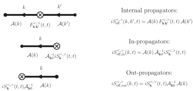
Figure 1: The Feynman rules for the flavour-coherent (effective) Wightman propagators. The propagators are composed of the spectral function ${\cal A}(k)$ (fermionic lines) and the effective 2-point vertices (circled crosses) encoding the quantum statistical information.

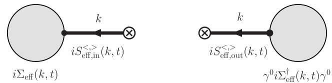
Figure 2: A diagrammatic representation of the interaction terms $I(t)$ (left) and $\gamma^{0}I^{\dagger}(t)\gamma^{0}$ (right) in the kinetic equation (23).

In figure 1 we show diagrammatic representations of the flavour-coherent cQPA propagators, which are composed of the spectral function ${\cal A}(k)$ (8) and the effective 2-point vertices $F^{<,>}_{\mathbf{k}\,\mathbf{k^{\prime}}}(t,t)$ (32) (or ${\cal A}_{\mathbf{k}0}^{-1}iS^{<,>}_{\mathbf{k}}(t,t)$ and $iS^{<,>}_{\mathbf{k}}(t,t){\cal A}_{\mathbf{k}0}^{-1}$ for in/out-propagators, respectively), encoding the quantum statistical information. In figure 2 we show generic structures of the interaction terms $I(t)$ and $I^{\dagger}(t)$ appearing in the kinetic equation (23).

These Feynman rules can be used to compute any type of Green’s function in CTP formalism, not only the self-energies appearing in (KB-) kinetic equations. For example, a perturbative contribution to full Wightman function becomes:

$$iS^{<}_{\rm pert}(k,t)= \int{\rm d}(t_{1}-t_{2})e^{ik_{0}(t_{1}-t_{2})}\int{\rm d}w_{0}{\rm d}w_{0}^{\prime}\,iS^{<}_{\mathbf{k}}(t_{1},w_{0})i\Sigma^{>}_{\mathbf{k}}(w_{0},w_{0}^{\prime})iS^{<}_{\mathbf{k}}(w_{0}^{\prime},t_{2})+\ldots$$

$$= 2\int\frac{{\rm d}k_{0}^{\prime}}{2\pi}\frac{{\rm d}^{4}p}{(2\pi)^{4}}iS^{<}_{{\rm eff}}\big{(}(k_{0}^{\prime},\mathbf{k}),p,t\big{)}i\Sigma^{>}_{\rm eff}(p,t)iS^{<}_{\rm eff}\big{(}p,(2k^{0}-k_{0}^{\prime},\mathbf{k}),t\big{)}+\ldots\,,$$ (35)

where we have again used shifts in the integration variables such as $w_{0}\to\tilde{w}_{0}=w_{0}-t$. We notice the similar convolution structure as in the case of zeroth order correlator in Eq. (19). For the corresponding local correlator we then get by $k_{0}$-integration over Eq. (35):

$$iS^{<}_{\mathbf{k},{\rm pert}}(t,t)=\int\frac{{\rm d}k_{0}}{2\pi}iS^{<}_{{\rm eff,out}}(k,t)i\Sigma^{>}_{\rm eff}(k,t)iS^{<}_{\rm eff,in}(k,t)+\ldots\,.$$ (36)

The perturbative expansion in Eqs. (35-36) is performed around the time instant $t$, i.e. the implicit local correlators $S^{<,>}_{\mathbf{k}}(t,t)$ appearing on the RHS carry the full (quantum) statistical information. Therefore Eq. (36) is actually an equation for $S^{<}_{\mathbf{k}}(t,t)$. On the other hand, by performing the perturbative expansion around the “initial” local correlators $S^{<,>}_{\mathbf{k}}(0,0)$, we find a relation

$$iS^{<}_{\rm pert}(k,t)={\cal A}_{\mathbf{k}}(t){\cal A}_{\mathbf{k}0}^{-1}iS^{<}_{\rm pert}(k,0){\cal A}_{\mathbf{k}0}^{-1}{\cal A}_{\mathbf{k}}(-t)\,,$$ (37)

where $iS^{<}_{\rm pert}(k,0)$ can be read off Eq (35) by setting $t=0$. By identifying $U_{\mathbf{k}}(t)={\cal A}_{\mathbf{k}}(y){\cal A}_{\mathbf{k}0}^{-1}$ as a quasiparticle time-evolution operator according to Eq. (15), we see that Eq. (37) corresponds to perturbative time evolution in quasiparticle interaction picture. It is well known that out-of-equilibrium perturbative time evolution suffers from secularity, and the error becomes large for $\Gamma t\gtrsim 1$ (see e.g. [31]). In contradistinction, in cQPA we do not use the perturbative expansion around initial time correlators. Instead we expand the interaction terms $I(t)$ in the kinetic equation (23) in terms of the local correlators $S^{<,>}_{\mathbf{k}}(t,t)$, and solve the resulting local time-evolution equations for $S^{<,>}_{\mathbf{k}}(t,t)$. Since the expansion is made around the time-evolved correlators, this procedure does not suffer from secular error growth. We will show this in section 6.2 below by computing iteratively the magnitude of the neglected correction terms.

5.1 Example: One-loop self-energy in Yukawa theory

As an example of the Feynman rules, we write down the effective one-loop self-energies $i\Sigma_{\rm eff}^{<,>}(k,t)$ in a Yukawa theory described by the (interaction) Lagrangian

$${\cal L}_{\rm int}=-y_{ij}\;\bar{\psi}_{i}\,\phi\,P_{L}\psi_{j}+h.c.\,,$$ (38)

where $y_{ij}$ is a complex Yukawa coupling matrix in flavour indices. The one-loop self-energy diagram(s) can be obtained for example from the two-particle irreducible (2PI) effective action [32] two-loop vacuum diagram:

$$\Gamma_{\rm 2PI}=-y_{ij}y_{lm}^{\dagger}\int_{C}{\rm d}^{4}u\,{\rm d}^{4}v\,{\rm Tr}\left[P_{L}S_{jl}(u,v)P_{R}S_{mi}(v,u)\right]\Delta(u,v)\,,$$ (39)

where sum over repeated flavour indices $i,j,l,m$ is understood, and the integration is over the Keldysh path (see e.g. [1]). $\Delta(u,v)$ denotes the scalar field (CTP) propagator. The fermion self-energy now follows by a functional differentiation:

$$\Sigma^{ab}_{ij}(u,v)= -iab\frac{\delta\Gamma_{2}[S]}{\delta S^{ba}_{ji}(v,u)}$$

$$= i\left[y_{il}^{\dagger}y_{mj}P_{R}S^{ab}_{lm}(u,v)P_{L}\Delta^{ba}(v,u)+y_{il}y_{mj}^{\dagger}P_{L}S^{ab}_{lm}(u,v)P_{R}\Delta^{ab}(u,v)\right]\,.$$ (40)

By performing a Wigner transformation, we now find for the self-energies $i\Sigma^{<,>}(k,t)$

$$i\Sigma^{<,>}_{ij}(k,t)=\int\frac{{\rm d}^{4}q}{(2\pi)^{4}}\frac{{\rm d}^{4}p}{(2\pi)^{4}}(2\pi)^{4}\delta^{4}(k-q-p)\big{[} y_{il}^{\dagger}y_{mj}P_{R}iS^{<,>}_{lm}(q,t)P_{L}i\Delta^{>,<}(-p,t)$$

$$+ y_{il}y_{mj}^{\dagger}P_{L}iS^{<,>}_{lm}(q,t)P_{R}i\Delta^{<,>}(p,t)\big{]}\,.$$ (41)

On the other hand, the effective self-energies $i\Sigma^{<,>}_{\rm eff}(k,t)$ appearing in the kinetic equations (23) (and below in Eqs. (43) and (49)) are obtained by using the cQPA Feynman rules developed in this section. By assuming that the scalar propagators $\Delta^{<,>}$ are non-coherent, we get (see Fig. 3)

$$i\Sigma^{<,>}_{{\rm eff},ij}(k,t)=\int\frac{{\rm d}^{4}q}{(2\pi)^{4}}\frac{{\rm d}^{4}q^{\prime}}{(2\pi)^{4}}\frac{{\rm d}^{4}p}{(2\pi)^{4}} (2\pi)^{4}\delta^{4}(k-q-p)$$

$$\times\big{[} y_{il}^{\dagger}y_{mj}P_{R}iS^{<,>}_{{\rm eff},lm}(q^{\prime},q,t)P_{L}i\Delta^{>,<}(-p,t)$$

$$+ y_{il}y_{mj}^{\dagger}P_{L}iS^{<,>}_{{\rm eff},lm}(q^{\prime},q,t)P_{R}i\Delta^{<,>}(p,t)\big{]}\,.$$ (42)

We notice that the 4-momentum is not formally conserved in the out-vertex of this self-energy diagram (unless $q^{\prime}=q$). However, the $q^{\prime}$-integration can always be performed trivially because of the singularity structure of $S^{<,>}_{{\rm eff}}(q^{\prime},q,t)$. This results to appropriate energy projections of the spinor structure, such that the kinematical interpretation of the (coherent) collision process remains natural. By using the explicit expressions (31-32) one can write Eq. (42) in terms of the local correlators $S^{<,>}_{\mathbf{q}}(t,t)$, and perform some of the momentum integrations. Further simplifications of Eq. (42) would require a specification of the fermionic spectral function (8) and the scalar correlators $\Delta^{<,>}(p,t)$, and are therefore model dependent.

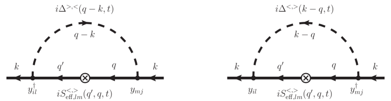
Figure 3: The Feynman diagrams contributing to the (effective) self-energies $\Sigma_{{\rm eff},ij}^{<,>}(k,t)$ at one-loop level ($i,j,l,m$ are flavour indices).

6 Kinetic equations II

In this section, we use the cQPA Feynman rules to rewrite and simplify the interaction terms in the first order kinetic equations (23) in order to obtain (local) time-evolution equations for the local correlators $\bar{S}^{<}_{\mathbf{k}}(t,t)$. In the case of vanishing dispersive self-energy $\Sigma^{h}$, we also write down the corresponding flavoured quantum Boltzmann equations for the on-shell distribution functions, given by Eq. (22). Finally, we present an estimation for the error in time evolution resulting from our approximations.

To begin, we use the results (28) and (33) with Eqs. (30) and (34) for the interaction terms in the kinetic equation (23) to get for $S^{<}$

$$\partial_{t}\bar{S}^{<}_{\mathbf{k}}(t,t)=-i\big{[}\tilde{H}_{\mathbf{k},{\rm eff}}(t),\bar{S}^{<}_{\mathbf{k}}(t,t)\big{]}^{m}-\frac{1}{2}\left(\big{\{}\tilde{\Sigma}^{>}_{\mathbf{k}}(t),\bar{S}^{<}_{\mathbf{k}}(t,t)\big{\}}^{m}-\big{\{}\tilde{\Sigma}^{<}_{\mathbf{k}}(t),\bar{S}^{>}_{\mathbf{k}}(t,t)\big{\}}^{m}\right)\,,$$ (43)

where we have defined

$$\tilde{H}_{\mathbf{k},{\rm eff}}(t)\equiv H_{\mathbf{k}0}(t)+\tilde{\Sigma}^{h}_{\mathbf{k}}(t)\,,$$ (44)

and (for all components of self-energy)

$$\tilde{\Sigma}_{\mathbf{k}}(t)\equiv\int\frac{{\rm d}k_{0}}{2\pi}\,\bar{\Sigma}_{\rm eff}(k,t){\cal A}(k){\cal A}_{\mathbf{k}0}^{-1}=\sum_{i}\bar{\Sigma}_{\rm eff}(\tilde{\omega}_{i\mathbf{k}},\mathbf{k},t)A_{i\mathbf{k}}{\cal A}_{\mathbf{k}0}^{-1}\,,$$ (45)

where we denote $\bar{\Sigma}^{h}\equiv\gamma^{0}\Sigma^{h}$ and $\bar{\Sigma}^{<,>}\equiv\gamma^{0}i\Sigma^{<,>}$ and we have used Eq. (8) for the spectral function. The generalized (anti)commutators (with respect to both Dirac and flavour indices) are defined as

$$\big{[}A,B\big{]}^{m}\equiv AB-B^{\dagger}A^{\dagger}\,,\quad\{A,B\}^{m}\equiv AB+B^{\dagger}A^{\dagger}\,.$$ (46)

We don’t need to consider the kinetic equation for $S^{>}_{\mathbf{k}}(t,t)$, because the Wightman functions are in general related by

$$S^{>}=-S^{<}-2i{\cal A}$$ (47)

and the spectral function ${\cal A}$, given by Eq. (8), is non-dynamical. The effective self-energies $\Sigma_{\rm eff}(k,t)$ are written in terms of the local correlators $\bar{S}^{<}_{\mathbf{k}}(t,t)$ (and similarly for other fields coupling to field $\psi$) using the Feynman rules of the previous section. The kinetic equation (43) is therefore local in time $t$ for arbitrary interactions, and hence an ordinary (coupled) first order differential equation in contrast to integro-differential equations with full memory integrals (see e.g. [34]). However, the kinetic equation (43) is not in general diagonal in momentum $|\mathbf{k}|$ due to (possible) self-interactions. Furthermore, if $\Sigma^{h}$ does not depend on the dynamical correlators, we find to leading order in $\Sigma^{h}$: $\tilde{\Sigma}^{h}_{\mathbf{k}}(t)=\int{\rm d}y\,\bar{\Sigma}^{h}_{\mathbf{k}}(y,t)e^{iH_{\mathbf{k}0}(t)y}$ such that $\tilde{H}_{\mathbf{k},{\rm eff}}(t)=H_{\mathbf{k},{\rm eff}}(t)$, where the adiabatic $t$-dependence is now explicitly shown. We have assumed this non-dynamical $\Sigma^{h}$ generally in the zeroth order equations in order to solve the phase-space structure of the cQPA propagators. However, in the (first order) kinetic equation (43) we can relax this assumption and consider dispersive self-energies $\Sigma^{h}$ which involve dynamical correlators and (flavour) coherence in the same footing as absorptive self-energies $\Sigma^{<,>}$.

In the case of an interaction with a thermal bath, the leading order self-energies do not depend on the dynamical correlators (thus $\Sigma_{\rm eff}(k,t)\to\Sigma(k,t)$) and they satisfy KMS relations [35] ($\beta\equiv 1/T$):

$$\Sigma^{>}(k,t)=e^{\beta k_{0}}\Sigma^{<}(k,t)\,.$$ (48)

Using the relations (47-48) in the kinetic equation (43), we then find a linear equation

$$\partial_{t}\bar{S}^{<}_{\mathbf{k}}(t,t)=-i\big{[}H_{\mathbf{k},{\rm eff}}(t),\bar{S}^{<}_{\mathbf{k}}(t,t)\big{]}^{m}-\Big{(}\big{\{}\tilde{\Gamma}_{\mathbf{k}}(t),\bar{S}^{<}_{\mathbf{k}}(t,t)\big{\}}^{m}-\int\frac{{\rm d}k_{0}}{2\pi}\,\big{\{}\bar{\Gamma}(k,t),\bar{S}^{<}_{\rm eq}(k,t)\big{\}}^{m}\Big{)}\,,$$ (49)

where $\tilde{\Gamma}_{\mathbf{k}}(t)$ is given by the analogous relation to Eq. (45) with $\bar{\Gamma}=\gamma^{0}\Gamma=(\bar{\Sigma}^{>}+\bar{\Sigma}^{<})/2$, and

$$iS^{<}_{\rm eq}(k,t)= 2f_{\rm eq}(k_{0})A(k,t)$$

$$= 2\pi\,{\rm sgn}(k_{0})f_{\rm eq}(k_{0})\delta\big{(}\mathbin{k\mkern-10.0mu\big{/}}-m_{h}(t)-i\gamma^{5}m_{a}(t)-\Sigma^{h}(k,t)\big{)}\,,$$ (50)

with $f_{\rm eq}(k_{0})=(e^{\beta k_{0}}+1)^{-1}$, is the standard quasiparticle Wightman function in (local) thermal equilibrium [33].

The structure of the kinetic equation (43) or (49) with generalized (anti)commutators is very similar to the equations of motion for the flavoured density matrix in the standard density matrix approach to flavour mixing phenomena (see e.g. ref. [8]). Indeed, the local correlator $\bar{S}^{<}_{\mathbf{k},ij}(t,t)$ is closely related to the density matrix in the basis of eigenstates $u^{*}_{i}(\mathbf{k},h)a^{\dagger}_{i\mathbf{k}}|0\rangle$ and $v_{i}(\mathbf{k},h)b^{\dagger}_{i\mathbf{k}}|0\rangle$. However, to obtain the usual equation of motion for the integrated density matrix in the flavour indices only, one would need to make a factorization ansatz in Eq. (43):

$$\bar{S}^{<}_{\mathbf{k},ij}(t,t)\sim g(\mathbf{k})\rho_{ij}(t)\,,$$ (51)

where the dependence on the momentum $\mathbf{k}$ and Dirac-indices is factorized to the function $g(\mathbf{k})$. In general, this kind of ansatz is not justified unless some stringent extra constraints are imposed. We want to emphasize that our kinetic equations (43) and (49) with the self-energy functions (45) are derived from first principles using the methods of nonequilibrium quantum field theory.

In order to solve the kinetic equation (43) for $S^{<}_{\mathbf{k}}(t,t)$, one needs to parametrize the most general spatially homogeneous local correlator $S^{<}_{\mathbf{k}}(t,t)$ in terms of eight independent matrices of (sub-)Dirac algebra, consisting of the products of $\gamma^{0}$, $\mathbf{k}\cdot\mathbf{\gamma}$ and $\gamma^{5}$. Then, using the hermiticity properties (under the Dirac and flavour indices) we obtain coupled equations of motion for $8N^{2}$ real functions of $|\mathbf{k}|$ and $t$, where $N$ is the number of flavours. We note that the equation (43) can be solved in any flavour basis, where the quasiparticle spectral function (8) is determined.

6.1 Flavoured quantum Boltzmann equations

In the limit of vanishing dispersive self-energy $\Sigma^{h}$, we can use Eq. (22) for the Wightman functions in the mass basis, where the on-shell distribution functions $f^{m<,>}_{ijh\pm}(\mathbf{k},t)$ and $f^{c<,>}_{ijh\pm}(\mathbf{k},t)$ are the dynamical variables. Using the projection operators $P_{h}$ and $\mathbin{k\mkern-10.0mu\big{/}}_{i\pm}+m_{i}$, we can then solve the distribution functions in terms of local correlators $S^{<,>}_{\mathbf{k}}(t,t)$ and use the kinetic equation (43) to obtain

$$\partial_{t}f^{m<,>}_{ijh\pm}= \mp i2\Delta\omega_{ij}f^{m<,>}_{ijh\pm}+iX^{m}_{h\pm}[f]_{ij}+{\cal C}^{m}_{h\pm}[f]_{ij}\,,$$ (52)

$$\partial_{t}f^{c<,>}_{ijh\pm}= \mp i2\bar{\omega}_{ij}f^{c<,>}_{ijh\pm}+iX^{c}_{h\pm}[f]_{ij}+{\cal C}^{c}_{h\pm}[f]_{ij}\,,$$ (53)

where $X^{m,c}_{h\pm}[f]$ involve terms proportional to mass and mixing gradients: $\partial_{t}m_{i}/\omega_{i}^{2}$ and $\Xi^{\prime\pm}\equiv i\big{(}V\partial_{t}V^{\dagger}\pm U\partial_{t}U^{\dagger}\big{)}/2$, and ${\cal C}^{m,c}_{h\pm}[f]$ are the collision integrals. From these flavoured quantum Boltzmann equations (52-53) we can directly see that to zeroth order the on-shell functions $f^{m<,>}_{ijh\pm}$ and $f^{c<,>}_{ijh\pm}$ are oscillating at frequencies $\Delta\omega_{ij}$ and $\bar{\omega}_{ij}$, respectively. We present the full expressions of $X^{x}_{h\pm}$ and ${\cal C}^{x}_{h\pm}$ in [7] for a general $N\times N$-mixing scenario and a general Dirac decomposition of spatially homogeneous self-energies.

6.2 Estimation of error in time evolution

In order to obtain the local evolution equation (43) for $S^{<,>}_{\mathbf{k}}(t,t)$ we have extensively used the zeroth order equations (14) and (17) inside the interaction terms $I(t)$ of the full kinetic equation (23). In this section we estimate the magnitude of the error resulting from this approximation.

First, we notice that the convolutions $I(t)$ can be written in Wigner representation as

$$I_{\rm full}(t)\equiv \int{\rm d}t^{\prime}\,\Sigma_{\mathbf{k}}(t,t^{\prime})S^{<,>}_{\mathbf{k}}(t^{\prime},t)$$

$$= \int\frac{{\rm d}k_{0}}{2\pi}e^{-i\Diamond}\{\Sigma(k,t)\}\{S^{<,>}(k,t)\}$$

$$= \int\frac{{\rm d}k_{0}}{2\pi}\sum_{n=0}^{\infty}\frac{1}{n!}\Big{(}\frac{i}{2}\Big{)}^{n}\partial_{t}^{n}\Big{(}\big{(}\partial_{k_{0}}^{n}\Sigma(k,t))\,S^{<,>}(k,t)\Big{)}\,,$$ (54)

where the $\Diamond$-operator is defined as

$$\Diamond\{f\}\{g\}=\frac{1}{2}\big{(}\partial_{t}f\,\partial_{k_{0}}g-\partial_{k_{0}}f\,\partial_{t}g\big{)}\,.$$ (55)

Next, by using Eqs. (19) and (23) or alternatively KB-equation (2) in Wigner representation, we can parametrically estimate the time-derivatives appearing in Eq. (54) as

$$\partial_{t}S(k,t)\sim k_{0}S(k,t)+\epsilon\,k_{0}S(k,t)\,,$$

$$\partial_{t}\Sigma(k,t)\sim k_{0}\Sigma(k,t)+\epsilon\,k_{0}\Sigma(k,t)\,,$$ (56)

with

$$\epsilon\sim\Big{\{}\frac{\partial_{t}m}{k_{0}^{2}},\frac{\Sigma(k,t)}{k_{0}}\Big{\}}\,.$$ (57)

The zeroth ($\epsilon$-)order terms in the RHS of Eqs. (56) arise from the commutators of the (coherent) correlators $S^{<,>}$ with the Hamiltonian $H_{\mathbf{k}0}$ in Eq. (23), and accordingly for the self-energies involving coherent correlators. We may further estimate $\partial_{k_{0}}\Sigma(k,t)\sim\Sigma(k,t)/k_{0}$ to get

$$\partial_{t}\Big{(}\big{(}\partial_{k_{0}}\Sigma(k,t))\,S^{<,>}(k,t)\Big{)}\sim\Sigma(k,t)S(k,t)+\epsilon\,\Sigma(k,t)S(k,t)\,,$$ (58)

and furthermore by using Eq. (54)

$$I_{\rm full}(t)\sim\int\frac{{\rm d}k_{0}}{2\pi}\Big{[}\Sigma_{\rm eff}(k,t)S^{<,>}_{\rm eff,in}(k,t)+\sum_{n=1}^{\infty}\epsilon^{n}\,\Sigma(k,t)S(k,t)\Big{]}\,,$$ (59)

where we have noticed that all zeroth order terms have been accounted for in the effective propagators and self-energies. We see that the corrections to the leading order terms included in kinetic equations (43) are suppressed by powers of $\partial_{t}m/k_{0}^{2}$ and $\Sigma/k_{0}$. Therefore, we conclude that in the case of weak interactions and small gradients of the background field ($\epsilon\ll 1$) the error of expanding the interaction terms $I(t)$ in terms of local correlators $S^{<,>}_{\mathbf{k}}(t,t)$ by using the cQPA Feynman rules is small for any instant of time $t$. Consequently, the error of time evolution is not growing as $\Gamma t$ as in the case of secular evolution, but rather, our error is that the scattering rate $\Gamma$ (and the thermalization time $\sim 1/\Gamma$) is misevaluated by a small correction: $\Gamma_{\rm full}\approx(1+\epsilon)\Gamma$.

7 Conclusions and outlook

In this work we have presented a flavour-covariant formulation of the coherent propagators and Feynman rules for flavour-mixing fermionic fields in spatially homogeneous and isotropic systems. Our formalism is based on the coherent quasiparticle approximation (cQPA) [1, 2, 3, 4, 5, 6, 7], where nonlocal coherence information is encoded in new spectral solutions at off-shell momenta. In addition to more simplified covariant formulation, we have generalized our previous work [7] to the case of nonzero dispersive self-energy, which leads to a broader range of applications.

The new formulation is based on the two-time representation of the correlators and it immediately reveals the composite nature of the cQPA Wightman function as a product of two spectral functions and a local correlator, interpreted as an effective two-point interaction vertex, which contains all quantum statistical and coherence information (see Eqs. (18-19) and (31)). This derived form can be viewed as a generalization of the well known Kadanoff-Baym ansatz to coherent systems. In section 5, we have derived the cQPA Feynman rules involving the flavour-coherent (composite) propagators, presented in Fig. 1. These rules are designed for computing the interaction terms of the Kadanoff-Baym equations (23) in momentum space in terms of the local correlators $S^{<,>}_{\mathbf{k}}(t,t)$, and they can in principle be applied to arbitrarily complex self-energies involving flavour-coherent propagators inside the loop-integrals.

We have used the cQPA Feynman rules to derive flavoured kinetic equations (43) for the local correlators $S^{<,>}_{\mathbf{k}}(t,t)$ in the presence of dispersive and absorptive interactions. These equations are local in time-variable $t$, and they can as well be rewritten as flavoured quantum Boltzmann equations for the (enlarged) set of on-shell distribution functions $f(\mathbf{k},t)$. The structure of Eqs. (43) is very intuitive, consisting of the generalized commutators and anticommutators in both flavour and Dirac indices. They are reminiscent of the equations of motion for the (flavoured) density matrix used e.g. in refs. [8]. We want to emphasize that in our approach all the interaction terms, given by Eq. (45), are derived from first principles of nonequilibrium quantum field theory by consistent approximations using the cQPA scheme. We have further shown that the corrections to our results are (parametrically) suppressed by the powers of $\partial_{t}m/k_{0}^{2}$ and $\Sigma(k,t)/k_{0}$.

In the present work we have extended the cQPA scheme to include dispersive self-energy corrections, which allows the treatment of quasi-excitations in plasmas. The natural applications of the formalism include for example neutrino flavour oscillations in the early universe [36] and electroweak baryogenesis, where the formalism needs to be generalized to the case of a stationary planar symmetry, as discussed in ref. [1]. Another interesting application to our formalism is a consistent approach to resonant leptogenesis, where the flavour coherence effects of the singlet neutrinos are expected to play an important role in the dynamics. In the regime of nearly degenerate neutrino masses, the formalism should be extended to include appropriate finite width corrections for the propagators.

References

• [1] M. Herranen, K. Kainulainen and P. M. Rahkila, Towards a kinetic theory for fermions with quantum coherence, Nucl. Phys.  B 810 (2009) 389 [arXiv:0807.1415 [hep-ph]].
• [2] M. Herranen, K. Kainulainen and P. M. Rahkila, Quantum kinetic theory for fermions in temporally varying backgrounds, JHEP 0809 (2008) 032 [arXiv:0807.1435 [hep-ph]].
• [3] M. Herranen, K. Kainulainen and P. M. Rahkila, Kinetic theory for scalar fields with nonlocal quantum coherence, JHEP 0905 (2009) 119 [arXiv:0812.4029v2 [hep-ph]].
• [4] M. Herranen, K. Kainulainen and P. M. Rahkila, Coherent quasiparticle approximation cQPA and nonlocal coherence, J. Phys. Conf. Ser.  220 (2010) 012007 [arXiv:0912.2490 [hep-ph]].
• [5] M. Herranen, Quantum kinetic theory with nonlocal coherence, PhD Thesis, University of Jyväskylä Res. Rep. 3/2009 [arXiv:0906.3136 [hep-ph]].
• [6] M. Herranen, K. Kainulainen and P. M. Rahkila, Coherent quantum Boltzmann equations from cQPA, JHEP 1012 (2010) 072 [arXiv:1006.1929 [hep-ph]].
• [7] C. Fidler, M. Herranen, K. Kainulainen and P. M. Rahkila, Flavoured quantum Boltzmann equations from cQPA, arXiv:1108.2309 [hep-ph].
• [8] R. Barbieri and A. Dolgov, Bounds On Sterile-Neutrinos From Nucleosynthesis, Phys. Lett. B 237 (1990) 440; Neutrino oscillations in the early universe, Nucl. Phys. B 349 (1991) 743;
K. Kainulainen, Light Singlet Neutrinos And The Primordial Nucleosynthesis, Phys. Lett. B 244 (1990) 191;
K. Enqvist, K. Kainulainen and J. Maalampi, Resonant Neutrino Transitions And Nucleosynthesis, Phys. Lett. B 249, 531 (1990); Refraction And Oscillations Of Neutrinos In The Early Universe, Nucl. Phys. B 349 (1991) 754;
K. Enqvist, K. Kainulainen and M. J. Thomson, Stringent cosmological bounds on inert neutrino mixing, Nucl. Phys. B 373 (1992) 498.
• [9] D. Boyanovsky, C. M. Ho, Charged lepton mixing and oscillations from neutrino mixing in the early universe, Astropart. Phys.  27 (2007) 99-112;
C. M. Ho, D. Boyanovsky, H. J. de Vega, Neutrino oscillations in the early universe: A Real time formulation, Phys. Rev.  D72 (2005) 085016.
• [10] V. A. Kuzmin, V. A. Rubakov and M. E. Shaposhnikov, On The Anomalous Electroweak Baryon Number Nonconservation In The Early Universe, Phys. Lett.  B 155 (1985) 36;
A. G. Cohen, D. B. Kaplan and A. E. Nelson, Progress in electroweak baryogenesis, Ann. Rev. Nucl. Part. Sci.  43 (1993) 27 [arXiv:hep-ph/9302210];
V.A. Rubakov and M.E. Shaposhnikov, Electroweak baryon number non-conservation in the early universe and in high-energy collisions, Usp. Fiz. Nauk 166 (1996) 493, Phys. Usp. 39 (1996) 461 [hep-ph/9603208].
• [11] M. Joyce, T. Prokopec and N. Turok, Nonlocal electroweak baryogenesis. Part 2: The Classical regime, Phys. Rev. D 53, 2958 (1996) [hep-ph/9410282]; Electroweak baryogenesis from a classical force, Phys. Rev. Lett.  75, 1695 (1995), [Erratum-ibid.  75, 3375 (1995)] [hep-ph/9408339]; Nonlocal electroweak baryogenesis. Part 1: Thin wall regime, Phys. Rev. D 53, 2930 (1996).
• [12] J. M. Cline, M. Joyce and K. Kainulainen, Supersymmetric electroweak baryogenesis, JHEP 0007 (2000) 018 [hep-ph/0006119]; Supersymmetric electroweak baryogenesis in the WKB approximation, Phys. Lett. B 417 (1998) 79, [Erratum-ibid. B 448 (1999) 321] [hep-ph/9708393];
J. M. Cline and K. Kainulainen, A new source for electroweak baryogenesis in the MSSM, Phys. Rev. Lett.  85 (2000) 5519 [hep-ph/0002272].
• [13] K. Kainulainen, T. Prokopec, M. G. Schmidt and S. Weinstock, First principle derivation of semiclassical force for electroweak baryogenesis, JHEP 0106, 031 (2001) [hep-ph/0105295]; Semiclassical force for electroweak baryogenesis: Three-dimensional derivation, Phys. Rev. D66 (2002) 043502 [hep-ph/0202177]; Quantum Boltzmann equations for electroweak baryogenesis including gauge fields, [hep-ph/0201293].
• [14] T. Prokopec, M. G. Schmidt and S. Weinstock, Transport equations for chiral fermions to order h bar and electroweak baryogenesis. Part 1., Annals Phys.  314 (2004) 208 [hep-ph/0312110]; Transport equations for chiral fermions to order h-bar and electroweak baryogenesis. Part II., Annals Phys.  314 (2004) 267 [hep-ph/0406140].
• [15] T. Konstandin, T. Prokopec and M. G. Schmidt, Kinetic description of fermion flavour mixing and CP-violating sources for baryogenesis, Nucl. Phys.  B 716 (2005) 373 [arXiv:hep-ph/0410135];
T. Konstandin, T. Prokopec, M. G. Schmidt and M. Seco, MSSM electroweak baryogenesis and flavour mixing in transport equations, Nucl. Phys.  B 738 (2006) 1 [arXiv:hep-ph/0505103].
• [16] V. Cirigliano, C. Lee, M. J. Ramsey-Musolf and S. Tulin, flavoured Quantum Boltzmann Equations, Phys. Rev.  D 81 (2010) 103503 [arXiv:0912.3523 [hep-ph]];
V. Cirigliano, C. Lee and S. Tulin, Resonant flavour Oscillations in Electroweak Baryogenesis, arXiv:1106.0747 [hep-ph].
• [17] B. Garbrecht, T. Prokopec and M. G. Schmidt, Coherent baryogenesis, Phys. Rev. Lett.  92 (2004) 061303 [arXiv:hep-ph/0304088]; SO(10) - GUT coherent baryogenesis, Nucl. Phys.  B 736 (2006) 133 [arXiv:hep-ph/0509190].
• [18] M. Fukugita and T. Yanagida, Baryogenesis Without Grand Unification, Phys. Lett.  B 174 (1986) 45.
• [19] A. Pilaftsis and T. E. J. Underwood, Resonant leptogenesis, Nucl. Phys.  B 692 (2004) 303 [arXiv:hep-ph/0309342]; Electroweak-scale resonant leptogenesis, Phys. Rev.  D 72 (2005) 113001 [arXiv:hep-ph/0506107].
• [20] A. Abada, S. Davidson, F. X. Josse-Michaux, M. Losada and A. Riotto, Flavour Issues in Leptogenesis, JCAP 0604 (2006) 004 [arXiv:hep-ph/0601083];
E. Nardi, Y. Nir, E. Roulet and J. Racker, The importance of flavour in leptogenesis, JHEP 0601 (2006) 164 [arXiv:hep-ph/0601084];
M. Garny, A. Hohenegger, A. Kartavtsev and M. Lindner, Systematic approach to leptogenesis in nonequilibrium QFT: vertex contribution to the CP-violating parameter, Phys. Rev.  D 80 (2009) 125027 [arXiv:0909.1559 [hep-ph]]; Systematic approach to leptogenesis in nonequilibrium QFT: self-energy contribution to the CP-violating parameter, Phys. Rev.  D 81 (2010) 085027 [arXiv:0911.4122 [hep-ph]];
M. Beneke, B. Garbrecht, M. Herranen and P. Schwaller, Finite Number Density Corrections to Leptogenesis, Nucl. Phys.  B 838 (2010) 1 [arXiv:1002.1326 [hep-ph]];
M. Beneke, B. Garbrecht, C. Fidler, M. Herranen and P. Schwaller, Flavoured Leptogenesis in the CTP Formalism, Nucl. Phys.  B 843 (2011) 177 [arXiv:1007.4783 [hep-ph]];
A. Anisimov, D. Besak and D. Bodeker, Thermal production of relativistic Majorana neutrinos: Strong enhancement by multiple soft scattering, JCAP 1103 (2011) 042 [arXiv:1012.3784 [hep-ph]].
• [21] A. Anisimov, W. Buchmuller, M. Drewes and S. Mendizabal, Leptogenesis from Quantum Interference in a Thermal Bath, Phys. Rev. Lett.  104 (2010) 121102 [arXiv:1001.3856 [hep-ph]]; Quantum Leptogenesis I, Annals Phys.  326 (2011) 1998 [arXiv:1012.5821 [hep-ph]].
• [22] J. H. Traschen and R. H. Brandenberger, Particle production during out-of-equilibrium phase transitions, Phys. Rev. D 42 (1990) 2491;
Y. Shtanov, J. H. Traschen and R. H. Brandenberger, Universe reheating after inflation, Phys. Rev. D51 (1995) 5438 [arXiv:hep-ph/9407247];
J. Berges and J. Serreau, Parametric resonance in quantum field theory, Phys. Rev. Lett.  91 (2003) 111601 [arXiv:hep-ph/0208070];
J. Berges, J. Pruschke and A. Rothkopf, Instability-induced fermion production in quantum field theory, Phys. Rev.  D 80 (2009) 023522 [arXiv:0904.3073 [hep-ph]].
• [23] J. F. Koksma, T. Prokopec and M. G. Schmidt, Decoherence in an Interacting Quantum Field Theory: The Vacuum Case, Phys. Rev.  D 81 (2010) 065030 [arXiv:0910.5733 [hep-th]]; Entropy and Correlators in Quantum Field Theory, Annals Phys.  325 (2010) 1277 [arXiv:1002.0749 [hep-th]]; Decoherence in an Interacting Quantum Field Theory: Thermal Case, Phys. Rev.  D 83 (2011) 085011 [arXiv:1102.4713 [hep-th]];
A. Giraud and J. Serreau, Decoherence and thermalization of a pure quantum state in quantum field theory, Phys. Rev. Lett.  104 (2010) 230405 [arXiv:0910.2570 [hep-ph]];
F. Gautier and J. Serreau, Quantum properties of a non-Gaussian state in the large-N approximation, Phys. Rev.  D 83 (2011) 125004 [arXiv:1104.0421 [quant-ph]].
• [24] J. S. Schwinger, Brownian motion of a quantum oscillator, J. Math. Phys.  2 (1961) 407;
L. V. Keldysh, Diagram technique for nonequilibrium processes, Zh. Eksp. Teor. Fiz.  47 (1964) 1515 [Sov. Phys. JETP 20 (1965) 1018].
• [25] P. Danielewicz, Quantum Theory Of Nonequilibrium Processes. 1, Annals Phys. 152 (1984) 239;
S. Mrowczynski and U. W. Heinz, Towards a relativistic transport theory of nuclear matter, Annals Phys. 229 (1994) 1.
• [26] E. Calzetta and B. L. Hu, Nonequilibrium Quantum Field Theory, Cambridge, UK: Univ. Pr. (2008) 535 p.
• [27] C. Greiner and S. Leupold, Stochastic interpretation of Kadanoff-Baym equations and their relation to Langevin processes, Annals Phys.  270 (1998) 328 [arXiv:hep-ph/9802312].
• [28] A. Anisimov, W. Buchmuller, M. Drewes and S. Mendizabal, Nonequilibrium Dynamics of Scalar Fields in a Thermal Bath, Annals Phys.  324 (2009) 1234 [arXiv:0812.1934 [hep-th]].
• [29] L. Kadanoff and G. Baym, Quantum Statistical Mechanics, Benjamin, New York (1962).
• [30] M. Le Bellac, Thermal Field Theory, Cambridge University Press, 2000.
• [31] J. Berges, Introduction to nonequilibrium quantum field theory, AIP Conf. Proc.  739 (2005) 3 [arXiv:hep-ph/0409233].
• [32] J. M. Luttinger and J. C. Ward, Ground state energy of a many fermion system. 2, Phys. Rev.  118 (1960) 1417:
J. M. Cornwall, R. Jackiw and E. Tomboulis, Effective Action For Composite Operators, Phys. Rev.  D 10 (1974) 2428;
K. c. Chou, Z. b. Su, B. l. Hao and L. Yu, Equilibrium And Nonequilibrium Formalisms Made Unified, Phys. Rept.  118 (1985) 1;
E. Calzetta and B. L. Hu, Nonequilibrium Quantum Fields: Closed Time Path Effective Action, Wigner Function and Boltzmann Equation, Phys. Rev.  D 37 (1988) 2878.
• [33] H. A. Weldon, Dynamical holes in the quark-gluon plasma, Phys. Rev.  D 40 (1989) 2410;
Particles and holes, Physica A 158 (1989) 169.
• [34] J. Berges and J. Cox, Thermalization of quantum fields from time-reversal invariant evolution equations, Phys. Lett. B 517 (2001) 369 [arXiv:hep-ph/0006160];
J. Berges, Controlled nonperturbative dynamics of quantum fields out of equilibrium, Nucl. Phys. A 699 (2002) 847 [arXiv:hep-ph/0105311];
G. Aarts, D. Ahrensmeier, R. Baier, J. Berges and J. Serreau, Far-from-equilibrium dynamics with broken symmetries from the 2PI-1/N expansion, Phys. Rev. D 66 (2002) 045008 [arXiv:hep-ph/0201308];
J. Berges, S. Borsanyi and J. Serreau, Thermalization of fermionic quantum fields, Nucl. Phys. B 660 (2003) 51 [arXiv:hep-ph/0212404].
• [35] R. Kubo, Statistical Mechanical Theory Of Irreversible Processes. I, J. Phys. Soc. Jap.  12 (1957) 570;
R. Kubo, M. Yokota and S. Nakajima, Statistical Mechanical Theory Of Irreversible Processes. II, J. Phys. Soc. Jap.  12 (1957) 1203;
P. C. Martin and J. S. Schwinger, Theory of many particle systems. I, Phys. Rev.  115 (1959) 1342.
• [36] J. Ilmavirta, K. Kainulainen and P. M. Rahkila, Neutrino transport in coherent quasiparticle approximation, in preparation.