Normal persistent currents in proximity-effect bilayers

Abstract

We calculate the contribution of superconducting fluctuations to the mesoscopic persistent current of an ensemble of rings, each made of a superconducting layer in contact with a normal one, in the Cooper limit. The superconducting transition temperature of the bilayer decays very quickly with the increase of the relative width of the normal layer. In contrast, when the Thouless energy is larger than the temperature then the suppression of the persistent current with the increase of this relative width is much slower than that of the transition temperature. This effect is similar to that predicted for magnetic impurities, although the proximity effect considered here results in pair-weakening as opposed to pair-breaking.

I Introduction

The average persistent current BUTTIKER ; BOOK of a large number of mesoscopic metallic rings can be used to deduce the sign and the magnitude of electron-electron interactions in the metal forming the rings. The size of the average current is expected to increase with the strength of the interactions, and its sign reflects the nature of the interactions: the magnetic response at low flux is paramagnetic (diamagnetic) when the electronic interactions are repulsive (attractive).AEEPL ; AEPRL For a large ensemble of rings, the current is expected to be periodic in the magnetic flux, with the period corresponding to one half of the flux quantum, $h/2e$. The theoretical analysis of Refs. AEEPL, and AEPRL, was motivated in part by early measurements of the average persistent current in an array of $10^{6}$ copper rings, LDDB whose sign and magnitude could not be accounted for by noninteracting electrons alone and therefore should be affected by electronic interactions. These experiments confirmed the above periodicity, also suggesting that the average magnetic response is induced by interactions. AEEPL ; AEPRL Similar results were later observed on an array of $10^{5}$ GaAs rings reulet and on an array of $10^{5}$ silver rings. DBRBM In contrast, measurements on single ringswebb91 ; 10 ; 11 ; Moler showed the $h/e$ periodicity. In an array of 30 gold ringsJMKW both the $h/2e$ and the $h/e$ harmonics were observed. In this paper the authors were unable to say whether the $h/2e$ signal was the second harmonic of the typical contribution or the first harmonic of an average contribution. Overall, the sign of the $h/2e$ harmonic measured on metallic rings seems to indicate that the low-flux response is diamagnetic, DBRBM ; JMKW implying attractive interactions. Recently, Bleszynski-Jayich et al.JGEH found that the average current in aluminum rings, subject to high magnetic fields, is negligible, but typical mesoscopic fluctuations remain almost unaffected. It seems that these latter experiments can be explained within the framework of noninteracting electrons. EG ; HAMUTAL3

Interestingly enough, it turned out that the bona fide values of the attractive interactions required to explain the persistent-current data of the copper LDDB ensemble for example, would have implied that this metal is superconducting at measurable temperatures, of the order of 1mK. In fact, early experiments on the magnetic response GD0 and on the thermal conductivityGD2 of proximity-effect systems, whose normal parts were copper and silver, also indicated a minute attractive interaction in these metals.GD1 However, these early measurements allowed a broad range for the magnitude of this interaction, and therefore did not open a discussion of the reasons for the absence of superconductivity in experiments on these metals. The latter puzzle became obvious only after the measurements of the persistent current on copper, which requires a transition temperature of 1mk. Superconductivity has not been detected also in gold and silver, and this fact has remained unexplained for many years. A possible explanation for this apparent puzzle HELENE was offered in Refs.  HAMUTAL1, and  HAMUTAL2, , which argued (for the first time) that the existence of (seemingly unavoidableBIRGE ) tiny amounts of magnetic impurities may detrimentally affect superconductivity in such metals, reducing their transition temperatures to undetectable, even zero, values, while leaving the persistent current almost unharmed. This stems from the disparity of the energy scales determining the renormalized electronic interaction pertaining to each phenomenon. The interaction-induced persistent current is proportional to the renormalized interaction on the scale of the Thouless energy, $E_{c}=\hbar D/L^{2}$ (where $D$ is the diffusion coefficient and $L$ is the circumference of the ring). Superconductivity is lost, however, when the spin-flip rate of the magnetic impurities, $\hbar/\tau_{s}$ (in units of energy), becomes comparable to the bare transition temperature of the material (in the absence of any pair-breaking or pair-weakening agents), $T^{S}_{c0}$. In other words, the actual superconducting transition temperature $T^{S}_{c}$ is determined by the renormalized interaction, on the scale of $\max[T^{S}_{c0},\hbar/\tau_{s}]$. It follows that a concentration of magnetic impurities such that

$$k_{B}T^{S}_{c0}\lesssim\hbar/\tau_{s}\lesssim E_{c}\ ,$$ (1)

will hardly affect the magnitude of the persistent current, concomitantly suppressing the superconducting transition temperature (below we often use units in which $\hbar=k_{\rm B}=1$). Indeed, detailed analysis HAMUTAL2 of the persistent current data reported in Refs. LDDB, and DBRBM, led to the conclusion that $T^{S}_{c0}$ of copper (gold) is in the mK (a fraction of mK) range.

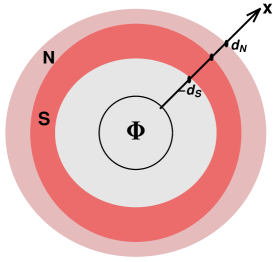
Figure 1: (color online) Proximity-effect ring in which the width of the strong (weak) superconductor is $d_{S}$ ($d_{N}$), threaded by a magnetic flux $\Phi$ (measured in units of the flux quantum).

This theoretical picture can be tested, for instance, by investigating rings made of known low-superconducting-transition-temperature materials, in which a controlled concentration of pair breakers have been added.JGEH It has also been noted that the magnetic flux itself acts as a pair breaker, causing a periodic decrease of the transition temperature but a lesser decrease in the persistent current. oreg It is interesting to check whether there exist other situations where the superconducting transition temperature is lowered by some pair-breaking or pair-weakening mechanism, but the (superconducting fluctuation-induced) persistent current remains large far above this transition temperature. In the present paper we consider this question for superconducting-normal ($SN$) bilayers, e.g. made of Al and Cu.HELENE Bilayers made of Al and Ag might even be better, as they avoid magnetic impurities. The ‘normal’ metal could also be a weaker superconductor, with a lower transition temperature. The proximity effect is known to cause a decrease of the transition temperature of the bilayer with the relative thickness of the $S$ layer,DEGENNES ; ANI and it is interesting to find out what happens to the persistent current, which is induced by superconducting fluctuations. This possibility is in particular intriguing: unlike the magnetic impurities, the proximity effect is not a bona fide pair-breaker, since time-reversal invariance is not broken by it. The proximity effect just leads to pair-weakening, by ‘diluting’ the superconducting fraction. FULDE

Here we present a calculation of the disorder-averaged persistent current averaged over an ensemble of bilayer rings, each having the geometry depicted in Fig. 1. These rings consist of two adjacent metallic rings, with different transition temperatures. The area inside the rings is penetrated by a magnetic flux $\Phi$, which is measured in units of the flux quantum $hc/e$. Below we use the subscript $S$ for quantities characterizing the layer with the higher transition temperature, and the subscript $N$ for the quantities belonging to the other one, which may or may not be a superconductor. For simplicity, we confine our calculation to bilayers in the Cooper limit: DEGENNES this limit is reached when the width of each of the layers, $d_{S}$ or $d_{N}$, is much smaller than the respective coherence length. COM2 Our aim is to explore the possibility to deduce the scale of the renormalized electronic interaction by analyzing concomitantly the superconducting transition temperature and the (superconducting) fluctuation-induced average persistent current. In other words, we examine the persistent current as a function of the $N-$slab relative thickness, and find parameter regimes where it is affected much less than the transition temperature.

Since pair breakers, notably magnetic impurities, seem to be ubiquitous in several of the metals used in the persistent-current measurements, it is interesting to investigate their effect in a proximity-effect configuration. For instance, it is plausible that in Al/Cu rings, the copper (the $N-$slab in our notations) may well include a tiny amount of magnetic impurities. We therefore include scattering off such impurities in our expressions.

The transition temperature of an $SN$ proximity bilayer in the the Cooper limit is knownDEGENNES ; ANI to be determined by the effective (dimensionless) electronic coupling, $\lambda_{NS}$, which is the weighted sum of the effective couplings of the separate slabs, $\lambda_{S}$ (which is positive, since the $S-$slab is superconducting) and $\lambda_{N}$ (which may take both signs):

$$\lambda_{NS}=p_{N}\lambda_{N}+p_{S}\lambda_{S}\ ,$$ (2)

with

$$p_{N(S)}=d_{N(S)}\widetilde{\cal N}_{N(S)}/\widetilde{\cal N}_{\rm eff}\ ,$$ (3)

where $\widetilde{\cal N}_{N(S)}$ denotes the density of states at the Fermi energy per unit length of the normal (superconducting) layer, and

$$\widetilde{\cal N}_{\rm eff}=\widetilde{\cal N}_{N}d_{N}+\widetilde{\cal N}_{S}d_{S}\ .$$ (4)

The mean-field transition temperature, $T_{c0}^{NS}$, of the bilayer (without magnetic impurities) is then given by DEGENNES ; ANI

$$\frac{1}{\lambda_{NS}}=\Psi\Bigl{(}\frac{1}{2}+\frac{\omega_{D}}{2\pi T_{c0}^{NS}}\Bigr{)}-\Psi\Bigl{(}\frac{1}{2}\Bigr{)}\ ,$$ (5)

where $\Psi$ is the digamma function whose asymptotic expansion, valid for large arguments, is given by

$$\lim_{z\to\infty}\Psi(z)\to\ln z\ .$$ (6)

The Debye frequency $\omega_{D}$ in Eq. (5) (assumed to be identical for both slabs) marks the upper cutoff on the effective interactions. The result (5) is obtained assuming that the two layers are in a good electrical contact. (The effect of a barrier between the two layers has been considered by McMillan. MAC ) In the limit $\omega_{D}\gg T^{NS}_{c0}$ one may use Eq. (6) to obtain

$$\ln\frac{T^{NS}_{c0}}{T^{S}_{c0}}=-\Bigl{(}1-\frac{\lambda_{N}}{\lambda_{S}}\Bigr{)}\frac{p_{N}}{\lambda_{N}p_{N}+\lambda_{S}p_{S}}\ ,$$ (7)

where $T^{S}_{c0}$ is the bulk transition temperature of the clean $S-$slab. When the $N-$ slab is also superconducting (i.e. $\lambda_{N}>0$), $T^{NS}_{c0}$ remains finite for all $p_{N}$ (although quite small for large $p_{N}$ and small $\lambda_{N}$). However, when $\lambda_{N}\leq 0$, the transition temperature of the bilayer $T^{NS}_{c0}$ approaches zero at a quantum critical point, $p_{N}=1/(1-\lambda_{N}/\lambda_{S})$. The approach is exponential, with zero slope (see Fig. 2). In practice, $T^{NS}_{c0}$ becomes very small for $p_{N}\gtrsim 1/2$. In some sense, this inequality replaces the left hand side of Eq. (1). As we show below, the persistent current remains rather large even in this regime.

The effect of genuine pair-breaking mechanisms on the transition temperature was considered a long time ago. The seminal paper of Abrikosov and Gorkov AG found that the transition temperature $T^{S}_{c0}$ is reduced by magnetic impurities to $T^{S}_{c}$,

$$\ln\frac{T^{S}_{c}}{T^{S}_{c0}}=\Psi\Bigl{(}\frac{1}{2}\Bigr{)}-\Psi\Bigl{(}\frac{1}{2}+\frac{sT^{S}_{c0}}{T^{S}_{c}}\Bigr{)}\ ,$$ (8)

where $s=1/(2\pi T^{S}_{c0}\tau_{s})$. This expression is shown in the inset in Fig. 2. Unlike $T^{NS}_{c0}$, $T^{S}_{c}$ approaches zero at $s=\exp[\Psi(1/2)]=1/(4\gamma_{E})\approx 0.140365$ (namely at $\hbar/\tau_{s}\sim 0.9T^{S}_{c0}$), with a finite slope. Here, $\gamma_{E}$ is the Euler constant. This difference in slope between the two mechanisms probably reflects the difference between pair-weakening and pair-breaking. FULDE

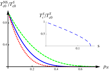
Figure 2: (color online) The transition temperature of a proximity-effect sandwich in the Cooper limit [Eq. (7)] as a function of the weighed width of the normal layer for $\lambda_{N}=0,~{}0.05$, and $-0.05$ (solid, dashed, and dotted curve, respectively). In all curves $\lambda_{S}=0.17$. The inset depicts the Abrikosov-Gorkov expression, Eq. (8), for the reduction of the transition temperature by pair breakers.

In a complete analogy with Eq. (8), a small amount of pair-breaking impurities in the $N-$slab lowers the transition temperature of the sandwich from $T_{c0}^{NS}$ to $T_{c}^{NS}$, given by ANI

$$\frac{1}{\lambda_{NS}} =\Psi\Bigl{(}\frac{1}{2}+\frac{\omega_{D}}{2\pi T_{c}^{NS}}\Bigr{)}-\Psi\Bigl{(}\frac{1}{2}+\frac{p_{N}}{2\pi T^{NS}_{c}\tau_{s}}\Bigr{)}\ ,$$ (9)

generalizing Eq. (5).

The rest of this paper describes the calculation of the average persistent current, pertaining to a large ensemble of bilayers. Section II outlines the derivation of the effective Ginzburg-Landau theory for this case, with some technical details given in Appendix A. Some quantitative results are presented in Sec. III. Since the fluctuations are calculated within the high-temperature Gaussian approximation, which is valid only above the Ginzburg critical regime, Sec. IV presents a critical discussion of this regime. That section also contains our conclusions.

II The persistent current of a proximity-effect sandwich

Here we present a microscopic derivation of the free energy which determines the superconducting fluctuations. The Hamiltonian of the bilayer is similar to that used in Refs. HAMUTAL1, and HAMUTAL2, ,

$${\cal H}=\int d{\bf r}{\cal H}({\bf r})\ ,$$ (10)

with

$${\cal H}({\bf r}) =\sum_{\sigma\sigma^{\prime}}\psi_{\sigma}^{\dagger}({\bf r}){\cal H}^{(0)}_{\sigma\sigma^{\prime}}({\bf r})\psi_{\sigma^{\prime}}({\bf r})$$

$$-V({\bf r})\psi^{\dagger}_{\uparrow}({\bf r})\psi^{\dagger}_{\downarrow}({\bf r})\psi_{\downarrow}({\bf r})\psi_{\uparrow}({\bf r})\ ,$$ (11)

where $\psi_{\sigma}^{\dagger}({\bf r})$ creates an electron with spin $\sigma$ at ${\bf r}$. The interaction $V({\bf r})$ depends on the spatial coordinate $x$ (see Fig. 1),

$$V(x) =\lambda_{S}/{\cal N}_{S}\ ,\ \ \ -d_{S}\leq x\leq 0$$

$$V(x) =\lambda_{N}/{\cal N}_{N}\ ,\ \ \ 0\leq x\leq d_{N}\ .$$ (12)

(Note that here the ${\cal N}$’s are the densities of states per unit volume of the two layers.) The single-particle part of the Hamiltonian (11) reads

$${\cal H}^{(0)}_{\sigma\sigma^{\prime}}({\bf r})=\delta_{\sigma,\sigma^{\prime}}{\cal H}_{0}({\bf r})+u_{\sigma\sigma^{\prime}}({\bf r})\ ,$$ (13)

where

$${\cal H}_{0}=[-i{\mbox{\boldmath{$\nabla$}}}+(e/c){\bf A}({\bf r})]^{2}/(2m)-\mu\ ,$$ (14)

and $\mu$ is the chemical potential. With the choice ${\bf A}={\bf B}\times{\bf r}/2$, the vector potential ${\bf A}$ points along the circumference of the ring in the anticlockwise direction. The disorder potential is $u({\bf r})\equiv u_{1}+u_{2}{\mbox{\boldmath{$\sigma$}}}\cdot{\bf S}$, yielding scattering off nonmagnetic impurities (scaled by $u_{1}$) as well as off magnetic impurities (scaled by $u_{2}$, ${\bf S}$ denotes the magnetic impurity spins. The impurities are modeled by point-like scatterers AGD ).

The quantum partition function ${\cal Z}$ isALTLAND

$${\cal Z}=\int{\cal D}\{\psi({\bf r},\tau),\overline{\psi}({\bf r},\tau)\}\exp[-{\cal S}]\ ,$$ (15)

where the action ${\cal S}$ is

$${\cal S}=\int d{\bf r}\int_{0}^{\beta}d\tau\Bigl{(}\sum_{\sigma}\overline{\psi}_{\sigma}({\bf r},\tau)\frac{\partial}{\partial\tau}\psi_{\sigma}({\bf r},\tau)+{\cal H}({\bf r},\tau)\Bigr{)}\ ,$$ (16)

and $\beta=1/T$. Here, the annihilation and creation field operators in the Hamiltonian (11) ($\psi$ and $\psi^{\dagger}$) are replaced by the spinor Grassmann variables $\psi({\bf r},\tau)$ and $\overline{\psi}({\bf r},\tau)$, respectively.

Since the calculation of the partition function is rather technical, we present it in Appendix A. We first perform this analysis in the absence of the magnetic flux. A Hubbard-Stratonovich transformation replaces the Grassmann variables $\psi$ and $\overline{\psi}$ by complex bosonic variables $\Delta({\bf r},\tau)$ and $\Delta^{\ast}({\bf r},\tau)$ (which are now functions of the imaginary time $\tau$), and the action is expanded in powers of these variables. The Gaussian approximation uses only the quadratic terms in this expansion. In the Cooper limit, the Fourier transformed bosonic variables take only two values as a function of $x$, namely $\Delta_{S}({\bf q},\nu)$ for $-d_{S}<x<0$ and $\Delta_{N}({\bf q},\nu)$ for $0<x<d_{N}$, where ${\bf q}$ is a two-dimensional vector perpendicular to ${\hat{x}}$. The quadratic action then becomes

$${\cal S}_{2} =\beta\widetilde{\cal N}_{\rm eff}\sum_{\bf q}\sum_{\nu}\Bigl{(}a_{N}|\Delta_{N}({\bf q},\nu)|^{2}+a_{S}|\Delta_{S}({\bf q},\nu)|^{2}$$

$$\hskip 28.45274pt-c\bigl{[}\Delta^{\ast}_{N}({\bf q},\nu)\Delta_{S}({\bf q},\nu)+c.c.\bigr{]}\Bigr{)}\ ,$$ (17)

where $\widetilde{\cal N}_{\rm eff}$ is given in Eq. (4), and

$$a_{N(S)}=\frac{p_{N(S)}}{\lambda_{N(S)}}-p^{2}_{N(S)}\gamma\ ,\ \ \ c=p_{S}p_{N}\gamma\ .$$ (18)

Here, $p_{N(S)}$ are given in Eqs. (3). The function $\gamma({\bf q},\nu,T)$ is given by

$$\gamma({\bf q},\nu,T)=\pi T\sum_{\omega}\bar{\gamma}({\bf q},\nu,\omega)\ ,$$ (19)

where

$$\bar{\gamma}({\bf q},\nu,\omega)=\Bigl{(}|\omega|+\frac{|\nu|}{2}+\frac{p_{N}}{\tau_{s}}+\frac{1}{2}D_{\rm eff}{\bf q}^{2}\Bigr{)}^{-1}\ ,$$ (20)

$\omega=\pi T(2m+1)$ and $\nu=2\pi T\ell$ (with integer $m$ and $\ell$) are the fermionic and bosonic Matsubara frequencies and $D_{\rm eff}$ is the effective diffusion coefficient of the double layer,

$$D_{\rm eff}=p_{N}D_{N}+p_{S}D_{S}\ .$$ (21)

Since the sum over $\omega$ in Eq. (19) is cut-off by the Debye frequency $\omega_{D}$ one finds

$$\gamma({\bf q},\nu,T)=-\Psi\Bigl{(}\frac{1}{2}+\frac{|\nu|+D_{\rm eff}{\bf q}^{2}+2p_{N}/\tau_{s}}{4\pi T}\Bigr{)}$$

$$+\Psi\Bigl{(}\frac{1}{2}+\frac{|\nu|+D_{\rm eff}{\bf q}^{2}+2p_{N}/\tau_{s}+2\omega_{D}}{4\pi T}\Bigr{)}\ .$$ (22)

The bilinear form in Eq. (17) is diagonalized by the transformation (for convenience, we omit the explicit notations of ${\bf q}$, $\nu$, and $T$ in part of the expressions below)

$$\Delta_{N}=u_{-}\Delta_{-}+u_{+}\Delta_{+}\ ,\ \ \ \Delta_{S}=u_{+}\Delta_{-}-u_{-}\Delta_{+}\ ,$$ (23)

where

$$u_{\pm}=\Bigl{(}\frac{1}{2}\pm\frac{a_{N}-a_{S}}{4\kappa}\Bigr{)}^{1/2}\ ,\ \ \kappa=\sqrt{\Bigl{(}\frac{a_{N}-a_{S}}{2}\Bigr{)}^{2}+c^{2}}\ .$$ (24)

One then finds

$${\cal S}_{2}= \beta\widetilde{\cal N}_{\rm eff}\sum_{\bf q}\sum_{\nu}\Bigl{(}a_{-}({\bf q},\nu,T)|\Delta_{-}({\bf q},\nu)|^{2}$$

$$\hskip 28.45274pt+a_{+}({\bf q},\nu,T)|\Delta_{+}({\bf q},\nu)|^{2}\Bigr{)}\ ,$$ (25)

with

$$a_{\pm}=(a_{N}+a_{S})/2\pm\kappa\ .$$ (26)

Within this Ginzburg-Landau-like model, the phase transition occurs when the first coefficient $a_{\pm}({\bf q},\nu,T)$ vanishes as the temperature $T$ is lowered. Since $a_{+}-a_{-}=2\kappa>0$, this transition happens when $a_{-}(0,0,T)=0$ (while $a_{+}$ remains positive). Equations (18) and (19) imply that

$$a_{+}a_{-}=a_{N}a_{S}-c^{2}=\frac{p_{N}p_{S}\lambda_{NS}}{\lambda_{N}\lambda_{S}}\bigl{(}\lambda^{-1}_{NS}-\gamma({\bf q},\nu,T)\bigr{)}\ .$$ (27)

Therefore, at zero flux the transition occurs at $T^{NS}_{c}$ which obeys the equation $\lambda^{-1}_{NS}=\gamma(0,0,T^{NS}_{c})$. Using Eq. (22), this reproduces Eq. (9).

Finally, we incorporate the magnetic flux into the expressions for the action and for the partition function. To lowest order (neglecting the effect of the field on the order parameter) it suffices to replace ${\bf q}$ bycarolimaki

$${\bf q}\rightarrow{\bf q}+(2e/c){\bf A}\ .$$ (28)

This follows directly from Eq. (14), remembering that the momentum ${\bf q}$ relates to a bosonic Cooper pair. For the circular geometry at hand, the component of ${\bf q}$ along the ring circumference, $q_{\parallel}$, becomes

$$q_{\parallel}=\frac{2\pi}{L}(n+2\Phi)\ ,$$ (29)

with integer $n$. The transition is then shifted, withoreg

$$\frac{1}{\lambda_{NS}}=\gamma\bigl{(}q_{\parallel}=4\pi\Phi/L,0,T^{NS}_{c}(\Phi)\bigr{)}\ ,$$ (30)

and the persistent current is given by

$$I=\frac{e}{2\pi c}\frac{\partial T\ln{\cal Z}}{\partial\Phi}\ .$$ (31)

Within this Gaussian approximation, the fluctuations contribution to the partition function can be obtained straightforwardly. One finds

$${\cal Z}_{\rm fl} =\prod_{\bf q}\prod_{\nu}\frac{1}{a_{+}({\bf q},\nu,T)a_{-}({\bf q},\nu,T)}$$

$$\sim\prod_{\bf q}\prod_{\nu}\frac{1}{\lambda^{-1}_{NS}-\gamma({\bf q},\nu,T)}\ ,$$ (32)

where (flux- and temperature-independent) multiplicative factors have been omitted. Interestingly, this expression for the partition function has exactly the same form as that found for the ‘superconducting’ ring in Ref. HAMUTAL2, . The only modification is that now $\lambda^{-1}_{S}$ is replaced by $\lambda^{-1}_{NS}$. The following calculations thus use the same calculational techniques employed in that reference.

III Results

Since the important contribution to the persistent current comes from the zero transverse mode (perpendicular to the $x-$direction), HAMUTAL3 ; HAMUTAL1 ; HAMUTAL2 we replace the sum over ${\bf q}$ by a one-dimensional summation over the discrete values of $q_{\parallel}$, Eq. (29). Assuming that the Debye frequency $\omega_{D}$ is the largest energy in the problem, the denominator in Eq. (32) becomesHAMUTAL2

$$\lambda^{-1}_{NS} -\gamma({\bf q},\nu,T)\approx\ln\Bigl{[}\frac{T}{T^{NS}_{c0}}\Bigr{]}+\Psi[\widetilde{F}(n,\ell)]-\Psi\Bigr{[}\frac{1}{2}\Bigr{]}\ ,$$ (33)

$$\widetilde{F}(n,\ell)=\frac{1+|\ell|}{2}+\frac{\pi E_{c}}{T}(n+2\Phi)^{2}+\frac{p_{N}}{2\pi T\tau_{s}}\ ,$$ (34)

and therefore the persistent current isHAMUTAL2

$$I=-2eE_{c}\sum_{n,\ell}\frac{(n+2\Phi)\Psi^{\prime}(\widetilde{F})}{\ln(T/T^{NS}_{c0})+\Psi(\widetilde{F})-\Psi(1/2)}\ .$$ (35)

(We remind the reader that $E_{c}=D_{\rm eff}/L^{2}$ is the Thouless energy). As shown in Ref. HAMUTAL2, , this expression for the persistent current can also be written as a Poisson summation,

$$I= -4eT\sum_{m=1}^{\infty}\sin(4\pi m\Phi)$$

$$\times\sum_{\ell}\sum_{j=1}^{\infty}\bigl{[}\exp(2\pi ix^{\ell j}_{\rm zero})-\exp(2\pi ix^{\ell j}_{\rm pole})\bigr{]}\ ,$$ (36)

where

$$x^{\ell j}_{\rm pole/zero}=im\sqrt{\frac{T}{2\pi E_{c}}}\Bigl{[}1+|\ell|+\frac{p_{N}}{\pi T\tau_{s}}-2F^{j}_{\rm pole/zero}\Bigr{]}^{1/2}\ ,$$ (37)

with $F^{j}_{\rm pole}=-j$ and with $F^{j}_{\rm zero}$ being the solution of $\Psi(F^{j}_{\rm zero})=\ln[T^{NS}_{c0}/(4\gamma_{E}T)]$.

We now present several plots of the persistent current based on Eq. (36). Figure 3 shows the first harmonic of the current (divided by its value at $p_{N}=0$) as a function of $p_{N}$, for $T^{N}_{c0}=1/\tau_{s}=0$. To avoid critical fluctuations (see below), we restrict ourselves to a relatively high temperature, $T=4T^{S}_{c0}$. The same figure also shows the transition temperature for the bilayer, divided by $T^{S}_{c0}$. Clearly, the relative persistent current decreases much more slowly than the relative transition temperature. This slower decrease is similar to that found in Refs. HAMUTAL1, and HAMUTAL2, , resulting from the effects of pair breakers. As an example, for the parameters used in Fig. 3, the transition temperature at $p_{N}=0.7$ is very small, $T_{c0}^{NS}(p_{N}=0.7)\simeq 10^{-6}T_{c0}^{S}$ while the first harmonic of the current is given by $I(p_{N}=0.7)=0.16I(p_{N}=0)=0.13E_{c}$.

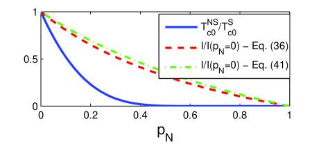
Figure 3: (color online) The transition temperature of the bilayer $T_{c0}^{NS}$, normalized by $T_{c0}^{S}$ (blue solid line) and the first harmonic of the current, divided by its value at $p_{N}=0$, from Eq. (36) (red dashed line). The green dash-dotted line shows the approximation (41) for the current. The parameters used for all graphs are $T_{c0}^{S}=1.27$K (equivalent to $\lambda_{S}=0.17$), $\omega_{D}=400$K, $T_{c0}^{N}=0$ (i.e. $\lambda_{N}=0$) and $1/\tau_{s}=0$. The current is plotted for $T=4T_{c0}^{S}$ and $E_{c}=10T_{c0}^{S}$.

At a fixed $p_{N}$, the persistent current decreases with increasing temperature. Figure 4 shows the current (in units of the Thouless energy $E_{c}$) as a function of the temperature for a specific choice of the parameters and for three values of $p_{N}$. Each of these plots shows the current only above the transition temperature $T^{NS}_{c0}$. As anticipated in the Introduction, the persistent current increases with increasing $E_{c}$. This can be seen from Eqs. (36) and (37), in which the decay of $I$ is determined by the ratio $T/E_{c}$. Using the relation $\widetilde{\cal N}_{\rm eff}T^{S}_{c0}\equiv g/[E_{c}/T^{S}_{c0}]$, where $g$ is the dimensionless conductance, the parameters used in Fig. 4 are equivalent to $g=1000$.

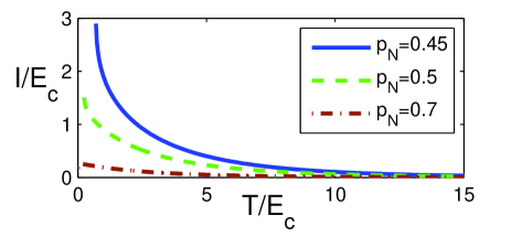
Figure 4: (color online) The first harmonic of the current, in units of the Thouless energy $E_{c}$, versus $T/E_{c}$, for $T_{c0}^{S}=1.27$K, $E_{c}=0.015$K, $\omega_{D}=400$K, $T_{c0}^{N}=1/\tau_{s}=0$ and $\widetilde{{\cal N}}_{\textrm{eff}}T_{c0}^{S}=10^{5}$. The current is plotted for $p_{N}=0.45$, $0.5$, and $0.7$ and for $T>T^{NS}_{c0}(p_{N})$.

Finally, we discuss the effects of a positive transition temperature $T^{N}_{c0}$ and a finite amount of magnetic impurities in the normal slab. Figure 5 shows the first harmonic of the persistent current versus the temperature for $T_{c0}^{N}=1$mK, which is the estimated minimal value for the pure transition temperature of copper derived in Ref. HAMUTAL2, , with and without magnetic impurities. We see that at high temperatures the current is not very sensitive to the pair breaking. As might be expected, the weak superconductivity of the $N$ layer causes an increase in the persistent current.

Interestingly, both Fig. 4 and Fig. 5 exhibit fluctuation-induced persistent currents which are much larger than the Thouless energy $E_{c}$, at temperatures above the superconducting transition temperature of the $S$ material. This persistent current increases, and its decay with temperature becomes slower, as $E_{c}$ increases.

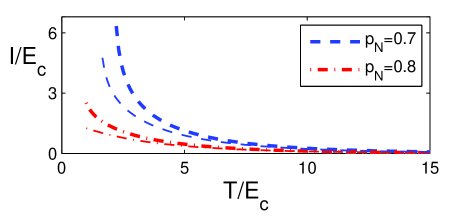
Figure 5: (color online) Same as Fig. 4, but with $T_{c0}^{N}=0.001K$ (i.e. $\lambda_{N}=0.077$). The current is plotted for $p_{N}=0.7$ (blue dashed) and $p_{N}=0.8$ (red dash-dotted). Thick (thin) lines represent $1/\tau_{s}=0$ ($1/\tau_{s}=E_{c}$). The graphs are plotted for $T>T_{c}^{NS}$.

The above plots were based on Eq. (36), which sums over many values of $\ell$ and $j$. For example, Figs. 4 and 5 used $j,\ell\leq 10^{4}$. We next describe approximate expressions, which are valid at high temperatures, when $T\gg T^{NS}_{c0}$. We restrict this discussion to the case $1/\tau_{s}=0$. Defining the small parameter

$$w=-1/\ln[T^{NS}_{c0}/(4\gamma_{E}T)]\ ,$$ (38)

and noting that $\Psi(w-j)\approx-1/w$, we find $F^{j}_{\rm zero}\approx-j+w$, and therefore

$$x^{\ell j}_{\rm zero}\approx x^{\ell j}_{\rm pole}-imw\sqrt{\frac{T}{2\pi E_{c}\bigl{[}1+2j+|\ell|\bigr{]}}}\ .$$ (39)

Inserting this approximation into Eq. (36), the Poisson summation form of the current becomes

$$I \approx-4eT\sum_{m=1}^{\infty}\sin(4\pi m\Phi)\sum_{\ell}\sum_{j=0}^{\infty}\exp[-m\sqrt{2\pi T[1+2j+|\ell|]/E_{c}}\Bigl{[}\exp\bigl{(}mw\sqrt{2\pi T/E_{c}/[1+2j+|\ell|]}\bigr{)}-1\Bigr{]}$$

$$\approx-4eTw\sum_{m=1}^{\infty}\sin(4\pi m\Phi)\sum_{\ell}\sum_{j=0}^{\infty}m\sqrt{2\pi T/E_{c}/[1+2j+|\ell|]}\exp[-m\sqrt{2\pi T(1+2j+|\ell|)/E_{c}}]\ ,$$ (40)

where the last approximation applies only for $mw\sqrt{2\pi T/E_{c}}\ll 1$. At intermediate temperatures, when both this condition and $w\ll 1$ are obeyed, the current decays as $I\approx wI_{1}$, where $I_{1}$ is independent of $T^{NS}_{c0}$. Substituting Eq. (7) for $T^{NS}_{c0}$ in the expression for $w$, we finally end up with

$$\frac{I}{I_{0}}\approx\frac{\ln[4\gamma_{E}T/T^{S}_{c0}]}{\ln[4\gamma_{E}T/T^{S}_{c0}]+\frac{p_{N}(1-\lambda_{N}/\lambda_{S})}{p_{N}\lambda_{N}+p_{S}\lambda_{S}}}\ ,$$ (41)

where $I_{0}$ is the persistent current (for the same flux) at $p_{N}=0$. As seen in Fig. 3, this approximation is quite good.

Unlike the case of the magnetic impurities, in which the persistent current remains non-zero even when the transition temperature vanishes, in the case of the bilayer the persistent current vanishes when $T^{NS}_{c0}=0$. When $\lambda_{N}=0$, the transition temperature approaches zero as $p_{N}$ increases towards the quantum critical point, which occurs at $p_{N}=1$. When $\lambda_{N}<0$, this critical point occurs at a threshold $p^{\times}_{N}<1$, and the fluctuation-induced persistent current vanishes above this threshold. However, as $p_{N}$ approaches this critical threshold, the current decreases linearly with $p_{N}$ [as seen from Eq. (41)]. Since the transition temperature decays exponentially towards that point, we again find that the persistent current remains significant even when the transition temperature is negligibly small!

IV Discussion

The calculations above were carried out within the Gaussian approximation. This approximation usually breaks down close to the phase transition, where higher powers of the order parameters must be taken into account in the expansion of the action ${\cal S}$. This happens below the so-called Ginzburg temperature, $T_{Gi}$. Therefore, one should not trust the above results for temperatures in the range $T^{NS}_{c}<T<T_{Gi}$. In this range, we need to supplement Eq. (17) by the quartic terms, which should be derived by continuing the expansion of Eq. (49) in powers of the $\Delta$’s. In principle, this expansion has the form

$${\cal S}_{4}=\frac{1}{2}\beta\widetilde{\cal N}_{\rm eff}\sum_{\{{\bf q}_{i}\}}\sum_{\nu_{i}}B_{\alpha\beta\gamma\delta}$$

$$\times\Delta_{\alpha}({\bf q}_{1},\nu_{1})\Delta_{\beta}({\bf q}_{2},\nu_{2})\Delta_{\gamma}({\bf q}_{3},\nu_{3})\Delta_{\delta}({\bf q}_{4},\nu_{4})\ ,$$ (42)

where $\alpha,\beta,\gamma,\delta$ take the values $S$ or $N$, and the sums are restricted by $\sum_{i}{\bf q}_{i}=\sum_{i}\nu_{i}=0$.

The calculation of the coefficients $B_{\alpha\beta\gamma\delta}$ goes beyond the scope of the present paper.ALTLAND Usually, these coefficients are assumed to be independent of the momenta ${\bf q}_{i}$ and frequencies $\nu_{i}$, since such dependencies are less relevant near the phase transition in the renormalization group sense. Furthermore, Eq. (18) shows that the interaction terms in Eq. (17), $|\Delta_{S}|^{2}/\lambda_{S}$ and $|\Delta_{N}|^{2}/\lambda_{N}$, are equal to their bulk values multiplied by $p_{S}$ and $p_{N}$, respectively. This indicates a renormalization of $\Delta_{S}$ and $\Delta_{N}$ by the factors $p^{1/2}_{S}$ and by $p^{1/2}_{N}$’ respectively. In analogy, we conjecture that the various coefficients in Eq. (42) are also given by their bulk values, multiplied by the same renormalization factors. We next replace these order parameters by $\Delta_{\pm}$, from Eq. (23). For simplicity, we restrict the following discussion to the special case $\lambda_{N}=0$. This should suffice to demonstrate our arguments. In this special case one has $\lambda_{NS}=p_{S}\lambda_{S}$, $a_{-}=a_{S}=p^{2}_{S}[\lambda^{-1}_{NS}-\gamma]$, $u_{+}=1$ and $u_{-}=0$. Also, $a_{+}=a_{N}=\infty$, and therefore we can ignore all the fluctuations associated with $\Delta_{+}$. Finally, the quartic action becomes

$${\cal S}_{4}=\frac{1}{2}\beta\widetilde{\cal N}_{\rm eff}B_{-}\sum_{\{{\bf q}_{i}\}}\sum_{\nu_{i}}\prod_{i=1}^{4}\Delta_{-}({\bf q}_{i},\nu_{i})\ ,$$ (43)

where again $\sum_{i}{\bf q}_{i}=\sum_{i}\nu_{i}=0$ and we set $B_{-}=p^{2}_{S}B_{0}$, with $B_{0}=7\zeta(3)/(8\pi^{2}T^{2})$ having the bulk value of the quartic term. VARLAMOV Keeping only the first term in Eq. (25), we find the usual structure of the effective Ginzburg-Landau action, except for the renormalization of the coefficients. As we discuss below, the dependence of $a_{-}$ on ${\bf q}$ and on $\nu$ is very different from the simple form used in standard Ginzburg-Landau theories.

The literature contains several ways to estimate the Ginzburg region. Since here we calculate the persistent current, we define that region as the range where the Gaussian calculation presented in the previous section must be modified by inclusion of the quartic terms. Expanding the partition function ${\cal Z}$ to leading order in $B_{-}$, the free energy becomes

$$F=-T\ln{\cal Z}_{\rm fl}+3\widetilde{\cal N}_{\rm eff}B_{-}\Bigl{[}\sum_{\nu}\sum_{\bf q}\langle|\Delta_{-}({\bf q},\nu)|^{2}\rangle\Bigr{]}^{2}\ ,$$ (44)

where $\langle\ldots\rangle$ denotes averaging with the Gaussian action,

$$\langle|\Delta_{-}({\bf q},\nu)|^{2}\rangle=1/[\beta\widetilde{\cal N}_{\rm eff}a_{-}({\bf q},\nu,T)]\ .$$ (45)

The correction to the persistent current due to the quartic term thus becomes

$$\delta I=\frac{3eB_{-}T}{\pi\widetilde{\cal N}_{\rm eff}}\Bigl{[}\sum_{\nu}\sum_{\bf q}\frac{1}{a_{-}}\Bigr{]}\Bigl{[}\sum_{\nu}\sum_{\bf q}\frac{T\partial a_{-}/\partial\Phi}{a^{2}_{-}}\Bigr{]}\ .$$ (46)

The above Gaussian results can be used only if this additional contribution is smaller than that calculated above, Eq. (35).

At $|\Phi|=0$, the denominators in the sums in Eqs. (35) and (46) vanish for $n=\ell=0$, at the critical temperature $T^{NS}_{c0}(\Phi)$ which satisfies Eq. (30). Moving slightly away from this temperature, i.e. at small $T-T^{NS}_{c0}(\Phi)$, each of these sums is dominated by its first term, with $n=\ell=0$. Most of the discussions in the literature proceed by considering only these ‘zero-dimensional classical’ terms.VARLAMOV Following this ‘tradition’, i.e. keeping only these leading terms in all three sums, and comparing $I$ with $\delta I$, we find that for $\Phi\approx 0$ the latter can be neglected if

$$\frac{1}{\lambda_{NS}}-\frac{1}{\lambda_{S}}+\Psi\Bigl{[}\frac{1}{2}+sp_{N}\frac{T^{S}_{c0}}{T}\Bigr{]}-\Psi\Bigl{[}\frac{1}{2}\Bigr{]}+\ln\Bigl{[}\frac{T}{T^{S}_{c0}}\Bigr{]}>\sqrt{\frac{21\zeta(3)}{4\pi^{2}T\widetilde{\cal N}_{\rm eff}p_{S}^{2}}}\ ,$$ (47)

where $s$ was defined after Eq. (8). The left hand side is the denominator for $n=\ell=0$, which vanishes at the mean field transition temperature. Apart from multiplicative factors of order unity, one obtains a similar ‘zero-dimensional classical’ condition using other definitions of the Ginzburg region.VARLAMOV ; FFH Close to the transition at $T^{NS}_{c0}$ one usually replaces $T$ by $T^{NS}_{c0}$ in the denominator of the right hand side. Equation (47) then agrees with the usual Ginzburg criterion in $d$ dimensions, which would give $(T_{Gi}-T_{c})\sim\ln(T_{Gi}/T_{c})\sim T_{c}^{-2/(4-d)}$, with $d=0$, VARLAMOV except for the additional factor $1/p^{2}_{S}$. However, this substitution is problematic when $T^{NS}_{c0}$ is very small, as in our case. Therefore we prefer to keep $T$ also on the right hand side, and then solve Eq. (47) as an equality. For $p_{N}<0.5$ and for the parameters used above, the resulting $T_{Gi}$ turns out to be quite close to $T^{NS}_{c0}$, and therefore the ‘zero-dimensional classical’ Ginzburg region is very narrow. Therefore, Fig. 6 shows these two temperatures only for $p_{N}>0.65$. As seen in this figure, the Ginzburg temperature does not decay as fast as the transition temperature at large values of $p_{N}$. For example, for the value of $\widetilde{{\cal N}}_{\textrm{eff}}T_{c0}^{S}$ used in the figure, we have $T_{Gi}(p_{N}=0.8)=9*10^{-7}T_{c0}^{S}$, while $T_{c0}^{NS}(p_{N}=0.8)=6*10^{-11}T_{c0}^{S}$. In any case, the ‘classical’ Ginzburg region is quite narrow. Had we stopped here (as done in much of the literature), we would conclude that our Gaussian results for the persistent current can be used for practically all temperatures (above $T^{NS}_{c}$) and relative widths of the bilayer.

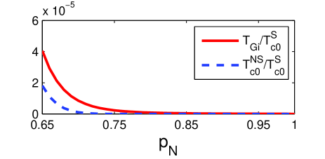
Figure 6: (color online) $T_{Gi}/T_{c0}^{S}$ and $T_{c0}^{NS}/T_{c0}^{S}$ versus $p_{N}$, for $\widetilde{{\cal N}}_{\textrm{eff}}T_{c0}^{S}=10^{5}$. Note the factor of $10^{-5}$ on the $y$-axis.

As one moves away from the critical region, each of the sums in Eqs. (35) and (46) must be supplemented with other terms, involving both non-zero wave vectors ($n\neq 0$) and non-zero Matsubara frequencies ($\ell\neq 0$). In fact, we find that as $n$ increases we need to include more values of $\ell$ to obtain convergence, and that even the Gaussian approximation, on which most of our results are based, requires the summation over many classical and quantum fluctuations. For some reason, most of the literature ignores the ‘quantum’ fluctuations coming from non-zero $\ell$’s, and keeps only the ‘one-dimensional’ terms with $n\neq 0$.VARLAMOV ; fink As discussed above, and in Ref. HAMUTAL2, , the persistent current is affected by both types of fluctuations. The sum in Eq. (35) always converges, becoming of order $1/\ln[T/T^{S}_{c0}]$ for $T^{S}_{c0}\ll T\ll E_{c}$. Similarly, the last sum in Eq. (46) also converges, becoming of order $1/(\ln[T/T^{S}_{c0}])^{2}$. In contrast, the first sum in Eq. (46) does not converge, and thus it depends on the cutoffs imposed on the wave vectors $n$ and on the frequencies $\ell$. This problem arises since our calculation necessitates the replacement of the ‘usual’ Green function $1/(T-T_{c}+\nu+D{\bf q}^{2})$ by $1/[\lambda^{-1}-\gamma({\bf q},\nu,T)]$, with a logarithmic dependence at large $T$, $\nu$ and $q$ [see e.g. Eq. (33)]. Since this sum depends on the cutoffs, the resulting Ginzburg criterion will also depend on these cutoffs.larkin In our case, the dirty diffusive limit imposes the cutoffs $|\nu|,~{}D_{\rm eff}{\bf q}^{2}\ll 1/\tau_{+}$, where $\tau_{+}$ is the elastic mean free time.HAMUTAL2 Replacing the sum $\sum_{\nu,{\bf q}}(1/a_{-})$ by some cutoff dependent constant still shows that $|\delta I/I|$ decreases with increasing $T$. The details of this cutoff dependent criterion go beyond the scope of the present paper.

Our calculation was done for an ensemble of proximity-rings in the same plane. Qualitatively, we expect similar behavior for two rings which are deposited on top of each other, which may be easier to realize experimentally. However, the explicit calculation for the latter case still needs to be carried out. It is also interesting to calculate the persistent current when the bilayer is connected to leads. This also remains for future calculations.

In conclusion, we have demonstrated that the effect of pair weakening due to the proximity between a superconducting ring and a normal (or a weakly superconducting) ring is similar to, but not identical with, that of pair breaking: the persistent current decays slowly with the relative width of the normal layer, and persists even when the superconducting transition temperature (which decays faster) is very small. Since this relative width can be controlled, it would be interesting to check our quantitative predictions experimentally.

Appendix A The partition function

Applying the Hubbard-Stratonovich transformation to Eq. (15), and integrating the fermionic part of the action, the partition function is cast into the form ALTLAND

$${\cal Z} =\int{\cal D}\{\Delta({\bf r},\tau),\Delta^{\ast}({\bf r},\tau)\}e^{-{\cal S}}\ ,$$ (48)

with the action

$${\cal S}=\int d{\bf r}\int_{0}^{\beta}d\tau\frac{|\Delta({\bf r},\tau)|^{2}}{V(x)}-\frac{1}{2}{\rm Tr}\Bigl{\{}\ln\Bigl{(}\beta{\cal G}^{-1}\Bigr{)}\Bigr{\}}\ .$$ (49)

Here $\beta$ is the inverse temperature and ${\cal G}^{-1}$ is the inverse Green function at equal positions and imaginary times,

$${\cal G}^{-1}=\left[\begin{array}[]{cc}G^{-1}_{p}&i\sigma_{y}\Delta\\ (-i\sigma_{y})\Delta^{\ast}&G^{-1}_{h}\end{array}\right]\ ,$$ (52)

with

$$G^{-1}_{p} =\left[\begin{array}[]{cc}-\partial_{\tau}-{\cal H}^{(0)}_{\uparrow\uparrow}&-{\cal H}^{(0)}_{\uparrow\downarrow}\\ -{\cal H}^{(0)}_{\downarrow\uparrow}&-\partial_{\tau}-{\cal H}^{(0)}_{\downarrow\downarrow}\end{array}\right]$$ (55)

being the particle inverse Green function, and

$$G^{-1}_{h} =\left[\begin{array}[]{cc}-\partial_{\tau}+{\cal H}^{(0)}_{\uparrow\uparrow}&{\cal H}^{(0)}_{\downarrow\uparrow}\\ {\cal H}^{(0)}_{\uparrow\downarrow}&-\partial_{\tau}+{\cal H}^{(0)}_{\downarrow\downarrow}\end{array}\right]$$ (58)

being the inverse Green function of the holes. The factor $\beta$ was introduced into the last term in Eq. (49) to keep the argument of the log dimensionless (it does not affect any of the following discussion).

The integration over the bosonic fields in Eq. (48) is carried out using a stationary-phase analysis ALTLAND of the action ${\cal S}$. At temperatures above the transition temperature, this amounts to expanding the second term on the right-hand side of Eq. (49) to second order in $\Delta$ (the first-order contribution to the expansion being zero)

$${\rm Tr}\{\ln(\beta{\cal G}^{-1})\}={\rm Tr}\Bigl{\{}\ln\beta\left[\begin{array}[]{cc}G^{-1}_{p}&0\\ 0&G^{-1}_{h}\end{array}\right]\Bigr{\}}$$ (61)

$$+\int\frac{d{\bf r}d{\bf r}^{\prime}}{\Omega^{2}}\int_{0}^{\beta}\frac{d\tau d\tau^{\prime}}{\beta^{2}}{\cal K}({\bf r},{\bf r}^{\prime},\tau-\tau^{\prime})\Delta({\bf r}^{\prime},\tau^{\prime})\Delta^{\ast}({\bf r},\tau)\ ,$$ (62)

where $\Omega$ denotes the volume of the system (we added the factors of volume and $\beta$ to keep ${\cal S}$ dimensionless). The first term on the right-hand side of Eq. (62) will give the partition function of noninteracting electrons; the second one represents the contribution of the superconducting fluctuations to that function. Its calculation requires the correlation

$${\cal K}({\bf r},{\bf r}^{\prime},\tau-\tau^{\prime}) \equiv-\langle{\rm Tr}\Bigl{\{}G_{p}({\bf r},{\bf r}^{\prime},\tau-\tau^{\prime})\sigma_{y}$$

$$\times G_{h}({\bf r}^{\prime},{\bf r},\tau^{\prime}-\tau)\sigma_{y}\Bigr{\}}\rangle\ ,$$ (63)

where $\langle\ldots\rangle$ indicates averaging over the impurity configurations (see Ref. AGD, for details). Upon averaging, the spatial dependence of ${\cal K}$ becomes a function of $x$, $x^{\prime}$, and ${\mbox{\boldmath{$\rho$}}}-{\mbox{\boldmath{$\rho$}}}^{\prime}$, where ${\mbox{\boldmath{$\rho$}}}\perp\hat{x}$, see Fig. 1. Hence,

$${\rm Tr}\{\ln(\beta{\cal G}^{-1})\}\Big{|}_{\rm 2^{nd}}$$

$$=\int\frac{dxdx^{\prime}}{d^{2}}\sum_{\nu}\sum_{{\bf q}}\Delta_{x^{\prime}}({\bf q},\nu){\cal K}_{xx^{\prime}}({\bf q},\nu)\Delta^{\ast}_{x}({\bf q},\nu)\ ,$$ (64)

where

$${\cal K}_{xx^{\prime}}({\bf q},\nu) =\sum_{{\bf p}_{1},{\bf p}_{2}}\sum_{\omega}\langle{\rm Tr}\Bigl{\{}G(x,x^{\prime},{\bf p}_{1}+{\bf q},{\bf p}_{2}+{\bf q},\omega+\nu)$$

$$\times\sigma_{y}G^{t}(x^{\prime},x,-{\bf p}_{1},-{\bf p}_{2},-\omega)\sigma_{y}\Bigr{\}}\rangle\ ,$$ (65)

and both Green functions are the particle one, HAMUTAL2 i.e., $G=G_{p}$. [In Eq. (64), $d=d_{N}+d_{S}$ is the total width of the sandwich.] We use the notations $\omega\equiv\omega_{n}=\pi T(2n+1)$ for the fermionic Matsubara frequencies, and $\nu\equiv\nu_{\ell}=\pi T2\ell$ for the bosonic frequencies. Note that ${\bf q}$, ${\bf p}_{1}$ and ${\bf p}_{2}$ are two-dimensional vectors normal to $x$.

Inserting these results into the expression for the action [see Eq. (49)], the Gaussian fluctuation-induced partition function, ${\cal Z}_{\rm fl,2}$, takes the form

$${\cal Z}_{\rm fl,2}=\int{\cal D}\{\Delta_{x}({\bf q},\nu),\Delta^{\ast}_{x^{\prime}}({\bf q},\nu)\}e^{-{\cal S}_{2}}\ ,$$ (66)

with

$${\cal S}_{2} =\sum_{\bf q}\sum_{\nu}\int dxdx^{\prime}\Delta^{\ast}_{x}({\bf q},\nu)\Bigl{(}\beta\frac{\delta(x-x^{\prime})}{\widetilde{V}(x)}$$

$$\hskip 28.45274pt-\frac{1}{d^{2}}{\cal K}_{xx^{\prime}}({\bf q},\nu)\Bigr{)}\Delta_{x^{\prime}}({\bf q},\nu)\ ,$$ (67)

(here $\widetilde{V}$ is the attractive interaction. in units of energy $\times$ length). In the Cooper limit, the bosonic variable $\Delta$ takes only two values as a function of $x$, $\Delta_{N}({\bf q},\nu)$ for $0\leq x\leq d_{N}$, and $\Delta_{S}({\bf q},\nu)$ for $-d_{S}\leq x\leq 0$. Therefore the action becomes

$${\cal S}_{2}=\sum_{\bf q}\sum_{\nu}\Delta^{\dagger}({\bf q},\nu)\widetilde{\cal S}({\bf q},\nu)\Delta({\bf q},\nu)\ ,$$ (68)

where

$$\widetilde{\cal S}({\bf q},\nu)=\beta\left[\begin{array}[]{cc}d_{N}\widetilde{\cal N}_{N}\lambda_{N}^{-1}&0\\ 0&d_{S}\widetilde{\cal N}_{S}\lambda^{-1}_{S}\end{array}\right]$$ (71)

$$-\frac{1}{d^{2}}\left[\begin{array}[]{cc}d^{2}_{N}{\cal K}_{NN}({\bf q},\nu)&d_{S}d_{N}{\cal K}_{NS}({\bf q},\nu)\\ d_{N}d_{S}{\cal K}_{SN}({\bf q},\nu)&d^{2}_{S}{\cal K}_{SS}({\bf q},\nu)\end{array}\right]\ ,$$ (74)

$\widetilde{\cal N}_{N(S)}$ denotes the density of states of the normal (superconducting) layer per unit length, and $\Delta^{\dagger}({\bf q},\nu)=\{\Delta^{\ast}_{N}({\bf q},\nu),\Delta^{\ast}_{S}({\bf q},\nu)\}$.

The functions ${\cal K}_{xx^{\prime}}({\bf q},\nu)$, Eq. (65), are calculated by extending the method employed in Refs. DEGENNES, and ANI, to include the dependence on $\nu$ and on the two-dimensional wave vector ${\bf q}$. The calculation is valid in the dirty limit [in which $(D/2\pi T)^{1/2}$ is much larger than the mean-free path of the relevant metal, where $D$ is the diffusion coefficient]. For simplicity, we omit the vector potential from this calculation; its effect is incorporated into the result at the end of Sec. II.

We follow the derivation given in Ref.  DEGENNES, , and begin by presenting the response function ${\cal K}$ in the form

$$\frac{1}{d^{2}}{\cal K}_{xx^{\prime}}({\bf q},\nu) =\sum_{\omega}H_{xx^{\prime}}({\bf q},\nu,\omega)\ .$$ (75)

Had the normal part of the bilayer filled the entire space, then $H_{xx^{\prime}}=H^{(N)}_{xx^{\prime}}$, where

$$H^{(N)}_{xx^{\prime}}({\bf q},\nu,\omega)=\int dq_{x}e^{iq_{x}(x-x^{\prime})}$$

$$\times\frac{\widetilde{\cal N}_{N}}{|2\omega|+|\nu|+2/\tau_{s}+D_{N}({\bf q}^{2}+q^{2}_{x})}\ .$$ (76)

We have allowed for scattering off magnetic impurities in this metal, whose effect is presented by the spin-flip rate $1/\tau_{s}$. (The effect of scattering off nonmagnetic impurities is contained in the diffusion coefficient.) As seen from Eq. (76), the function $H^{(N)}_{xx^{\prime}}$ obeys a diffusion equation

$$\Bigl{(}|2\omega|+|\nu|+2/\tau_{s}+D_{N}{\bf q}^{2}$$

$$-D_{N}\frac{\partial^{2}}{\partial x^{\prime 2}}\Bigr{)}H^{(N)}_{xx^{\prime}}({\bf q},\nu,\omega)=2\pi\widetilde{\cal N}_{N}\delta(x-x^{\prime})\ .$$ (77)

Quite similarly, when the $S$ metal fills the entire space one finds

$$\Bigl{(}|2\omega|+|\nu|+D_{S}{\bf q}^{2}$$

$$-D_{S}\frac{\partial^{2}}{\partial x^{\prime 2}}\Bigr{)}H^{(S)}_{xx^{\prime}}({\bf q},\nu,\omega)=2\pi\widetilde{\cal N}_{S}\delta(x-x^{\prime})\ .$$ (78)

Here it was assumed that the $S$ metal is not doped with magnetic impurities. It follows that in order to find $H_{xx^{\prime}}$ of the double layer, one has to solve the set of equations

$$\Bigl{(}|2\omega|+|\nu|+2/\tau_{s}+D_{N}{\bf q}^{2}-D_{N}\frac{\partial^{2}}{\partial x^{\prime 2}}\Bigr{)}H_{xx^{\prime}}({\bf q},\nu,\omega)=2\pi\widetilde{\cal N}_{N}\delta(x-x^{\prime})\ ,\ \ \ x^{\prime}>0\ ,$$

$$\Bigl{(}|2\omega|+|\nu|+D_{S}{\bf q}^{2}-D_{S}\frac{\partial^{2}}{\partial x^{\prime 2}}\Bigr{)}H_{xx^{\prime}}({\bf q},\nu,\omega)=2\pi\widetilde{\cal N}_{S}\delta(x-x^{\prime})\ ,\ \ x^{\prime}<0\ ,$$ (79)

with the appropriate boundary conditions. Such a scheme has been undertaken in Refs. DEGENNES, and ANI, , leading to the result

$$H_{NN}({\bf q},\nu,\omega)=\frac{\pi\widetilde{\cal N}_{N}^{2}}{d_{N}\widetilde{\cal N}_{N}+d_{S}\widetilde{\cal N}_{S}}\bar{\gamma}({\bf q},\nu,\omega)\ ,$$

$$H_{NS}({\bf q},\nu,\omega)=H_{SN}({\bf q},\nu,\omega)=\frac{\pi\widetilde{\cal N}_{N}\widetilde{\cal N}_{S}}{d_{N}\widetilde{\cal N}_{N}+d_{S}\widetilde{\cal N}_{S}}\bar{\gamma}({\bf q},\nu,\omega)\ ,$$

$$H_{SS}({\bf q},\nu,\omega)=\frac{\pi\widetilde{\cal N}_{S}^{2}}{d_{N}\widetilde{\cal N}_{N}+d_{S}\widetilde{\cal N}_{S}}\bar{\gamma}({\bf q},\nu,\omega)\ ,$$ (80)

where $\bar{\gamma}({\bf q},\nu,\omega)$ was defined in Eq. (20).

Inserting Eqs. (75) and (80) into Eq. (74) brings the action ${\cal S}$, Eq. (68), into the form (17).

References

- (1) M. Büttiker, Y. Imry, and R. Landauer, Phys. Lett. 96A, 365 (1983).
- (2) Y. Imry, Introduction to Mesoscopic Physics, 2nd ed. (Oxford University Press, Oxford, 2002).
- (3) V. Ambegaokar and U. Eckern, Europhys. Lett. 13, 733 (1990).
- (4) V. Ambegaokar and U. Eckern, Phys. Rev. Lett. 65, 381 (1990).
- (5) L. P. Levy, G. Dolan, J. Dunsmuir, and H. Bouchiat, Phys. Rev. Lett. 64, 2074 (1990).
- (6) B. Reulet, M. Ramin, H. Bouchiat, and D. Mailly, Phys. Rev. Lett. 75, 124 (1995).
- (7) R. Deblock, R. Bel, B. Reulet, H. Bouchiat, and D. Mailly, Phys. Rev. Lett. 89, 206803 (2002).
- (8) V. Chandrasekhar, R. A. Webb, M. J. Brady, M. B. Ketchen, W. J. Gallagher, and A. Kleinsasser, Phys. Rev. Lett. 67, 3578 (1991).
- (9) D. Mailley, C. Chapelier, and A. Benoit, Phys. Rev. Lett. 70, 2020 (1993).
- (10) W. Rabaud, L. Saminadayar, D. Mailly, K. Hasselbach, A. Benoit, and B. Etienne, Phys. Rev. Lett. 86, 3124 (2001).
- (11) H. Bluhm, N. C. Koshnick, J. A. Bert, M. E. Huber, and K. A. Moler, Phys. Rev. Lett. 102, 136802 (2009).
- (12) E. M. Q. Jariwala, P. Mohanty, M. B. Ketchen, and R. A. Webb, Phys. Rev. Lett. 86, 1594 (2001).
- (13) A. C. Bleszynski-Jayich, W. E. Shanks, B. Peaudecerf, E. Ginossar, F. von Oppen, L. Glazman, and J. G. E. Harris, Science 326, 272 (2009).
- (14) E. Ginossar, L. I. Glazman, T. Ojanen, F. von Oppen, W. E. Shanks, A. C. Bleszynski-Jayich, and J. G. E. Harris, Phys. Rev. B 81, 155448 (2010).
- (15) See also e.g. H. Bary-Soroker, O. Entin-Wohlman, and Y. Imry, Phys. Rev. B 82, 144202 (2010).
- (16) C. Vallette, Solid State Comm. 9, 895 (1971).
- (17) G. Deutscher, S. Y. Hsieh, P. Lindenfeld, and S. Wolf, Phys. Rev. B 8, 5055 (1973).
- (18) G. Deutscher, Solid State Comm. 9, 891 (1971).
- (19) H. Bouchiat, Physics 1, 7 (2008).
- (20) H. Bary-Soroker, O. Entin-Wohlman, and Y. Imry, Phys. Rev. Lett. 101, 057001 (2008).
- (21) H. Bary-Soroker, O. Entin-Wohlman, and Y. Imry, Phys. Rev. B 80, 024509 (2009).
- (22) F. Pierre, A. B. Gougam, A. Anthore, H. Pothier, D. Esteve, and N. O. Birge, Phys. Rev. B 68, 085413 (2003).
- (23) G. Schwiete and Y. Oreg, Phys. Rev. Lett. 103, 037001 (2009); Phys. Rev. B 82, 214514 (2010).
- (24) P. G. de Gennes, Rev. Mod. Phys. 36, 225 (1964).
- (25) O. Entin-Wohlman, Phys. Rev. B 12, 4860 (1975).
- (26) P. Fulde, in Bardeen Cooper and Schrieffer: 50 years, eds. L. N. Cooper and D. Feldman (World Scientific, 2010).
- (27) The coherence length, in the dirty limit, is given by ; the dirty-limit condition is , where is the elastic mean-free path.
- (28) W. L. McMillan, Phys. Rev. 175, 537 (1968).
- (29) A. A. Abrikosov and L. P. Gorkov, Soviet Physics JETP 12, 1243 (1961).
- (30) A. A. Abrikosov, L. P. Gorkov, and I. E. Dzyaloshinskii, Methods of Quantum Field Theory in Statistical Physics (Prentice-Hall, Englewood Cliffs, NJ, 1963).
- (31) A. Altland and B. Simons, Condensed Matter Field Theory (Cambridge University Press, Cambridge, 2006).
- (32) C. Caroli and K. Maki, Phys. Rev. 159, 306 (1967).
- (33) A. I. Larkin and A. Varlamov, Theory of Fluctuations in Superconductors (Oxford University Press, 2009).
- (34) D. S. Fisher, M. P. A. Fisher and D. Huse, Phys. Rev. B 43, 130 (1991).
- (35) An exception was treated by K. Michaeli and A. M. Finkel’stein, Phys. Rev. B 80, 214516 (2009).
- (36) See e.g. V. M. Galitsky and A. I. Larkin, Phys. Rev. B 63, 174506 (2001); V. M. Galitski, Phys. Rev. Lett. 100, 127001 (2008).