Diffuse neutral hydrogen in the H i Parkes All Sky Survey

Abstract

Context. Observations of neutral hydrogen can provide a wealth of information about the distribution and kinematics of galaxies. To learn more about large scale structures and accretion processes, the extended environment of galaxies must also be observed. Numerical simulations predict a cosmic web of extended structures and gaseous filaments.

Aims. To detect H i beyond the ionisation edge of galaxy disks, column density sensitivities have to be achieved that probe the regime of Lyman limit systems. Typically H i observations are limited to a brightness sensitivity of $N_{HI}\sim 10^{19}$ cm^-2 but this has to be improved by at least an order of magnitude.

Methods. In this paper, reprocessed data is presented that was originally observed for the H i Parkes All Sky Survey (HIPASS). HIPASS provides complete coverage of the region that has been observed for the Westerbork Virgo Filament H i Survey (WVFS), presented in accompanying papers, and thus is an excellent product for data comparison. The region of interest extends from 8 to 17 hours in right ascension and from $-$1 to 10 degrees in declination. Although the original HIPASS product already has good flux sensitivity, the sensitivity and noise characteristics can be significantly improved with a different processing method.

Results. The newly processed data has an $1\sigma$ RMS flux sensitivity of $\sim 10$ mJy beam^-1 over 26 km s^-1, corresponding to a column density sensitivity of $\sim 3\cdot 10^{17}$ cm^-2. While the RMS sensitivity is improved by only a modest 20%, the more substantial benefit is in the reduction of spectral artefacts near bright sources by more than an order of magnitude. In the reprocessed region we confirm all previously catalogued HIPASS sources and have identified 29 additional sources of which 14 are completely new H i detections. We derived spectra and moment maps for all detections together with total fluxes determined both by integrating the spectrum and by integrating the flux in the moment maps within the source radius. Extended emission or companions were sought in the nearby environment of each discrete detection. Ten extra-galactic filaments are marginally detected within the moment maps.

Conclusions. With the improved sensitivity after reprocessing and its large sky coverage, the HIPASS data is a valuable resource for detection of faint H i emission. This faint emission can correspond to extended halos, dwarf galaxies, tidal remnant and potentially diffuse filaments that represent the trace neutral fraction of the Cosmic Web.

1 Introduction

Current cosmological models ascribe about 4% of the density to baryons (Spergel et al., 2007). At low redshift most of these baryons do not reside in galaxies, but are expected to be hidden in extended gaseous web-like filaments. (e.g. Davé et al. (1999), Davé et al. (2001), Cen & Ostriker (1999)). Calculations suggets that in the current epoch baryons are almost equally distributed amongst three components: (1) galactic concentrations, (2) a warm-hot intergalactic medium (WHIM) and (3) a diffuse intergalactic medium (seen as the Ly$\alpha$ forest). These simulations predict that the three components are each coupled to a decreasing range of baryonic overdensity $\log(\rho/\bar{\rho}_{H})>3.5$, 1 - 3.5, and $<3.5$.

Direct detection of the inter-galactic gas, or the WHIM, is very difficult in the EUV and X-ray bands (Cen & Ostriker, 1999). In this and accompanying papers we make an effort to detect traces of the inter and circum-galactic medium in neutral hydrogen. Due to the moderately high temperatures in the intergalactic medium (above $10^{4}$ Kelvin), most of the gas in the Cosmic Web is highly ionised. To detect the trace neutral fraction in the Lyman Limit Systems using the 21-cm line of neutral hydrogen, a column density sensitivity of $N_{HI}\sim 10^{17-18}$ is required. A more detailed background and introduction to this topic is given in Popping (2010) and Popping & Braun (2011a).

A first example of detection in H i emission of the likely counterpart of a Lyman Limit absorption System is shown in Braun & Thilker (2004), where a very diffuse H i structure is seen with a peak column density of only $N_{HI}\sim 10^{18}$ cm^-2, connecting M31 and M33. To be able to detect a large number of diffuse H i features, extended blind surveys are required with an excellent brightness sensitivity. One of the first such efforts is presented in Popping & Braun (2011a), where the Westerbork Synthesis Radio Telescope (WSRT) is used to undertake a deep fully-sampled survey of the galaxy filament joining the Local Group to the Virgo Cluster (Westerbork Virgo Filament H i Survey) extending from 8 to 17 hours in RA and from $-$1 to +10 degrees in Declination. Data products were created from both the cross-, as well as the auto-correlation data, to achieve a very high brightness sensitivity at a variety of spatial resolutions. The total-power product of the WVFS is presented in Popping & Braun (2011a), while the interferometric data is presented in Popping & Braun (2011b). In these papers new detections of neutral hydrogen are reported. Although these detections are very interesting, they are difficult to interpret or to confirm, as no comparison data is currently available at a comparable sensitivity.

In this paper we use reprocessed data of the H i Parkes All Sky Survey to complement the WVFS observation. The H i Parkes All Sky Survey (HIPASS) (Barnes et al., 2001) includes the complete Southern sky and the Northern sky up to +25.5 degrees in Declination. The Northern part of the survey is described in Wong et al. (2006). This survey currently has the best available H i brightness sensitivity yet published. As the Northern part of the survey completely covers the region that has been observed for the Westerbork Virgo Filament Survey, HIPASS is an excellent product for data comparison.

Although neither the flux sensitivity, nor the brightness sensitivity of HIPASS is equivalent to that of the WVFS total power data, we can still learn more about faint H i detections in the WVFS, by taking into account the limitations of both surveys. The low column densities of some new H i detections in the WVFS might be confirmed, indicating that the gas is indeed very diffuse. Conversely, if column densities measured in the HIPASS data are significantly higher than in the WVFS, this would imply that the gas is more condensed than it appeared, with the emission diluted by the large beam of the WVFS.

Although the HIPASS data is completely reduced and the processed cubes are publicly available, for our purpose we have begun anew with the raw, unprocessed observational data. Increased computing capacity, and different calibration algorithms allow significant improvements to be achieved over the original HIPASS products.

In the observations and data reduction sections we will explain in detail the processing employed and the improvements achieved. A new list of objects detected in the region of interest is given in the results section. Although the improved data reduction method can be applied to the complete HIPASS survey area, we emphasise that we have only applied it to the region of overlap with the WVFS both spatially and spectrally.

In section 2 of this paper we will briefly summarise the observations that have been used, followed by the data reduction strategy in section 3. In section 4 the results will be presented; the general properties of each detected object are given, but new H i detections in the HIPASS data are discussed in more detail. We close with a short discussion and conclusion in sections 5 and 6. Detailed analysis and comparison of the data, together with a discussion of the nature of the H i emission will be presented in a future paper. In that paper we will compare the results of the HIPASS data together with the auto- and cross-correlation products of the WVFS.

2 Observations

In our search for diffuse H i emission, we have employed data that was originally acquired for the H i Parkes All Sky Survey (HIPASS). The data is described in detail in Barnes et al. (2001) and we will only summarise the relevant properties. All data has been obtained using the Parkes 21-cm Multibeam system, containing a cooled 13 beam receiver and digital correlator. The Multibeam correlator has an instantaneous bandwidth of 64 MHz divided into 1024 channels. For the HIPASS observations the receivers were tuned to a central frequency of 1394.5 MHz, offering a velocity range of $-$1280 to 12700 km s^-1 with a mean channel separation of 13.4 km s^-1. The central beam FWHM is 14.0 arcmin, and the 13 beams are separated from one another by about 30 arcmin. Data acquisition was started in 1997 February and completed in 2000 March. Observations were obtained by scanning the Telescope in Declination strips of 8 degrees length. The multibeam receiver is rotated relative to the scan direction, to get approximately uniformly spaced sampling of the sky over a strip of $\sim 1.7$ degrees width. Each Declination scan maps approximately $8\times 1.7$ degrees. To obtain full coverage of the sky at full sensitivity, subsequent scans are displaced by 7 arcmin in RA, which means that each of the 13 beams maps the sky with Nyquist sampling. The scan rate of each strip is 1 degree min^-1. Using all 13 beams, the total integration time of the HIPASS survey results in $7\times 10^{3}$ s deg^-2, or 450 s beam^-1. The typical sensitivity of the original HIPASS product is 13.3 mJy beam^-1 over 18 km s^-1.

For the original HIPASS product, cubes were created of $8\times 8$ degrees in size, centered at Declinations between $-$90 and +24 degrees. For our purpose we have selected all original HIPASS scans centered at a Declination of $-$2, 6 and 14 degrees, and between 8 and 17 hours in Right Ascension. With these data we achieve the best possible coverage and sensitivity in the region between $-$1 and 10 degrees in Declination. This region was selected to exactly overlap with the region observed in the Westerbork Virgo Filament Survey (WVFS). The WVFS is an unbiased survey of $\sim 1500$ squared degrees, undertaken with the Westerbork Synthesis Radio Telescope (WSRT), directed at the galaxy filament connecting the Local Group with the Virgo Cluster. The WVFS total power data has an effective beam size of $\sim 49$ arcmin with a sensitivity of 16 mJy beam^-1 over 16 km s^-1. The HIPASS data has a slightly superior flux sensitivity, but because of the smaller beam size the column density sensitivity is about an order of magnitude worse. Nevertheless the HIPASS data is an excellent product to use for comparison with the WVFS data.

3 Data Reduction

3.1 Bandpass removal in the original HIPASS product

Although the original unprocessed HIPASS data have been used, the reduction method is slightly different, to obtain an improved end product. The most challenging aspect of calibrating an observed total power spectrum is the accurate estimation of the system bandpass shape. Bandpass calibration of a single dish telescope is traditionally accomplished by observing in signal/reference mode. The telescope alternately tracks the target position and a suitable nearby reference region for the same amount of time. The reference position is used to estimate the bandpass shape and is divided out of the signal spectrum. For HIPASS the telescope was scanning the sky continuously, so the straight-forward signal/reference method could not be employed. The method that has been used, was to estimate the bandpass shape of each spectrum, by using a combination of earlier and later spectra, observed by the same feed of the multibeam receiver. The bandpass was estimated by taking a channel-by-channel median of the earlier and later spectra. The median reference spectrum was preferred above the mean reference spectrum, as the median statistic is more robust to outlying data points, and is independent of the magnitude of deviation of outlying points.

The strategy that has been used in reducing the raw HIPASS data works well in the absence of line emission, but breaks down in the vicinity of bright detections. Some H i sources are sufficiently bright that bandpass estimates just prior and after the target spectrum are elevated by the source itself. This results in negative artefacts, or bandpass sidelobes that appear as depressions in the spectra north and south of strong H i sources.

3.2 Bandpass removal in reprocessed HIPASS data

All unprocessed HIPASS spectra are archived and can be reprocessed using different methods. Techniques can be developed to improve the bandpass-sidelobes and preserve spatially extended emission. An example of such an approach is given by Putman et al. (2003) where a different processing algorithm has been employed to image HVCs and the Magellanic Stream. We have tested many different algorithms, including the original HIPASS processing pipeline and the method used by Putman et al. (2003), and achieved the lowest residual RMS fluctuation level with the approach outlined below.

The data were bandpass-corrected, calibrated and Doppler-tracked using the aips++ program LiveData (Barnes et al., 2001) in the following manner.

• The spectra were hanning smoothed over three channels to a velocity resolution of $\sim 26$ km s^-1.

• In estimating the shape of the bandpass, a complete 8^∘ scan is used instead of just a few time steps before and after the target spectrum. By using a complete scan instead of a subset the statistics are improved, making the bandpass estimate more robust.

• A third order polynomial has been fit to the data in the time domain. Data points outside 2 times the standard deviation were excluded from the polynomial fit. This process is iterated three times, to get the best possible outlier rejection.

• After fitting and correcting the data in the time domain, a second order polynomial was fit in the frequency domain. Higher order polynomials in frequency were tested but did not improve the result.

All the processed scans were gridded with Gridzilla (Barnes et al., 2001) using a pixel size of 4’. Cubes were created with a size of 24 degrees in Declination, ranging from $-$6 to 18 degrees and typical width of 1 hour in Right Ascension with an overlap of one degree between the adjacent cubes.

All overlapping scans were averaged using the system temperature weighted median of relevant data points. The value of the median is strongly dependent on the form of the weighting function w(r) and the radius $r_{max}$ out to which spectra are included. The weighting procedure for HIPASS is described in detail in Barnes et al. (2001). A Gaussian beam-shape is assumed, so the weighting function has the functional form:

$$w(r)=\left\{\begin{array}[]{l l}\exp\Big{[}-\big{(}\frac{r}{\sigma}\big{)}^{2}/2\Big{]}&\quad\mbox{for $r\leq r_{max}$}\\ 0&\quad\mbox{for $r>r_{max}$}\\ \end{array}\right.$$ (1)

For gridding the HIPASS data, a value of $r_{max}=6$ arcmin. has been adopted. The estimated flux at a given pixel is determined by the weighted median of all spectra contributing to that pixel and has the form:

$$F_{e}=\frac{\textrm{median}(F)}{\textrm{median}(w)}$$ (2)

For a random distribution of data points or observations, the median of the weights [median($w$)] is determined by the weighting function where the radius divides the smoothing area in two equivalent parts, i.e. $w(r_{max}/\sqrt{2})$. For the adopted $r_{max}$ of 6 arcmin, median($w$)=1.28, which has been taken into account when gridding the data. Tests during the gridding of HIPASS data have shown that the input spectra are very nearly randomly distributed on the sky (Barnes et al., 2001).

A top-hat kernel of 12’ has been used to smooth data spatially. The final beam size of the gridded data cubes is approximately 15.5’ FWHM, although as discussed at some length in Barnes et al. (2001), the effective beam-size is dependent on the signal-to-noise ratio of a detection.

After the processed cubes were formed, sub-cubes were created using the inner 14 degrees in Declination with the highest uniform sensitivity overlapping with the WVFS data. A velocity range was selected from 200 to 1700 km s^-1, again to match with the velocity coverage of the WVFS data.

In the reprocessed data, we typically achieve an RMS flux sensitivity of $\sim 10$ mJy beam^-1 over 26 km s^-1. This is an improvement on the original HIPASS processing, although we have degraded the velocity resolution to 26 km s^-1 compared to 18 km s^-1, due to the Hanning smoothing that has been used instead of the Tukey smoothing. When scaling both noise values to the same velocity resolution, the achieved sensitivity is a significant improvement on the sensitivity of the first HIPASS product. The typical sensitivity of the first HIPASS product is $\sim 13$ mJy beam^-1 over 18 km s^-1. For the northern Declinations we are concentrating on, the sensitivity is slightly worse at $\sim 14$ mJy beam^-1 over 18 km s^-1 (Wong et al., 2006) corresponding to $\sim 12$ mJy beam^-1 over 26 km s^-1. The previous reprocessing of the HIPASS data (Putman et al., 2003) resulted in a similar rms value as we are achieving, however was not able to correct for the negative artefacts. Rather than an improved rms value, the more important benefit of reprocessing the data is that the negative artefacts in the vicinity of bright sources are suppressed by more than an order of magnitude.

An example of the reduced data and its artefacts is given in Fig. 1. The left panel shows a region of the sky processed with the original HIPASS pipeline. There are strong negative artefacts north and south of strong H i sources. The right panel of Fig. 1 shows the same region processed with the improved reduction pipeline. Although the spectral artefacts are still visible, there is a dramatic improvement. The reprocessed data will be much more sensitive to diffuse H i emission, especially in the direct vicinity of bright H i objects. Using this follow-up HIPASS product, better flux estimates can be determined for discrete sources. Moreover, it also allows investigation of the nearby environment of discrete bright objects, which has previously been impossible.

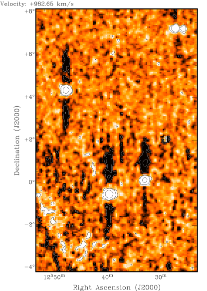
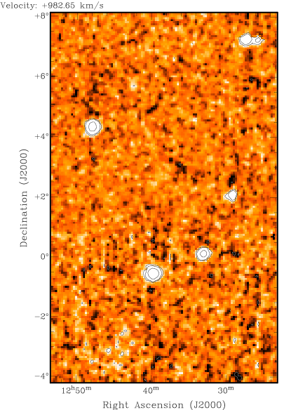
Figure 1: Example of the artefacts in the original HIPASS pipeline (left panel) and the reprocessed data (right panel). Both panels show the same region of the sky at the same velocity, the intensity ranges from -40 to 40 mJy beam^-1. Contours are plotted at -60, -30, 30, 60 and 300 mJy beam^-1, negative contours are coloured white

4 Results

A significant sky area of more than 1500 deg² has been reprocessed from the original HIPASS data. We achieve an RMS sensitivity that is improved by $\sim 20$% compared to the published HIPASS product. More important than this improvement in noise, is the very effective suppression of the negative artefacts surrounding all bright H i detections. We expect slightly different flux values, especially for the bright H i objects, as the newly processed data is more sensitive to extended emission. Furthermore, we expect to have more H i detections of diffuse or companion galaxies due to the improved sensitivity and artefact suppression.

For the detection of sources we have used two methods. Firstly an automated source finder was employed to identify sources. Developing a fully automated and reliably source finder is extremely difficult, especially when looking for faint objects, therefore all the cubes were also inspected visually to identify features that might be missed by the automated source finder.

4.1 Automatic source detection

We use the Duchamp (Whiting, 2008) three dimensional source finding algorithm to identify candidate detections. Features are sought with a peak flux exceeding 5 times the noise value. Detections are grown down from the peak to a cutoff value of three times the noise, to be more sensitive to extended or diffuse emission. The requirement for candidate sources to be accepted is to have a size of at least 10 pixels (after growing) in one channel and to contain pixels from at least 2 adjacent channels. As a result the minimum velocity width of a detection is 26 km s^-1 which is sufficient to detect most galaxies, but low mass dwarf galaxies or companions might be missed. The search criteria were chosen to eliminate isolated noise peaks and make the detections more reliable.

The original reduced data has a velocity resolution of 26 km s^-1. Hanning smoothed versions of the data cubes have been created at a velocity resolution of 52 and 104 km s^-1. These smoothed cubes are more sensitive to structures that are extended in the velocity domain. Duchamp was applied in a similar way as to the original data cubes, however this did not result in additional detections.

Spectra and moment maps of all the candidate detections have been inspected visually for reliability. Strong artefacts due to e.g. solar interference can be easily identified in the integrated maps and these features were eliminated from the source list. The spectra can be used to identify false detections that are caused by ripples in the bandpass seen toward continuum sources.

4.2 Visual source detection

Although automatic source finders are an excellent tool to search for candidate detections they have their limitations. Detecting point sources is relatively easy, as they are clearly defined in both the spatial and velocity domain. We are especially interested in diffuse features that have a peak brightness of only a few times the noise. These sources can only be found when source finders are ”tuned” to the actual properties, the spatial and spectral extent, of these features. Since we do not know the appearance or existence of the sources beforehand, it is difficult to employ dedicated source finders. Another complication is that the noise is not completely uniform. The noise can be elevated, for example, in the vicinity of continuum sources or in the case of solar interference. Several efforts have been made to look for diffuse but very extended features, both spatially and in velocity. Unfortunately these efforts have not been very successful and resulted in previously known or unreliable detections.

Visual inspection of the data was necessary, to have a better understanding of the quality and features in the data, but also to look for features that have been missed by the automated source finder. All cubes were inspected in the spatial domain as well as in the two velocity domains (RA versus velocity and Dec versus velocity) to search for objects that had been missed.

4.3 Detected sources

For each candidate detection an optical counterpart was sought in the NASA Extragalactic Database (NED) within a search radius of 14 arcmin. This radius is approximately the diameter of the HIPASS beam and only objects within this radius can contribute to the measured flux. Another requirement for potential optical counterparts is to have a known radial velocity that is comparable to the radial velocity of the H i detection. Candidate detections with a clearly identified optical counterpart are accepted. For each candidate detection the noise is determined based on the line-width at 20% of the peak ($W_{20}$). For line-widths smaller than 250 km s^-1 the noise is given as:

$$n=\sqrt{\frac{1.5W_{20}}{v_{res}}}\cdot\textrm{RMS}\cdot v_{res}$$ (3)

where $n$ is in units of [Jy km s^-1], RMS is the sensitivity of the cubes and $v_{res}$ is the velocity resolution. For broader profiles the term $(1.5W_{20})$ is replaced by ($W_{20}+50$ km s^-1) to account for the line wings.

Using this noise measurement, a signal-to-noise ratio can be determined for each candidate detection. Candidate detections with an integrated signal-to-noise larger than 5 are accepted as detections.

Finally, a list of 203 detections was obtained of which 31 were detected by visual inspection; all detections and their observed properties are listed in table. LABEL:sources. The first column gives the catalogue name, composed of the three characters ”HIR”, an abbreviation of ”HIPASS Reprocessed”, followed by two sets of four digits indicating the Right Ascension and Declination of the detection. The second column gives the optical identification of the detection if any is known and the third column gives the original HIPASS ID if available. Completely new H i detections are indicated in the third column by ”new”. In the case a detections is not mentioned in the HIPASS catalogue however is detected by ALFALFA, this is indicated with ”$\alpha\alpha$”. The fourth, fifth and sixth column give the spatial position and heliocentric velocity of the source. This is followed by velocity width of the object, at 20% of the peak flux. The seventh and eighth columns give the integrated flux (3-D) and the integrated line-strength (1-D) respectively. We will discuss the differences between the two different flux measurements in the following section. The last column indicates whether the object is detected by the automatic source finder (A) or by visual inspection (V). In some cases the objects are completely at the edge of the processed bandwidth. Although a detection here can be a solid detection, the estimated flux and line-width values are underestimated as a part of the spectrum is missing. For objects at the edge of the bandwidth, this is indicated in the table with a letter ${}^{\prime\prime}(u)^{\prime\prime}$

Table 1: Observed properties of H i detections in reprocessed HIPASS data within the Westerbork Virgo Filament Survey region (a): Units of $V_{Hel}$ are given in [km s^-1]. (b): Units of $W_{20}$ are given in [km s^-1]. (c): Units of $S_{int}$ are given in [Jy km s^-1]. (d): Units of $S_{line}$ are given in [Jy km s^-1]. (u): The flux and line-width values are underestimated as the object is at the edge of the processed bandwidth..

Name	Optical ID.	HIPASS ID	RA [hh:mm:ss]	Dec [dd:mm:ss]	$V_{Hel}$(a)	$W_{20}$(b)	$S_{int}$(c)	$S_{line}$(d)	det.
HIR0821-0025	UGC 04358	HIPASS J0821-00	8:21:41	-0:25:00	1775u	50u	4.1u	3.5u	A
HIR0859+1109	UGC 04712	new	8:59:28	11:09:23	1643	80	1.9	3.0	A
HIR0906+0618	UGC 04781	HIPASS J0906+06	9:06:36	6:18:27	1433	168	19.7	16.0	A
HIR0908+0555	UGC 04797	HIPASS J0908+05a	9:08:12	5:55:54	1326	102	5.6	5.3	A
HIR0908+0517	SDSS J090836.54+051726.8	HIPASS J0908+05b	9:08:43	5:17:49	600	57	1.3	2.2	A
HIR0910+0711	NGC 2777	HIPASSJ0910+07	9:10:34	7:11:43	1500	139	11.6	9.9	A
HIR0911+0024	No object found.	new	9:11:21	0:24:59	1286	83	2.8	2.7	A
HIR0921+0725	No object found.	new	9:21:07	7:25:32	1369	110	3.7	4.5	A
HIR0944-0038	UGC 05205	HIPASS J0944-00a	9:44:06	-0:38:42	1485	178	15.0	13.1	A
HIR0944+0937	IC 0559	HIPASS J0944+09	9:44:31	9:37:06	522	132	5.6	4.8	A
HIR0944-0040	SDSS J094446.23-004118.2	HIPASS J0944-00b	9:44:43	-0:40:37	1222	161	7.0	8.5	A
HIR0946+0141	SDSS J094602.54+014019.4	new	9:46:00	1:41:07	1763u	53u	1.0u	2.3u	A
HIR0946+0031	UGC 05238	HIPASS J0946+00	9:46:55	0:31:09	1697u	120u	7.0u	7.7u	A
HIR0947+0241	UGC 05249	HIPASS J0947+02	9:47:44	2:41:15	1776	25	1.3	1.6	A
HIR0951+0750	UGC 05288	HIPASS J0951+07	9:51:16	7:50:12	555	112	33.0	27.8	A
HIR0953+0135	NGC 3044	HIPASS J0953+01	9:53:42	1:35:06	1292	341	47.3	49.4	A
HIR0954+0915	NGC 3049	HIPASS J0954+09	9:54:41	9:15:53	1471	223	6.1	9.1	A
HIR1005+0139	2dFGRS N421Z115	new	10:05:20	1:39:48	1260	95	2.0	2.4	V
HIR1007+1022	UGC 05456	HIPASS J1007+10	10:07:18	10:22:18	547	90	4.8	7.2	A
HIR1013+0702	UGC 05522	HIPASS J1013+07	10:13:57	7:02:36	1219	232	44.7	42.8	A
HIR1014+0329	NGC 3169	HIPASS J1014+03	10:14:17	3:29:28	1246	457	141.4	98.7	A
HIR1015+0242	UGC 05539	HIPASS J1015+02	10:15:52	2:42:11	1275	157	11.4	13.7	A
HIR1017+0421	UGC 05551	HIPASS J1017+04	10:17:12	4:21:37	1340	90	9.4	6.0	A
HIR1028+0335	UGC 05677	HIPASS J1028+03	10:28:33	3:35:28	1146	139	3.2	5.4	A
HIR1031+0428	UGC 05708	HIPASS J1031+04	10:31:15	4:28:27	1169	198	33.9	33.9	A
HIR1038+1024	CGCG 065-074	HIPASS J1038+10	10:38:14	10:24:26	1167	192	8.1	6.9	A
HIR1039+0145	UGC 05797	HIPASS J1039+01	10:39:28	1:45:15	706	71	3.9	3.0	A
HIR1044+1134	MESSIER 095	HIPASS J1044+11	10:44:02	11:34:18	798	280	12.2	32.8	A
HIR1046+0149	NGC 3365	HIPASS J1046+01	10:46:11	1:49:32	985	248	36.1	43.1	A
HIR1051+0550	NGC 3423	HIPASS J1051+05	10:51:17	5:50:24	1010	186	42.4	45.8	A
HIR1051+0327	HIPASS J1051+03	HIPASS J1051+03	10:51:31	3:27:20	1062	85	13.0	13.3	A
HIR1051+0435	UGC 05974	HIPASS J1051+04	10:51:34	4:35:53	1050	175	11.1	15.3	A
HIR1052+0002	MGC 0013223	new	10:52:49	0:02:35	1776u	30u	1.3u	1.2u	A
HIR1053+0232	LSBC L1-137	HIPASS J1053+02	10:53:08	2:32:41	1035	89	6.4	6.4	A
HIR1055+0511	No object found.	new	10:55:27	5:11:57	982	142	6.4	3.8	V
HIR1101+0338	NGC 3495	HIPASS J1101+03	11:01:15	3:38:01	1119	324	27.4	30.5	A
HIR1105-0002	NGC 3521	HIPASS J1105-00	11:05:48	-0:02:05	793	444	298.8	199.0	A
HIR1107+0710	NGC 3526	HIPASS J1106+07	11:07:00	7:10:54	1422	194	10.6	6.6	A
HIR1110+0107	CGCG 011-018	HIPASS J1110+01	11:10:56	1:07:45	983	96	3.4	5.1	A
HIR1112+1014	UGC 06248	HIPASS J1112+10	11:12:45	10:14:03	1286	75	1.8	2.7	A
HIR1117+0434	NGC 3604	HIPASS J1117+04	11:17:30	4:34:25	1511	209	7.9	10.8	A
HIR1119+0939	SDSS J111928.10+093544.2	HIPASS J1119+09	11:19:46	9:39:12	1075	298	4.6	3.6	V
HIR1120+0232	UGC 06345	HIPASS J1120+02	11:20:11	2:32:48	1604	141	19.7	22.0	A
HIR1124+0318	NGC 3664	HIPASS J1124+03	11:24:25	3:18:44	1379	140	20.5	22.7	A
HIR1124+1121	NGC 3666	HIPASS J1124+11	11:24:25	11:21:16	1056	278	41.0	45.9	A
HIR1125+0958	IC 0692	HIPASS J1126+10	11:25:53	9:58:09	1154	102	3.1	3.5	A
HIR1127+0846	IC 2828	HIPASS J1127+08	11:27:03	8:46:06	1048	79	1.0	1.6	V
HIR1127-0058	UGC 06457	HIPASS J1127-00	11:27:10	-0:58:30	956	106	7.2	7.9	A
HIR1128+0923	NGC 3692	HIPASS J1128+09a	11:28:19	9:23:35	1617	236	11.7	9.4	A
HIR1130+0917	NGC 3705	HIPASS J1130+09	11:30:02	9:17:38	1018	353	29.6	34.4	A
HIR1136+0049	UGC 06578	HIPASS J1136+00b	11:36:32	0:49:04	1099	95	5.5	5.7	A
HIR1140+1128	NGC 3810	HIPASS J1140+11	11:40:59	11:28:07	995	268	33.6	38.5	A
HIR1144+0210	SDSS J114454.28+020946.8	HIPASS J1145+02	11:44:52	2:10:15	1009	52	4.1	3.5	A
HIR1158-0127	UGC 06970	HIPASS J1158-01	11:58:41	-1:27:28	1471	166	46.4	4.4	A
HIR1200-0105	NGC 4030	HIPASS J1200-01	12:00:26	-1:05:52	1465	346	64.0	50.8	A
HIR1204-0131	UGC 07053	HIPASS J1204-01	12:04:17	-1:31:37	1469	123	6.5	8.2	A
HIR1207+0249	HIPASS J1208+02	HIPASS J1208+02	12:07:57	2:49:05	1318	220	84.7	55.7	A
HIR1211+0201	UGC 07178	HIPASS J1211+02a	12:11:04	2:01:37	1334	95	6.2	8.0	A
HIR1211+0256	UGC 07185	HIPASS J1211+02b	12:11:26	2:56:53	1300	110	5.8	7.6	A
HIR1212+0248	LEDA 135791	new	12:12:27	2:48:29	877	117	3.1	3.9	A
HIR1212+1054	NGC 4178	HIPASS J1212+10	12:12:51	10:54:29	476u	56u	10.0u	8.7u	A
HIR1214+0747	UGC 07239	HIPASS J1214+07	12:14:12	7:47:05	1220	148	5.3	5.3	A
HIR1214+0911	VCC 0117	HIPASS J1214+09	12:14:48	9:11:33	1776u	64u	1.4u	1.8u	A
HIR1215+0935	NGC 4207	HIPASS J1215+09a	12:15:26	9:35:37	587	247	3.7	4.2	V
HIR1217+1001	UGC 07307	HIPASS J1216+10	12:17:05	10:01:41	1178	73	6.0	5.6	A
HIR1217+0027	UGC 07332	HIPASS J1217+00	12:17:57	0:27:01	932	81	15.4	18.7	A
HIR1218+0640	NGC 4241	HIPASS J1218+06	12:18:00	6:40:59	720	126	5.4	7.3	A
HIR1219+0639	VCC 0381	HIPASS J1219+06b	12:19:50	6:39:46	481u	76u	2.0u	2.6u	A
HIR1220+0019	CGCG 014-010	HIPASS J1220+00	12:20:10	0:19:35	884	83	2.3	2.5	A
HIR1220+0126	UGC 07394	HIPASS J1220+01	12:20:34	1:26:39	1617	226	5.5	4.7	V
HIR1221+0429	MESSIER 061	HIPASS J1221+04	12:21:51	4:29:23	1562	180	85.1	87.2	A
HIR1222+0434	NGC 4301		12:22:28	4:34:36	1267	135	14.9	17.1	A
HIR1222+0814	VCC 0566	$\alpha\alpha$	12:22:40	8:14:39	1392	106	4.1	2.9	V
HIR1222+1118	NGC 4330	$\alpha\alpha$	12:22:56	11:18:37	1590	273	5.6	7.6	A
HIR1223+0922	NGC 4316	HIPASS J1222+09	12:23:01	9:22:46	1233	321	7.3	3.8	V
HIR1223+0517	NGC 4324	HIPASS J1223+05	12:23:15	5:17:18	1540	131	2.9	4.1	A
HIR1224+0636	IC 3268		12:24:08	6:36:20	720	129	5.9	5.3	A
HIR1224+0359	VCC 0737	HIPASS J1224+03a	12:24:37	3:59:05	1720u	137u	4.2u	3.4u	A
HIR1224+0319	VCC 0739	HIPASS J1224+03b	12:24:41	3:19:30	921	68	13.8	11.4	A
HIR1225+0545	NGC 4376	HIPASS J1225+05	12:25:19	5:45:19	1141	123	3.0	3.8	A
HIR1225+0714	IC 3322A	HIPASS J1225+07	12:25:36	7:14:11	996	298	24.6	21.0	V
HIR1225+0210	UGC 07512	HIPASS J1225+02	12:25:42	2:10:01	1498	78	4.5	6.2	A
HIR1225+0548	VCC 0848	HIPASS J1226+05	12:25:50	5:48:50	1531	207	5.2	6.7	A
HIR1226+1026	NGC 4390	HIPASS J1225+10	12:26:05	10:26:35	1101	152	4.3	2.4	V
HIR1226+0853	NGC 4411	$\alpha\alpha$	12:26:40	8:53:28	1269	108	24.2	21.2	A
HIR1226+1131	IC 3356	HIPASS J1226+11	12:26:52	11:31:08	1097	95	11.3	17.3	A
HIR1226+0230	NGC 4409	HIPASS J1226+02	12:26:54	2:30:21	1680u	193u	9.7u	10.6u	A
HIR1226+0800	NGC 4416	$\alpha\alpha$	12:26:56	8:00:26	1392	125	2.5	2.6	A
HIR1227+0553	NGC 4423	HIPASS J1227+05	12:27:10	5:53:45	1128	193	10.8	10.8	A
HIR1227+1052	IC 3371	HIPASS J1227+10	12:27:12	10:52:42	930	188	7.7	9.2	A
HIR1227+0713	UGC 07557	HIPASS J1227+07	12:27:13	7:13:56	930	172	23.2	21.2	V
HIR1227+0615	NGC 4430	HIPASS J1227+06	12:27:20	6:15:58	1415	143	3.6	5.0	A
HIR1227+0132	HI 1225+01	HIPASS J1227+01	12:27:27	1:32:48	1286	85	35.1	25.1	A
HIR1228+0843	UGC 07590	HIPASS J1228+08	12:28:21	8:43:54	1115	179	8.0	8.6	A
HIR1228+0334	NGC 4457	HIPASS J1228+03	12:28:44	3:34:38	890	138	3.6	3.1	A
HIR1229+0243	UGC 07612		12:29:11	2:43:53	1630	62	4.1	4.0	A
HIR1229+0644	IC 3414	HIPASS J1229+06	12:29:26	6:44:45	550u	185u	7.0u	4.6u	A
HIR1230+0013	No object found.	new	12:30:29	0:13:01	1524	138	2.1	3.4	V
HIR1230+0929	HIPASS J1230+09	HIPASS J1230+09	12:30:41	9:29:04	495u	71u	2.8u	2.4u	A
HIR1231+0145	CGCG 014-054	new	12:31:02	1:45:09	1101	52	1.6	1.2	V
HIR1231+0357	NGC 4496A	HIPASS J1231+03	12:31:36	3:57:15	1736u	145u	34.2u	43.7u	A
HIR1232+0024	NGC 4517A	HIPASS J1232+00a	12:32:31	0:24:28	1520	182	36.9	35.7	A
HIR1232+0007	NGC 4517	HIPASS J1232+00b	12:32:43	0:07:30	1133	325	108.9	113.5	A
HIR1233+0436	VCC 1468		12:33:01	4:36:54	1220	62	0.8	1.4	V
HIR1233-0032	HIPASS J1233-00	HIPASS J1233-00	12:33:11	-0:32:50	719	97	1.8	2.6	A
HIR1233+0840	NGC 4519	HIPASS J1233+08	12:33:26	8:40:24	1207	219	48.9	49.6	A
HIR1234+0236	NGC 4527	HIPASS J1234+02a	12:34:02	2:36:40	1723u	241u	55.1u	56.2u	V
HIR1234+0332	UGC 07715		12:34:03	3:32:42	1101	114	0.7	1.8	V
HIR1234+0212	NGC 4536	HIPASS J1234+02b	12:34:34	2:12:32	1776u	153u	29.6u	34.6u	V
HIR1236+0638	IC 3576	HIPASS J1236+06	12:36:35	6:38:14	1070	71	13.0	13.4	A
HIR1236+0306	UGC 07780	HIPASS J1236+03	12:36:40	3:06:19	1445	141	2.9	4.1	A
HIR1237+0655	IC 3591	HIPASS J1237+06	12:37:00	6:55:52	1626	132	7.1	7.9	A
HIR1239-0031	NGC 4592	HIPASS J1239-00	12:39:17	-0:31:19	1070	172	162.7	98.1	A
HIR1241+0124	UGC 07841	HIPASS J1241+01	12:41:15	1:24:40	1670u	158u	9.4u	7.0u	A
HIR1242+0547	VCC 1918	HIPASS J1242+05	12:42:18	5:47:07	983	112	1.4	1.8	A
HIR1242-0120	NGC 4629	HIPASS J1242-01	12:42:28	-1:20:26	1109	172	22.7	22.8	A
HIR1242+0358	NGC 4630	HIPASS J1242+03	12:42:32	3:58:17	719	151	4.0	5.6	A
HIR1242-0004	NGC 4632	HIPASS J1242-00	12:42:33	-0:04:57	1696u	185u	36.6u	34.1u	A
HIR1243+0739	VCC 1952	HIPASS J1243+07	12:43:11	7:39:24	1311	86	1.9	2.4	A
HIR1243+1132	NGC 4647	$\alpha\alpha$	12:43:28	11:32:37	1394	201	2.4	4.3	A
HIR1244+0028	UGC 07911	HIPASS J1244+00	12:44:23	0:28:19	1178	124	12.1	10.4	A
HIR1245-0027	NGC 4666	HIPASS J1245-00	12:45:11	-0:27:43	1524	402	75.3	78.0	A
HIR1246+0557	UGC 07943	HIPASS J1246+05	12:46:45	5:57:37	830	141	6.2	7.6	A
HIR1247+0420	NGC 4688	HIPASS J1247+04	12:47:46	4:20:33	982	73	31.1	31.8	A
HIR1247+1058	VCC 2062	$\alpha\alpha$	12:47:56	10:58:09	1140	131	6.7	9.1	A
HIR1248+0826	NGC 4698	HIPASS J1248+08	12:48:28	8:26:22	995	430	19.9	17.9	A
HIR1249+0325	NGC 4701	HIPASS J1249+03	12:49:11	3:25:10	722	178	58.2	55.7	A
HIR1249+0519	NGC 4713	HIPASS J1250+05	12:49:57	5:19:33	649	189	47.5	46.9	A
HIR1253+0428	NGC 4765	HIPASS J1253+04	12:53:11	4:28:09	719	118	13.4	19.2	A
HIR1253+0115	NGC 4771	HIPASS J1253+01	12:53:24	1:15:08	1128	304	9.3	9.9	A
HIR1253+0212	NGC 4772	HIPASS J1253+02	12:53:29	2:12:49	1035	43	6.9	6.8	A
HIR1254+0240	NGC 4809		12:54:51	2:40:16	918	158	10.9	11.7	A
HIR1255+0008	UGC 08041	HIPASS J1255+00	12:55:12	0:08:12	1311	205	17.0	17.9	A
HIR1255+0414	NGC 4808	HIPASS J1255+04b	12:55:50	4:14:24	741	270	81.4	60.5	A
HIR1257+0242	UGC 08074	HIPASS J1257+02	12:57:49	2:42:26	918	113	3.0	3.9	A
HIR1300+0230	NGC 4900	HIPASS J1300+02b	13:00:37	2:30:28	943	133	16.8	17.2	A
HIR1300-0000	NGC 4904	HIPASS J1300-00	13:00:53	-0:00:55	1167	198	8.0	9.0	A
HIR1306+1027	CGCG 071-109	HIPASS J1306+10	13:06:26	10:27:07	928	65	3.1	4.4	A
HIR1311+0530	UGC 08276	HIPASS J1312+05	13:11:56	5:30:11	908	113	2.6	3.5	A
HIR1312+0711	UGC 08285	HIPASS J1312+07	13:12:32	7:11:02	890	134	3.8	4.9	A
HIR1313+1012	UGC 08298	HIPASS J1313+10	13:13:19	10:12:16	1152	96	12.9	12.3	A
HIR1317-0100	UM 559	HIPASS J1317-00	13:17:43	-1:00:31	1207	111	3.9	3.4	A
HIR1320+0524	UGC 08382	HIPASS J1320+05	13:20:36	5:24:36	956	119	4.6	4.3	A
HIR1320+0947	UGC 08385	HIPASS J1320+09	13:20:38	9:47:51	1115	162	11.2	14.1	A
HIR1326+0206	NGC 5147	HIPASS J1326+02	13:26:19	2:06:48	1087	171	13.1	17.3	A
HIR1326+0229	SDSS J132615.73+022729.5	HIPASS J1326+02B	13:26:29	2:29:57	1035	110	0.8	1.0	V
HIR1327+1003	UGC 08450	HIPASS J1327+10	13:27:08	10:03:44	1049	103	4.4	3.2	A
HIR1328+0219	HIPASS J1328+02	HIPASS J1328+02	13:28:05	2:19:03	1022	73	7.4	3.1	A
HIR1337+0853	NGC 5248	HIPASS J1337+08	13:37:17	8:53:53	1158	288	100.1	78.0	A
HIR1337+0739	UGC 08614	HIPASS J1337+07	13:37:27	7:39:15	1040	175	16.0	22.9	A
HIR1338+0826	UGC 08629	HIPASS J1338+08	13:38:40	8:26:50	1022	143	0.9	3.2	V
HIR1348+0356	NGC 5300	HIPASS J1348+03	13:48:10	3:56:31	1170	221	11.0	15.2	A
HIR1352-0105	NGC 5334	HIPASS J1352-01	13:52:53	-1:05:30	1387	228	24.8	26.7	A
HIR1355+0504	NGC 5364	HIPASS J1356+05	13:55:41	5:04:48	1260	291	49.4	48.8	A
HIR1401+0247	No object found.	new	14:01:04	2:47:58	1040	111	3.4	2.8	V
HIR1404+0848	UGC 08995	HIPASS J1404+08b	14:04:49	8:48:43	1234	182	9.2	7.5	A
HIR1411-0109	NGC 5496	HIPASS J1411-01	14:11:38	-1:09:18	1541	267	67.7	66.2	A
HIR1416+0350	HIPASS J1416+03	HIPASS J1416+03	14:16:59	3:50:21	1470	116	7.0	8.8	A
HIR1417-0130	2dFGRS N275Z229	HIPASS J1417-01	14:17:14	-1:30:07	1551	88	2.2	2.4	A
HIR1417+0651	No object found	new	14:17:45	6:51:08	1167	92	2.3	2.4	V
HIR1419+0922	UGC 09169	HIPASS J1419+09	14:19:44	9:22:36	1280	165	20.3	23.1	A
HIR1420+0358	NGC 5569		14:20:29	3:58:41	1750u	135u	7.8u	9.0u	A
HIR1420+0834	SDSS J142044.53+083735.8	HIPASS J1420+08	14:20:48	8:34:55	1286	130	2.5	3.2	V
HIR1421+0326	NGC 5577	HIPASS J1421+03	14:21:28	3:26:51	1485	275	9.0	8.4	A
HIR1422-0022	NGC 5584	HIPASS J1422-00	14:22:25	-0:22:57	1657	223	30.8	31.0	A
HIR1423+0143	UGC 09215	HIPASS J1423+01	14:23:29	1:43:21	1383	239	20.7	22.1	A
HIR1424+0820	UGC 09225	HIPASS J1424+08	14:24:22	8:20:17	1247	130	4.9	5.6	A
HIR1427+0842	UGC 09249	HIPASS J1427+08	14:27:02	8:42:16	1365	148	9.8	9.7	A
HIR1429-0000	UGC 09299	HIPASS J1429-00	14:29:34	-0:00:24	1535	213	50.8	46.3	A
HIR1430+0717	NGC 5645	HIPASS J1430+07	14:30:39	7:17:03	1365	195	19.3	17.3	A
HIR1431+0257	IC 1024	HIPASS J1431+03	14:31:21	2:57:38	1445	215	8.6	10.9	V
HIR1432+0954	NGC 5669	HIPASS J1432+09	14:32:41	9:54:10	1365	211	31.8	41.7	A
HIR1432+0257	CGCG 047-085		14:32:42	2:57:51	1537	146	4.1	5.4	V
HIR1432+0016	UGC 09348		14:32:55	0:16:36	1657	198	5.5	5.2	V
HIR1433+0426	NGC 5668	HIPASS J1433+04	14:33:29	4:26:57	1577	124	50.7	50.1	A
HIR1435+0517	UGC 09385	HIPASS J1435+05	14:35:22	5:17:30	1635	106	7.4	7.8	A
HIR1437+0217	NGC 5690	HIPASS J1437+02	14:37:40	2:17:30	1710u	193u	10.2u	13.0u	A
HIR1439+0259	UGC 09432	HIPASS J1439+02	14:39:06	2:59:08	1564	110	7.4	6.4	A
HIR1439+0521	NGC 5701	HIPASS J1439+05	14:39:10	5:21:44	1499	139	77.2	57.4	A
HIR1439-0040	NGC 5705	HIPASS J1439-00	14:39:45	-0:40:20	1736u	136u	18.2u	19.2u	A
HIR1440-0026	NGC 5719	HIPASS J1440-00	14:40:43	-0:26:53	1643	247	36.9	31.2	A
HIR1440+0210	NGC 5725	HIPASS J1440+02	14:40:46	2:10:53	1617	179	1.8	3.4	V
HIR1443+0451	IC 1048	HIPASS J1443+04	14:43:02	4:51:25	1670u	307u	19.0u	18.2u	V
HIR1444+0142	NGC 5740	HIPASS J1444+01	14:44:25	1:42:53	1556	334	30.4	23.8	A
HIR1445+0751	UGC 09500	HIPASS J1445+07	14:45:18	7:51:59	1682	56	9.7	9.4	A
HIR1446+1011	No object found	new	14:46:27	10:11:55	969	154	3.5	3.9	V
HIR1453+0333	NGC 5774	HIPASS J1453+03	14:53:45	3:33:13	1723u	308u	89.4u	84.9u	A
HIR1458-0104	NGC 5792	HIPASS J1458-01	14:58:30	-1:04:54	1740u	92u	16.4u	16.9u	A
HIR1458+0646	KUG 1456+069	HIPASS J1458+06	14:58:35	6:46:30	1681	138	6.2	4.6	A
HIR1500+0155	NGC 5806	HIPASS J1500+01	15:00:00	1:55:55	1352	322	9.1	7.4	V
HIR1504-0052	UGC 09682	HIPASS J1504-00	15:04:20	-0:52:29	1776u	101u	3.9u	3.5u	A
HIR1515+0603	No object found	new	15:15:02	6:03:22	1696	103	2.2	3.1	V
HIR1521+0505	NGC 5921	HIPASS J1521+05	15:21:56	5:05:01	1472	189	35.2	31.9	A
HIR1537+0558	NGC 5964	HIPASS J1537+05	15:37:35	5:58:48	1446	212	36.5	38.6	A
HIR1546+0654	UGC 10023	HIPASS J1546+06	15:46:05	6:54:55	1407	170	5.5	5.2	A
HIR1605+0832	CGCG 079-046	HIPASS J1606+08	16:05:40	8:32:03	1379	153	4.3	4.7	V
HIR1608+0733	IC 1197	HIPASS J1608+07	16:08:15	7:33:15	1360	221	13.5	11.4	A
HIR1609-0006	UGC 10229	HIPASS J1609-00	16:09:42	-0:06:08	1491	129	9.1	8.1	A
HIR1618+0725	NGC 6106	HIPASS J1618+07	16:18:45	7:25:10	1445	253	19.7	20.7	A
HIR1619+0142	CGCG 024-001	HIPASS J1619+01a	16:19:19	1:42:02	1497	165	6.8	9.5	A
HIR1656+0800	HIPASS J1656+08	HIPASS J1656+08	16:56:39	8:00:53	1471	113	3.0	4.3	A
HIR1728+0725	UGC 10862	HIPASS J1728+07	17:28:07	7:25:35	1685	150	13.1	15.7	A
HIR1732+0705	NGC 6384	HIPASS J1732+07	17:32:26	7:05:45	1683u	313u	42.6u	50.5u	A

4.4 New H i detections

All sources in the HIPASS catalogue have been re-detected in the reprocessed HIPASS product. Apart from these previously known H i detections, 29 detections have been made that were not listed in the HIPASS catalogue, of which 14 are completely new H i detections. Thirteen of the detections that were not listed in the original HIPASS catalogue were recovered through visual inspection. Amongst the detections that are not listed in the HIPASS catalogue, 6 objects have since been detected in the ALFALFA survey and are listed in the third data catalog (Kent et al., 2008) covering right ascensions from 11:36 to 13:52 hours and declinations form +8 to +12 degrees. In fact, all the newly detected HIPASS objects within this area can be confirmed with the ALFALFA catalogue.

Spectra of completely new H i detections are shown in Fig. 2. The spectra of the new detections do not show some particular feature and they are both found by visual (8 detections) and automated (6 detections) inspection. Only the velocity interval that overlaps with the velocity coverage of the WVFS survey, from $\sim 400$ to $\sim 1800$ km s^-1, has been reprocessed. As the bandwidth of the reprocessed data is relatively small compared to the full HIPASS frequency coverage, detections at the edge of the reprocessed data appear at the very edge in Fig. 2 .

HIR 0859+1109: This is a new H i detection for which no optical galaxy is known at the relevant radial velocity. At a radial velocity of 1988 $\pm$40 km s^-1 and with an offset of 1.6 arcmin is UGC 4712, which is more than 300 km s^-1 higher than the radial velocity of HIR0859+1109. It is possible that HIR 0859+1109 is the H i counterpart of UGC 4712.

HIR 0911+0024: When looking at the spectrum of this detection, there is one narrow peak that looks significant. There is no optical galaxy known at this redshift.

HIR 0921+0725: The nature of this H i detection is not clear. The DSS image shows a diffuse feature at a location of RA=09:21:26.3 and DEC=07:21:57, but many SDSS objects are listed at this location, all without any distance information. Based on the appearance of the optical feature, we expect that all these are at a higher redshift and not related to HIR 0921+0725.

HIR 0946+0141: This H i feature is very likely the counterpart of SDSS J094602.54+014019.4, a spiral galaxy at a radial velocity of 1753 km s^-1. Both the radial velocity and the DSS image are well-matched to the H i detection.

HIR 1005+0139: At a spatial separation of only 1.5 arcmin is 2dFGRS N421Z115 with a radial velocity within 30 km s^-1 of HIR 1005+0139. This detection is a completely new H i detection and is the H i counterpart of 2dFGRS N421Z115 with high certainty.

HIR 1052+0002: When inspecting the DSS image, a small galaxy can be identified at the peak of the H i contours. This is the irregular galaxy MGC 0013223 at a radial velocity of 1772 km s^-1, which is very similar to the observed H i radial velocity. Although H i has not been observed before in this galaxy, HIR 1052+0002 is very likely the neutral counterpart of MGC 0013223.

HIR 1055+0511: Although the peak of this detection is not very bright, the line is broad enough to make it significant. The DSS image shows a diffuse object at RA=10:55:16.3 and DEC=05:12:19.5 that might be relevant for this candidate detection. However, this is an SDSS object at a cataloged radial velocity of almost 6000 km s^-1. If correct, any relation with HIR 1055+0511 is highly unlikely.

HIR 1212+0248: Less than half an arcmin separated and at exactly the same radial velocity is LEDA 135791. HIR 1212+0248 is the first H i detection of this dwarf irregular galaxy.

HIR 1230+0013: This feature is about 30 arcmin separated from NGC 4517A. Although there is no sign of any optical counterpart in the DSS images, HIR 1230+0013 is possibly associated with NGC 4517A, as the radial velocity is very similar.

HIR 1231+0145: At an angular offset of less than 5 arcmin and a similar radial velocity is the irregular galaxy CGCG 014-054. Although this galaxy has no reported H i, HIR 1231+0145 is most likely the H i component of CGCG 014-054 because of the good correspondence in position and velocity.

HIR 1401+0247: There is no known galaxy at the relevant redshift, however when looking at the DSS image, there is the massive galaxy cluster Abell 1835 at redshift 0.253 centered at RA=14:01:02.0 and DEC=02:51:32, coincident with the peak of the apparent H i contours. An association with an H i signal at the cluster redshift is clearly out of the question, while applying the cluster redshift to the detected spectral feature would imply a rest frequency of 1773.6 MHz, where no known transition occurs. For comparison, some known radio frequency transitions are OH 1720.53 MHz, H₂CO 4829.66 MHz, and CH₃OH 6668.52 MHz. The cluster is known to act as a gravitational lens (Sand et al., 2005), although current attempts to determine the redshift of lensed features have not been successful. While unlikely, the detected feature might correspond to H₂CO at z = 2.4, or CH₃OH at z = 3.7.

HIR 1417+0651: When looking at the DSS image at the location of this object, two small galaxies can be recognised at the peak of the contours. One is CGCG 046-087 which is irrelevant because of the radial velocity of 7559 km s^-1. The other object is a GALEX source at RA=14:17:50.7 and DEC=06:50:22 without any redshift information.

HIR 1446+1011: The DSS image shows a galaxy at the peak of the H i contours. However, this is CGCG 076-029 at almost 16,000 km s^-1. Beyond this, there is no sign of an optical source that can be easily linked to HIR 1446+0011.

HIR 1515+0603: There is a very small and diffuse SDSS object at RA=15:14:57.23 and DEC=06:06:03.10. Although there is no redshift information about this object, based on the visual appearance a connection with HIR 1515+0603 is possible, but not very likely.

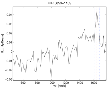
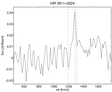
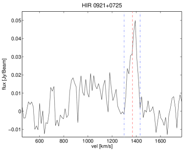
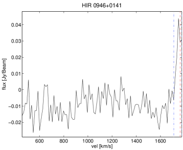
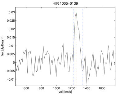
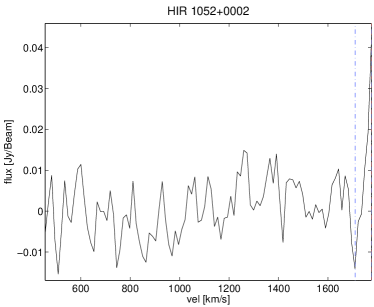
Figure 2: Spectra of new H i detections obtained from reprocessed HIPASS data. The radial velocity of each object is indicated by the red dashed vertical, the velocity width is indicated by the blue dash-dotted line.

Fig 2. (continued)

Fig 2. (continued)

4.5 Flux densities

The total flux densities have been determined for all detections using two independent methods. The line-widths and the integrated line-strengths have first been determined by integrating the brightness over the full velocity width of an object along the single spectrum that contains the overall peak brightness. We assume that all sources are unresolved and fully contained within the 15.5 arcmin beam. In a second approach the total flux has been determined from the integrated moment maps. Moment maps are created by collapsing the cube in the direction of the velocity axis over the full line width. The visualisation package KARMA (Gooch, 1996) has been used to integrate the flux. The radial profile of an object can be plotted, including a fit to the data points within a user defined circle. This circle was chosen to completely enclose the object, including any possible extended emission. The integrated flux densities have to be corrected for the beam integral to convert from Jy Beam^-1 km s^-1 to Jy km s^-1. An integrated flux density is determined by simply adding the pixels values, and a fitted flux density is determined by fitting a Gaussian to the radial profile. Since we aim to be sensitive to extended features that do not necessarily have a Gaussian profile, we use the pixel integral for our flux density determinations rather than a Gaussian fit.

When integrating the line strength of a single spectrum, not all the flux is measured if the source is resolved by the beam, or if there are extended emission features like filaments. The flux densities are plotted and compared in Fig. 3 where in the left panel the total flux obtained from the integrated pixel values is plotted as function of the single pixel integrated line strength. The dotted line goes through the origin and indicates where the fluxes are equal. Only those sources are plotted that are completely covered by our data cubes in both the spectral and spatial directions. The measured fluxes match the dotted line very well, meaning that there is typically no large discrepancy between the two different methods. The ratio of the fluxes is plotted on a logarithmic scale in the right panel of Fig. 3, the dotted line indicating again where the fluxes are equal. The mean of the ratios is 0.99, with a standard deviation of 0.28. The dashed line in the right panel of Fig. 3 represents the median of the flux ratios, which is 0.96. As both the mean and median values are close to one, there is generally very good agreement between the fluxes. For large flux values above $\sim 50$ Jy km s^-1 the fluxes derived by integrating the individual pixel values are typically larger by 20 to 50%. This is due to the fact that these are typically large and extended sources that are resolved by the beam. At low flux levels, there are a number of sources for which the integrated line-strength exceeds the integrated flux of the moment map by more than a factor of two. Since the line-strength of the peak spectrum provides a lower limit to the true integral, there must be a residual artefact in either the spectrum or the moment map. The spectra and moment maps of these sources were inspected and either the spectral bandpass appears slightly elevated, or there are negative residuals in the moment maps which influence the flux estimates.

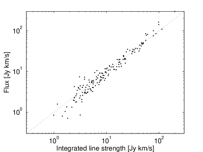
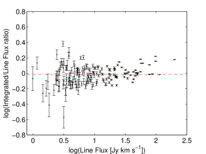
Figure 3: Left panel: Flux obtained from the moment maps is plotted as function of the line strength, the dotted line indicates where the two flux measurements are equivalent. Right panel: ratio of integrated flux and line-strength is plotted as function of line-strength on a logarithmic scale. The dotted line indicates where the ratio is one and the fluxes are equivalent. The dashed line shows the median of the ratios.

Another important comparison to make is of our measured fluxes with those obtained in the first HIPASS product. In Fig. 4 fluxes derived from the reprocessed HIPASS data are compared with fluxes in the HIPASS catalogue (Meyer et al., 2004; Wong et al., 2006). Again, only those sources are plotted that are completely covered by the data cubes. The left panel shows the reprocessed fluxes as function of original fluxes, while the right panel shows the ratio. The dashed line indicates the median of the flux ratios which is 1.10. The mean of the ratios is 1.31 with a standard deviation of 1.41. In this case the median estimate gives a better representation of the general trend instead of the mean, as the effect of strong outliers is suppressed.

The $\sim 10$% excess in flux in the published HIPASS product over that in our reprocessed result may reflect the variation in effective beam size with signal-to-noise ratio that is a consequence of median gridding, as discussed at some length in Barnes et al. (2001). Exactly the same data has been used in both processing methods, so another effect that may contribute to the difference in flux is how the bandpass is determined. The gridding of the data has been done in a similar fashion as for the original HIPASS product, so any differences are caused in the pre-gridding. For several sources the individual spectra in both the original and the re-reduced HIPASS product have been compared. Despite the difference in flux, the spectra look very similar. A difference in the fit to the bandpass can enhance the whole spectrum slightly, without significantly affecting the shape.

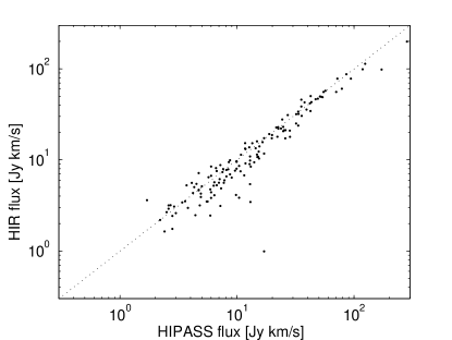
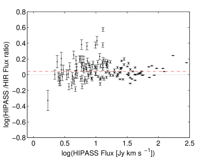
Figure 4: Left panel: The integrated line strength of the reprocessed HIPASS data (HIR) is plotted as function of the original HIPASS fluxes. Right panel: ratio of the first and reprocessed HIPASS product is plotted against the original HIPASS flux. The dashed line indicates where the fluxes are equal, while the dashed line represents the median of the ratios. On average there is a small excess in the flux values of the original HIPASS product.

4.6 Companions

Moment maps have been generated for all detected objects by integrating over their velocity widths. Initially, maps of 2 by 2 degrees in size are generated, to completely cover the detection itself, including the nearby environment. All moment maps were inspected by eye for diffuse emission features. For objects that showed tentative signs of filaments or companions, another moment map was generated of 5 by 5 degrees in size. These moment maps were inspected in detail, by searching for local peaks in the spatial domain as well as possible line features in the spectrum at the relevant velocity.

Several faint features have been marginally detected, that have not emerged from our earlier source finding procedure. These detections appear very interesting but would need further confirmation to make them robust. They are usually very faint, but some of them have very broad line-widths. None of the features have an optical counterpart, therefore the origin of the features is not straightforward. All of these tentative detections were found by visually inspecting the moment maps around bright sources. As none of them passed the criteria of previous source finding algorithms, it is very likely that a significant number of comparable features are still present in the data. We will discuss the detailed properties of all features below. The relevant spectra are shown in Fig. 5. A third order polynomial was fit to the spectrum, excluding the line itself and galactic emission, to correct for bandpass instabilities at these very low flux values. We will leave statements about the possible origin of these features to the discussion.

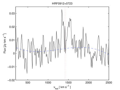
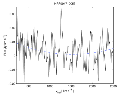
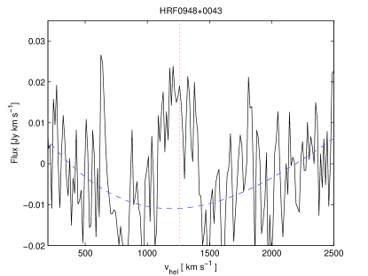
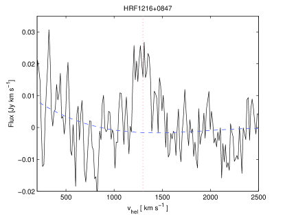
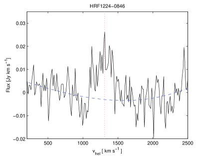
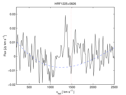
Figure 5: Spectra of H i features that have been detected in the vicinity of other objects, by inspecting the moment maps. A third order polynomial is fit to the bandpass and is indicated by the dashed line. The vertical dotted line represents the radial velocity of the detected feature.

Fig 5. (continued)

HIRF 0912+0723: The position of this feature, at RA=09:12:55 and DEC=07:23:34, is close to UGC 4781 and NGC 2777 and it has a comparable radial velocity to these galaxies of 1458 km s^-1. The spectrum has two peaks, that are separated by 140 km s^-1. The two peaks are reminiscent of a double horned profile, although they may simply be due to two unrelated structures within the telescope beam. A direct relation to either of the two cataloged galaxies is not obvious, as the line is quite broad and has a very different character. The total line integral at the indicated position is 3.9 Jy km s^-1, after correction of the spectral baseline. With an integrated signal-to-noise of $\sim 7$, this detection has moderately high significance.

HIRF 0947-0053 : This feature with RA=09:47:11 and DEC=-00:53:05 is near the optical source SDSS J094446.23-004118.2, in the same field as the previous detection. In contrast to HIRF 0948+0043, this detection is relatively narrow, with a $W_{20}$ value of 77 km s^-1 and it has one peak with a maximum brightness of $\sim 33$ mJy beam^-1. The integrated line-strength is only 1.3 Jy km s^-1, yielding a marginally significant signal-to-noise of 5.

HIRF 0948+0043: This feature is located at RA= 09:48:32 and DEC=00:43:23, offset by several degrees from NGC 3044 which has a consistent radial velocity of 1289 km s^-1. This is a very broad profile with a $W_{20}$ value of $\sim 320$ km s^-1. Although the brightness in each channel is only about 10 mJy Beam^-1, this brightness is present over 25 channels, which yields a high significance. The line-integral without any further smoothing is 7.6 Jy km s^-1, which corresponds to a signal to noise of 13. Intriguingly, there appear to be additional filamentary features in the field of this object. Similar broad line profiles can be recognised at several positions along the filament, albeit with low signal-to-noise. A DSS image of the region around HIRF 0948+0043 is shown in Fig. 6, which is indicated by the letter C in this image. The main galaxy in the top left of the plot is NGC 3044 which has extended emission. Letters B, C and D are assigned to regions in the environment showing emission. The line profiles are shown in Fig. 7, although the fluxes in all the companions are very low, they all have a line-width that is very comparable to NGC 3044. It appears as if these denser regions form a more extended filament. In Lee & Irwin (1997) a high resolution H i image of NGC3044 obtained with the VLA is presented. Although the brightness sensitivity of these observations is much lower than the Parkes data, at column density levels of a few times $N_{HI}\sim 10^{20}$ cm^-2 small companions can be seen in the same direction as the companions we detect.

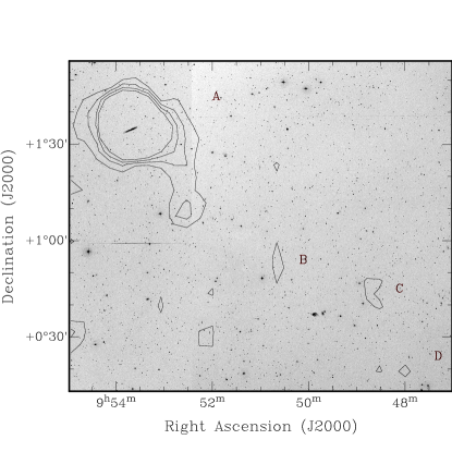
Figure 6: Second generation DSS image with H i contours at 2, 3, 4 and 5 Jy beam^-1 km s^-1. The large galaxy is NGC 3044, three companions are identified with very similar line-widths. The line profile of each object is shown in Fig. 7.

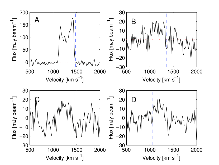
Figure 7: Line profiles of NGC 3044 (A) and three faint detection (B, C, D) in the extended environment of the galaxy.

HIRF 1216+847: At RA=12:16:45 and DEC=08:47:22 this detection has a radial velocity of 1299 km s^-1 and $W_{20}$=199 km s^-1. Although the peak brightness is not very substantial; $\sim 20$ mJy beam^-1 over the full line width, the integrated flux of 4.3 Jy km s^-1 corresponds to a signal-to-noise of 9.

HIRF 1224+0846: With an RA of 12:24:52 and DEC of 08:46:25, this detection is within half a degree of NGC 4316. The radial velocity of 1312 km s^-1 matches that of NGC 4316 fairly well. Of particular note is the very broad line-width of approximately 400 km s^-1. While the peak brightness is modest; only 24 mJy beam^-1 it extends quite uniformly across the entire line-width. This yields an integrated flux of 5.3 Jy km s^-1 corresponding to a signal-to-noise of 9.

HRIF 1225+0826: Located at RA=12:25:40 and DEC=08:26:16, this intriguing feature’s properties are very sensitive to the method of baseline definition. The overlaid baseline fit results in a central radial velocity of 1484 km s^-1, an integrated flux of 8.4 Jy km s^-1, an extremely broad line-width of about 700 km s^-1 at 20% of the peak flux and a signal-to-noise of 10. However, other spectral baselines would severely diminish the apparent line-width, flux and overall significance of this feature. A slightly enhanced baseline fit would also cut the source in half, therefore potentially this detection could also consist of two different sources with a different spectral position within the telescope beam. Confirming observations will be necessary to establish it’s reliability.

HRIF 1230+0949: This is a very similar detection to several of those discussed previously, with a low peak brightness, but a very broad line-width. This objects is located at RA=12:30:24 and DEC=09:49:45 with a radial velocity of 1180 km s^-1. The integrated flux of 3.7 Jy km s^-1 over a line-width $W2_{20}$ of 280 km s^-1, yield a signal-to-noise of 7.

HIRF 1257+0407: This detection at RA=12:57:20 and DEC=04:07:59 is in the direct environment of NGC 4804 with a radial velocity of 824 km s^-1 that is comparable to this galaxy. The peak flux of 35 mJy beam s^-1 is relatively strong, compared to the other detections listed here. The line-width at 20% of the peak is 102 km s^-1 and the integrated flux of 2.4 Jy km s^-1 has a signal-to-noise of 7.

HIRF 1323+0206: This detection is at RA= 13:23:17 and DEC=02:06:06, with a radial velocity of 980 km s^-1. This is another example of a very faint source with a very broad line width of more than 500 km s^-1. The brightness in each individual channel barely exceeds the $1\sigma$ level. The line-width at 20% of the peak is 505 km s^-1 and the integrated line strength is 5.2 Jy km s^-1, which corresponds to a signal-to-noise of 7.

HIRF 1334+0810: This detection at RA=13:34:21 and DEC=08:10:14 is only marginal. The peak brightness is $\sim 25$ mJy beam^-1 and the integrated flux is 2.2 Jy km s^-1 and has a signal to noise of only 6.5 when taking into account the $W_{20}$ of 110 km s^-1. Interesting however is that this feature is about half a degree south of an extended chain of galaxies that is connected to NGC 5248 in the data. Although these galaxies individually could not be resolved in the HIPASS data, optical images from DSS can reveal UGC 8575 and CGCG 073-036. Both these galaxies and HIRF 1324+0810 have a similar radial velocity of $\sim$1200 km s^-1 and a narrow line profile that is completely embedded in the profile of NGC 5248. This diffuse detection seems to be connected to the filament of galaxies, although the connecting bridge is very faint.

4.7 Completeness and Robustness

Our source catalogue has been constructed from all sources which have a peak brightness exceeding our 5$\sigma$ limit of $\sim$50 mJy beam^-1 at “full” velocity resolution of 26 km s^-1 and correspondingly fainter brightnesses after velocity smoothing to 52 and 104 km s^-1. Simulations involving the injection of artificial sources into similar total power H i data-cubes by Rosenberg & Schneider (2002) have shown that an asymptotic completeness of about 90% is reached at a signal-to-noise ratio of 8, while the completeness at a signal-to-noise ratio of 5 is only likely to be about 30%.

We have used the Duchamp (Whiting, 2008) source finding tool to find candidate sources in the data cubes at the different velocity resolutions. The source finder was found to be robust down to this 5$\sigma$ limit on peak brightness. All candidate sources were subsequently inspected visually. Artefacts from solar interference or due to bright continuum sources could easily be rejected. A lower threshold for the source finder resulted in a much larger proportion of candidates that were deemed unreliable after visual inspection. Moment maps of all candidate detections have been further inspected and analysed interactively resulting in some additional detections of interesting features. As these features were sought preferentially in the direct vicinity of other galaxies, they have not been cataloged to the same level of completeness throughout the data volume. Although many of these features appear highly significant, their derived properties are often quite sensitive to the form of the spectral baseline that is subtracted.

We have found two classes of objects. The first ones are relatively narrow lines, with a total line width of $\sim 100$ km s^-1 or a FWHM of $\sim 50$ km s^-1 and a peak brightness per 26 km s^-1 velocity channel that only exceeds the local noise by a factor three or four. The second class of objects has very broad line widths of up to $\sim 500$ km s^-1, however the measured brightness per line channel only exceeds the local noise by a factor two, or not at all. Because of the broad line widths, the integrated detections have a high significance, but such features are particularly difficult to detect with an automatic source finder. Although the detections seem significant, they need further confirmation as the nature and broad line-width of these objects is unexpected. Nevertheless it seems unlikely that these detections are an artefact of the reduction pipeline or the method of bandpass estimation. Only a second order polynomial has been fit to the bandpass in each spectrum. For most of the broad lines, a range of channels is systematically elevated above the rest of the spectrum and the transition is quite sharp. Higher order polynomials would be needed to artificially create such features.

5 Discussion

In this paper we describe how a significant part of the raw HIPASS observations have been reprocessed. The reprocessed region covers the right ascension range from 8 to 17 hours and Declinations from -1 to 10 degrees. A source catalogue and H i features without optical counterparts have been presented. Although the original HIPASS product is an excellent one in its own right, by improving the reduction and processing pipeline the quality and number of detections can be significantly improved. The main purpose of reprocessing this particular region is because of the overlap with the WVFS survey as described in Popping & Braun (2011a) and Popping & Braun (2011b) and the HIPASS data complements the two data products of the WVFS survey. The first WVFS product has a worse flux sensitivity than the HIPASS data, but a better column density sensitivity due to the very low resolution of this dataset. On the opposite the second WVFS product has a better flux sensitivity than the HIPASS data, but a worse column density sensitivity as the resolution of this data is higher than the resolution of the Parkes telescope.

We will leave detailed analysis and discussion to a later paper, when the three independent datasets will be compared. A few comments will be made that are relevant to this dataset and these detections.

5.1 Red-shifted OH

There are several detections, both in the source list, as well as identified as possible filaments, that do not have an optical counterpart. Because there is no optical counterpart, the origin of these features is not straightforward. All detections were considered to be H i detections that could reside in the vicinity of other objects as tidal remnants or Cosmic Web features. Another scenario that has not been explored is red-shifted OH emission from sources at a redshift of $z\sim 0.15$. The 1665.401/1667.358 MHz doublet of an OH megamaser emitted at this redshift would have an observed frequency of $\sim 1415$ MHz. Although confirmed detections of these red-shifted OH megamasers have not yet been reported, they are predicted to be found in blind H i surveys . ALFALFA (Giovanelli et al., 2005) expects to find several dozen OHMs in the redshift interval 0.16-0.25. Although the area covered by ALFALFA is significantly larger, based on these numbers we can expect to detect a few OHMs in our survey volume. To detect the OH doublet, two similar peaks should be identified with a separation of $\sim 350$ km s^-1. When looking at the profiles of known OHMs in e.g. Darling & Giovanelli (2002), the doublet is not always clearly apparent and so this requirement might be somewhat relaxed. All the documented OHMs do have a broad line-width, typically larger than 300 km s^-1. This consideration rules out most of our detections without optical counterparts as candidate OHMs, as the line-widths are much narrower. There are however a few cases, where this may be a possible scenario, namely: HRF 0948+0043, HRF 1224+0846, HRF 1225+0826 and HRF 1323+0206. The other prediction of this scenario is that a suitable ULIRG at $z\sim 0.15$ should be coincident with the $\sim$1415 MHz line detection. We have sought for objects at the appropriate redshift that coincide with the spatial positions of these detections, but did not find any sources that could cause redshifted OH emission.

5.2 Gas accretion modes

An interesting question regarding structure formation is how the intergalactic medium fuels the galaxies; ie. how gas is accreted. The two most discussed scenarios are hot mode and cold mode accretion (Kereš et al., 2005). The line-width of a detection can be used to estimate the upper limit of the kinetic temperature of the gas and is given by:

$$T_{kin}\leq\frac{m_{H}\Delta V^{2}}{8k\ln 2}$$ (4)

where $m_{H}$ is the mass of an hydrogen atom, $k$ is the Boltzmann constant and $\Delta V$ is the H i line-width at FWHM. This equation gives an upper limit to kinetic temperature, as internal turbulence or rotation can also increase the line-width of an object.

In the case of cold mode accretion with temperatures of the order of $T<10^{5}$ K, the line-widths of the gas are relatively narrow, up to $\sim 100$ km s^-1. The conditions to observe such gas are relatively easily satisfied, the neutral fraction in cold gas is still significant so that the H i column density is still high. Although it is difficult to distinguish tidal remnants from pristine gas that is fuelling the galaxies, gas accretion is a very plausible scenario. The details of our detections will be discussed later when other data products are included. There are however a handful of detections in the direct vicinity of other galaxies that are not bright, but have line-widths up to $>500$ km s^-1. One possible scenario is that this is red-shifted OH emission as is discussed in the previous subsection, but this is very unlikely. These line-widths are however also the line-widths that are expected in the case of hot-mode-accretion. This is gas that is gradually shock heated during structure formation to virial temperatures and than rapidly cools down to accrete onto the galaxies, for a more extended explanation see Kereš et al. (2005). Because this gas is highly ionised, the neutral fraction is very low, so the H i component of such gas is extremely small and very unlikely.

6 Conclusion

Original data of the H i Parkes All Sky Survey has been reprocessed, that overlaps in sky coverage with the Westerbork Virgo Filament Survey. This region was selected to complement the WVFS and use HIPASS to confirm candidate detections. Furthermore, HIPASS is an excellent dataset, to search for diffuse H i features that can be related to the neutral component of the Cosmic Web.

By using an improved reduction strategy, we achieved a reduced RMS value and lower artefact level, compared to the original HIPASS product. In the reprocessed data, we achieve a noise value of $\sim 10$ mJy beam^-1 over 26 km s^-1, which is a $\sim 20$% improvement over the original HIPASS product. The data has a $1\sigma$ brightness sensitivity of $\sim 3.5\cdot 10^{17}$ cm^-2, which allows direct detection in H i emission of some of the higher column density Lyman Limit Systems seen in QSO absorption line studies.

The major difference with respect to the original HIPASS cubes is that negative artefacts in the bandpass in the vicinity of bright sources are almost completely eliminated. This allows us to search for diffuse and extended H i emission, which has not been possible before.

In total we have detected 203 objects in the reprocessed region, of which 29 had not been catalogued in the original HIPASS source catalogue. Fourteen of these detections are completely new H i detections, of which many do not have an optical counterpart. Although these detections are briefly mentioned, detailed discussion and possible confirmation from other data sets will be presented in a subsequent paper in this series.

In this work only a relatively small part of the HIPASS data has been reprocessed, as that survey covers the complete Southern sky and the Northern sky up to +24 degrees in Declination. Apart from this work, steps have been undertaken to further improve the reduction pipeline and reprocess the complete survey area. Improved data cubes, together with improved object-searching algorithms will permit detection of significantly more sources. This will provide improved statistics on the distribution of H i in the local universe. The reprocessed cubes will also permit an unbiased search for diffuse neutral hydrogen and Cosmic Web filaments, although currently there is no other all-sky H i survey with an appropriate brightness sensitivity and distinct angular resolution to complement this data.

Appendix A Spectra H i detections in the reprocessed H i Parkes All Sky Survey data.

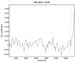
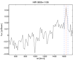
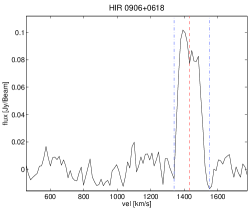
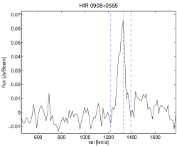
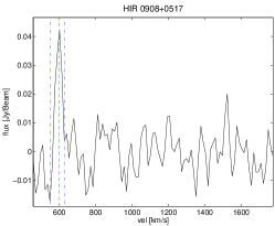
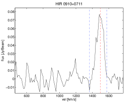
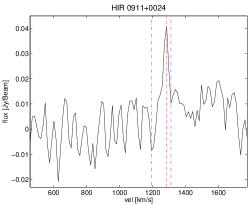
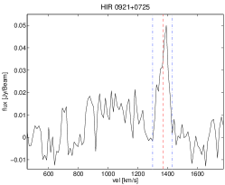
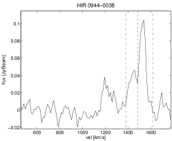
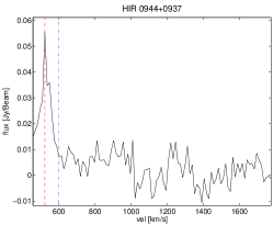
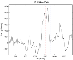
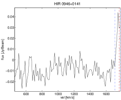
Figure 8: Spectra of all detections of neutral hydrogen in the reprocessed region of the H i Parkes All Sky Survey. The velocity width of each object is indicated by the two blue dash-dotted lines, while the central velocity is shown by the red dashed line.

Fig 8. (continued)

Fig 8. (continued)

Fig 8. (continued)

Fig 8. (continued)

Fig 8. (continued)

Fig 8. (continued)

Fig 8. (continued)

Fig 8. (continued)

Fig 8. (continued)

Fig 8. (continued)

Fig 8. (continued)

Fig 8. (continued)

Fig 8. (continued)