Quantum correlations in the thermodynamic limit: the XY-model

Abstract

We investigate thermal properties of quantum correlations in the thermodynamic limit with reference to the XY-model

Keywords: Quantum Entanglement, Quantum Discord

I Introduction

Since the formalization by Werner W89 of the modern concept of quantum entanglement it has become clear that there exist entangled states that comply with all Bell inequalities (BI). This entails that non-locality, associated to BI-violation, constitutes a non-classicality manifestation exhibited only by just a subset of the full set of states endowed with quantum correlations. Later work by Zurek and Ollivier olli established that not even entanglement captures all aspects of quantum correlations. These authors introduced an information-theoretical measure, quantum discord, that corresponds to a new facet of the “quantumness” that arises even for non-entangled states. Indeed, it turned out that the vast majority of quantum states exhibit a finite amount of quantum discord.

The tripod non-locality-entanglement-quantum discord is of obvious interest and possesses technological implications. The crucial role played by quantum entanglement in quantum information technologies is well known Nielsen . In some cases, however, entangled states are useful to solve a problem if and only if they violate a Bell inequality comcomplex . Moreover, there are important instances of non-classical information tasks that are based directly upon non-locality, with no explicit reference to the quantum mechanical formalism or to the associated concept of entanglement device . Last, but certainly not least, recent research indicates that quantum discord is also a valuable resource for the implementation of non-classical information processing protocols geom ; ferraro ; dattaprl ; luo ; datta . On the light of these developments, it becomes imperative to conduct a systematic exploration of the connections between the tripod members.

We investigate here the relation between quantum discord and entanglement and in an infinite system, namely, the XY model in the thermodynamic limit LSM . This model, like the celebrated Ising and Heisenberg models, is one of the paradigmatic systems in statistical mechanics. The Hamiltonian of the anisotropic one-dimensional spin-$\frac{1}{2}$ XY model in a transverse magnetic field $h$ ($N$ particles) reads

$$H=\sum_{j=1}^{N}[(1+\gamma)S_{x}^{j}S_{x}^{j+1}+(1-\gamma)S_{y}^{j}S_{y}^{j+1}]-h\sum_{j=1}^{N}S_{z}^{j},$$ (1)

where $\sigma^{j}_{u}=2S_{u}^{j}$ ($u=x,y,z$) are the Pauli spin-$\frac{1}{2}$ operators on site $j$, $\gamma\in[0,1]$ and $\sigma^{j+N}_{u}=\sigma^{j}_{u}$. The model (1) for $N=\infty$ is completely solved by applying a Jordan-Wigner transformation LSM ; Barouch , which maps the Pauli (spin 1/2) algebra into canonical (spinless) fermions. The system (except for the isotropic case $\gamma=0$) undergoes a paramagnetic-to-ferromagnetic quantum phase transition (QPT) qpt ; Sachdev driven by the parameter $h$ at $h_{c}=1$ and $T=0$. It is well known that near factorization a characteristic length scale naturally emerges in the system, which is specifically related with the entanglement properties and diverges at the critical point of the fully isotropic model baroni .

It is thus our intention in this communication to study the interplay of entanglement and quantum discord for the XY model in the thermodynamic limit. To such an effect we will consider in Section II the correlations existing between a pair of qubits located at two given sites. For comparison purposes we shall also discuss in Section III the correlations between pairs of qubits in the finite Heisemberg model. Some conclusions are drawn in Section IV.

I.1 Quantum discord

Quantum discord geom ; olli constitutes a quantitative measure of the “non-classicality” of bipartite correlations as given by the discrepancy between the quantum counterparts of two classically equivalent expressions for the mutual information. More precisely, quantum discord is defined as the difference between two ways of expressing (quantum mechanically) such an important entropic quantifier. Let $\rho$ represent a state of a bipartite quantum system consisting of two subsystems $A$ and $B$. If $S(\rho)$ stands for the von Neumann entropy of matrix $\rho$ and $\rho_{A}$ amd $\rho_{B}$ are the reduced (“marginal”) density matrices describing the two subsystems, the quantum mutual information (QMI) $M_{q}$ reads olli

$$M_{q}(\rho)=S(\rho_{A})+S(\rho_{B})-S(\rho).$$ (2)

This quantity is to be compared to another quantity ${\tilde{M}}_{q}(\rho)$, expressed using conditional entropies, that classically coincides with the mutual information. To define ${\tilde{M}}_{q}(\rho)$ we need first to consider the notion of conditional entropy. If a complete projective measurement $\Pi_{j}^{B}$ is performed on B and (i) $p_{i}$ stands for $Tr_{AB}\,\Pi_{i}^{B}\,\rho$ and (ii) $\rho_{A||\Pi_{i}^{B}}$ for $[\Pi_{i}^{B}\,\rho\,\Pi_{i}^{B}/p_{i}]$, then the conditional entropy becomes

$$S(A|\,\{\Pi_{j}^{B}\})=\sum_{i}\,p_{i}\,S(\rho_{A||\Pi_{i}^{B}}),$$ (3)

and ${\tilde{M}}_{q}(\rho)$ adopts the appearance

$${\tilde{M}}_{q}(\rho)_{\{\Pi_{j}^{B}\}}=S(\rho_{A})-S(A|\,\{\Pi_{j}^{B}\}).$$ (4)

Now, if we minimize over all possible $\Pi_{j}^{B}$ the difference $M_{q}(\rho)-{\tilde{M}}_{q}(\rho)_{\{\Pi_{j}^{B}\}}$ we obtain the quantum discord $\Delta$, that quantifies non-classical correlations in a quantum system, including those not captured by entanglement. One notes then that only states with zero $\Delta$ may exhibit strictly classical correlations. Among many valuable discord-related works we just mention two at this point that are intimately related to the present one, e.g., those of Zambrini et al. zambrini and Batle et al. ours .

II Two qubits in the infinite $XY$ model

The general two-site density matrix is expressed as

$$\rho_{ij}^{(R)}=\frac{1}{4}\,\Bigg{[}I+\sum_{u,v}T_{uv}^{(R)}\sigma^{i}_{u}\otimes\sigma^{j}_{v}\Bigg{]}.$$ (5)

$R=j-i$ is the distance between spins, $\{u,v\}$ denote any index of $\{\sigma_{0},\sigma_{x},\sigma_{y},\sigma_{z}\}$, and $T_{uv}^{(R)}\equiv\langle\sigma^{i}_{u}\otimes\sigma^{j}_{v}\rangle$. Due to symmetry considerations, only $\{T_{xx}^{(R)},T_{yy}^{(R)},T_{zz}^{(R)},T_{xy}^{(R)}\}$ do not vanish. Barouch et al Barouch have provided exact expressions for two-point quantum correlations, together with details of the dynamics associated with an external field $h(t)$. For the purposes of this paper, we will consider only systems which at time $t=0$ are in thermal equilibrium at temperature $T$. We have then the canonical ensemble expression $\rho(t=0)=\exp{[-\beta\,H]}$, where $\beta=1/kT$ and $k$ is the Boltzmann constant. Following Barouch , one obtains $T_{xx}^{(1)}=G_{-1},T_{yy}^{(1)}=G_{1},T_{zz}^{(1)}=G_{0}^{2}-G_{1}G_{-1}-S_{1}S_{-1}$, and $T_{xy}^{(1)}=S_{1}$, where

$$G_{R} = \frac{\gamma}{\pi}\int_{0}^{\pi}d\phi\sin(R\phi)\frac{\tanh\big{[}\frac{1}{2}\beta\Lambda(h_{0})\big{]}}{\Lambda(h_{0})\Lambda^{2}(h_{f})}$$ (11)

$$\times[\gamma^{2}\sin^{2}\phi+(h_{0}-\cos\phi)(h_{f}-\cos\phi)$$

$$-(h_{0}-h_{f})(h_{f}-\cos\phi)\cos(2\Lambda(h_{f})t)]$$

$$-\frac{1}{\pi}\int_{0}^{\pi}d\phi\cos(R\phi)\frac{\tanh\big{[}\frac{1}{2}\beta\Lambda(h_{0})\big{]}}{\Lambda(h_{0})\Lambda^{2}(h_{f})}$$

$$\times\big{[}\{\gamma^{2}\sin^{2}\phi+(h_{0}-\cos\phi)(h_{f}-\cos\phi)\}(\cos\phi-$$

$$h_{f})-(h_{0}-h_{f})\gamma^{2}\sin^{2}\phi\cos(2\Lambda(h_{f})t)],$$

$$S_{R} = \frac{\gamma(h_{0}-h_{f})}{\pi}\int_{0}^{\pi}d\phi\sin(R\phi)\sin\phi\frac{\sin[2\Lambda(h_{f})t]}{\Lambda(h_{0})\Lambda(h_{f})},$$ (13)

with $\Lambda(h)=[\gamma^{2}\sin^{2}\phi+(h-\cos\phi)^{2}]^{1/2}$. $G_{R}$ is the two-point correlator appearing in the pertinent Wick-calculations and $M_{z}=\frac{1}{2}G_{0}$. The two-spin correlation functions are given by Barouch

$$\langle\sigma_{x}^{i}\sigma_{x}^{i+R}\rangle =\begin{vmatrix}G_{-1}&G_{-2}&\cdots&G_{-R}&\\ G_{0}&G_{-1}&\cdots&G_{-R+1}&\\ \vdots&\vdots&\ddots&\vdots&\\ G_{R-2}&G_{R-3}&\cdots&G_{-1}&\end{vmatrix},$$ (14)

$$\langle\sigma_{y}^{i}\sigma_{y}^{i+R}\rangle =\begin{vmatrix}G_{1}&G_{0}&\cdots&G_{-R+2}&\\ G_{2}&G_{1}&\cdots&G_{-R+3}&\\ \vdots&\vdots&\ddots&\vdots&\\ G_{R}&G_{R-1}&\cdots&G_{1}&\end{vmatrix},$$ (15)

$$\langle\sigma_{z}^{i}\sigma_{z}^{i+R}\rangle =4\langle\sigma_{z}\rangle^{2}-G_{R}G_{-R},$$ (16)

where $R=j-i$ (distance between spins). In the case where more than two particles are considered, the previous correlators no longer possess their previous Toeplitz matrix structure Batle2010 .

It will prove convenient to cast the two qubit states (5) in two forms. States $\rho_{ij}^{(R)}$ are written in the computational basis $\{|00\rangle,|01\rangle,|10\rangle,|11\rangle\}$ as

$$\frac{1}{4}\left(\begin{array}[]{cccc}1+4M_{z}+T_{zz}&0&0&T_{xx}-T_{yy}-i2T_{xy}\\ 0&1-T_{zz}&T_{xx}+T_{yy}&0\\ 0&T_{xx}+T_{yy}&1-T_{zz}&0\\ T_{xx}-T_{yy}+i2T_{xy}&0&0&1-4M_{z}+T_{zz}\end{array}\right).$$ (17)

These very states $\rho_{ij}^{(R)}$ acquire instead the following form in the Bell basis $\{|\Phi^{+}\rangle,|\Phi^{-}\rangle,|\Psi^{+}\rangle,|\Psi^{-}\rangle\}$

$$\left(\begin{array}[]{cccc}\rho_{11}&i\rho^{I}_{12}&i\rho^{I}_{13}&\rho^{R}_{14}\\ -i\rho^{I}_{12}&\rho_{22}&\rho^{R}_{23}&i\rho^{I}_{24}\\ -i\rho^{I}_{13}&\rho^{R}_{23}&\rho_{33}&i\rho^{I}_{34}\\ \rho^{R}_{14}&-i\rho^{I}_{24}&-i\rho^{I}_{34}&\rho_{44}\end{array}\right).$$ (18)

This special form is such that one can use it to analytically compute the maximal violation of a Bell inequality, a measure for nonlocality Batle2010 . In turn states $\rho_{ij}^{(R)}$ in (17) are of such special aspect that the quantum discord Qd turns out to be to be analytically given (see Ref. rossig ). Nevertheless, the concomitant Qd can be easily obtained, in different fashion, as follows. The most general parameterization of the local measurement that can be implemented on one qubit (let us call it B) is of the form $\{\Pi_{B}^{0^{\prime}}=I_{A}\otimes|0^{\prime}\rangle\langle 0^{\prime}|,\Pi_{B}^{1^{\prime}}=I_{A}\otimes|1^{\prime}\rangle\langle 1^{\prime}|\}$. More specifically we have

$$|0^{\prime}\rangle \leftarrow \cos\alpha|0\rangle+e^{i\beta^{\prime}}\sin\alpha|1\rangle$$ (19)

$$|1^{\prime}\rangle \leftarrow e^{-i\beta^{\prime}}\sin\alpha|0\rangle-\cos\alpha|1\rangle,$$ (20)

which is obviously a unitary transformation –rotation in the Bloch sphere defined by angles $(\alpha,\beta^{\prime})$– for the B basis $\{|0\rangle,|1\rangle\}$ in the range $\alpha\in[0,\pi]$ and $\beta^{\prime}\in[0,2\pi)$. After some cumbersome calculations, it turns out that the expression for a minimum discord $\Delta$ of the Introduction exhibits a positive and nonsingular Hessian, convex for the relevant range of values of $(\alpha,\beta^{\prime})$. Our expression possesses thus a unique global minimum, that occurs when the concomitant partial derivatives vanish. This happens whenever we have $(\sin\alpha=\frac{\sqrt{2}}{2},\sin\beta^{\prime}=0)$.

The present results correspond to pairwise entanglement and quantum discord for the infinite $XY$ model at any temperature, including zero-one. This implies that one does not really need to “solve” the model in the sense of sufficiently augmenting the number of spins in the chain for the results to be thermally relevant. $T$ here is an actual, thermometer-measurable temperature, since we are tackling a “real” thermodynamic system. This is to be confronted to the vast XY-literature associated to finite spin-numbers, where $T$ is not, strictly speaking, well-defined in the thermodynamics sense.

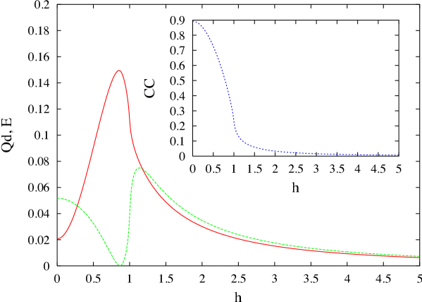
Figure 1: Color online) Plot of quantum discord Qd (upper solid curve) and entanglement of formation E (lower dashed curve) vs the external magnetic field $h$ for two qubits in infinite the $XY$ model (nearest neighbors), with anisotropy $\gamma=\frac{1}{2}$ at T=0. The region around the factorizing field $h_{f}$ concentrates maximum Qd. Inset depicts the corresponding classical correlations CC vs $h$. See text for details.

A comparison between the discord Qd and the entanglement of formation $E$ at $T=0$ is displayed in Fig. 1 (from now on we shall take the Boltzmann constant $k=1$). Qd and $E$ are depicted versus the external magnetic field $h$ (anisotropy $\gamma=\frac{1}{2}$) for the nearest neighbor configuration $R=1$. Remarkably enough, the Qd measure exhibits a maximum in the vicinity of the factorizing field $h_{f}=\sqrt{1-\gamma^{2}}$. Both Qd and $E$ seem to decay in the same fashion. The classical correlations (CC) for the same configuration are depicted in the inset of Fig. 1. Notice that all quantities here considered, i.e., Qd, $E$, or CC, are ultimately described in terms of several $G_{R}$s for all configurations, so that they all diverge at the QPT (for $h=1$) in the same way.

As an illustration consider the magnetization given by $M_{z}(h)=\frac{1}{2}G_{0}=\frac{\partial}{\partial h}\frac{1}{2\pi}\int_{0}^{\pi}d\phi[\gamma^{2}\sin^{2}\phi+(h-\cos\phi)^{2}]^{1/2}$. For $\gamma=1$ we have $M_{z}(h)=\frac{\partial}{\partial h}\big{(}\frac{2(h+1)}{2\pi}E\big{[}\frac{2\sqrt{h}}{h+1}\big{]}\big{)}=\frac{1}{2\pi}\big{[}\frac{h-1}{h}K\big{(}\frac{2\sqrt{h}}{h+1}\big{)}+\frac{h+1}{h}E\big{(}\frac{2\sqrt{h}}{h+1}\big{)}\big{]}$, where $K(E)$ is the complete elliptic integral of the first(second) kind. Since $\frac{d}{dh}M_{z}$ diverges in logarithmic way at $h=1$, as also do the divergence of $K$ and the first derivatives of $E$, Qd, and CC. In other words, they all signal the presence of a $h=1$-QPT at zero temperature (except for the isotropic case $\gamma=0$). In fact, the possibility of detecting a QPT at finite $T$ by using Qd has been recently considered by Werlang et al. Werlang . They perfom an interesting analysis of the role of the temperature and Qd in several quantum systems. We remember that a different concept such as nonlocality –as measured by the maximum violation of the well known Clauser-Horne-Shimony-Holt Bell inequality– was also considered as a QPT in Batle2010 (also in the context of the XY-model). In the present work we do not focus attention on this particular issue of QPTs, but study instead the comparison between entanglement and quantum discord for finite and infinite systems at non-zero temperature.

Fig. 2 depicts the the same quantities as Fig. 1 for several configurations. As we increase the relative distance from $R=1$ to 2, 3, and $\infty$, the corresponding Qd’s diminishes and also decays in faster and faster fashion with $h$. Notice that while entanglement (not shown here) globally diminishes, Qd only tends to vanish for $h>1$ and $R=\infty$. The inset here depicts the CC for the same configurations. They decreasing in the same fashion. While $E$ tends to zero, both Qd and CC remain nonzero, regardless of the distance between spins along the infinite chain.

As soon as we introduce a non-zero temperature things drastically change. In Fig. 3 we display several quantities at different temperatures ($T=0.01,0.1,0.3,0.5,1$): $R=1$ and $\gamma=\frac{1}{2}$. Fig. 3(a) depicts the entanglement of formation $E$ for states $\rho_{ij}^{(R)}$ (5) versus the magnetic field $h$ as we increase the temperature. $T$ lowers and broadens the region of null entanglement from a point at the factorizing field $h_{f}$ ($T=0$) to finite intervals centered at $h_{f}$. Eventually, $E$ becomes finite at higher values of $h$. This temperature-generated entanglement is depicted quantitatively in Fig. 3(b), where the region of zero entanglement extends from a point at zero $T$ to a finite-sized region as $T$ grows. The aforementioned region ceases to be finite beyond a critical temperature that depends on the particular $R$’s and $\gamma$’s involved therein. We discern some resemblance with a phase diagram: within the area encompassed by the two curves of Fig. 3(b) no entanglement is detected. It is surprising that, for the whole region, Qd globally diminishes and tends to be concentrated in the null-$E$ region, as can be seen in Fig. 3(c). These facts allow one to readily appreciate how different is the behavior of entanglement vis-a-vis that of Qd. The role of classical correlations can be observed in Fig. 3(d). For the same set of temperatures employed above CC decreases i) as we augment $T$ and ii) for increasing values of $h$, a behavior different from that of entanglement: while CC never vanishes, it is larger wherever $E=0$. Both $E$ and CC coexist for high values of $h$. We are dealing with a system for which, as we increase the temperature, entanglement survives –although barely– for high values of $h$. This fact clearly affects the existence of finite discord- or CC-values. Recall that this was the case already at $T=0$. The role of the factoring field $h_{f}$ in defining higher or lower values of Qd becomes crucial. To further analyze the nontrivial relation between entanglement $E$ and quantum discord Qd at finite $T$ it would enlightening to consider a physical system for which $E$ would increase with the temperature. Such is the Heisenberg model’s scenario, also a statistical mechanical model used in the study of critical points and phase transitions of magnetic systems baxter ; Arnesen .

III Two qubits in the (finite) Heisenberg model

First of all note that because of its finitude the system is not immersed in an infinite thermal bath. Thus, we cannot stricto-sensu speak of a “temperature”. However, the results to be presented are illustrative of the intricacies of entanglement and quantum discord. Following the interesting work of Arnesen et al. Arnesen , we concern ourselves with the issue of thermal entanglement but extend the discussion so as to encompass thermal discord. The Hamiltonian for the 1D Heisenberg spin chain with a magnetic field of intensity $B$ along the $z$-axis reads

$$H\,=\,\sum_{i=1}^{N}(B\sigma^{i}_{z}\,+\,J_{H}\vec{\sigma}^{i}\,\vec{\sigma}^{i+1}),$$ (21)

where $\sigma^{i}_{x,y,z}$ stand for the Pauli matrices associated to the spin $i$. Periodic boundary conditions are imposed ($\sigma^{N+1}_{\mu}=\sigma^{1}_{\mu}$). $J_{H}$ is the strength of the spin-spin repulsive interaction (only the anti-ferromagnetic ($J_{H}>0$) instance is discussed). If we limit ourselves to the case $N=2$, we deal with two spinors, i.e., with a two-qubits system. So as to speak of “thermal equilibrium” we consider the thermal state Arnesen

$$\rho(T)=\frac{\exp(-\frac{H}{k_{B}T})}{Z(T)},$$ (22)

with $Z(T)$ the partition function. Expressing both $H$ and $\rho(T)$ in the computational basis $|00\rangle,|01\rangle,|10\rangle,|11\rangle$ we obtain

$$H=\left(\begin{array}[]{cccc}2J_{H}+2B&0&0&0\\ 0&-2J_{H}&4J_{H}&0\\ 0&4J_{H}&-2J_{H}&0\\ 0&0&0&2J_{H}-2B\end{array}\right).$$ (23)

After defining, for convenience’s sake,
$e_{wmy}=\exp{\,(-2w-2y)};$
$e_{wp}=\exp{\,(-2w)}+\exp{\,(6w)};$
$e_{wm}=\exp{\,(-2w)}-\exp{\,(6w)}$;
$e_{wpy}=\exp{\,(-2w+2y)},$
with $w=J_{H}/k_{B}T$ and $y=B/k_{B}T$, we also get

$$\rho(T)=\frac{1}{Z(T)}\left(\begin{array}[]{cccc}e_{wmy}&0&0&0\\ 0&e_{wp}/2&e_{wm}/2&0\\ 0&e_{wm}/2&e_{wp}/2&0\\ 0&0&0&e_{wpy}\end{array}\right),$$ (24)

In this case the concurrence of $\rho(T)$ reads Arnesen

$$C = 0;\,\,\,\,\,\,\,\,\,\,\,\,\,\,\,\,\,\,\,\,\,\,\,\,\,\,\,\,\,\,\,\,\,\,\,\,\,\,\,\rm{for}\,\,\,T\geq T_{c},$$ (25)

$$C = \frac{e^{8w}-3}{1+e^{-2y}+e^{2y}+e^{8w}};\,\,\rm{for}\,T<T_{c},$$ (26)

Recall that there is no entanglement beyond a certain critical temperature $T_{c}=8J_{H}/(k_{B}\ln 3)$ Arnesen , as can be seen from the previous $C-$computation. Also, there is a change in the structure of the ground state of hamiltonian (21) when the magnetic field reaches the critical value $B_{c}=4J_{H}$. In the limit of zero temperature, the ground state of the system may be represented by three different pure states: i) for $B<B_{c}$ (non-degenerate), the thermal state reduces to the singlet state $|\Psi^{-}\rangle\langle\Psi^{-}|$, ii) at $B=B_{c}$ (two-fold degenerate) $\frac{1}{2}|\Psi^{-}\rangle\langle\Psi^{-}|+\frac{1}{2}|11\rangle\langle 11|$, iii) whereas for $B<B_{c}$ (non-degenerate) we have $|11\rangle\langle 11|$. The previous $B-$distinctions are crucial in order to understand how the concomitant thermal state will respond to $T-$changes. We expect accompanying behaviors from $E$ and Qd whenever the initial state is pure (both quantities coincide in such case). Differences should emerge for $B>B_{c}$ whenever we study the unexpected behavior of increasing $E$ versus $T$ as far as Qd is concerned. The computation of Qd is in the present case analytic and corresponds to $\sin\alpha=\frac{\sqrt{2}}{2}$ for any $\beta$. The pertinent scenario is the subject of Fig. 4 (let us assume $J_{H}=1$, so that $B_{c}=4$). For the $B$-range of values that are smaller than the critical value $B_{c}$, entanglement, discord and CC all diminish as the $T$ increases, as shown in Fig. 4(a). This behaviour also occurs at $B=B_{c}$ and is depicted in Fig. 4(b). Notice in both cases the sudden death of entanglement, whereas the other quantities “survive” in indefinite fashion. Fig. 4(c) plots the same quantities for a magnetic field $B>B_{c}$. Remarkably enough, in this case entanglement as well as the quantum discord augment as $T$ increases. In this case, again, $E$ suddenly vanishes while the persistence of the quantum discord and CC. [see Fig. 4(d)] stresses the fact that for $B$ significantly differing from $B_{c}$, $E$ is minimalfor all $T$ while the quantum discord survives.

Overall, entanglement and quantum discord display similar behaviours –although with clear differences– for a finite quantum system [two spins in the Heisenberg model] but become radically different from each other when we consider a system in the thermodynamic limit (such as the XY-model).

IV CONCLUSIONS

We have compared entanglement $E$ and quantum discord Qd for magnetic systems at finite temperatures, comparing their behavior with that of classical correlations as well. It is clear that, some similarities notwithstanding, $E$ and Qd behave in quite different fashion in the thermodynamic limit. The distinction we are trying to establish here is blurred in the case of finite systems. We conclude that for realistic systems $E$ and Qd should both be studied in independent fashion, as they reflect on differen aspects of the quantum world.

ACKNOWLEDGEMENTS J. Batle acknowledges fruitful discussions with J. Rosselló and M. del M. Batle. M. Casas acknowledges partial support under project FIS2008-00781/FIS (MICINN) and FEDER (EU).

Figure 2: (Color online) Plot of Qd for the same settings as in Fig. 1 for different relative distances $R=1$ to 2, 3 and $\infty$ between spins. The further they are separated, the more they collapse into a single curve, which is zero for $h>1$. Notice that E rapidly tends to zero for all $h$ in the limit $R\rightarrow\infty$, while the corresponding Qd remain finite. A similar behavior occurs for CC as depicted in the inset. See text for details.

Figure 3: (Color online) (a) Value for E vs $h$ for finite temperatures T=0.01,0.1,0.3,0.5,1 (from top to bottom) for $R=1$ and $\gamma=\frac{1}{2}$. Notice how the region of null entanglement spreads form a point (at the factorising field $h_{f}=\sqrt{1-\gamma^{2}}$) to a region. (b) Plot of the aforementioned region of zero entanglement. The upper and lower curves define de limits of $h$ for a given $T$ where null E is found. This figure resembles a phase diagram-like plot where the regions of zero and nonzero entanglement are defined. (c) Qd exhibits a particular behavior as T increases which tend to be maximum within the limits of zero E. (d) CC vs $h$ plot for the same temperatures. An overall decreasing tendency is apparent. See text for details.

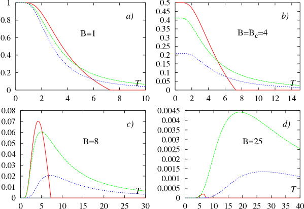
Figure 4: (Color online) (a) E (solid line), Qd (long-dashed line) and CC (short-dashed line) vs T plots for the thermal state of two qubits in the Heisenberg model at the magnetic field $B=1$ ($B<B_{c}$). (b) Identical plot for $B=B_{c}=4$. (c) Identical plot for $B=8$ ($B>B_{c}$). (d) Plot of the previous quantities for a high value of $B$ ($B=25$). See text for details.

References

- (1) Werner R F 1989 Phys. Rev. A 40 4277
- (2) Ollivier H and Zurek W H 2001 Phys. Rev. Lett. 88 017901
- (3) Nielsen M A and Chuang I L 2002 Quantum Computation and Quantum Information (New York: Cambridge University Press)
- (4) Brukner C, Zukowski M and Zeilinger A 2002 Phys. Rev. Lett. 89 197901
- (5) Barrett J, Hardy L and Kent A 2005 Phys. Rev. Lett. 95 010503; Acín A, Gisin N and Masanes Ll 2006 Phys. Rev. Lett. 97 120405; Acín A et al 2007 Phys. Rev. Lett. 98 230501
- (6) Dakic B, Vedral V and Brukner C 2010 Phys. Rev. Lett. 105 190502
- (7) Ferraro A, Aolita L, Cavalcanti D, Cucchietti F M and Acín A 2010 Phys. Rev. A 81 052318
- (8) Datta S 2008 Phys. Rev. Lett. 100 050502
- (9) Lu S and Fu S 2010 Phys. Rev. A 82 034302
- (10) Datta S arXiv [quant-ph] 1003.5256.
- (11) Lieb E, Schultz T and Mattis D 1961 Ann. of Phys. 16 407
- (12) Chandler D 1987 Introduction to Modern Statistical Mechanics (New York: Oxford University Press); Mermin N D and Wagner H 1966 Phys. Rev. Lett. 17 1133; Olsson P 1995 Phys. Rev. B 52 4526; Teitel S and Jayaprakash C 1983 Phys. Rev. B 27 598
- (13) Barouch E, McCoy B and Dresden M 1970 Phys. Rev. A 2 1075; Barouch E and McCoy B 1971 Phys. Rev. A 3 786
- (14) Recall that a QPT is a qualitative change that occurs in the ground state of a many-body system due to modifications either in the interactions among its constituents or due to the effect of an external probe.
- (15) Sachdev S 1999 Quantum Phase Transitions (Cambridge: Cambridge University Press)
- (16) Baroni F, Fubini A, Tognetti V and Verrucchi P 2007 J. Phys. A: Math. Theor. 40 9845
- (17) Galve F, Giorgi G L and Zambrini R 2011 Phys. Rev. A 83 012102
- (18) Batle J et al (2011) arXiv:quant-ph/1103.0704
- (19) Batle J and Casas M 2010 Phys. Rev. A 82 062101
- (20) Batle J and Casas M, e-print arXiv:quant-ph/1102.4653, and references therein
- (21) Werlang T et al 2010 Phys. Rev. Lett. 105 095702
- (22) Baxter R J 1982 Exactly solved models in statistical mechanics (London: Academic Press)
- (23) Arnesen M C, Bose S and Vedral V 2001 Phys. Rev. Lett. 87 017901
- (24) Gisin N 1991 Phys. Lett. A 154 201
- (25) Batle J and Casas M (in preparation)
- (26) Sen(De) A et al (2004) Phys. Rev. A 70 060304; Batle J 2006 PhD thesis quant-ph/0603124v1
- (27) Osterloh A et al 2002 Nature 416 608