Canny Algorithm: A New Estimator for Primordial Non-Gaussianities

Abstract

We utilize the Canny edge detection algorithm as an estimator for primordial non-Gaussianities. In preliminary tests on simulated sky patches with a window size of 57 degrees and multipole moments $l$ up to 1024, we find a $3\sigma$ distinction between maps with local non-Gaussianity $f_{NL}=350$ (or $f_{NL}=-700$) and Gaussian maps. We present evidence that high resolution CMB studies will strongly enhance the sensitivity of the Canny algorithm to non-Gaussianity, making it a promising technique to estimate primordial non-Gaussianity.

I Introduction

An important emerging issue in contemporary cosmology is to search for signatures of primordial non-Gaussianities in the Cosmic Microwave Background (CMB). A single field inflation scenario with standard kinetic term, slow roll potential, and standard vacuum initial condition produces a nearly scale-invariant and nearly Gaussian distribution of fluctuations in the CMB, while generalizations of the simplest model, as well as alternatives to inflation, can lead to non-Gaussianities with different sizes and shapes. Thus, a detection of non-Gaussianity would be a significant discovery, providing strong hints about the nature of inflationary or alternative models.

Among different types of non-Gaussianities, the most natural and well studied one is the local shape non-Gaussianity,

$$\Phi(x)=\Phi_{g}(x)+f_{NL}\left(\Phi_{g}(x)^{2}-\langle\Phi_{g}(x)^{2}\rangle\right)+g_{NL}\Phi_{g}^{3}(x)+\cdots\ ,$$ (1)

where $\Phi_{g}(x)$ is a field of Gaussian fluctuations. In this note, we focus on the lowest order of this local form non-Gaussianity, parameterized by $f_{NL}$.

Currently there have been a number of methods to search for non-Gaussian signatures, for example, bispectrum analysis Komatsu and Spergel (2001), Minkowski functionals Shandarin et al. (2002), and mode decomposition Fergusson and Shellard (2007). When applied to WMAP Komatsu et al. (2010) data with resolution of 0.21 degrees, current constraints of non-Gaussianity are of order $-10<f_{NL}<74$ (95% CL) from the bispectrum method. Current CMB experiments such as Planck Tauber et al. (2010) with resolution of 5 arcminutes, the Atacama Cosmology Telescope Kosowsky (2003) with resolution of 0.9 arcminutes, and the South Pole Telescope Ruhl et al. (2004) with resolution of 0.25 arcminutes will result in improved constraints with their expanded range of multipole moments and increased sensitivity and resolution.

We will explore whether edge detection algorithms are efficient at distinguishing non-Gaussian from Gaussian CMB skies. In recent years, there has emerged an interest in applying the Canny algorithm Canny (1986), an edge detection algorithm which searches for steep gradients in images, to cosmological data Amsel et al. (2008); Stewart and Brandenberger (2009); Danos and Brandenberger (2010a, b); Feeney et al. (2010). When applied to CMB temperature maps, the Canny algorithm selects the steep gradients in temperature and stores them as edges. For example, an edge map of a temperature map in which the background possesses one temperature and the area inside a circle possesses a different temperature would appear as just the outline of the circle, since the edge of the circle is a region with a steep gradient.

Since the temperature fluctuations of Gaussian and non-Gaussian maps have different probability distributions, locally maximal gradients occur at different locations in the maps. More concretely, Pogosyan et al. (2009, 2011) have shown that the gradients of Gaussian and non-Gaussian maps have different probability distributions; as edges are a subset of gradients, we expect that the edge distribution will differ between Gaussian and non-Gaussian maps. Heuristically, Pogosyan et al. (2009, 2011) also demonstrated that the number of local temperature maxima increases (or decreases) in a non-Gaussian map as compared to a Gaussian map, along with a corresponding decrease (or increase) in the number of local minima. Since one place edges will appear is along the steep gradient between a local maximum and a local minimum, we have another reason to expect a difference in edge statistics between Gaussian and non-Gaussian maps. In this paper, we take an empirical approach to ask how sensitive the Canny algorithm is to local-form non-Gaussianity. To study this question, we have used the publicly available full sky maps provided by Elsner and Wandelt Elsner and Wandelt (2009).

In this letter, we report preliminary results testing the sensitivity of the Canny algorithm to non-Gaussianities of the local shape in the CMB. We begin with a brief discussion of our simulated skies, then review the Canny algorithm and our rough optimization of it, continue with a discussion of our statistics and results, and conclude with predictions related to current experiments and future simulations.

II Simulations

A challenge in developing new methods for detecting CMB non-Gaussianity is the production of simulated non-Gaussian CMB sky maps evolved to the time of recombination with the appropriate transfer function; this is a computationally intensive process. Fortunately, the authors of Elsner and Wandelt (2009) have provided the spherical harmonic coefficients $a_{lm}$ for a thousand realizations of full sky maps for both the linear and nonlinear components of the CMB with a local form of non-Gaussianity. That is, they provide the set of $a_{lm}$ for both the $\Phi_{g}$ and $\Phi_{g}^{2}$ terms in (1). These simulations include up to mulitpole moments of $l=1024$; the spectrum of $C_{l}$ used in the simulations is available with their simulations. With these simulated maps, the work of constructing local shape non-Gaussian maps reduces to a superposition between the Gaussian and the non-Gaussian maps, with coefficient $f_{NL}$ in front of the non-Gaussian maps. We anticipate future studies when simulations with higher multipole moments and non-trivial trispectra are available.

Since our current implementation of the Canny algorithm requires the flat sky approximation, we cut approximately 57 degree by 57 degree Cartesian windows from these simulations. These window sizes are compatible with the flat sky approximation. Any distortion due to the Cartesian slicing and flat sky approximation applies equally to both the Gaussian and non-Gaussian maps and hence does not affect our results.

As a check that our algorithm is not sensitive to differences between independent Gaussian maps, we have compared two sets of 120 Gaussian maps using the statistics described below. We find that there is a 96% chance that two sets of maps drawn from the same distribution would have greater statistical differences, so they are indistinguishable. In addition, we have checked that the non-Gaussian maps and Gaussian maps have the same spectrum ($C_{l}$).

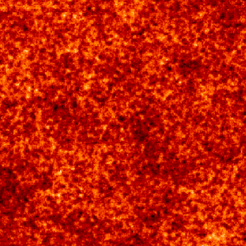
Figure 1: A sample of the Gaussian map, in a window of 57 degree by 57 degree sky.

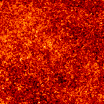
Figure 2: A sample of the non-Gaussian map with $f_{NL}=1000$, in a window of 57 degree by 57 degree sky.

III Review of Canny Algorithm

We refer the reader to Danos and Brandenberger (2010a) for a complete description of our implementation of the Canny algorithm. In brief, we search for local maxima in the gradient of the map along the direction of the gradient, in the following steps:

1. Convert the temperature map to a gradient map, recording magnitude and direction of the derivative at each pixel.

2. Scan the map along eight directions (vertically, horizontally, and along both diagonals) retaining only local maxima along the direction of the gradient.

3. Filter the remaining gradient map such that only gradients with magnitudes between a lower threshold $t_{l}$ and a cut-off threshold $t_{c}$ are kept.

4. Impose an upper threshold $t_{u}$. The remaining points above this threshold are considered as belonging to an edge. Points below this threshold are considered as belonging to an edge only if they are connected to an edge in a direction perpendicular to their gradient.

5. Count and store the numbers and lengths of edges to perform statistical analysis.

The thresholds are measured in units of a maximal gradient $G_{m}$, which we define as the lesser of the averages of the maximum gradient magnitude for all the Gaussian and non-Gaussian maps. Again, we refer the reader to Danos and Brandenberger (2010a) for more details.

One significant change made for the above standard implementation refers to Appendix A of Danos and Brandenberger (2010a), which removes doubles of locally maximal gradients. In choosing which doubled pixel to discard, instead of choosing the pixel with lower temperature, which artificially introduces more edges with lower temperature fluctuations, we chose the pixel with the lower absolute value of the temperature fluctuation.

In addition, we implemented a routine to optimize the thresholds used. We sampled ten values of the threshold parameters and minimized the quadratic fit to the probabilities for $f_{NL}=1000$ (see the description of our statistics below). The final thresholds used were $t_{c}=3.09414$, $t_{u}=0.257424$, and $t_{l}=0.104205$.

IV Statistics and Results

To differentiate statistically between sets of Gaussian and non-Gaussian simulated images, we applied the same tests as described in Danos and Brandenberger (2010a) for detection of cosmic strings. In brief, for each CMB map (a window of 500 pixels on a side), we divided all the edges into bins by edge length; all edges longer than a determined maximum length $k$ were binned with that length. Then we found the distribution of all the windows within each bin for both Gaussian and non-Gaussian maps. At that point, we apply the Student t-test to the two distributions in each bin. From the t-test we obtained the $p$-values, which give probability information, which we then combined using the Fisher combined probability test,

$$\chi_{2k}^{2}=-2\sum_{l=1}^{k}\ln(p_{l})\ ,$$ (2)

to compute the total $\chi^{2}$ separating the two sets of maps, which follows the $\chi^{2}$ distribution with $2k$ degrees of freedom. We then find the probability that the two sets of CMB maps could have that value of $\chi^{2}$ (or larger) if they were drawn from the same larger distribution of maps. In the following, we use an optimal value of $k=2$.

We applied the Canny algorithm and statistical analyses to 120 windows of approximately 57 degrees (500 pixels) per side and an $f_{NL}=350$. Our results indicate that there is a 0.1% probability that the non-Gaussian simulations and Gaussian simulations would have such a large value of $\chi^{2}$ if drawn from the same distribution, which would constitute a $3\sigma$ detection. We find similar statistical significance distinguishing Gaussian simulations and simulations with a negative non-Gaussianity parameter of $f_{NL}=-700$. The statistics for the comparison of $f_{NL}=350$ and Gaussian simulations are plotted in figure 3, showing the distribution in each bin. As a comparison, statistics for $f_{NL}=1000$ are also shown in figure 4. An astute reader will note that the Gaussian simulations give different edge counts in the two figures; this is because they are compared to simulations with different amounts of non-Gaussianity, resulting in different values of the parameter $G_{m}$ defined above.

The reader will also note that our $3\sigma$ detection level is asymmetric in $f_{NL}$; that is, it seems possible to distinguish smaller $|f_{NL}|$ from Gaussian maps if the sign of $f_{NL}$ is positive. We have checked that this is not due to a bias in the algorithm by reversing the sign of all temperature fluctuations on a set of maps; these maps give edge counts that are indistinguishable from the original set of maps. It appears that the asymmetry is an intrinsic property of local-type non-Gaussianity due to the nonlinearity of the fluctuations.

As the Canny algorithm is designed to detect edges, it may be possible to optimize it for the study of primodial non-Gaussianity (for example, by finding new statistics to differentiate Gaussian and non-Gaussian skies). However, there are also prospects for improvement even with the un-modified algorithm and statistics presented here. For example, our method is sensitive to the number of pixels in each window. A comparison of the same non-Gaussian and Gaussian simulations in windows with 200 pixels per side yields a probability of 16.3%. Therefore, we expect that the better resolutions offered by future simulations and experiments such as Planck, ACT, and SPT should allow greater sensitivity.

In contrast, our results were less sensitive to the number of windows considered. When we applied the Canny algorithm to 30 non-Gaussian realizations with $f_{NL}=350$ and 120 Gaussian realizations (we have no upper constraints to the number of Gaussian realizations we can produce), we obtained probabilities of 4% that the maps were drawn from the same distribution. In addition, we found that reducing the number of Gaussian simulations (to 30 Gaussian and 30 non-Gaussian simulations) resulted in probabilities of 17% for $f_{NL}=350$. Therefore, we conversely expect that increasing the number of Gaussian simulations could improve our results (concominant with improved resolution) due to the fact that the standard error of the mean decreases with increasing sample size. This offers another potential avenue to improve the Canny algorithm’s sensitivity to local-type non-Gaussianity.

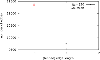
Figure 3: Edge statistics for $f_{NL}=350$. The blue (upper) dot represents the non-Gaussian simulations, and the red (lower) dot represents the Gaussian simulations. Error bars are the standard error of the mean (1$\sigma$).

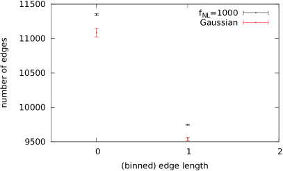
Figure 4: Edge statistics for $f_{NL}=1000$. The blue (upper) dot represents the non-Gaussian simulations, and the red (lower) dot represents the Gaussian simulations. Error bars are the standard error of the mean (1$\sigma$).

V Conclusion

We have shown that applying the Canny algorithm to segments of full sky Gaussian and non-Gaussian maps can differentiate the two sets of maps at the $3\sigma$ level down to $f_{NL}=350$ or $f_{NL}=-700$ (note that current observational limits are quoted at the 95% confidence level). Since tests of our application greatly improved for 500 pixels per window side compared to 200 pixels per window side, we anticipate that implementation of this algorithm on high resolution data should dramatically improve our results. For example, SPT Ruhl et al. (2004) will provide data with up to 2400 pixels per 10 degree side. In particular, our tests indicated that larger pixel numbers were more relevant to substantially improved results than larger numbers of images. For this reason, application of the Canny algorithm to Planck Tauber et al. (2010), ACT Kosowsky (2003), and SPT Ruhl et al. (2004) data should also be very promising for detection of primordial non-Gaussianities.

In the present note, we considered the local type bispectrum as the form of non-Gaussianity of interest. However, our method is general and can be performed on non-Gaussian maps with other types of non-Gaussianity, namely bispectra with other shapes as well as a nontrivial trispectrum. We especially expect our estimator to be sensitive to the local shape trispectrum, where the Gaussian distribution is deformed by kurtosis instead of skewness. In this case the slope of the probability distribution function is changed symmetrically, so more (less) edges should be produced when the kurtosis is positive (negative) respectively.

On the other hand, it remains unclear whether we can distinguish different types or shapes of non-Gaussianity or the contribution from cosmic strings. We will leave the comparison between these signals to future work.

In our current approach, the error bars in the figures are determined numerically by simulations of Gaussian and non-Gaussian maps. It remains interesting to see whether these error bars could also be determined theoretically. In Pogosyan et al. (2011), the extrema counts for CMB maps are calculated theoretically. It may be possible to obtain analytical bounds on edge number statistics. The analytical extrema counts may also suggest new types of statistical analysis to perform on edge maps.

Another important issue that we have not addressed in the present note is to add noise to the simulated maps. By adding noise, according to the sensitivities of WMAP, Planck, SPT or ACT, we could tell what value of $f_{NL}$ could be detected in the corresponding experiments using the Canny algorithm. We hope to address this issue in the future.

Finally, the Canny algorithm is originally developed to detect edges instead of non-Gaussianity. Thus, although we have shown that the algorithm is sensitive to non-Gaussianity, we expect there is considerable potential to optimize the algorithm, such as through the identification of a new statistic to distinguish Gaussian and non-Gaussian maps. Therefore, we are optimistic about the potential of the Canny algorithm for development as an estimator of non-Gaussianity in the CMB.