Holographic Matter : Deconfined String at Criticality

Abstract

We derive a holographic dual for a gauged matrix model in general dimensions from a first-principle construction. The dual theory is shown to be a closed string field theory which includes a compact two-form gauge field coupled with closed strings in one higher dimensional space. Possible phases of the matrix model are discussed in the holographic description. Besides the confinement phase and the IR free deconfinement phase, there can be two different classes of critical states. The first class describes holographic critical states where strings are deconfined in the bulk. The second class describes non-holographic critical states where strings are confined due to proliferation of topological defects for the two-form gauge field. This implies that the critical states of the matrix model which admit holographic descriptions with deconfined string in the bulk form novel universality classes with non-trivial quantum orders which make the holographic critical states qualitatively distinct from the non-holographic critical states. The signatures of the non-trivial quantum orders in the holographic states are discussed. Finally, we discuss a possibility that open strings emerge as fractionalized excitations of closed strings along with an emergent one-form gauge field in the bulk.

I Introduction

Extracting dynamical information on strongly interacting critical states of matter is in general a hard problem in theoretical physics. Fortunately, there are classes of strongly coupled quantum field theories whose non-perturbative dynamics can be accessed through dual descriptions which become weakly coupled when the number of degrees of freedom is large.

One such dual description that has been extensively studied in condensed matter physics is the so-called slave-particle formulationANDERSON ; BASKARAN ; SL_REVIEW . In this theory, a gauge redundancy is introduced in order to take into account dynamical constraints imposed by strong interactions. Unphysical states introduced in the redundant description is projected out by a dynamical gauge field. In the large $N$ limit, where $N$ is the number of flavor degrees of freedom, the dynamical gauge field becomes weakly coupled and emerges as a low energy collective excitation of the system.

The slave-particle theory may be viewed as a mere change of variables which allows one to compute dynamical properties conveniently, which could have been computed using a different set of variables albeit more complicated. However, the real power of the mathematical reformulation lies in the fact that it allows one to classify various novel phases of matter beyond the symmetry breaking schemeWen_SL . In particular, those phases that support emergent gauge boson possess subtle quantum orders that make them qualitatively distinct from the conventional phases. Because of the non-trivial quantum orders, the phases with an emergent (deconfined) gauge boson can not be smoothly connected to the conventional phases. Signatures of the non-trivial quantum order include fractionalized excitations and protected gapless excitations (or ground state degeneracy on a space with a non-trivial topology).

The gauge-string correspondence is another type of dualityMALDACENA ; GUBSER ; WITTEN . According to the duality, a class of $D$-dimensional quantum field theories is dual to a $(D+1)$-dimensional string theory. The question we would like to address in this paper is : Do those phases that admit holographic descriptions in one higher dimensional space possess non-trivial quantum orders ? If so, what we call holographic states that can be described in one higher dimensional space can not be smoothly connected to the conventional non-holographic states. We claim that the answer to this question is ‘yes’. The signatures of the non-trivial quantum order in holographic phases are the emergent space with an extra dimension, deconfined strings and the existence of an operator whose scaling dimension is protected from acquiring a large quantum correction at strong coupling in the large $N$ limit, even though the operator is not protected by any microscopic symmetry of the model.

The paper is organized in the following way. In Sec. II, we start by reviewing the slave-particle theory with an emphasis on quantum order in fractionalized phases. In Sec. III, we introduce a gauged matrix model which will be the focus of the rest of the paper. The model is general enough to include the $U(N)$ gauge theory. In Sec. IV, through a first-principle derivation, we show that the matrix model in general dimensions is holographically dual to a closed string field theory in one-higher dimensional spaces. In Sec. V, it is shown that the partition function of the original matrix model can be interpreted as a transition amplitude between quantum many-loop states in the holographic description. In Sec. VI, we show that the holographic description has a gauge redundancy, and strings are coupled with a compact two-form gauge field in the bulk. Because of the compact nature of the two-form gauge field, topological defects for the two-form gauge field are allowed. In Sec. VII, we discuss possible states of the matrix model. Different states are characterized by different dynamics of topological defects in the bulk. If topological defects are gapped, strings are deconfined in the bulk, and the holographic state is stable. On the other hand, if topological defects are condensed, strings are confined, and the bulk description is not useful anymore. Suppressed topological defect in the holographic phase is responsible for a non-trivial quantum order which protects the scaling dimension of the phase mode of Wilson loop operators from acquiring a large quantum correction at strong coupling in the large $N$ limit. We discuss the differences between the holographic and non-holographic states. The holographic critical phases can be divided further into two different classes. In the first case, there exist only closed strings in the bulk. In the second case, there are both closed and open strings, where open strings emerge as fractionalized collective excitations of closed strings. The latter state has a yet another quantum order which supports an emergent one-form gauge field in the bulk. Finally, we close with speculative discussions on a possible phase diagram, a world sheet description of deconfined strings, and a continuum limit.

The present construction is beyond the level of identifying the equations of motion in the bulk with the beta function of the boundary theory. We construct a full quantum theory of string in the bulk that is dual to the boundary theory. The construction of the dual theory makes use of the fact that loop variables associated with Wilson loops become classical objects in the planar limit of matrix modelsPOLYAKOV80 ; SAKITA ; MM ; JEVICKI81 . The current construction of the string field theory is directly based on the earlier worksSLEE10 ; SLEE11 . Compared to the the previous work on the $U(N)$ gauge theorySLEE11 , the present construction has two major improvements. First, the extra dimension generated out of the renormalization group flow is continuous, while the earlier construction produces a discrete extra dimension. The infinitesimally small parameter associated with a continuously increasing length scale allows one to write the bulk action in a compact form in this formalism. As a result, one can readily take a continuum limit starting from a boundary theory defined on a lattice. Second, the earlier construction involves infinitely many loop fields in the bulk associated with multi-trace operators, which makes the theory highly redundant. In the present construction, the relation between single-trace operators and multi-trace operators are explicitly implemented. As a result, the dual theory can be written only in terms of the loop fields for single-trace operators. Because of these improvements, the dual theory takes a much simpler form, and this transparency allows one to uncover deeper structures in the theory.

There also exist alternative approaches to derive holographic duals for general quantum field theoriesEMIL ; DAS ; Gopakumar:2004qb ; KOCH ; POLCHINSKI09 ; Douglas:2010rc ; SUNDRUM . All these constructions including the present one are based on the notion that the extra dimension in the holographic description is related to the length scale in the renormalization group flowVERLINDE ; LI ; HEEMSKERK10 ; Faulkner1010 ; SIN2011 .

II Quantum order in fractionalized phase

In this section we review some of the key features of the slave-particle theoryANDERSON ; BASKARAN ; SL_REVIEW using a pedagogical model introduced in Ref. GAUGE . We consider a model defined on the four-dimensional Euclidean hypercubic lattice,

$$\displaystyle S = -t\sum_{<i,j>}\sum_{a,b}\cos\left(\theta^{ab}_{i}-\theta^{ab}_{j}\right)$$ (1)

$$-K\sum_{i}\sum_{a,b,c}\cos\left(\theta^{ab}_{i}+\theta^{bc}_{i}+\theta^{ca}_{i}\right).$$

Here $\theta_{i}^{ab}$’s describe phase fluctuations of boson fields defined at site $i$. Each boson carries one flavor index $a$ and one anti-flavor index $b$ with $a,b=1,2,...,N$. $<i,j>$ represents nearest neighbor bonds of the lattice. We assume that the phases satisfy the constraints $\theta^{ab}=-\theta^{ba}$. With the constraints, there are $N(N-1)/2$ independent boson fields per site. The theory has $U(1)^{N-1}$ global symmetry under which the boson fields transform as $\theta^{ab}_{i}\rightarrow\theta^{ab}_{i}+\varphi^{a}-\varphi^{b}$.

In the weak coupling limit ($K<<1$), the model describes weakly coupled bosons. As the strength of the kinetic term $t$ is increased, there is a phase transition from the disordered phase to the bose condensed phase. In the disordered phase, all excitations are gapped. In the condensed phase, there are $(N-1)$ Goldstone modes. (At the special point of $K=0$, there are $N(N-1)/2$ Goldstone modes due to the enhanced symmetry).

In the strong coupling limit ($K>>1$), the large potential energy imposes an additional set of dynamical constraints, $\theta^{ab}_{i}+\theta^{bc}_{i}+\theta^{ca}_{i}=0$ which is solved by a decomposition,

$$\displaystyle\theta^{ab}_{i}=\phi^{a}_{i}-\phi^{b}_{i}.$$ (2)

Here $\phi_{i}^{a}$’s are boson fields which parameterize the low energy manifold. Note that these fields carry only one flavor quantum number contrary to the original boson fields. The new bosons are called slave-particles (or partons). The low energy effective action for the slave-particles becomes

$$\displaystyle S = -t\sum_{<i,j>}\left[\sum_{a}e^{i(\phi^{a}_{i}-\phi^{a}_{j})}\right]\left[\sum_{b}e^{-i(\phi^{b}_{i}-\phi^{b}_{j})}\right].$$ (3)

Note that this theory has a $U(1)$ gauge symmetry,

$$\displaystyle\phi^{a}_{i}\rightarrow\phi^{a}_{i}+\varphi_{i}.$$ (4)

This is due to the $U(1)$ redundancy introduced in the decomposition in Eq. (2). Because of the gauge symmetry, the slave-particles can not hop by themselves. However, these particles can move in space by exchanging their positions with other particles. For example, in Eq. (3), the particle with flavor $a$ can hop from site $j$ to $i$ as the particle with flavor $b$ hops from $i$ to $j$. In this sense, they can move only through the help of other slave-particles. One can introduce a collective hopping field $\chi_{ij}\equiv\sum_{b}e^{-i(\phi^{b}_{i}-\phi^{b}_{j})}$ to characterize the amplitude of this mutual hopping. If we use this collective field, Eq. (3) can be written as

$$\displaystyle S = -t\sum_{<i,j>,a}\chi_{ij}e^{i(\phi^{a}_{i}-\phi^{a}_{j})}.$$ (5)

The magnitude of the collective field characterizes the strength of hopping, and the phase plays the role of the U(1) gauge field to which the slave-particles are coupled electrically. This mapping from Eq. (3) to the U(1) gauge theory can be made more rigorous, by using the Hubbard-Stratonovich transformationGAUGE . Although the gauge field does not have the usual Maxwell’s term, the kinetic energy is generated once high energy modes of the boson fields are integrated out, which renormalizes the gauge coupling from infinity to $g^{2}\sim 1/N$. It is clear that slave-particles can propagate coherently in space only when the hopping field is ‘condensed’, and provides a smooth background. Since the hopping field is not a gauge invariant quantity, we need to be careful when we say that the hopping field is condensed. This notion can be sharply characterized by examining dynamics of topological defect.

Because the U(1) gauge field is compact, monopole is allowed as a topological defect in the theory. The mass of monopole is $O(N)$ for a large $N$. Whether the slave-particles arise as low energy excitations of the theory depends on the dynamics of monopole. One can consider the following three different phases.

1. Confining phase

   For a small $N$ and small $t$, monopoles are light, and slave-particles are heavy. If monopoles are condensed, strong fluctuations of the phase mode of the hopping field confine the slave-particles. Only gauge neutral composite particles, which are nothing but the original bosons in Eq. (1), appear as low energy excitations. In this phase, all excitations are gapped. This phase is adiabatically connected to the disordered phase in the weak coupling limit.

2. Higgs phase

   This is the phase which is electromagnetically dual to the confining phase. The slave-particles are condensed when $t$ is large. As a result of the condensation of charged fields, monopoles and anti-monopoles are connected by vortex lines which produce a linearly increasing potential : monopoles and anti-monopoles are confined. One slave-particle is eaten by the massive U(1) gauge boson, and $(N-1)$ gapless bosons are left. These modes are the Goldstone modes. This phase is smoothly connected to the bose condensed phase in the weak coupling limit.

3. Fractionalized (Coulomb) phase

   For a large $N$, the mass of monopole is large. When both the slave-particles and monopoles are gapped, the Coulomb phase is realized. In this phase, slave-particles are deconfined, and arise as (gapped) excitations of the system. They are fractionalized modes because they carry only half the flavor quantum number of the original bosons. Moreover, the U(1) gauge field arises as a gapless excitation. It is noted that the gapless excitation in this phase is not a Goldstone mode. It is not protected by any microscopic symmetry. Saying that there is a gapless gauge boson in a gauge theory may sound trivial. However, we have to remember that the gauge boson is nothing but a collective excitation of the original boson fields. The existence of a collective excitation which remains gapless without a fine tuning is actually something remarkable : someone who does not use the language of gauge theory would find the origin of the gapless collective excitation mysterious. It turns out that the gapless mode is protected by a subtle order which is not characterized by any symmetry breaking scheme. This order, dubbed as quantum orderWen_SL , is associated with suppression of topological excitation, monopole in the long distance limit. Formally, this order can be expressed as the emergence of the Bianchi identity $dF=0$ in the long distance limit, where $F$ is the field strength for the emergent gauge field. The key features of the non-trivial quantum order is the presence of the fractionalized excitations and the emergent gauge field. Note that slave-particles are not gauge invariant objects. However, $\phi^{a}$’s become ‘classical’ in the large $N$ limit where non-perturbative fluctuations of the hopping field are suppressed. In this regard, fractionalization is associated with the emergence of an ‘internal’ space.

Table 1:

	slave-particle	monopole	low energy excitations
Confining phase	confined	condensed	$\theta^{ab}$
Coulomb phase	deconfined	gapped	$\phi^{a}$, monopole, gauge boson
Higgs phase	condensed	confined	Goldstone bosons

Table. I summarizes the physics in each phase of the boson model. Now, we switch gear to discuss about a matrix model and its possible phases. We will draw a close analogy between the quantum order present in the Coulomb phase of the boson model and a quantum order present in the holographic phase of the matrix model. We will see that the holographic phase has a distinct quantum order associated with the emergence of an ‘external’ space.

III Matrix model

We start with a matrix model defined on the D-dimensional Euclidean hypercubic lattice,

$$\displaystyle Z=\int dU~{}~{}e^{-S[U]}$$ (6)

with the action,

$$\displaystyle S[U]=NM^{2}\sum_{<i,j>}\mbox{tr}(U_{ij}^{\dagger}U_{ij})+N^{2}V\left[\frac{1}{N}W_{C}\right].$$ (7)

Here $i$, $j$ are site indices in the lattice with lattice spacing $a$, and $U_{ij}=U_{ji}^{\dagger}$ is $N\times N$ complex matrix defined on the nearest neighbor bond $<i,j>$. $W_{C}$ is Wilson line defined on the closed oriented loop $C$,

$$\displaystyle W_{C} = \mbox{tr}\left[\prod_{<ij>\in C}U_{ij}\right],$$ (8)

where the product is ordered along the path. $V[W_{C}/N]$ is a function of Wilson loop operators,

$$\displaystyle V = -\sum_{n=1}^{\infty}N^{-n}\sum_{\{C_{1},..,C_{n}\}}J_{\{C_{1},..,C_{n}\}}\prod_{k=1}^{n}W_{C_{k}}$$ (9)

which is, in general, non-linear in the presence of multi-trace operators. Here $J_{\{C_{1},..,C_{n}\}}$’s are loop dependent coupling constants. This theory is invariant under the $U(N)$ gauge transformation : $U_{ij}\rightarrow V_{i}^{\dagger}U_{ij}V_{j}$. Eq. (6) may be viewed as the partition function for a $(D-1)$-dimensional quantum matrix model in the imaginary time formalism.

To see that this model includes the usual $U(N)$ gauge theory, we consider the following quartic action in Eq. (7) as an example,

$$\displaystyle N^{2}V = \sum_{<i,j>}\left[-NM_{0}^{2}~{}\mbox{tr}(U_{ij}^{\dagger}U_{ij})+Nv~{}\mbox{tr}(U_{ij}^{\dagger}U_{ij}U_{ij}^{\dagger}U_{ij})+v^{{}^{\prime}}~{}\left\{\mbox{tr}(U_{ij}^{\dagger}U_{ij})\right\}^{2}\right]$$ (10)

$$-NJ~{}\sum_{\Box}W_{\Box},$$

where $\Box$ represents unit plaquettes on the lattice. Here $M_{0}^{2}>0$, $v>0$, $v^{{}^{\prime}}>0$. We assume that $v^{{}^{\prime}}$ is sufficiently large compared to $J$. The relative magnitude of $M$ and $M_{0}$ determines the shape of the potential for the matrix field. For small $M_{0}$, $U_{ij}=0$ is the minimum, and the system is fully gapped. For large $M_{0}$, the low energy manifold is spanned by the matrices that satisfy $U_{ij}U_{ij}^{\dagger}=uI$ with $u\sim\frac{M_{0}^{2}-M^{2}}{2(v+v^{{}^{\prime}})}$. In this case, the low energy effective theory becomes the $U(N)$ lattice gauge theory with the ’t Hooft coupling $\lambda\sim(Ju^{4})^{-1}$. This theory can be viewed as a ‘linear sigma model’ for the $U(N)$ gauge theory. Presumably, the gapped phase in the small $M_{0}$ limit is smoothly connected to the confinement phase of the gauge theory. As $M_{0}$ is increased further, the system can go through a phase transition to the deconfinement phase at a critical coupling $M_{0}^{c}$, depending on the dimension. If the phase transition is continuous, we can take the continuum limit by taking $a\rightarrow 0$ and $M_{0}\rightarrow M_{0}^{c}$ such that the confining scale is fixed.

IV General Construction

In this section, we construct a holographic dual for the matrix model in Eq. (7) with general potential $V$ in general dimensions. We will follow the idea introduced in Ref. SLEE10 where coupling constants are lifted to dynamical fields in the bulk space where the extra dimension corresponds to the length scale of the renormalization group flow. In the presence of multi-trace operators, this formalism becomes rather complicatedSLEE11 because one has to introduce independent fields for infinitely many multi-trace operators that are generated along the renormalization group flow. This issue is present even though multi-trace operators are not turned on initially, because they are generated at low energy scales in any case. To avoid this complication, here we express multi-trace operators in terms of single-trace one, by introducing a complex auxiliary field $\phi_{C}$ for each loop $C$ (see Appendix A),

$$\displaystyle Z=\int dUd\phi_{C}^{(0)}d\phi_{C}^{(0)*}~{}~{}e^{-S_{1}},$$ (11)

where

$$\displaystyle S_{1} = NM^{2}\mbox{tr}(U_{ij}^{\dagger}U_{ij})+N^{2}\phi_{C}^{(0)}(\phi_{C}^{(0)*}-W_{C}/N)+N^{2}V[\phi_{C}^{(0)*}].$$ (12)

Here we dropped a multiplicative numerical factor in the partition function, which is not important. It is noted that $Z$ is well defined although $S_{1}$ is not bounded from below as a function of $\phi_{C}^{(0)}$ and $\phi_{C}^{(0)*}$. This is because $S_{1}$ is complex and contributions from large negative $S_{1}$ is canceled because of rapid oscillation in phase. The repeated indices $ij$ and $C$ are understood to be summed over nearest neighbor links and closed loops, respectively.

To perform a real space renormalization groupPOLCHINSKI84 ; POLONYI ; SLEE10 , an auxiliary matrix field $\tilde{U}_{ij}$ is introduced in each link,

$$\displaystyle Z=(N^{1/2}\mu)^{N^{2}{\cal N}_{l}}\int d\phi_{C}^{(0)}d\phi_{C}^{(0)*}dUd\tilde{U}~{}~{}e^{-S_{2}},$$ (13)

where

$$\displaystyle S_{2} = S_{UV}[\phi_{C}^{(0)*},\phi_{C}^{(0)}]-N\phi_{C}^{(0)}W_{C}$$ (14)

$$+NM^{2}\mbox{tr}(U_{ij}^{\dagger}U_{ij})+N\mu^{2}\mbox{tr}(\tilde{U}_{ij}^{\dagger}\tilde{U}_{ij}).$$

Here ${\cal N}_{l}$ is the number of links in the lattice, and

$$\displaystyle S_{UV}[\phi_{C}^{(0)*},\phi_{C}^{(0)}] = N^{2}\Bigl{\{}\phi_{C}^{(0)}\phi_{C}^{(0)*}+V[\phi_{C}^{(0)*}]\Bigr{\}}$$ (15)

is an action for $\phi_{C}^{(0)}$. We change the variables as

$$\displaystyle U_{ij} = e^{-\alpha dz}(u_{ij}+\tilde{u}_{ij}),$$

$$\tilde{U}_{ij} = e^{-\alpha dz}(Au_{ij}+B\tilde{u}_{ij}),$$ (16)

where $\alpha$ is a positive constant, $dz$ is an infinitesimally small parameter, and

$$A=-\frac{M^{2}}{m\mu},~{}~{}B=\frac{m}{\mu},$$ (17)

with

$$\displaystyle m^{2} = \frac{M^{2}}{e^{2\alpha dz}-1}.$$ (18)

In terms of the new variables, the partition function becomes

$$\displaystyle Z=(N^{1/2}m)^{N^{2}{\cal N}_{l}}\int d\phi_{C}^{(0)}d\phi_{C}^{(0)*}dud\tilde{u}~{}~{}e^{-S_{3}},$$ (19)

where

$$\displaystyle S_{3} = S_{UV}[\phi_{C}^{(0)*},\phi_{C}^{(0)}]-N\phi_{C}^{(0)^{\prime}}W_{C}^{{}^{\prime}}$$ (20)

$$+N\left[M^{2}\mbox{tr}(u_{ij}^{\dagger}u_{ij})+m^{2}\mbox{tr}(\tilde{u}_{ij}^{\dagger}\tilde{u}_{ij})\right].$$

Here $W^{{}^{\prime}}_{C}=\mbox{tr}\left[\prod_{<ij>\in C}(u_{ij}+\tilde{u}_{ij})\right]$, and $\phi_{C}^{(0)^{\prime}}=e^{-\alpha dzL_{C}}\phi_{C}^{(0)}$, where $L_{C}$ is the length of the loop $C$. The field $\tilde{u}_{ij}$ with the large mass $m$ has taken away a small amount of quantum fluctuations from the original field $U_{ij}$, which leaves an action for $u_{ij}$ with smaller couplings $\phi_{C}^{(0)^{\prime}}$. Therefore, we can interpret $u_{ij}$’s as low energy fields and $\tilde{u}_{ij}$’s as high energy fields.

Figure 1: A loop with a self-retracting link splits into two loops (a), becomes shorter (b), or disappears (c), as the matrix field $\tilde{u}_{ij}$ on the link is integrated out. In (d), two loops which share a link merge into one.

Fluctuations of $\tilde{u}_{ij}$ renormalize the (dynamical) couplings for the low energy field $u_{ij}$. Integrating over $\tilde{u}_{ij}$, we obtain

$$\displaystyle Z=\int d\phi_{C}^{(0)}d\phi_{C}^{(0)*}du~{}~{}e^{-S_{4}}$$ (21)

to the linear order in $dz$, where

$$\displaystyle S_{4} = S_{UV}[\phi_{C}^{(0)*},\phi_{C}^{(0)}]-N\phi_{C}^{(0)^{\prime}}w_{C}$$ (22)

$$-\frac{1}{2m^{2}}F_{ij}[C_{1},C_{2}]\phi_{[C_{1}+C_{2}]_{ij}}^{(0)^{\prime}}w_{C_{1}}w_{C_{2}}-\frac{N}{2m^{2}}G_{ij}[C_{1},C_{2}]\phi_{C_{1}}^{(0)^{\prime}}\phi_{C_{2}}^{(0)^{\prime}}w_{(C_{1}+C_{2})_{ij}}$$

$$+NM^{2}\mbox{tr}(u_{ij}^{\dagger}u_{ij})$$

with $w_{C}=\mbox{tr}\left[\prod_{<ij>\in C}u_{ij}\right]$. In the third and the fourth terms, $ij$ runs over all nearest neighbor links, and $C_{1}$, $C_{2}$ are understood to run over all possible loops including null loops with the convention $\phi_{\emptyset_{i}}=0$, $\phi_{\emptyset_{i}}^{*}=1$ and $w_{\emptyset_{i}}=1$ for null loops, where $\emptyset_{i}$ refers to the null loop at site $i$. Here we regard null loops at different sites as different loops. By this, we can keep the combinatorics simpler. In the third term, $F_{ij}[C_{1},C_{2}]$ is a form factor that tells whether or not two loops $C_{1}$ and $C_{2}$ are ‘nearest neighbors’ : $F_{ij}[C_{1},C_{2}]=1$ if $C_{1}$ and $C_{2}$ can be merged into one loop by adding the link $ij$ and rejoining the loops, and $F_{ij}[C_{1},C_{2}]=0$ otherwise. $[C_{1},C_{2}]_{ij}$ denotes the loop that is made of $C_{1}$ and $C_{2}$ with the addition of the link $ij$. When both $C_{1}$ and $C_{2}$ are non-trivial loops, the third term describes a process where a loop splits into two loops (Fig. 1 (a)). When one of the two loops is a null loop, it describes a process where a loop becomes shorter by eliminating a self-retracting link (Fig. 1 (b)). When both are null loops, it describes a self-retracting link disappearing (Fig. 1 (c)). In the fourth term, $G_{ij}[C_{1},C_{2}]$ is a form factor that tells whether or not two loops $C_{1}$ and $C_{2}$ are sharing the link $ij$ : $G_{ij}[C_{1},C_{2}]=1$ if $C_{1}$ and $C_{2}$ can be merged into one loop by removing the shared link $ij$, and $G_{ij}[C_{1},C_{2}]=0$ otherwise. $(C_{1},C_{2})_{ij}$ denotes the loop that is made by merging $C_{1}$ and $C_{2}$ by removing the shared link $ij$. The fourth term describes a process where two loops merge into one loop (Fig. 1 (d)). In the small $dz$ limit, $1/m^{2}\sim O(dz)$, and we can replace $\phi_{C}^{(0)^{\prime}}$ with $\phi_{C}^{(0)}$ in the third and fourth terms of the action to the linear order in $dz$.

Note that double trace operators are generated for $u_{ij}$. Another set of auxiliary fields is introduced to express the double-trace operator in terms of single-trace operators as

$$\displaystyle Z=\int d\phi_{C}^{(0)}d\phi_{C}^{(0)*}d\phi_{C}^{(1)}d\phi_{C}^{(1)*}du~{}~{}e^{-S_{5}},$$ (23)

where

$$\displaystyle S_{5} = S_{UV}[\phi_{C}^{(0)*},\phi_{C}^{(0)}]$$ (24)

$$+N^{2}\phi_{C}^{(1)}(\phi_{C}^{(1)*}-w_{C}/N)$$

$$-N^{2}\phi_{C}^{(0)^{\prime}}\phi_{C}^{(1)*}-\frac{N^{2}}{2m^{2}}\left(F_{ij}[C_{1},C_{2}]\phi_{[C_{1}+C_{2}]_{ij}}^{(0)}\phi_{C_{1}}^{(1)*}\phi_{C_{2}}^{(1)*}+G_{ij}[C_{1},C_{2}]\phi_{C_{1}}^{(0)}\phi_{C_{2}}^{(0)}\phi_{(C_{1}+C_{2})_{ij}}^{(1)*}\right)$$

$$+NM^{2}\mbox{tr}(u_{ij}^{\dagger}u_{ij})$$

$$= S_{UV}[\phi_{C}^{(0)*},\phi_{C}^{(0)}]$$

$$+N^{2}\phi_{C}^{(1)*}(\phi_{C}^{(1)}-\phi_{C}^{(0)^{\prime}})$$

$$-\frac{N^{2}\alpha dz}{M^{2}}\left(F_{ij}[C_{1},C_{2}]\phi_{[C_{1}+C_{2}]_{ij}}^{(0)}\phi_{C_{1}}^{(1)*}\phi_{C_{2}}^{(1)*}+G_{ij}[C_{1},C_{2}]\phi_{C_{1}}^{(0)}\phi_{C_{2}}^{(0)}\phi_{(C_{1}+C_{2})_{ij}}^{(1)*}\right)$$

$$-N\phi^{(1)}_{C}w_{C}+NM^{2}\mbox{tr}(u_{ij}^{\dagger}u_{ij}).$$

If we repeatedly apply the steps in Eqs. (13) - (24) to the last line of Eq. (24) $R$ times, we obtain

$$\displaystyle Z=\int\prod_{l=0}^{R}\left[d\phi_{C}^{(l)}d\phi_{C}^{(l)*}\right]du~{}~{}e^{-S_{6}},$$ (25)

where

$$\displaystyle S_{6} = S_{UV}[\phi_{C}^{(0)*},\phi_{C}^{(0)}]$$ (26)

$$+N^{2}\Bigl{\{}\sum_{l=1}^{R}\Bigl{[}\phi_{C}^{(l)*}(\phi_{C}^{(l)}-\phi_{C}^{(l-1)}+\alpha L_{C}dz\phi_{C}^{(l-1)})$$

$$-\frac{\alpha dz}{M^{2}}\left(F_{ij}[C_{1},C_{2}]\phi_{[C_{1}+C_{2}]_{ij}}^{(l-1)}\phi_{C_{1}}^{(l)*}\phi_{C_{2}}^{(l)*}+G_{ij}[C_{1},C_{2}]\phi_{C_{1}}^{(l-1)}\phi_{C_{2}}^{(l-1)}\phi_{(C_{1}+C_{2})_{ij}}^{(l)*}\right)\Bigr{]}\Bigr{\}}$$

$$-N\phi^{(R)}_{C}w_{C}+NM^{2}\mbox{tr}(u_{ij}^{\dagger}u_{ij}).$$

What is the physical meaning of the auxiliary fields ? In the last line of Eq. (26), we note that $\phi_{C}^{(R)}$ acts as a source for the low energy matrix field at scale $e^{-Rdz}$. The key difference from the standard renormalization group procedure is that the source fields are dynamical fields rather than fixed constants at each scaleSLEE10 . On the other hand, the equation of motion for $\phi_{C}^{(R)}$ implies that

$$\displaystyle<\phi_{C}^{(R)*}>=\frac{1}{N}<w_{C}>.$$ (27)

Therefore, the conjugate field $\phi_{C}^{(R)*}$ describes the Wilson loop operator. As we will see below, $\phi_{C}$ and $\phi_{C}^{*}$ are conjugate fields which satisfy a non-trivial commutation relation : sources and operators are conjugate to each other.

Figure 2: Examples of the diagrams that contribute to the IR effective potential to the leading order in $1/N$. Every link should be paired with another link with the opposite orientation.

Finally, we integrate out $u$ to obtain

$$\displaystyle Z=\int\prod_{l=0}^{R}\left[d\phi_{C}^{(l)}d\phi_{C}^{(l)*}\right]~{}~{}e^{-S_{7}},$$ (28)

where

$$\displaystyle S_{7} = S_{UV}[\phi_{C}^{(0)*},\phi_{C}^{(0)}]$$ (29)

$$+N^{2}\Bigl{\{}\sum_{l=1}^{R}\Bigl{[}\phi_{C}^{(l)*}(\phi_{C}^{(l)}-\phi_{C}^{(l-1)}+\alpha L_{C}dz\phi_{C}^{(l-1)})$$

$$-\frac{\alpha dz}{M^{2}}\left(F_{ij}[C_{1},C_{2}]\phi_{[C_{1}+C_{2}]_{ij}}^{(l-1)}\phi_{C_{1}}^{(l)*}\phi_{C_{2}}^{(l)*}+G_{ij}[C_{1},C_{2}]\phi_{C_{1}}^{(l-1)}\phi_{C_{2}}^{(l-1)}\phi_{(C_{1}+C_{2})_{ij}}^{(l)*}\right)\Bigr{]}\Bigr{\}}$$

$$+S_{IR}[\phi^{(R)}_{C}].$$

Here $S_{IR}$ is the effective potential given by

$$\displaystyle S_{IR}[\phi^{(R)}_{C}] = -\ln\int du~{}~{}e^{-NM^{2}\mbox{tr}(u_{ij}^{\dagger}u_{ij})+N\phi^{(R)}_{C}w_{C}}.$$ (30)

For a future use, we define

$$\displaystyle V^{{}^{\prime}}[\phi^{(R)}_{C}] \equiv \frac{1}{N^{2}}S_{IR}[\phi^{(R)}_{C}],$$ (31)

which can be computed using the strong coupling expansion,

$$\displaystyle V^{{}^{\prime}}[\phi^{(R)}_{C}] = -\phi^{(R)}_{C_{1}}M^{-L_{C_{1}}}{\tilde{\delta}}_{C_{1},0}-\frac{1}{2}\phi^{(R)}_{C_{1}}\phi^{(R)}_{C_{2}}M^{-\sum_{i=1}^{2}L_{C_{i}}}{\tilde{\delta}}_{C_{1}+C_{2},0}$$ (32)

$$-\frac{1}{6}\phi^{(R)}_{C_{1}}\phi^{(R)}_{C_{2}}\phi^{(R)}_{C_{3}}M^{-\sum_{i=1}^{3}L_{C_{i}}}{\tilde{\delta}}_{C_{1}+C_{2}+C_{3},0}-....$$

Here the delta function is defined as

$$\displaystyle{\tilde{\delta}}_{C,0} \equiv \prod_{<i,j>}\delta_{Q_{ij}[C],0},$$ (33)

where $Q_{ij}[C]$ is the U(1) charge defined on link $ij$ associated with the flux of loop $C$SLEE11 . If the loop $C$ passes through the link $ij$ from $i$ to $j$ (from $j$ to $i$) $n$ times, $Q_{ij}[C]=n(-n)$. The first, second and third terms are from a self retracting loop (Fig.2 (a)), two loops (Fig.2 (b)) and three loops (Fig.2 (c)), respectively. Higher order terms can be obtained similarly. Now we take $dz\rightarrow 0$ and $R\rightarrow\infty$ limits with $\beta\equiv Rdz$ fixed. Then, the partition function is written as

$$\displaystyle Z=\int D\phi_{C}D\phi_{C}^{*}~{}~{}e^{-\left(S_{bulk}[\phi_{C}^{*}(z),\phi_{C}(z)]+S_{UV}[\phi_{C}^{*}(0),\phi_{C}(0)]+S_{IR}[\phi_{C}(\beta)]\right)},$$ (34)

where

$$\displaystyle S_{bulk} = N^{2}\int_{0}^{\beta}dz\Bigl{[}\phi_{C}^{*}\partial_{z}\phi_{C}+\alpha L_{C}\phi_{C}^{*}\phi_{C}$$ (35)

$$-\frac{\alpha}{M^{2}}\left(F_{ij}[C_{1},C_{2}]\phi_{C_{1}}^{*}\phi_{C_{2}}^{*}\phi_{[C_{1}+C_{2}]_{ij}}+G_{ij}[C_{1},C_{2}]\phi_{(C_{1}+C_{2})_{ij}}^{*}\phi_{C_{1}}\phi_{C_{2}}\right)\Bigr{]}.$$

Since the partition function is independent of $\beta$, we can take $\beta\rightarrow\infty$. From now on, we will interpret the scale parameter $z$ as an imaginary ‘time’. The dual description becomes a $(D+1)$-dimensional field theory of closed loop. Although the action is written in terms of continuous $z$, one should go back to the discrete version whenever there is an ambiguity, e.g., when extracting boundary conditions by taking variations with respect to boundary fields.

As is the case for matrix models, there are two important parameters that are independent with each other. The first is $\frac{1}{N^{2}}$ which controls the strength of quantum fluctuations of the loop fields : the whole action including the boundary actions scales as $N^{2}$. The second is the ’t Hooft coupling. In this theory, there is no unique ’t Hooft coupling. Instead there is a set of couplings defined in the space of loops, $J_{\{C_{1},..,C_{n}\}}$ which scales as the inverse of the ’t Hooft coupling. Since we could have scaled out $M^{2}$ by redefining $U_{ij}=U_{ij}^{{}^{\prime}}/M$ in Eq. (7), the theory depends only on the combination $J_{\{C_{1},..,C_{n}\}}M^{-\sum_{i}L_{C}}$. The small $J_{\{C_{1},..,C_{n}\}}$ limit is equivalent to the large $M$ limit, which corresponds to the strong coupling limit of the matrix model where one expects to have the confinement phase. The set of $J_{\{C_{1},..,C_{n}\}}$’s sets the magnitudes of loop fields in the bulk. We will see that background loop fields, in turn, control the size of strings which describe small fluctuations of the loop fields.

V Hamiltonian picture

V.1 Partition function as a transition amplitude between many-body loop states

The partition function can be viewed as an imaginary-time transition amplitude between many-body loop states. To see this, we will use a rescaled loop variable in this sub-section,

$$\displaystyle\Phi_{C}\equiv N\phi_{C}.$$ (36)

The bulk action in the new variable becomes

$$\displaystyle S_{bulk} = \int_{0}^{\infty}dz\Bigl{[}\Phi_{C}^{*}\partial_{z}\Phi_{C}+\alpha L_{C}\Phi_{C}^{*}\Phi_{C}$$ (37)

$$-\frac{\alpha}{NM^{2}}\left(F_{ij}[C_{1},C_{2}]\Phi_{C_{1}}^{*}\Phi_{C_{2}}^{*}\Phi_{[C_{1}+C_{2}]_{ij}}+G_{ij}[C_{1},C_{2}]\Phi_{(C_{1}+C_{2})_{ij}}^{*}\Phi_{C_{1}}\Phi_{C_{2}}\right)\Bigr{]}.$$

The action has the form for canonical bosonic fields, where $\Phi_{C}$ ($\Phi_{C}^{*}$) corresponds to the coherent field associated with the annihilation (creation) operator defined in the space of closed loops. The annihilation and creation operators $a_{C}$, $a_{C}^{\dagger}$ satisfy the standard commutation relation

$$\displaystyle\left[a_{C},a_{C^{{}^{\prime}}}^{\dagger}\right]=\delta_{C,C^{{}^{\prime}}},$$ (38)

where $\delta_{C,C^{{}^{\prime}}}$ is a Kronecker-delta function defined in the space of loops. Then the partition function can be written as an imaginary-time transition amplitude,

$$\displaystyle Z = \lim_{\beta\rightarrow\infty}<\Psi_{f}|e^{-\beta H}|\Psi_{i}>,$$ (39)

between the initial (UV) state at $z=0$,

$$\displaystyle|\Psi_{i}> = \int d\Phi_{C}^{*}d\Phi_{C}~{}~{}\Psi_{i}[\Phi_{C}^{*},\Phi_{C}]|\Phi_{C}>,$$ (40)

with

$$\displaystyle\Psi_{i}[\Phi_{C}^{*},\Phi_{C}] = e^{-\Phi_{C}^{*}\Phi_{C}-N^{2}V[\Phi_{C}^{*}/N]},$$ (41)

and the final (IR) state at $z=\infty$,

$$\displaystyle|\Psi_{f}> = \int d\Phi_{C}^{*}d\Phi_{C}~{}~{}\Psi_{f}[\Phi_{C}^{*},\Phi_{C}]|\Phi_{C}>,$$ (42)

with

$$\displaystyle\Psi_{f}[\Phi_{C}^{*},\Phi_{C}] = e^{-\Phi_{C}^{*}\Phi_{C}-N^{2}V^{{}^{\prime}}[\Phi_{C}^{*}/N]}.$$ (43)

Here $\Psi_{i}[\Phi_{C}^{*},\Phi_{C}]$ and $\Psi_{f}[\Phi_{C}^{*},\Phi_{C}]$ are the wavefunctions of loops written in the coherent state basis,

$$\displaystyle|\Phi_{C}>=e^{\Phi_{C}a_{C}^{\dagger}}|0>,$$ (44)

where $|0>$ is the vacuum in the Fock space of loops : $a_{C}|0>=0$ for all $a_{C}$. (For the derivation of Eqs. (41) and (43), see Appendix. B). The bulk Hamiltonian is given by

$$\displaystyle H = \alpha L_{C}a_{C}^{\dagger}a_{C}-\frac{\alpha}{NM^{2}}\Bigl{(}F_{ij}[C_{1},C_{2}]a_{C_{1}}^{\dagger}a_{C_{2}}^{\dagger}a_{[C_{1}+C_{2}]_{ij}}+G_{ij}[C_{1},C_{2}]a_{(C_{1}+C_{2})_{ij}}^{\dagger}a_{C_{1}}a_{C_{2}}\Bigr{)}.$$ (45)

The first term in the Hamiltonian describes a tension of closed loops. The second and the third terms are the interaction terms which describe the processes where one loop splits into two loops, and two loops merge into one loop, respectively, as is shown in Fig. 1. We use the convention $a_{\emptyset_{i}}=0$, $a^{\dagger}_{\emptyset_{i}}=1$ for null loops. Similar loop Hamiltonians that describe joining and splitting processes of loops were considered in matrix modelsISHIBASHI ; HAM .

This is an exact mapping between the $D$-dimensional matrix model ($(D-1)$-dimensional quantum matrix model) and the $(D+1)$-dimensional loop model (or $D$-dimensional quantum loop model). Several remarks are in order. First, the Hamiltonian in Eq. (45) is a many-body Hamiltonian that governs the quantum dynamics of loops along the scale $z$ which is interpreted as an imaginary time. It is noted that the Hamiltonian is not Hermitian. Due to the cubic interaction term, the Hamiltonian is unbounded from below. However, the transition amplitude in Eq. (39) is well defined because eigenvalues of the Hamiltonian are complex. Eigenvalues with a large negative real part in general come with a large imaginary part, and their contributions cancel with each other due to oscillation in phase. Second, the bulk Hamiltonian is universal, and it is independent of the details of the matrix model. All informations pertaining to the specifics of the matrix model are encoded in the initial wavefunction at $z=0$. Third, the strength of the interaction between loops is order of $1/N$, and loops are weakly interacting in the large $N$ limit. Therefore, the theory becomes classical in the large $N$ limit. Fourth, $H$ does not have any hopping term such as $a_{C_{1}}^{\dagger}a_{C_{2}}$ with different $C_{1}$ and $C_{2}$. This fact will become important for gauge symmetry, which will be discussed in Sec. V. For earlier works on string field theories formulated without quadratic action, see Ref. LYKKEN86 ; HOROWITZ86 .

The fact that the partition function is independent of $\beta$ has a remarkable consequence. By taking the derivative of Eq. (39) (for a finite $\beta$) with respect to $\beta$, we obtain

$$\displaystyle 0 = <\Psi_{f}|e^{-\beta H}H|\Psi_{i}>.$$ (46)

Since physical states are singlets of $H$, the Hamiltonian can be viewed as a generator of a ‘gauge transformation’. The gauge transformation corresponds to a reparameterization of $z$. It is based on the fact that one can choose different speed of renormalization group flows at different scales without affecting the physics. By choosing the parameter $\alpha$ to be $z$-dependent, the reparameterization symmetry can be made explicitSLEE10 . Here $\alpha(z)$ becomes the lapse function. Reparameterizations of $z$ form a subgroup of the full diffeomorphism in the $(D+1)$-dimensional space. It would be interesting to formulate the theory where the full diffeomorphism can be made explicit in the bulk. Here we proceed with the present formalism where we choose specific time slices along the $z$ direction.

V.2 Wilson loop operator

Figure 3: Loops are emitted at the UV boundary and propagate to the IR boundary. Since there is no hopping term in the Hamiltonian, loops can not move. Instead, they can join or split following the processes shown in Fig. 1. Two loops with opposite orientations can get pair-annihilated through multiple interactions.

Figure 4: (a) A process where a loop and its anti-loop get annihilated in pair through a series of interactions. (b) A self-retracting loop in the vacuum can split into a loop and an anti-loop.

The physical picture for the transition amplitude is the following. At the UV boundary ($z=0$), a condensate of loops are emitted and propagate in $z$ under the evolution governed by $H$. The amplitude of the condensate is $<\Phi_{C}>\sim O(N)$. This can be seen from the fact that the action for the unscaled loop fields $\phi_{C}$ has $N^{2}$ as an overall prefactor, which implies $<\phi_{C}>\sim O(1)$. Loops can join and split through the interactions as is illustrated in Fig. 3. A loop $C$ and its anti-loop $\bar{C}$, the loop with the opposite orientation, can get pair-annihilated through a series of interactions as is shown in Fig. 4 (a). Moreover, a self-retracting loop can become a loop and an anti-loop as is shown in Fig. 4 (b). As it will be shown in Sec. VII. A, loop fields for self-retracting loops have non-zero vacuum expectation values in the bulk. Therefore, a pair of loop and anti-loop can be created out of vacuum. This means that two loops with the opposite orientations act as particle and anti-particle in a relativistic field theory. Finally, those loops emitted at the UV boundary are absorbed at the IR boundary. In this sense, the UV boundary is a source of loops, and the IR boundary is a sink.

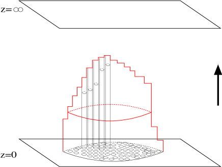
Figure 5: A world sheet formed by multiple processes where a large loop absorbs many small loops at different stages to change its shape to disappear before it reach the IR boundary.

Now let us consider a Wilson loop operator for a loop $C$ which is much larger than the size of Wilson loops for which sources are turned on at the UV boundary. The expectation value of the Wilson loop operator is given by the one-point function,

$$\displaystyle<W_{C}>=\frac{1}{N}\left.\frac{\partial\ln Z}{\partial J_{C}}\right|_{J_{C}=0}=\lim_{\beta\rightarrow\infty}\frac{<\Psi_{f}|e^{-\beta H}a_{C}^{\dagger}|\Psi_{i}>}{<\Psi_{f}|e^{-\beta H}|\Psi_{i}>}.$$ (47)

If $M$ is large, loops propagate independently in the bulk. To the zeroth order in $1/M$, the loop $C$ propagate to the sink along the straight path. However, this configuration vanishes as $e^{-\alpha\beta L_{C}}$ in the large $\beta$ limit because of the tension. In order for the expectation value to survive, the large loop $C$ should absorb other smaller loops from the condensate to disappear before it reaches the IR boundary. Then the evolution of the Wilson loop forms a world-sheet in the bulk. One such configuration is shown in Fig. 5. Then the expectation value is given by the sum over all world-sheets of the Wilson loop.

Since the interaction between loops is $O(1/N)$, loops become classical in the large $N$ limit. This implies factorization of Wilson loop operators in the large $N$ limit,

$$\displaystyle\left<\prod_{k=1}^{n}W_{C_{k}}\right> = \prod_{k=1}^{n}\left<W_{C_{k}}\right>+O(N^{n-2}).$$ (48)

VI Gauge symmetry

The absence of the hopping term in the Hamiltonian has a deep origin : the loop field theory has a gauge symmetry. Note that this gauge symmetry is not related to the $U(N)$ gauge symmetry of the original matrix model. Loop fields are singlets for the $U(N)$ gauge symmetry. In this section, we examine the consequences of the new gauge symmetry carefully. From now on, we return to the unscaled loop variable $\phi_{C}\equiv\frac{\Phi_{C}}{N}$.

The bulk action in Eq. (35) is invariant under the time-independent transformation generated by $Q_{ij}$ at each link

$$\displaystyle\phi_{C} \rightarrow ~{}e^{i\theta_{\mu}(i)Q_{ii+\mu}[C]}~{}\phi_{C},$$ (49)

where $i$ is summed over all sites, $\mu$ is summed over $D$ directions of nearest neighbor links, and $\theta_{\mu}(i)$ is a time-independent angle defined on the link $<i,i+\mu>$. The IR boundary action respects the symmetry, but the UV action does not. This is because the UV potential

$$\displaystyle V[\phi_{C}^{*}] = -\sum_{n=1}^{\infty}\sum_{\{C_{1},..,C_{n}\}}J_{C_{1},C_{2},..,C_{n}}\left[\prod_{k=1}^{n}\phi_{C_{k}}^{*}\right]$$ (50)

includes sources $J_{C_{1},C_{2},..,C_{n}}$ which explicitly break the symmetry. It is useful to view $J_{C_{1},C_{2},..,C_{n}}$ as an expectation value of another dynamical loop field. Then, the full theory is invariant if we allow the UV source to transform as

$$\displaystyle J_{C_{1},C_{2},..,C_{n}} \rightarrow ~{}e^{i\theta_{\mu}(i)\sum_{k=1}^{n}Q_{ii+\mu}[C_{k}]}~{}J_{C_{1},C_{2},..,C_{n}}.$$ (51)

This time-independent symmetry can be lifted to a full space-time gauge symmetry by introducing temporal components of a two-form gauge field $B_{MN}$ in the bulk with $M,N=z,1,2,...,D$,

$$\displaystyle S_{bulk} = N^{2}\int_{0}^{\beta}dz\Bigl{[}\phi_{C}^{*}\Bigl{(}\partial_{z}+iQ_{ii+\mu}[C]B_{\mu z}(i,z)\Bigr{)}\phi_{C}+\alpha L_{C}\phi_{C}^{*}\phi_{C}$$ (52)

$$-\frac{\alpha}{M^{2}}\left(F_{ij}[C_{1},C_{2}]\phi_{C_{1}}^{*}\phi_{C_{2}}^{*}\phi_{[C_{1}+C_{2}]_{ij}}+G_{ij}[C_{1},C_{2}]\phi_{(C_{1}+C_{2})_{ij}}^{*}\phi_{C_{1}}\phi_{C_{2}}\right)\Bigr{]},$$

where $B_{\mu z}(i)$ with $\mu=1,2,..,D$ are the temporal components of the two-form gauge field defined at each spatial link. This two-form gauge field is the Kalb-Ramond gauge fieldKR . Now the full theory is invariant under the space-time dependent gauge transformation with

$$\displaystyle\phi_{C}(z) \rightarrow ~{}e^{i\theta_{\mu}(i,z)Q_{ii+\mu}[C]}~{}\phi_{C}(z),$$

$$B_{\mu z}(i,z) \rightarrow B_{\mu z}(i,z)+\Bigl{[}\theta_{z}(i+\mu,z)-\theta_{z}(i,z)\Bigr{]}-(\partial_{z}\theta_{\mu}(i,z)),$$ (53)

where $\theta_{z}(i,z)$ is a temporal gauge parameter defined at each site. This is the discrete version of the usual gauge transformation for the two-form field, $B_{MN}\rightarrow B_{MN}+\partial_{M}\theta_{N}-\partial_{N}\theta_{M}$. Note that introducing the temporal components of the two-form gauge field into the theory doesn’t do anything except for making the gauge symmetry more explicit. This can be understood from the fact that one can reproduce the original action in Eq. (35) by choosing the temporal gauge with $B_{\mu z}=0$. This can be done by choosing

$$\displaystyle\theta_{\mu}(i,z)=\int_{0}^{z}dz^{{}^{\prime}}B_{\mu z}(i,z^{{}^{\prime}})$$ (54)

with $\theta_{z}(i,z)=0$ in Eq. (53). The temporal components can be completely gauged away because they are pure gauge degrees of freedom in the presence of boundaries. This is in contrast to the case with the periodic boundary condition, where the time independent component of the temporal gauge field can not be gauged away.

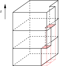
Figure 6: Loops can change their shapes and move in space like amoebas, by absorbing or emitting small loops.

As a result of the gauge symmetry, there is no quadratic hopping term for loops in the Hamiltonian. However, this does not necessarily mean that loops are always localized in space. Loops can change their shapes and move in space by absorbing or emitting other loops. For example, Fig. 6 shows a loop changing its shape by absorbing two small loops. Therefore, loops can propagate with the help of other loops. If loop fields are ‘condensed’, whose precise meaning will become clear in a moment, the condensate provides a coherent background on which other loops can propagate. Loops propagate ‘on the shoulders of other loops’ to explore the bulk space. This is analogous to the the slave-particle theory discussed in Sec. II. One difference is that loop fields themselves play the role of ‘hopping fields’ for other loops, while in slave-particle theory the hopping field is a bi-linear of slave-particle fields. The difference originates from the fact that loops are extended objects while slave-particles are point objects. Only when the condensates of loop fields are ‘coherent’, the bulk space is regarded as a well defined extended space by loops. Otherwise, loops are more or less localized in space. In this sense, an extended space emerges in the bulk as a dynamical feature of a phase where loop fields form coherent condensates.

When do loop fields become coherent ? To make this notion more precise, we first note that the phase modes of complex loop fields $\phi_{C}=|\phi_{C}|e^{ib_{C}}$ play the role of the spatial components of the two-form gauge field. To see this, suppose that the loop field has a background value $<\phi_{C}>$. Then the cubic interaction generates a quadratic hopping term,

$$\displaystyle-\frac{\alpha<\phi_{C}>}{M^{2}}a_{C+C^{{}^{\prime}}}^{\dagger}a_{C^{{}^{\prime}}}.$$ (55)

The amplitude of $<\phi_{C}>$ is the strength of the hopping, and the phase determines the geometric phase acquired when the loop $C^{{}^{\prime}}$ hops to $C^{{}^{\prime}}+C$. Therefore $b_{C}$ plays the role of the spatial components of the two-form gauge field to which loops are electrically coupled. Note that the two-form gauge field is also a part of dynamical loop fields. We identify

$$\displaystyle b_{C}=\int_{A_{C}}B,$$ (56)

where $B_{\mu\nu}$ is the spatial components of the two-form gauge field and the integration is over an area $A_{C}$ enclosed by the loop $C$. Let us focus on the loops with unit plaquettes in which case we take $A_{C}$ as the surface spanned by the unit plaquette.

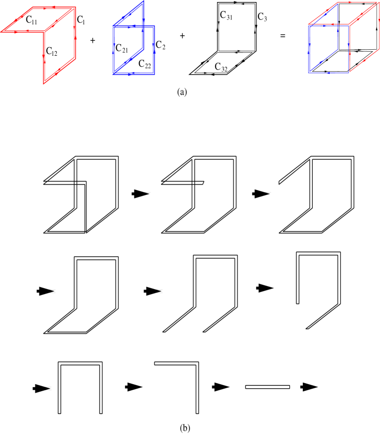
Figure 7: Kinetic energy for the two-form gauge field generated by heavy loop fields. (a) Three vertices each of which involves one loop with length $6$ and two loops with length $4$ can generate a term for the six loops with length $4$, once the loop fields with length $6$ are integrated out. The resulting term for the small loops becomes the kinetic energy for the two-form gauge field. (b) In integrating out the loop fields with length $6$ in (a), one has to introduce a series of nine vertices. Each step depicts a process of adding a new vertex and integrating out one or two loop fields : two fields for the first and the fourth steps, and one loop field for the other steps.

Although the two-form gauge field does not have the bare action, it acquires the kinetic energy from quantum fluctuations. This is similar to the way that the Maxwell’s term is dynamically generated for the auxiliary gauge field in the slave-particle theory as discussed in Sec. II. The gauge coupling for the two-form gauge field is renormalized to $O(1/N^{2})$. This can be understood by integrating out ‘heavy’ loop fields to obtain an effective action for ‘light’ loop fields in the bulk. It is easiest to see the generation of the kinetic energy in the large $M$ limit, where we can use $1/M$ as an expansion parameter. The ’mass’ of a loop field is proportional to the length of the loop because of the tension. We integrate out loop fields with $L>4$ and obtain an action for the loop fields with $L\leq 4$. In particular, we focus on the effective action for the shortest non-self-retracting loops with $L_{C}=4$ whose phase modes can be viewed as the spatial components of the two-form gauge field on unit plaquettes. For simplicity, we choose the temporal gauge with $B_{\mu z}=0$ and the scale of $z$ to set $\alpha=1$.

Let us consider three vertices in Eq. (52). Each vertex has the form $\frac{N^{2}}{M}\phi_{C_{i}}^{*}\phi_{C_{i1}}\phi_{C_{i2}}$ with $i=1,2,3$, where $C_{i}$’s have length $6$ and $C_{il}$’s with $l=1,2$ have length $4$ as is represented in Fig. 7 (a). They describe the processes where a loop on a unit plaquette with sides $\mu,\nu$ merges with a loop on a unit plaquette with sides $\nu,\lambda$ to form a loop with with length $6$. Here we interpret $\phi_{C_{i}}$’s as heavy fields and $\phi_{C_{il}}$’s with $l=1,2$ as light fields. In particular, the phase modes of $\phi_{C_{il}}$ represents the two-form gauge field defined on each plaquette. Now we integrate out the heavy loop fields using the quadratic action. Because this quadratic action has the local $U(1)$ symmetry in the loop space, $\phi_{C}\rightarrow e^{i\varphi_{C}}\phi_{C}$, we need to introduce a series of vertices in order to saturate $\phi_{C}^{*}$ with $\phi_{C}$ and obtain a non-vanishing result. A minimum path to saturate all heavy fields is shown in Fig. 7 (b). In the first step, we add a vertex of the type $\frac{N^{2}}{M^{2}}\phi_{(C_{1}+C_{2})_{ij}}^{*}\phi_{C_{1}}\phi_{C_{2}}$, where $(C_{1}+C_{2})_{ij}$ is a loop that results from merging $C_{1}$ and $C_{2}$ by removing one shared bond. Integrating out $\phi_{C_{1}}$ and $\phi_{C_{2}}$, we obtain the loop fields in the second configuration in Fig. 7 (b). In the second step, we use a vertex $\frac{N^{2}}{M^{2}}\phi_{(C_{1}+C_{2})_{ij}^{{}^{\prime}}}^{*}\phi_{(C_{1}+C_{2})_{ij}}$, and integrate out $\phi_{(C_{1}+C_{2})_{ij}}$. In this step, the merged loop in the first step become a shorter loop $(C_{1}+C_{2})_{ij}^{{}^{\prime}}$ by eliminating one self-retracting link. The remaining steps can be understood in a similar way. In total, nine vertices and eleven loop propagators are needed. (Note that each of the first and fourth steps introduces two propagators because two loop fields are integrated out in those steps, while all the others involve only one propagator.) Each vertex contributes $\frac{N^{2}}{M^{2}}$ and each propagator contributes $\frac{1}{N^{2}}$. Combined with the factor $\left(\frac{N^{2}}{M^{2}}\right)^{3}$ from the original three vertices, we obtain an action for the light loop fields,

$$\displaystyle S_{eff}\sim-\int dz\sum_{\mbox{cubes}}\frac{N^{2}}{M^{24}}\left[\prod_{i=1}^{3}\phi_{C_{i1}}\phi_{C_{i2}}+\prod_{i=1}^{3}\phi_{\bar{C}_{i1}}\phi_{\bar{C}_{i2}}\right],$$ (57)

where the summation is over all cubes in the $D$-dimensional lattice. The second term is from the same process for the anti-loops. The loop field for the anti-loop, $\phi_{\bar{C}}$ is in priori independent of $\phi_{C}$. However they are dynamically mixed. Because of pair-annihilation and pair-creation processes of loops and anti-loops as is shown in Fig. 4, the effective action should include terms of the form, $\phi_{C}\phi_{\bar{C}}$ and $\phi_{C}^{*}\phi_{\bar{C}}^{*}$. As a result, the phase modes of $\phi_{C}$ and $\phi_{\bar{C}}$ are locked. Only the anti-symmetric mode with $b_{\bar{C}}=-b_{C}$ remains gapless in the presence of mixing. If $\phi_{C_{il}}$’s have finite amplitude $\phi_{0}$, this gives the standard ‘magnetic’ term for the two-form gauge field defined on each cube of the lattice

$$\displaystyle-\frac{1}{g_{KR}^{2}}\int dz\sum_{\mbox{cubes}}\cos\left[a^{3}(\Delta_{\mu}B_{\nu\lambda}+\Delta_{\nu}B_{\lambda\mu}+\Delta_{\lambda}B_{\mu\nu})\right],$$ (58)

where we use the fact that $b_{\Box}=a^{2}B_{\mu\nu}$ for a unit plaquette with sides $\mu$, $\nu$. The finite derivative is defined as $\Delta_{\mu}B_{\nu\lambda}\equiv\frac{B_{\nu\lambda}(x+\hat{x}^{\mu})-B_{\nu\lambda}(x)}{a}$. Here $g_{KR}^{2}\sim\left[\frac{N^{2}}{M^{24}}\phi_{0}^{6}\right]^{-1}$ is the renormalized coupling for the Kalb-Ramond (KR) two-form gauge field.

Now we turn our attention to the ‘electric’ term which involves the time-derivative of the gauge field. We consider the quadratic action for the loop fields on unit plaquettes,

$$\displaystyle N^{2}\left[\phi_{C}^{*}(\partial_{z}+L_{C})\phi_{C}+\phi_{\bar{C}}^{*}(\partial_{z}+L_{\bar{C}})\phi_{\bar{C}}\right].$$ (59)

If we integrate out the amplitude fluctuations of the loop fields, the time derivative term will be generated for $b_{C}$. Because of the dynamical constraint $b_{\bar{C}}=-b_{C}$ caused by the mixing between $\phi_{C}$ and $\phi_{\bar{C}}$, the linear time derivative term is canceled, leading to the second derivative term,

$$\displaystyle N^{2}a^{4}\int dz\sum_{\Box}(\partial_{z}B_{\mu\nu})^{2}$$ (60)

for each plaquette. Eqs. (58) and (60) represent the full kinetic energy term for the two-form gauge field in the temporal gauge.

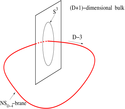
Figure 8: An $NS_{D-4}$-brane in the $(D+1)$-dimensional space. Around an $NS_{D-4}$-brane, there is a net flux of $2\pi$ for the three-form flux : $\int_{S^{3}}H=2\pi$. When the tension of the $NS_{D-4}$-brane is positive, $NS_{D-4}$-branes generated out of quantum fluctuations remain small. When the tension becomes negative, $NS_{D-4}$-branes are proliferated in the bulk.

Because of the gauge symmetry, the mass term is not allowed for the two-form gauge field in the bulk. However, the gauge symmetry does not automatically imply that the two-form field arises as a massless excitation in the bulk. This is because of the compactness of the phase mode : $b_{C}\sim b_{C}+2\pi$, which allows for a topological defect to exist as a magnetic excitation of the gauge field. In the presence of topological defects, the field strength $H=dB$ does not satisfy the Bianchi identity $dH=0$. In $(D+1)$-dimensional space-time, the topological defect which carries a magnetic charge is a $(D-4)$-brane, which is a $(D-3)$-dimensional object in space-time. We call this object $NS_{D-4}$ brane. Around the $NS_{D-4}$-brane, there is a net $2\pi$ flux for the three-form flux,

$$\displaystyle dH(x)=2\pi\int d\xi^{D-3}\delta^{D+1}(x-\xi),$$ (61)

where $\xi$ is the coordinate of the NS-brane embedded in the $(D+1)$-dimensional space, and $d\xi^{D-3}$ is the oriented volume element of the brane. This is illustrated in Fig. 8. Note that the Dirac quantization condition between the charge carried by loop fields, which is set to be $1$ as can be seen from Eq. (49), and the charge of the $NS_{D-4}$-brane is automatically satisfied. This follows from the fact that the phase $2\pi$ on a unit plaquette is invisible to loop fields. In $D>4$, this is a brane extended along $(D-4)$-directions in space at a given time slice with fixed $z$. In $D=4$, this is a point-like particle. In $D=3$, this is an instanton which is localized both in space and time. Whether loop fields provide a coherent background for other loops is determined by dynamics of $NS_{D-4}$-branes.

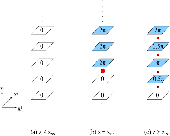
Figure 9: An $NS_{D-4}$-brane can be viewed as an instanton in $D=3$ where one inserts a source of $2\pi$ magnetic charge to the theory at a given $z_{NS}$. (a) For $z<z_{NS}$, the phases of loop fields are zero. (b) At $z=z_{NS}$, the phases of loop fields are $2\pi$ along a semi-infinite line creating a cube which contains the 3-form flux of $2\pi$ : $H_{123}=\Delta_{1}B_{23}+\Delta_{2}B_{31}+\Delta_{3}B_{12}=\frac{2\pi}{a^{3}}\delta_{x,x_{NS}}$. (c) For $z>z_{NS}$ the configuration in (b) is smoothly deformed and the flux is smeared over a region which contains the net flux $2\pi$. The size of red dots represents the amount of 3-form flux contained in each cube.

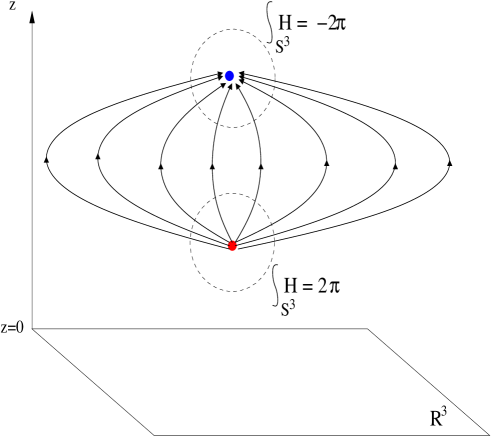
Figure 10: A pair of instanton and anti-instanton in the four-dimensional bulk for $D=3$.

The physical nature of $NS_{D-4}$-brane can be most easily understood in $D=3$ where $NS_{D-4}$-brane is an instanton localized at a point in the four-dimensional bulk. We start with a configuration of the loop fields $\phi_{\Box}$ for unit plaquettes with

$$\displaystyle b_{\Box_{12}}(x,z) = 2\pi\delta_{x^{1},x^{1}_{NS}}\delta_{x^{2},x^{2}_{NS}}\Theta(x^{3}-x^{3}_{NS})\Theta(z-z_{NS}),$$ (62)

where the phases of the loop fields on $x^{1}-x^{2}$ plaquettes are $2\pi$ along a semi-infinite line in the $3$-dimensional space for $z>z_{NS}$, and the phases are zero, otherwise. Since $b_{C}\equiv b_{C}+2\pi$, this configuration is equivalent to the trivial configuration where $b_{C}=0$ everywhere. However, we can view this configuration as a topological defect with a non-trivial three-form flux on a cube, $H_{123}=2\pi\delta^{3}(x-x_{NS})\Theta(z-z_{NS})$. This means that there is a source of magnetic flux for the two-form gauge field localized at a point in the bulk, $dH=2\pi\delta^{3}(x-x_{NS})\delta(z-z_{NS})$. Since $2\pi$-magnetic flux is concentrated at one cube, the topological defect is trivial. Now the configuration is deformed smoothly, $b_{C}^{{}^{\prime}}=b_{C}+\delta b_{C}$. Under a smooth deformation, the flux is smeared out over an extended region in the space, while the net flux $2\pi$ does not change. Now the flux is visible by loop fields. This is illustrated in Fig. 9. As $z$ is increased further, the flux can merge back into one cube and disappear into the vacuum through the inverse process. This describes a pair of instanton and anti-instanton as is shown in Fig. 10. In higher dimensions, $NS_{D-4}$-branes are extended objects. In $(D+1)$-dimensional bulk, we can think of Fig. 10 as a configuration in a slice at a fixed $x^{5},...,x^{D+1}$, where the $NS_{D-4}$-brane is extended along the $(D-3)$ directions. They can be wrapped into compact objects as is shown in Fig. 8, which in a sense describe bound states of $NS_{D-4}$-brane and anti-$NS_{D-4}$-brane. If the size of the wrapped $NS_{D-4}$-branes become infinite, $NS_{D-4}$-brane and anti-$NS_{D-4}$branes become unbound.

The tension of the $NS_{D-4}$-brane is proportional to $N^{2}$ because $NS_{D-4}$-brane is a topological defect of the two-form gauge field with the coupling proportional to $1/N^{2}$. Here we are using the term ‘tension’ in a loose sense. In $D>4$, it literally means the tension of $NS_{D-4}$-branes. In $D=4$, it refers to the mass of ‘$NS_{D-4}$-particle’. In $D=3$, it refers to the action of ‘$NS_{D-4}$-instanton’. For a sufficiently large $N$, we expect that $NS_{D-4}$-branes are gapped. In this case, $NS_{D-4}$-branes will be wrapped into compact objects with a finite size in the vacuum. For a small $N$, the bare tension of $NS_{D-4}$-brane is small, and quantum fluctuations can renormalize the tension into a negative value. Then $NS_{D-4}$-branes are condensed, and extended $NS_{D-4}$-branes fill the space in the bulk. It is also possible that $NS_{D-4}$-branes always condense for any finite $N$ in low dimensions. We will discuss the consequences of different dynamics of $NS_{D-4}$-branes in the following section.

VII Emergent space and quantum order in Holographic phases

In this section, we will discuss various phases that the matrix model can have, by focusing on the behavior of $NS_{D-4}$-branes. In particular, we will see that the dynamics of string excitations around a saddle-point configuration of the loop fields is determined by the fate of $NS_{D-4}$-branes in the bulk. In order to discuss about this issue systematically, we first turn to the saddle point equations.

VII.1 Saddle point solution

The saddle point configuration of loop fields is determined from the equation of motion.

$$\displaystyle\partial_{z}\phi_{C} = -L_{C}\phi_{C}+\frac{1}{M^{2}}\left(2F_{ij}[C,C_{1}]\phi_{C_{1}}^{*}\phi_{[C+C_{1}]_{ij}}+G_{ij}[C_{1},C_{2}]\phi_{C_{1}}\phi_{C_{2}}\delta_{(C_{1}+C_{2})_{ij},C}\right),$$ (63)

$$-\partial_{z}\phi_{C}^{*} = -L_{C}\phi_{C}^{*}+\frac{1}{M^{2}}\left(F_{ij}[C_{1},C_{2}]\phi_{C_{1}}^{*}\phi_{C_{2}}^{*}\delta_{[C_{1}+C_{2}]_{ij},C}+2G_{ij}[C_{1},C_{2}]\phi_{(C+C_{1})_{ij}}^{*}\phi_{C_{1}}\right).$$ (64)

These equations are supplemented by two sets of boundary conditions. It is more convenient to use the action with discrete time step $dz$ to isolate boundary fields from bulk fields. The UV boundary condition is obtained from Eq. (12),

$$\displaystyle\frac{\partial S_{1}}{\partial\phi^{(0)*}_{C}}=N^{2}\left[\phi_{C}^{(0)}+\frac{\partial V[\phi_{C}^{(0)*}]}{\partial\phi^{(0)*}_{C}}\right]=0,$$ (65)

and the IR boundary condition from Eq. (29),

$$\displaystyle\frac{\partial S_{7}}{\partial\phi^{(R)}_{C}}=N^{2}\left[\phi_{C}^{(R)*}+\frac{\partial V^{{}^{\prime}}[\phi_{C}^{(R)}]}{\partial\phi^{(R)}_{C}}\right]=0.$$ (66)

When the UV potential includes only single-trace operators, $V=-J_{C}\phi_{C}^{(0)*}$, Eq. (65) leads to the standard Dirichlet boundary condition for the source field : $\phi^{(0)}_{C}=J_{C}$. For more general non-linear UV potential, it becomes a mixed boundary condition. This is consistent with the prescription for the UV boundary condition in the presence of multi-trace deformations in the standard AdS/CFT dictionaryWITTEN_multi . The IR boundary condition is a mixed one because $V^{{}^{\prime}}$ is in general non-linear. For self-retracting loops, $V^{{}^{\prime}}$ also contains terms that are linear in loop fields as is shown in the first term in Eq. (32). Eq. (66) then implies that $\phi_{C}^{*}\neq 0$ at the IR boundary for self-retracting loops. As will be shown in the next paragraph, this means that loop fields for self-retracting loops have non-zero expectation values at all $z$ in the bulk. This, in turn, generates non-zero vacuum expectation values of the source fields $\phi_{C}$ for self-retracting loops. As was discussed in Fig. 4, self-retracting loops can turn into a loop/anti-loop pair through an interaction.

In general, the saddle point configuration is $z$-dependent, and $\phi_{C}(z)$ is not necessarily the complex conjugate of $\phi_{C}^{*}(z)$. One should treat $\phi_{C}$ and $\phi_{C}^{*}$ as two independent fields. Then the equations of motion can be viewed as a set of Hamiltonian equations in the phase space of $\{\phi_{C},\phi_{C}^{*}\}$.

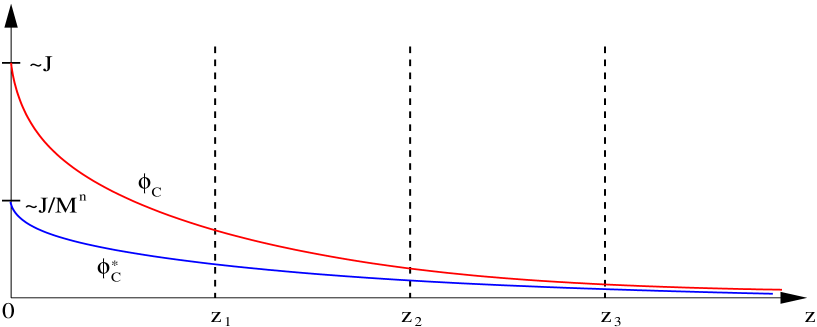
Figure 11: A schematic profile of a loop field $\phi_{C}$ and the conjugate field $\phi_{C}^{*}$ in a deep confinement phase. $\phi_{C}$ and $\phi_{C}^{*}$ satisfy the boundary condition given by Eq. (67) at any $z$ in the bulk.

Although Eqs. (63) and (64) are coupled equations for $\phi_{C}$ and $\phi_{C}^{*}$, one can eliminate $\phi_{C}^{*}$ in favor of $\phi_{C}$. We first note that the partition function and all observables including vacuum expectation values of Wilson loop operators represented by $\phi_{C}^{*}(0)$ are independent of how we choose $\beta$ in Eqs. (34) and (35). This means that the saddle point solution $\phi_{C}(z)$ and $\phi_{C}^{*}(z)$ for $z<\beta$ is independent of $\beta$. Since we could have put $\beta$ anywhere, $\phi_{C}$ and $\phi_{C}^{*}$ should satisfy the IR boundary condition at any $z$,

$$\displaystyle\phi_{C}^{*}(z)=-\frac{\partial V^{{}^{\prime}}[\phi_{C}(z)]}{\partial\phi_{C}(z)}.$$ (67)

This is illustrated in Fig. 11. The fact that one can put the IR boundary at any $z$ has an interesting implication on the role of the IR boundary. Usually, one can associate a boundary condition with a physical object located at the boundary. However, Eq. (67) is special in the sense that an observer at $z<\beta$ can not ‘feel’ the presence of a physically identifiable object at $z=\beta$. Suppose one stops the renormalization group procedure at $z=\beta$ and impose Eq. (67) at the IR boundary. If a UV observer sends a wave toward the IR region, the reflected wave from the IR region is exactly the same as the reflected wave one would observe in the space which is extended to $z=\infty$ without an boundary. In this sense, the IR boundary is not a physical boundary : one can always trade the IR boundary with the space where $z$ is extended to infinity.

Using Eq. (67), we can write a set of first order differential equations for the source field only,

$$\displaystyle\partial_{z}\phi_{C} = -L_{C}\phi_{C}+\frac{1}{M^{2}}\left(-2F_{ij}[C,C_{1}]\frac{\partial V^{{}^{\prime}}[\phi_{C_{1}}]}{\partial\phi_{C_{1}}}\phi_{[C+C_{1}]_{ij}}+G_{ij}[C_{1},C_{2}]\phi_{C_{1}}\phi_{C_{2}}\delta_{(C_{1}+C_{2})_{ij},C}\right).$$

Once $\phi_{C}(z)$ is solved using the UV boundary condition in Eq. (65), the conjugate field is readily determined from Eq. (67). One can check that the source and the conjugate field satisfy Eq. (67) at all $z$ through an explicit calculation perturbatively in $1/M$ (see Appendix C).

It is tempting to interpret Eq. (LABEL:EOM1_2) as the beta function of the sources for Wilson loop operators. However, there is an important caveat for this interpretation, which comes from the fact that this is the saddle point equation of the quantum theory for dynamical loop fields. The saddle point equation is expected to be valid only when quantum fluctuations are weak for a sufficiently large $N$. For a small $N$, one can still have a well-defined beta function under the usual renormalization group flowPOLCHINSKI84 ; POLONYI . However, the beta function can not be directly identified with the saddle point equation of the loop fields if the saddle point solution becomes unstable by strong quantum fluctuations. As we will see in the following sections, non-perturbative fluctuations can invalidate the holographic description for small $N$.

VII.2 Fluctuations near the saddle point

Fluctuations near the saddle point configuration $\bar{\phi}_{C}(z)$ describes dynamical string in the bulk,

$$\displaystyle\phi_{C}(z) = \bar{\phi}_{C}(z)+\chi_{C}(z),$$ (69)

where $\chi_{C}$ describes small fluctuations around the saddle point. We call $\chi_{C}$ string field to distinguish it from the loop field $\phi_{C}$. The dynamics of string is governed by the action,

$$\displaystyle S_{bulk} = N^{2}\int_{0}^{\beta}dz\Bigl{[}\chi_{C}^{*}\partial_{z}\chi_{C}+L_{C}\chi_{C}^{*}\chi_{C}$$ (70)

$$-\frac{1}{M^{2}}\Bigl{(}F_{ij}[C_{1},C_{2}]\bar{\phi}_{[C_{1}+C_{2}]_{ij}}(z)\chi_{C_{1}}^{*}\chi_{C_{2}}^{*}+2F_{ij}[C_{1},C_{2}]\bar{\phi}_{C_{1}}^{*}(z)\chi_{[C_{1}+C_{2}]_{ij}}\chi_{C_{2}}^{*}$$

$$~{}~{}~{}~{}~{}~{}+G_{ij}[C_{1},C_{2}]\bar{\phi}_{(C_{1}+C_{2})_{ij}}^{*}(z)\chi_{C_{1}}\chi_{C_{2}}+2G_{ij}[C_{1},C_{2}]\bar{\phi}_{C_{1}}(z)\chi_{C_{2}}\chi_{(C_{1}+C_{2})_{ij}}^{*}\Bigr{)}$$

$$-\frac{1}{M^{2}}\Bigl{(}F_{ij}[C_{1},C_{2}]\chi_{[C_{1}+C_{2}]_{ij}}\chi_{C_{1}}^{*}\chi_{C_{2}}^{*}+G_{ij}[C_{1},C_{2}]\chi_{C_{1}}\chi_{C_{2}}\chi_{(C_{1}+C_{2})_{ij}}^{*}\Bigr{)}\Bigr{]}.$$

Here $\chi_{C}(z)=\chi_{C}^{r}(z)+i\chi_{C}^{i}(z)$ is a complex field. Following the standard method of the steepest descent, the contours of the real and imaginary parts of the complex fields are chosen so that the real part of the eigenvalues of the quadratic action becomes maximum along the deformed contoursCALLAN_COLEMAN ; REINHARDT . Note that the string fields $\chi_{C}$ acquire the hopping term through non-zero condensates of loop fields. It also has the terms that describe pair creation/annihilation of two closed strings.

VII.3 Possible phases of the matrix model

In this section, we describe possible states of the matrix model using the holographic description. In particular, we will see that strings have different dynamics depending on the behavior of $NS_{D-4}$-branes. One observable that is useful in distinguishing different states is the correlation function between Wilson loop operators. In particular, we focus on the correlation function of phase fluctuations of Wilson loop operators,

$$\displaystyle F(C,C^{{}^{\prime}}) = \left<\delta b_{C}\delta b_{C^{{}^{\prime}}}\right>,$$ (71)

where $\delta b_{C}=b_{C}-<b_{C}>$. In the bulk description, this correlation function corresponds to a two-point string-string correlation function. This object is of particular interest because the string state that corresponds to the phase mode describes the two-form gauge field in the bulk.

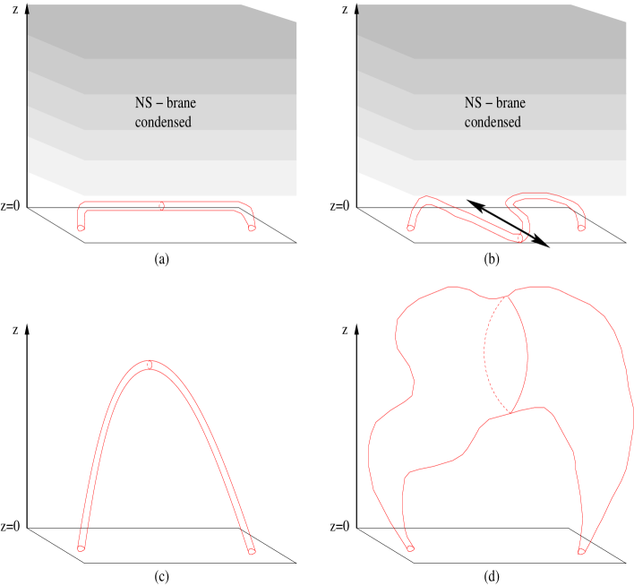
Figure 12: The Wilson loop correlation function in different phases. (a) In the confinement phase, $NS_{D-4}$-branes are condensed in the bulk, and the string emitted at the boundary stays near the boundary. Due to weak fluctuations of string world sheet, the string propagates in a straight path. (b) In the non-holographic critical phase, $NS_{D-4}$-branes remain condensed in the IR region. However, large amplitudes of loop fields in the UV region make the string world sheet highly fluctuating along the $D$ dimensions. As a result, the correlation function decays algebraically. (c) In the holographic critical phase, loop fields acquire finite expectation values everywhere in the bulk, and $NS_{D-4}$-brane is gapped. Strings can propagate deep inside the bulk, and the correlation function shows a power-law behavior with a scaling dimension determined by the mass of the string. (d) In the deconfinement phase, loop fields with infinitely large loops acquire non-zero expectation value in the bulk. This causes highly non-local fluctuations of the world sheet of a string in the bulk.

VII.3.1 Confinement phase

For non-self-retracting loops, $V^{{}^{\prime}}$ is quadratic or of higher order in the loop fields. For small $\phi_{C}(0)$, the first term on the right hand side of Eq. (LABEL:EOM1_2) dominates. As a result, $\phi_{C}(z)$ decays exponentially in $z$. Because larger loops for which sources are not turned on at the UV boundary are generated out of many small loops, amplitudes with larger loops decay exponentially with the area enclosed by the loop. This corresponds to the confinement phase of the matrix model. In the confinement phase, one can define a cross-over scale $z^{*}$ beyond which loop fields have negligible amplitudes.

Now let us consider dynamics of strings in the IR ($z>z^{*}$) and the UV ($z<z^{*}$) regions separately. In the deep IR region, amplitudes of non-self-retracting loop fields are exponentially small. This means that loops that are emitted from the UV boundary rarely reach the IR region. In this region, phase fluctuations of loop fields do not have a stiffness, which leads to a condensation of $NS_{D-4}$-branes. As a result, strings are subject to the strongly fluctuating two-form gauge field. In this region, strings are confined, and the two-form gauge field is gappedPOLYAKOV87 ; REY1991 . For a more systematic discussion on possible phases of anti-symmetric fields, see Ref. QUEVEDO . In the deep IR region, strings can not propagate by themselves; only charge neutral bound states of string and anti-string can propagate. On the other hand, loop fields have significant amplitudes in the UV region. The source field $J_{\{C_{1},..,C_{n}\}}$ plays the role of a symmetry-breaking field at the UV boundary. As a result, phase fluctuations of loop fields are small, and $NS_{D-4}$-branes are suppressed in the UV region. Because loop fields are coherent near the UV boundary, strings are deconfined in this region. There is a domain wall that separates the IR region with condensed $NS_{D-4}$-brane and the UV region without $NS_{D-4}$-brane.

In the confinement phase, a string that is emitted from the boundary can not penetrate through the wall of condensed $NS_{D-4}$-brane. Therefore it stays within the UV region. Deep inside the confinement phase with small $J_{\{C_{1},..,C_{n}\}}$, the condensates of loop fields are small. As a result, the hopping amplitudes of strings are small, and fluctuations of string world sheet is small. For the correlation function in Eq. (71), the strings inserted at the UV boundary are connected through a minimum number of hoppings, forming a straight path as is shown in Fig. 12 (a). This leads to an exponentially decaying correlation function for the Wilson loop operators. In the confinement phase, the bulk geometry ends at a finite scale due to the proliferation of $NS_{D-4}$-branes. This is reminiscent of the idea that geometry can get truncated by tachyon condensationHS2006 .

As $J_{\{C_{1},..,C_{n}\}}$ is dialed up, amplitudes of loop fields in the bulk increase. Accordingly the cross-over scale $z^{*}$ increases. At the same time, fluctuations of string world sheet increase as the amplitudes of loop fields become larger. Suppose the system becomes critical either by fine tuning or dynamical tuning. In the case of fine tuning, one may have to tune more than one microscopic parameters to reach a critical point. For the following discussions which focus on physical properties of the critical states, it is not important whether those states are realized as phases or critical points. So we will use the term ‘critical phase’ in a broad sense to include not only critical phases realized within a finite region in the parameter space of a microscopic model but also critical states realized at critical points by fine tuning. Logically, there exist at least two different scenarios via a criticality is achieved. In the first scenario, $NS_{D-4}$-branes remain condensed in the IR region with a finite $z^{*}$. But loop fields acquire large amplitudes in the UV region so that strings are delocalized along the $D$-directions, mediating critical correlations between operators inserted on the UV boundary. In the second scenario, the cross-over scale diverges and $NS_{D-4}$-branes are suppressed out in the bulk. In this case, strings can propagate deep inside the bulk. In the following, we will discuss the two scenarios in more detail.

VII.3.2 Non-holographic critical phase

Here we discuss the first case which is likely to be realized when $N$ is small. For a small $N$, $NS_{D-4}$-branes are ‘light’. Even though loop fields have finite amplitudes in the bulk, quantum fluctuations may destabilize the saddle-point solution. Indeed this is what always occurs in the pure 2-form gauge theory in the flat four dimensional spacePOLYAKOV87 ; ORLAND82 ; PEARSON . If the mass or tension of $NS_{D-4}$-brane becomes negative, $NS_{D-4}$-branes are condensed. Once $NS_{D-4}$-branes are proliferated, the two-form gauge field acquires a mass gap, and strings are confined in the bulk, as is the case in the confinement phase. The difference from the confinement phase is that the boundary theory is critical. The boundary theory can be critical although strings are confined deep inside the bulk because critical correlation between boundary fields can be mediated by strings that propagate near the UV region. It is noted that ‘confinement’ in the boundary matrix model and ‘confinement’ of strings in the bulk are not the same thing. In this phase, strings are confined in the bulk, but the matrix model is not in the confinement phase. We call this non-holographic critical phase.

In this critical phase, a string emitted from the UV boundary no longer takes the straight path because of large amplitudes of background loop fields in the UV region. Rather, the world sheet of string strongly fluctuates, and the correlation function can decay in a power law because of delocalized strings. However, strings are still localized within the UV region along the $z$ direction due to the condensation of $NS_{D-4}$-branes in the IR region. The fluctuations of the world sheets of strings is predominantly along the $D$ space dimensions as is illustrated in Fig. 12 (b).

VII.3.3 Holographic critical phase I : deconfined closed string

The second scenario is qualitatively different from the previous one. In this phase, loop fields develop non-zero amplitudes in the IR region. For a sufficiently large $N$, $NS_{D-4}$-branes are suppressed, and the saddle-point solution is stable against non-perturbative fluctuations of the two-form gauge field. If $NS_{D-4}$-branes are suppressed, the compactness of the gauge field is unimportant at long distances. Strings are deconfined in the bulk because loop fields provide a background in which strings can propagate coherently. Note that strings are still coupled with the dynamical two-form gauge field, but the gauge field is no longer confining in this phase. This is analogous to the Coulomb phase discussed in Sec. II. Thanks to the coherent background loop fields, closed strings can explore the extended space in the bulk. The bulk space is not a gauge invariant object. However, it assumes a ‘classical identity’ in the large $N$ limit where fluctuations of loop fields are suppressed. In this sense, the bulk space emerges in the holographic phase, but not in the non-holographic phase.

Because of the source that explicitly breaks the gauge symmetry, the transformation $B_{MN}\rightarrow B_{MN}+\partial_{M}\theta_{N}-\partial_{N}\theta_{M}$, is not a symmetry at the UV boundary. As a result, the $U(1)$ mode $\theta_{M}$ becomes a physical mode. This means that there is a $U(1)$ gauge field localized at the UV boundary in the dual theory. This $U(1)$ mode originates from the Abelian component of the $U(N)$ matrix theory. We identify this as the singleton mode localized at the boundaryWITTEN ; Aharony_Witten98 ; Maldacena2001 .

It is noted that the symmetry breaking source $J_{\{C_{1},..,C_{n}\}}$ at the UV boundary does not necessarily open up a gap for the phase modes of loop fields in the bulk. This is because the symmetry breaking source is only at the UV boundary, but not in the bulk. This is analogous to the case where one applies a symmetry breaking field at the boundary of a system where a global symmetry is spontaneously broken in the bulk. Although the boundary field determines the direction of the symmetry breaking in the whole system, the Goldstone mode in the bulk survives in the thermodynamic limit.

The dynamics of the $D$-dimensional matrix model in the long distance limit is governed by strings that propagate in the $(D+1)$-dimensional space. We call this phase holographic phase. The hallmarks of the holographic phase are deconfined strings that propagate in the bulk with the extra dimension and the emergence of the Bianchi identity $dH=0$ for the two-form gauge field in the long distance limit. It is emphasized that these features are not protected by any symmetry of the original matrix model. They are dynamical properties which emerge only in the holographic phase. The quantum order present in the holographic phase is analogous to the quantum order associated with the emergent Bianchi identity in the fractionalized phase of the slave-particle theory as discussed in Sec. II.

In the holographic critical phase, strings can propagate deep inside the bulk as is shown in Fig. 12 (c). The correlation function shows a power-law decay through a classical trajectory that is extended to the bulk. Because of the gauge symmetry and the non-trivial quantum order, we expect that the scaling dimension of the phase mode of Wilson loop operators will be protected accordingly. To determine the scaling dimension, one has to first solve the loop equations in the bulk and find the string Green’s function in the background determined by the loop fields. We defer an explicit calculation for future studies.

In the four-dimensional ${\cal N}=4$ super Yang-Mills theory, the phase mode of Wilson loop operators has the scaling dimension $6$DAS98 . The reason why it is not $2$, which is the expected scaling dimension for massless two-form fields in $D=4$WITTEN , is that a Chern-Simons coupling generates a mass for the two-form gauge field through the mixing with the Ramond-Ramond fields. However, the scaling dimension is still protected from acquiring a large quantum correction in the large $N$ limit. Such protection of scaling dimension is often attributed to supersymmetry. However, the non-trivial quantum order will protect the scaling dimension of the phase mode from acquiring a large quantum correction even in non-supersymmetric holographic critical phases in the large $N$ limit. This is true whether or not the two-form gauge field becomes massive through a Chern-Simons coupling with Ramond-Ramond fields. This is because the string theory becomes classical in the large $N$ limit, and the coefficient of the Chern-Simons term is quantized. Therefore the mass of the two-form gauge field can not become large even when other string modes become very massive at strong coupling of the boundary matrix model. This, in turn, implies that the scaling dimension remains small for the phase mode of Wilson loop operators. This is in sharp contrast to the non-holographic critical phase where it is expected that the operator generally receives a large quantum correction at strong coupling.

VII.3.4 Deconfinement phase

Strictly speaking, the critical phases discussed in the previous two sections are kinds of deconfinement phases. Here we use the term ’deconfinement phase’ in a narrower meaning, that is, free theory in the IR limit. If the sources at the boundary are very large, the second and third terms in Eq. (LABEL:EOM1_2) dominate, and the source fields will grow as $z$ increases for $D>4$ in which case the boundary matrix model is expected to flow into IR free gauge theory in the weak coupling (large $J_{\{C_{1},..,C_{n}\}}$) limit. As the amplitudes of the loop fields become larger, large loops are generated through the joining processes. As a result, loop fields with all sizes are condensed in the bulk. Then strings propagating in the bulk become highly non-local because strings can hop from one configuration into another configuration which is very different from the initial one. This is a string condensed phase. In this phase, the two-form gauge field acquires a mass and $NS_{D-4}$-brane is confined due to the Higgs mechanismREY89 ; YI99 .

In the deconfinement phase, a string emitted from the boundary becomes very large in the bulk and lose its identity as a closed string. The critical fluctuations are mediated by highly non-local fluctuations in the bulk. In this phase, the locality is lost in the bulk.

The deconfinement phase can be viewed as an extreme limit of the holographic critical phase discussed in the previous section. Even in the holographic critical phase, some loop fields are condensed in the bulk, as is the case in the deconfinement phase. The difference is that only small loops are condensed in the holographic critical phase while loops with all sizes are condensed in the deconfinement phase. Note that condensations of small loops do not generate a mass gap for the two-form gauge field. This is because closed strings with finite sizes as point-like particles are coupled only with the field strength tensor of the two-form gauge field. In certain models, one can in principle change microscopic parameters to tune the size of condensed loops, smoothly interpolating between the holographic critical phase and the deconfinement phase. This basically controls the size of strings in the bulk. The ${\cal N}=4$ SU(N) gauge theory in four dimensions is believed to be in this class : for a sufficiently large $N$, one can smoothly tune the ’t Hooft coupling $\lambda$ from a large value to zero without going through a phase transition. The one parameter family of the critical theories form a line of fixed points. Here, $\lambda=0$ is a special point where the size of string diverges. In non-supersymmetric theories, it is expected to be harder to stabilize a theory at an arbitrary gauge coupling. Most likely, we expect that the holographic critical phase will arise as a multi-critical point between the confinement phase and the deconfinement phase for a sufficiently large $N$.

VII.4 A mean-field description

Some features of the phases discussed in the previous section can be easily understood if we focus on a subspace within the space of loop fields $\{\phi_{C}\}$. We focus on the mean-field AnsatzREY89 ; YI99 where a loop field is represented by a product of link fields along the loop,

$$\displaystyle\phi_{C}(z)=\prod_{(i,i+\mu)\in C}\xi_{\mu}(i,z).$$ (72)

Here $\xi_{\mu}(i,z)=\xi_{-\mu}^{*}(i+\mu,z)$ is a complex scalar field defined on the link $i,i+\mu$. This is a huge simplification where we reduce the space spanned by functions defined on loop space into the space spanned by functions defined on the links. Under the gauge transformation, the link variables transform as

$$\displaystyle\xi_{\mu}(i,z)\rightarrow e^{i\theta_{\mu}(i,z)}\xi_{\mu}(i,z).$$ (73)

Therefore, these link fields should be charged with respect to the two-form gauge field. A minimal action for the link field that has the same symmetry as the original loop model is an Abelian-Higgs modelREY89 for the link field,

$$\displaystyle S_{bulk} = -t\sum_{\Box}\left[\xi_{M}(i)\xi_{N}(i+M)\xi_{M}^{*}(i+N)\xi_{N}^{*}(i)e^{-iB_{MN}(i)}+c.c.\right]+\sum_{i,M}V(|\xi_{M}(i)|^{2})$$ (74)

$$-\frac{1}{g_{KR}^{2}}\sum_{\mbox{cubes}}\cos(\Delta_{L}B_{MN}+\Delta_{M}B_{NL}+\Delta_{N}B_{LM}).$$

Here we discretize the $z$ direction, and the action is written in a $(D+1)$-dimensional lattice. The box represents sum over all plaquettes including temporal plaquettes. The link fields $\xi_{z}$ along the temporal directions can be viewed as an auxiliary field that is introduced to keep the two-form gauge symmetry. One can use a continuum description as wellYI99 .

The phase structure of this model is very similar to the one for the Abelian-Higgs model for scalar fields discussed in Sec. II. If $NS_{D-4}$-branes are condensed in the bulk, the link fields are confined. This is what happens in the confinement phase and the non-holographic critical phase discussed in the previous section. The bulk physics alone can not distinguish the confinement phase and the non-holographic critical phase.

If the link fields are condensed, the two-form gauge field acquires a mass due to the Higgs mechanismREY89 ; YI99 . Note that loop fields with arbitrarily large size acquires expectation values in the Higgs phase because loop fields are just products of link fields. This corresponds to the deconfinement phase of the boundary matrix model.

If the link field is gapped and the two-form gauge coupling is small, the theory can be in the Coulomb phase. In this phase, closed strings are deconfined and the two-form gauge field arises as a light mode in the bulk. This corresponds to the holographic critical phase. Note that the loop fields can have finite expectation values even though link fields are gapped in this phase.

VII.5 Holographic critical phase II : deconfined open string

The mean field description discussed in the previous section allows one to understand a yet another new phase of the matrix model. To see this, we first note that the decomposition in Eq. (72) has a U(1) gauge redundancy,

$$\displaystyle\xi_{M}(i)\rightarrow e^{i(\gamma_{i+M}-\gamma_{i})}\xi_{M}(i),$$ (75)

where $\gamma_{i}$ is a U(1) phase defined on each site on the bulk space. Because of this U(1) redundancy, the link field can not have a quadratic hopping term. This is similar to the U(1) gauge redundancy present in the slave-particle theory discussed in Sec. II. One can decouple the quartic term for the link fields using the Hubbard-Stratonovich transformation. The resulting action should include a dynamical compact U(1) gauge field,

$$\displaystyle S_{bulk}^{{}^{\prime}} = -t\sum_{i,M\neq N}\left[\xi_{M}^{*}(i+N)\xi_{M}(i)e^{-i\left[B_{MN}(i)-A_{N}(i+M)+A_{N}(i)\right]}+c.c.\right]$$ (76)

$$-t\sum_{i,M\neq N}\left[\xi_{N}^{*}(i)\xi_{M}(i)e^{-i\left[B_{MN}(i)-A_{N}(i+M)+A_{M}(i+N)\right]}+c.c.\right]$$

$$-t\sum_{i,M\neq N}\left[\xi_{N}(i+M)\xi_{M}(i)e^{-i\left[B_{MN}(i)+A_{M}(i+N)+A_{N}(i)\right]}+c.c.\right]$$

$$+\sum_{i,M}V(|\xi_{M}(i)|^{2})-\frac{1}{g_{KR}^{2}}\sum_{\mbox{cubes}}\cos(\Delta_{L}B_{MN}+\Delta_{M}B_{NL}+\Delta_{N}B_{LM}).$$

Under the gauge transformation in Eq. (75), the U(1) gauge field transforms as usual, $A_{M}(i)\rightarrow A_{M}(i)+\gamma_{i+M}-\gamma_{i}$, and the two-form gauge field is invariant. Eq. (75) implies that the link field $\xi_{M}(i)$ carries U(1) charge $+1$ on one end at site $i+M$ and charge $-1$ on the other end at site $i$. Under the two-form gauge transformation in Eq. (73), the U(1) gauge field transforms as

$$\displaystyle A_{M}(i)\rightarrow A_{M}(i)+\theta_{M}(i).$$ (77)

The first term in Eq. (76) describes a link parallel to the direction $M$ hops along the direction $N$ as is shown in Fig. 13 (a), and the second and third terms describe hoppings where the direction of a link changes as in Fig. 13 (b) and (c).

Figure 13: The figures in (a), (b) and (c) show a ‘particle’ denoted as a thick line defined on the link $<i,i+M>$ hops to the link $<i+N,i+M+N>$, $<i,i+N>$ and $<i+M+N,i+M>$, respectively. The dashed lines represent the paths along which the end points of the link follow to which the U(1) gauge field is electrically coupled.

Although the bare coupling for the U(1) gauge field is infinite, the kinetic term will be generated once high energy fluctuations of the link fields are integrated out, renormalizing the gauge coupling to a finite value. Suppose we are in the holographic critical phase where the link fields are gapped and the two-form gauge field is in the deconfinement phase. The U(1) gauge field can be either in the confinement phase or in the deconfinement phase. If the U(1) gauge field is confining, all open links are joined with each other to form closed loops because there is a linearly confining force between open ends. In this phase, only closed strings are allowed. This is the holographic critical phase I discussed in Sec. VII.C.3. On the other hand, if the U(1) gauge field is in the deconfinement phase, closed strings can get fractionalized into open strings, and open strings arise as deconfined excitations. Closed strings can still exist as a bound state of open strings. In this phase, there is an emergent U(1) gauge field in addition to the two-form gauge field. The two-form gauge field is coupled with the world-sheet of strings and the U(1) gauge field is coupled with boundaries of open strings. Here the gapless U(1) gauge field is protected by a quantum order associated with the emergent Bianchi identity $dF=0$ for the U(1) gauge field in the bulk. Open strings are fractionalized excitations of closed strings.

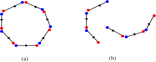
Figure 14: (a) In the confinement phase for the one-form gauge field in the bulk, link fields are always joined to form closed loops, and there exist only closed strings as finite energy states. (b) In the deconfinement phase, closed strings can be fractionalized into open strings. The end points of open strings carry gauge charge for the emergent gauge field in the bulk.

The way open strings and the U(1) gauge field arise as collective excitations of closed string fields is very similar to the way slave-particles emerge as fractionalized excitations along with the emergent U(1) gauge boson in the slave-particle theory discussed in Sec. II. One can go one step further to obtain a different gauge group for open strings. For this we introduce a larger gauge redundancy in Eq. (72),

$$\displaystyle\phi_{C}(z)=\mbox{tr}\left[\prod_{(i,i+\mu)\in C}\Xi_{\mu}(i,z)\right],$$ (78)

where $\Xi_{\mu}(i,z)=\Xi_{-\mu}^{\dagger}(i+\mu,z)$ is a $\tilde{N}\times\tilde{N}$ complex matrix field defined on the link $<i,i+\mu>$ in the bulk. This decomposition has the $U(\tilde{N})$ gauge redundancy,

$$\displaystyle\Xi_{\mu}(i,z)\rightarrow V_{i}^{\dagger}(z)\Xi_{\mu}(i,z)V_{i+\mu}(z).$$ (79)

Therefore the link fields now have to be coupled with a dynamical $U(\tilde{N})$ gauge field in the bulk.

$$\displaystyle S_{bulk}^{{}^{\prime\prime}} = -t\sum_{i,M\neq N}\mbox{tr}\left[\Xi_{M}^{\dagger}(i+N)U_{i+N,i}\Xi_{M}(i)U_{i+M,i+M+N}e^{-iB_{MN}(i)}+c.c.\right]$$ (80)

$$-t\sum_{i,M\neq N}\mbox{tr}\left[\Xi_{N}^{\dagger}(i)\Xi_{M}(i)U_{i+M,i+M+N}U_{i+M+N,i+N}e^{-iB_{MN}(i)}+c.c.\right]$$

$$-t\sum_{i,M\neq N}\mbox{tr}\left[\Xi_{N}(i+M)\Xi_{M}(i)U_{i+M+N,i+N}U_{i+N,i}e^{-iB_{MN}(i)}+c.c.\right]$$

$$+\sum_{i,M}V(|\Xi_{M}(i)|^{2})-\frac{1}{g_{KR}^{2}}\sum_{\mbox{cubes}}\cos(\Delta_{L}B_{MN}+\Delta_{M}B_{NL}+\Delta_{N}B_{LM}).$$

Here $U_{i,i+M}=e^{i\tau^{a}A^{a}_{M}(i)}$, and $A^{a}_{M}(i)$ is $U(\tilde{N})$ gauge field defined on the link $<i,i+M>$. It is noted that the $U(\tilde{N})$ gauge field that emerges in the bulk is different from the original $U(N)$ gauge field of the boundary matrix model. In this description, end points of the link fields carry fundamental and anti-fundamental charges for the dynamical $U(\tilde{N})$ gauge field. If the $U(\tilde{N})$ gauge field in the bulk is in the deconfinement phase, open strings with the $U(\tilde{N})$ Chan-Paton factor emerge as collective excitations of the closed string fields.

Although one can choose a description with an arbitrary gauge redundancy, the gauge group is determined by dynamics in the end. Holographic theories with different gauge groups for open strings in the bulk describe different states of the matrix model. In the T-dual description, configurations with background gauge fields describe D-branes. It is interesting to note that D-branes can emerge as non-perturbative excitations in the closed string field theory.

VIII Discussion

Table 2:

	closed string	open string	NS-brane	bulk excitations
Confinement phase	confined	confined	condensed	$\times$
Non-holographic	confined	confined	condensed	$\times$
critical phase
Holographic	deconfined	confined	gapped	closed string ($B_{MN}$),
critical phase I				NS-brane
Holographic	deconfined	deconfined	gapped	closed & open string ($B_{MN}$, $A_{M}$),
critical phase II				NS-brane, D-brane
Deconfinement (IR free) phase	condensed	condensed	confined	non-local string

In summary, we showed that a $D$-dimensional gauged matrix model can be mapped into a closed string field theory in $(D+1)$-dimensional space. The string field in the bulk is coupled with a compact two-form gauge field which is also a part of the string field. Holographic states with deconfined string in the bulk are stable only when topological defects for the two-form gauge field are suppressed in the bulk, which is likely to be realized for a sufficiently large $N$. The holographic states are in different universality classes from the non-holographic states where strings are confined in the bulk due to condensed topological defects. We also discussed a holographic critical state where closed strings get fractionalized into open strings. In this state, there are both closed and open strings along with the two-form and one-form gauge fields in the bulk. The non-trivial quantum order present in the holographic phases is responsible for the existence of operators whose scaling dimensions are protected, which otherwise would have received a large quantum correction at strong coupling. The possible phases of the matrix model are summarized in Table. II.

Although many structures on the holographic description have been learned from general considerations, it is desirable to obtain explicit solutions to the saddle point equation. In principle, one has to solve a set of infinitely many coupled differential equations. In the future, it will be interesting to simplify these equations by focusing on light modes. Finally, we close with discussions on a speculative phase diagram of the matrix model, a world-sheet description of deconfined strings in the holographic phases, and a continuum limit.

VIII.1 A schematic phase diagram

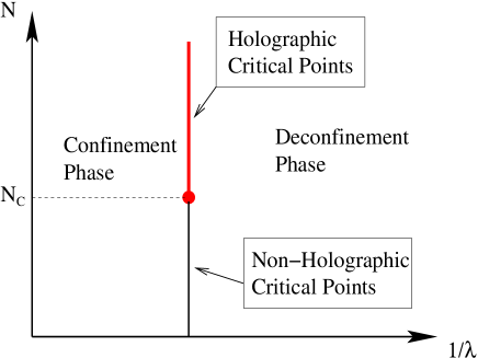
Figure 15: A proposed phase diagram for the pure bosonic gauged matrix model in $D>4$. Here $\lambda$ represents a set of ’t Hooft couplings associated with various Wilson loops in the matrix model. Moving along the direction of $\lambda$ in this figure may mean tuning more than one microscopic parameters at the same time. The critical points, in general, represent multi-critical points. Therefore the shape of the phase boundary in the figure should not be taken seriously. The actual phase boundary is not likely to be a straight line in the multi-dimensional space of microscopic couplings. In the strong coupling limit (large $\lambda$), the theory is in the confinement phase with the exponentially decaying Wilson loop correlation function. As the coupling becomes smaller, the model goes through a phase transition to the IR free deconfinement phase. For small $N$, $NS_{D-4}$-branes remain condensed at the critical point. Strings are confined, and the two-form gauge field is massive in the bulk. Critical correlations are mediated by the $D$-dimensional fluctuations of strings near the UV boundary. Scaling dimensions generally receive a large quantum correction at strong couplings. This is the non-holographic critical point. For large $N$, $NS_{D-4}$-brane is gapped and the two-form gauge field remains light even at strong coupling. Low energy physics is governed by deconfined strings that propagate deep inside the bulk. In this holographic critical point, critical correlations of the matrix model is mediated by $(D+1)$-dimensional fluctuations of strings. The scaling dimension of the operator associated with the two-form gauge field is protected from acquiring a large quantum correction due to the quantum order associated with the dynamical suppression of $NS_{D-4}$-branes. The holographic critical point can be either in the state with only closed strings, or in the state with both closed and open strings.

It may be difficult to find a specific microscopic model which realizes each phase discussed in this paper. However, one may still guess a possible phase diagram. For $D\leq 4$, it is believed that the present matrix model is always in the confinement phase. In these low dimensional cases, one may have to introduce more degrees of freedom (fermions or fundamental matters) to stabilize critical phases. Here we focus on the pure bosonic matrix model in $D>4$. In Fig. 15, we show a speculative phase diagram. In the strong coupling limit, the matrix model is in the confinement phase. As the gauge coupling is weakened, there is a phase transition into the IR free deconfinement phase. If the phase transition is continuous, there can be two different universality classes for the critical points. For small $N$, $NS_{D-4}$-branes are condensed and strings are confined in the bulk. At this non-holographic critical point, the scaling dimension of Wilson loop operators generally receive a large quantum correction. For $N$ greater than a critical value, $NS_{D-4}$-branes are suppressed, and strings are deconfined in the bulk. The quantum order protects the two-form gauge field from acquiring a large mass in the large $N$ limit, which in turn protects the scaling dimension of the phase fluctuations of Wilson loop operators even at large ’t Hooft couplings.

As was discussed in Sec. VII. E, there exist two different kinds of holographic critical points. In the first case, there are only closed string excitations in the bulk. In the second case, there are both closed and open string excitations along with the emergent gauge field and the two-form gauge field. We expect that it is easier to stabilize the state with both closed and open strings for $N$’s that are large but not too large. In the large $N$ limit, closed strings are free, and there is no dynamical reason why they decay into open strings. For $N$ large enough to suppress $NS_{D-4}$-brane, but still small enough to support strong interactions between closed strings, closed strings may decay into open strings. We believe that further studies are needed to understand this phenomenon more systematically.

It is of note that the structure of the proposed phase diagram is reminiscent of known examples where systems flow into novel universality classes at interacting critical points. For example, in the two-dimensional $Z_{N}$ clock model with $N$ greater than a critical value, the critical point between the disordered phase and the ordered phase has an emergent $U(1)$ symmetryZN . More recently, it has been proposed that the critical point between an antiferromagnetic state and a valence bond state in 2+1 dimensions can possess a non-trivial quantum order which supports an emergent gauge boson and fractionalized excitationsSENTHIL04 .

VIII.2 World sheet description of deconfined string

In order to make a contact with the traditional first quantization formulation of string theory, it will be useful to have a world-sheet description of deconfined strings in the holographic phases. Here we focus on closed string. The generalization to open string is straightforward. Note that the hopping integral from loop $C_{1}$ to $C_{1}+C_{2}$ is determined by the loop field $\bar{\phi}_{C_{2}}=|\bar{\phi}_{C_{2}}|e^{ib_{C_{2}}}$ which is complex. The amplitude $|\bar{\phi}_{C_{2}}|$ determines the strength of the hopping, and defines the notion of ‘distance’ between the two loops. The distance between two loops, in turn, defines the metric of the space in which loops are defined. In this sense, condensates of loop fields determine the metric of the space in which closed loops propagate. The $U(1)$ phase $b_{C_{2}}$ corresponds to the background two-form field to which closed strings are electrically coupled.

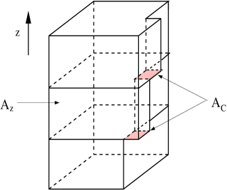
Figure 16: The world sheet action has two contributions : $A_{z}$ is the area of the surface which is parallel to $z$, and $A_{C}$ is the contribution from hoppings mediated by condensates of loop fields.

This can be made more intuitive if we use a world-sheet representation. Let us consider the the quadratic Hamiltonian that includes the tension and the hopping terms,

$$\displaystyle H_{0}(z) = L_{C}\chi_{C}^{\dagger}\chi_{C}-\frac{1}{M^{2}}\Bigl{(}2\bar{\phi}_{C_{2}}^{*}(z)\chi_{C_{1}}^{\dagger}\chi_{C_{1}+C_{2}}+2\bar{\phi}_{C_{2}}(z)\chi_{C_{1}+C_{2}}^{\dagger}\chi_{C_{1}}\Bigr{)}.$$ (81)

Here we suppressed the form factors $F_{ij}(C_{1},C_{2})$ and $G_{ij}(C_{1},C_{2})$. For this discussion, we ignore a possible deformation of the path integral of the string fields. We consider the single loop propagator given by

$$\displaystyle g(C_{2},z_{2};C_{1},z_{1}) = <C_{2}|e^{-\int_{z_{1}}^{z_{2}}H_{0}(z)dz}|C_{1}>,$$ (82)

where $|C>=\chi_{C}^{\dagger}|0>$ is a single string state. We can ‘re-discretize’ the imaginary time $z$ into small steps with size $\epsilon$ to write

$$\displaystyle g(C_{2},z_{2};C_{1},z_{1}) = \sum_{\mbox{all world sheets}}e^{-S_{WS}^{1}+iS_{WS}^{2}},$$ (83)

where

$$\displaystyle S_{WS}^{1}={\cal A}_{z}-\sum_{i}\ln(2\epsilon|\bar{\phi}_{C_{i}}(z_{i})|/M^{2}),$$ (84)

where ${\cal A}_{z}$ is the area of the world sheet whose faces are tangential to the $z$ direction, and the second term in $S_{WS}^{1}$ includes contributions $\frac{2\epsilon|\bar{\phi}_{C_{i}}(z_{i})|}{M^{2}}$ for each hopping mediated by loop field $\phi_{C_{i}}$ at time $z_{i}$. The second term is associated with the parts of the world sheet that are perpendicular to the $z$ direction. This is illustrated in Fig. 16. One can view $S_{SW}^{1}$ as the Nambu-Goto action provided that the area associated with a loop $C$ at time $z$ is taken to be $A_{C}=-\ln(2\epsilon|\bar{\phi}_{C}(z_{i})|/M^{2})$. The areas associated with loops in turn would determine the spatial metric of the space. The imaginary part of the action,

$$\displaystyle S_{WS}^{2}=\int_{\mbox{world sheet}}B$$ (85)

is simply the Berry phase associated with the phase of the background loop fields in the temporal gauge. Since both the phase and amplitude modes of loop fields are dynamical, not only the two-form gauge field but also a metric field should arise as a dynamical degree of freedom.

A typical configuration of vacuum fluctuation in the full interacting string theory are shown in Fig. 17. For every vertex where closed loops join or split, there is a factor of $1/N$. For a large $N$, the theory describes weakly interacting strings propagating in the time-dependent background.

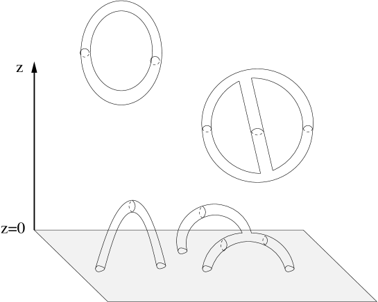
Figure 17: A snap shot of a vacuum fluctuation in the holographic critical phase with deconfined closed string.

VIII.3 Continuum limit

In the holographic phase, there are three important length scales. The first scale is associated with the tension $\mu_{NS_{D-4}}$ of $NS_{D-4}$-brane, $l_{NS_{D-4}}\sim 1/(\mu_{NS_{D-4}})^{D-3}$. The second scale is the ‘string scale’ $l_{s}$ which corresponds to the typical size of closed string excitation in the bulk. The third scale $L$ is the scale over which loop fields change appreciably in the bulk. Roughly, the last one determines the ‘curvature’ of the bulk space in which strings propagate. One can take the continuum limit by tuning the system such that all these length scales are fixed in the $a\rightarrow 0$ limit. If these scales satisfy $L>>l_{s}>>l_{NS_{D-4}}$, strings propagate in a weakly curved background. It is expected that a continuum description of string theory emerges in this limit. Since graviton has the same mass as the two-form gauge field in the continuum limit, graviton may emerge as a massless mode along with the two-form gauge field in the holographic phase. It will be interesting to see how the resulting theory in the continuum limit compares with the existing formulation of the closed string field theoryZWIEBACH .

IX Acknowledgment

I would like to thank G. Baskaran, Umut Gursoy, Sean Hartnoll, Ellias Kiritsis, Hong Liu, John McGreevy, Rob Myers and Subir Sachdev for helpful comments and discussions. This research was supported in part by the Natural Sciences and Engineering Research Council of Canada and the Early Research Award from the Ontario Ministry of Research and Innovation. Research at the Perimeter Institute is supported in part by the Government of Canada through Industry Canada, and by the Province of Ontario through the Ministry of Research and Information.

X Appendix A

We prove the identity

$$\displaystyle I = \int d\phi^{*}d\phi~{}~{}e^{-\phi(\phi^{*}-A^{*})}f(\phi^{*})$$ (86)

$$= \pi f(A^{*})$$

for any analytic function $f(x)$. We define a new variable $\xi=\phi-A$ to write

$$\displaystyle I = \int d\xi^{*}d\xi~{}~{}e^{-|\xi|^{2}-A\xi^{*}}f(\xi^{*}+A^{*})$$ (87)

$$= \sum_{m=0}^{\infty}\sum_{n=0}^{\infty}\frac{1}{m!n!}\int d\xi^{*}d\xi~{}~{}e^{-|\xi|^{2}}(-A\xi^{*})^{m}f^{(n)}(A^{*})\xi^{*n},$$

where we Taylor expanded $e^{A\xi^{*}}$ and $f(\xi^{*}+A^{*})$. Here only $m=n=0$ component survives in the angular integration of $\xi=|\xi|e^{i\theta}$ and we have

$$\displaystyle I = \pi f(A^{*}).$$ (88)

XI Appendix B

Here we show that Eq. (39) with Eqs. (40) - (43) is equivalent to Eq. (34). The imaginary time $\beta$ is divided into $R$ pieces,

$$\displaystyle Z = \int\prod_{l=1}^{R-1}d\Phi_{C}^{(l)*}d\Phi_{C}^{(l)}~{}<\Psi_{f}|e^{-\epsilon H}|\Phi_{C}^{(R-1)}>e^{-\Phi_{C}^{(R-1)*}\Phi_{C}^{(R-1)}}<\Phi_{C}^{(R-1)}|e^{-\epsilon H}|\Phi_{C}^{(R-2)}>\times$$ (89)

$$e^{-\Phi_{C}^{(R-2)*}\Phi_{C}^{(R-2)}}...<\Phi_{C}^{(2)}|e^{-\epsilon H}|\Phi_{C}^{(1)}>e^{-\Phi_{C}^{(1)*}\Phi_{C}^{(1)}}<\Phi_{C}^{(1)}|e^{-\epsilon H}|\Psi_{i}>,$$

where we use the identity

$$\displaystyle\int d\Phi_{C}^{(l)*}d\Phi_{C}^{(l)}~{}~{}|\Phi_{C}^{(l)}>e^{-\Phi_{C}^{(l)*}\Phi_{C}^{(l)}}<\Phi_{C}^{(l)}|=1.$$ (90)

For (40) and (42), the transition amplitude becomes

$$\displaystyle Z = \int\prod_{l=0}^{R}d\Phi_{C}^{(l)*}d\Phi_{C}^{(l)}~{}~{}\Psi_{f}^{*}[\Phi_{C}^{(R)*},\Phi_{C}^{(R)}]\Psi_{i}[\Phi_{C}^{(0)*},\Phi_{C}^{(0)}]~{}~{}e^{-S},$$ (91)

where

$$\displaystyle S = -\Phi_{C}^{(R)*}\Phi_{C}^{(R)}+\sum_{l=1}^{R}\left[\Phi_{C}^{(l)*}(\Phi_{C}^{(l)}-\Phi_{C}^{(l-1)})+\epsilon H(\Phi_{C}^{(l)*},\Phi_{C}^{(l-1)})\right].$$ (92)

We take $R\rightarrow\infty$ limit and equate Eq. (92) with Eq. (34) to identify

$$\displaystyle\Psi_{i}[\Phi_{C}^{*},\Phi_{C}] = e^{-S_{UV}[\Phi_{C}^{*}/N,\Phi_{C}/N]},$$

$$\Psi_{f}^{*}[\Phi_{C}^{*},\Phi_{C}] = e^{-\Phi_{C}^{*}\Phi_{C}-S_{IR}[\Phi_{C}/N]}.$$ (93)

XII Appendix C

Figure 18:

In this section, we solve the loop equations perturbative in $1/M$ to the lowest non-trivial order for small loops. Let us first consider the saddle point solution in the large $M$ limit, which corresponds to the deep inside the confinement phase of the gauge theory. For $M=\infty$, we have simple solution,

$$\displaystyle\phi_{C}(z)=\phi_{C}(0)e^{-L_{C}z},~{}~{}~{}\phi_{C}^{*}(z)=\phi_{C}^{*}(0)e^{L_{C}z}$$ (94)

with the boundary conditions in Eqs. (65) and (66). Especially, the IR boundary condition implies $\phi_{C}^{*}(\infty)=0$, which then implies $\phi_{C}^{*}(z)=0$. This makes sense physically because the source for Wilson loops decreases exponentially with $z$, and the expectation values of Wilson loop operators vanish in the strong coupling limit of the gauge theory. For a large but finite $M$, the loop equations can be solved perturbatively in $1/M$.

To illustrate the idea, we solve the loop equation for a simple model which include only the single trace operator for the unit plaquette, $V=J_{\Box}\phi_{\Box}^{*}$. In this model, we solve $\phi_{\Box}^{*}$ to the lowest order in $1/M$. Keeping the first four shortest loops that contribute to the evolution of $\phi_{C}^{*}$ of unit plaquette, we write the saddle point equations,

$$\displaystyle\partial_{z}\phi_{\Box}^{*} = 4\phi_{\Box}^{*}-\frac{2}{M^{2}}(\phi_{\sqcup}^{*}+\phi_{\sqcap}^{*}+\phi_{\sqsubset}^{*}+\phi_{\sqsupset}^{*})\phi_{\bar{\Box}},$$

$$\partial_{z}\phi_{\sqcup}^{*} = 6\phi_{\sqcup}^{*}-\frac{2}{M^{2}}(\phi_{\lfloor}^{*}+\phi_{\mid}^{*2}+\phi_{\rfloor}^{*}),$$

$$\partial_{z}\phi_{\lfloor}^{*} = 4\phi_{\lfloor}^{*}-\frac{2}{M^{2}}(\phi_{\mid}^{*}+\phi_{-}^{*}),$$

$$\partial_{z}\phi_{-}^{*} = 2\phi_{\Box}^{*}-\frac{2}{M^{2}}.$$ (95)

The symbols are defined in Fig. 18. We consider solutions with the translational and discrete rotational symmetries of the lattice, and suppress the site index for the loop fields. The equations for $\phi_{\sqcap}^{*}$, $\phi_{\sqsubset}^{*}$ and $\phi_{\sqsupset}$ are similar to the one for $\phi_{\sqcup}^{*}$. Similarly, the equation for $\phi_{\rfloor}^{*}$ ($\phi_{\mid}$) is similar to the one for $\phi_{\lfloor}^{*}$ ($\phi_{-}$). From Eqs. (32) and (66), we read the boundary conditions,

$$\displaystyle\phi_{\Box}^{*}(\infty)=\frac{\phi_{\bar{\Box}}(\infty)}{M^{8}},~{}~{}~{}\phi_{\sqcup}^{*}(\infty)=\frac{1}{M^{6}},$$

$$\phi_{\lfloor}^{*}(\infty)=\frac{1}{M^{4}},~{}~{}~{}\phi_{-}^{*}(\infty)=\frac{1}{M^{2}}.$$ (96)

Using the zero-th order solution for $\phi_{\bar{\Box}}=J_{\bar{\Box}}e^{-4z}$, we obtain

$$\displaystyle\phi_{\Box}^{*}(z)=\frac{J_{\bar{\Box}}}{M^{8}}e^{-4z}.$$ (97)

This implies that the expectation value of the Wilson loop operator for the unit plaquette become $J_{\bar{\Box}}/M^{8}$ as expected in the large $M$ limit. The difference from the case with $M=\infty$ is that $\phi_{C}^{*}$ is now non-zero at $z=0$ because Wilson loops have non-zero expectation values. As expected, $\phi_{C}$ and $\phi_{C}^{*}$ satisfy Eq. (67) to the leading order in $1/M$ at all $z$.

References

- (1) P. W. Anderson, Science 235 (1987) 1196 ; P. Fazekas and P. W. Anderson, Philos. Mag. 30 (1974) 432.
- (2) G. Baskaran, Z. Zou and P. W. Anderson, Solid State Commun. 63 (1987) 973; G. Baskaran and P. W. Anderson, Phys. Rev. B 37 (1988) 580.
- (3) For more comprehensive reviews on the application of slave-particle theory to condensed matter systems, see P. A. Lee, N. Nagaosa and X.-G. Wen, Rev. Mod. Phys. 78 (2006) 17; S. Sachdev, arXiv:0901.4103; L. Balents, Nature 464 (2010) 199.
- (4) X.-G. Wen, Phys. Rev. B 65 (2002) 165113.
- (5) J. M. Maldacena, Adv. Theor. Math. Phys. 2 (1998) 231.
- (6) S. S. Gubser, I. R. Klebanov and A. M. Polyakov, Phys. Lett. B 428 (1998) 105.
- (7) E. Witten, Adv. Theor. Math. Phys. 2 (1998) 253.
- (8) A. Polyakov Nucl. Phys. B 164 (1980) 171.
- (9) B. Sakita, Phys. Rev. D 21 (1980) 1067.
- (10) Y. Makeenko and A. Migdal, Nucl. Phys. B 188 (1981) 269.
- (11) A. Jevicki and B. Sakita, Nucl. Phys. B 185 (1981) 89.
- (12) S.-S. Lee, Nucl. Phys. B 832 (2010) 567.
- (13) S.-S. Lee, Nucl. Phys. B 851 (2011) 143.
- (14) E. T. Akhmedov, Phys. Lett. B 442 (1998) 152; E. T. Akhmedov, hep-th/0202055.
- (15) S. R. Das and A. Jevicki, Phys. Rev. D 68 (2003) 044011.
- (16) R. Gopakumar, Phys. Rev. D 70 (2004) 025009; ibid. 70 (2004) 025010.
- (17) I. Heemskerk, J. Penedones, J. Polchinski and J. Sully, J. High Energy Phys. 10 (2009) 079.
- (18) R. Koch, A. Jevicki, K. Jin and J. P. Rodrigues, arXiv:1008.0633.
- (19) M. Douglas, L. Mazzucato, and S. Razamat, Phys. Rev. D 83 (2011) 071701.
- (20) R. Sundrum. arXiv:1106.4501.
- (21) J. de Boer, E. Verlinde and H. Verlinde, J. High Energy Phys. 08 (2000) 003.
- (22) M. Li, Nucl. Phys. B 579 (2000) 525.
- (23) I. Heemskerk and J. Polchinski, arXiv:1010.1264.
- (24) T. Faulkner, H. Liu and M. Rangamani, arXiv:1010.4036.
- (25) S.-J. Sin and Y. Zhou, J. High Energy Phys. 1105 (2011) 030.
- (26) S.-S. Lee and P. A. Lee, Phys. Rev. B 72 (2005) 235104.
- (27) J. Polchinski, Nucl. Phys. B 231 (1984) 269.
- (28) J. Polonyi, arXiv:hep-th/0110026v2.
- (29) M. Kalb and P. Ramond, Phys. Rev. D 9 (1974) 2273.
- (30) N. Ishibashi and H. Kawai, Phys. Letts. B 314 (1993) 190; M. Ikehara, N. Ishibashi, H. Kawai, T. Mogami, R. Nakayama, and N. Sasakura, Phys. Rev. D 50 (1994) 7467; N. Ishibashi and H. Kawai, Phys. Letts. B 352 (1995) 75.
- (31) A. Jevicki and J. P. Rodrigues, Nucl. Phys. B 421 (1994) 278; R. Koch, A. Donos, A. Jevicki and J. P. Rodrigues, Phys. Rev. D 68 (2003) 065012; R. Koch, A. Jevicki and J. P. Rodrigues, Int. J. Mod. Phys. A 19 (2004) 1747.
- (32) J. Lykken and S. Raby, Nucl. Phys. B 278 (1986) 256.
- (33) G. T. Horowitz, J. Lykken, R. Rohm and A. Strominger, Phys. Rev. Lett. 57 (1986) 283.
- (34) E. Witten, hep-th/0112258.
- (35) C. G. Callan and S. Coleman, Phys. Rev. D 16 (1977) 1762.
- (36) H. Reinhardt, Nucl. Phys. A 367 (1981) 269.
- (37) A. M. Polyakov, Phys. Scr. T 15 (1987) 191.
- (38) S.-J. Rey, Phys. Rev. D 43 (1991) 526.
- (39) F. Quevedo and C. A. Trugenberger, Nucl.Phys. B 501 (1997) 143.
- (40) G. T. Horowitz and E. Silverstein, Phys. Rev. D 73 (2006) 064016.
- (41) P. Orland, Nucl.Phys. B205 (1982) 107.
- (42) R. B. Pearson, Phys. Rev. D 26 (1982) 2013.
- (43) S.-J. Rey, Phys. Rev. D 40 (1989) 3396.
- (44) O. Aharony and E. Witten, J. of High Ener. Phys. 11 (1998) 018.
- (45) J. Maldacena, N. Seiberg and G. Moore, J. of High Ener. Phys. 10 (2001) 005.
- (46) P. Yi, Nucl. Phys. B 550 (1999) 214.
- (47) S. R. Das and S. P. Trivedi, Phys.Lett. B 445 (1998) 142 (hep-th/9804149).
- (48) J. V. Jose, L. P. Kadanoff, S. Kirkpatrick and D. R. Nelson, Phys. Rev. B 16 (1977) 1217.
- (49) T. Senthil, A. Vishwanath, L. Balents, S. Sachdev and M. P. A. Fisher, Science 303 (2004) 1490.
- (50) B. Zwiebach, Nucl. Phys. B 390 (1993) 33.