Competitive Privacy in the Smart Grid: An Information-theoretic Approach

Abstract

Advances in sensing and communication capabilities as well as power industry deregulation are driving the need for distributed state estimation at the regional transmission organizations (RTOs). This leads to a new competitive privacy problem amongst the RTOs since there is a tension between sharing data to ensure network reliability (utility/benefit to all RTOs) and withholding data for profitability and privacy reasons. The resulting tradeoff between utility, quantified via fidelity of its state estimate at each RTO, and privacy, quantified via the leakage of the state of one RTO at other RTOs, is captured precisely using a lossy source coding problem formulation for a two RTO network. For a two-RTO model, it is shown that the set of all feasible utility-privacy pairs can be achieved via a single round of communication when each RTO communicates taking into account the correlation between the measured data at both RTOs. The lossy source coding problem and solution developed here is also of independent interest.

I Introduction

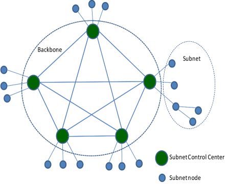
The electric power industry is undergoing profound changes as greater emphasis is placed on the importance of a smarter grid that supports sustainable energy utilization. Technically, enabled by advances in sensing, communication, and actuation, power system estimation and control are likely to involve many more fast information gathering and processing devices (e.g. Phasor Measurement Units) [1]. Economically, the deregulation of the electricity industry has led to the creation of many regional transmission organizations (RTOs) within a large interconnected power system [2] (see Fig. 1). Both technical and economic drivers suggest the need for more distributed estimation and control in power system operations.

Figure 1: Mutiple RTOs (subnets) connected via the transmission network.

Distributed Cooperation: While the distributed state estimation problem has been investigated for well over two decades, the focus to date has been on two-tier hierarchical models [3] in which each local control center (e.g., RTO) estimates independently without sharing any information amongst its neighbors, and at a higher level, a central coordinator receives the estimation results from the individual areas and coordinates them to obtain a system-wide solution. However, such an hierarchical approach does not scale with increasing measurement rates due to communication and reliability challenges inherent in systems with one coordination center. Furthermore, the interconnectedness of the RTOs makes the problem of wide area monitoring and control (e.g. for the entire Eastern United States interconnection) important and immediate. This requirement of sharing the entire system state amongst all the RTOs is driving the need for a fully distributed approach to state estimation wherein the local control centers interactively estimate the system state as a whole.

There are several challenges that arise in the context of a fully distributed state estimation approach. We address a specific problem of collaboration and competition by introducing a framework that precisely quantifies the tradeoff between the utility (benefit) of collaboration and the resulting privacy leakage.

Competitive Privacy: The problem of end-user privacy has begun receiving attention with the deployment of smart meters to monitor and finely manage user power consumption [4, 5, 6, 7, 8, 9]. In contrast, a new competitive privacy problem arises at the level of the RTOs due to the conflict between sharing data for distributed estimation and withholding data for economic (competitive) and end-user privacy reasons, i.e., there is a tradeoff between sharing data to ensure network reliability (utility/benefit to all RTOs) and withholding data to ensure profitability and privacy.

Competitive privacy has been studied by the database community in the context of data integration from multiple autonomous sources that do not wish to reveal private sensitive business information to one another and yet benefit from the combined analysis [10]. However, the solutions proposed are unique for databases and do not directly apply to the distributed state estimation problem discussed above. An analytical framework that abstracts the problem of competitive privacy via appropriate source models and utility and privacy metrics is required and it is this problem that we address in this paper.

Utility vs. Privacy: Utility and privacy are competing goals: utility is maximized when the RTOs completely disclose their measurements to each other; however, privacy is minimal for this disclosure. On the other hand, not sharing any data guarantees maximal privacy but achieves zero utility. Thus, ensuring privacy requires distorting or perturbing the data which also provide utility guarantees. The theory of rate distortion allows us to study this tradeoff between privacy and utility using appropriate metrics for both constraints; we present such a formal framework in this paper for the competitive privacy problem.

Contributions: In this paper, we present a linear measurement model for the grid at the level of the RTOs that takes into account the interconnections amongst them. Viewing the power system state at each RTO as an information source, we model the measurements at each RTO as a linear combination of all the sources. The competitive privacy problem formulated thus leads to a new distributed lossy source coding problem wherein each RTO shares (encodes) a perturbed function of its measurements, and over a finite number of such communication rounds, estimates its state subject to two constraints: a) each RTO must be able to decode its own measurements to a desired fidelity, and b) at each RTO, the privacy leakage of the measurements shared by the other RTOs must be bounded.

Distributed source coding has received much attention recently with a growing interest in sensor networks. However, with a few exceptions, most distributed source coding problems remain open. One such exception is the quadratic Gaussian CEO problem in which a source is observed noisily by multiple sensors, each of which uses a finite-rate link to communicate it to a single receiver which in turn combines these messages to reconstruct the source to a desired level of fidelity [11]. The problem presented here further generalizes such a setting in the following ways: a) there are multiple sources, b) each sensor (here RTO) is now both an encoder and a decoder, i.e., there are multiple encoders and decoders, and c) there are fidelity requirements at each RTO for its own measurements and privacy requirements vis-à-vis other measurements.

Having modeled the general problem, we focus on a two-source setting that captures the distributed estimation problem for two large RTOs. Using distortion as a metric for utility and mutual information as a metric for privacy leakage, we demonstrate that a single-shot rate-distortion code at each RTO that is cognizant of the side information (measurement vector) at the other RTO achieves the set of all feasible utility-privacy operating points.

The paper is organized as follows: in Section II, we develop the model and present abstract metrics for utility and privacy. In Section III, we present our main results. We conclude in Section IV.

II Model and Metrics

II-A Model

Let $M$ denote the total number of RTOs and let $X_{m}$ denote the power system state variable at the $m^{th}$ RTO, $m=1,2,\ldots,M$. Assuming linearized system dynamics, the general measurement model at the $k^{th}$ terminal at a sampling time instant is given by

$$Y_{m}={\textstyle\sum\limits_{j=1}^{M}}H_{m,j}X_{j}+Z_{m},\text{ }m=1,2,\ldots,M,$$ (1)

where $X_{m}\sim\mathcal{N}\left(0,1\right)$, for all $m,$ are assumed to be mutually independent, and where $H_{m,j}$ denotes the Jacobian modeling the linearized dynamics between the $j^{th}$ state and the measurement at the $m^{th}$ RTO. The observation noise at the $m^{th}$ RTO $Z_{m}\sim\mathcal{N}\left(0,\sigma_{m}^{2}\right)$ is assumed to be independent of $X_{m}$, for all $m$. We assume that the $H_{m,j}$ are fixed and known at all RTOs for the duration of communications; furthermore, we also assume that the statistics of the noise, the measurements, and the states are known at all the RTOs. In this paper, we focus on case of $M=2$, i.e., we are interested in the distributed estimation problem between two (typically large) adjacent RTOs. Finally, we set $H_{1,1}=H_{2,2}=1$, $H_{1,2}=\alpha\in\left(0,\infty\right)$, and $H_{2,1}=\beta\in\left(0,\infty\right)$.

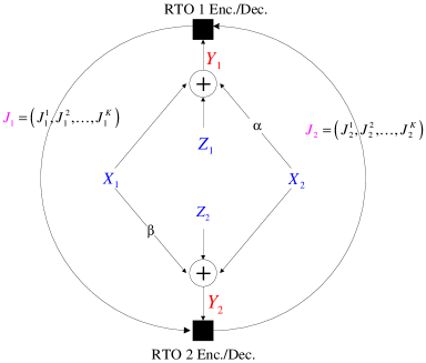
We assume that the $m^{th}$ RTO observes a sequence of $n$ measurements $Y_{m}^{n}=[Y_{m,1}$ $Y_{m,2}$ $\ldots$ $Y_{m,n}]$, for all $m$, over a window of time prior to communications. The communication protocol is shown in Fig. 2 for $M=2$. In each communication round, the two RTOs take turns such that each RTO encodes (quantizes) its measurements taking into account the fact the other RTO has correlated side information (the correlations come from the measurement vectors at each RTO being functions of the state variables at both RTOs). We assume a total of $K$ such communication rounds before RTO $m$ estimates $\hat{X}_{m}^{n}$, $m=1,2$, using the entire sequence of public communications and its own measurements.

Figure 2: Communication protocol for two RTOs.

II-B Metrics

Utility: The motivation for cooperation at each RTO is to obtain a good estimate of its own system state. Thus, for our continuous Gaussian distributed state model, a reasonable metric for utility at the $m^{th}$ RTO is the mean square error $D_{m}$ of the original and the estimated state sequences $X_{m}^{n}$ and $\hat{X}_{m}^{n}$, respectively.

Privacy: The measurements at each RTO in conjunction with the quantized data from the other RTO while enabling estimation of its own state can also potentially leak information about the state at the other RTO. We capture this information leakage via the mutual information.

II-C Communication Protocol

A coding scheme for the network involves an encoder-decoder pair at each RTO over $K$ communication rounds such that some desired utility and privacy values are achieved. Formally, an $(n,K,M_{1},M_{2},D_{1},D_{2},L_{1},L_{2})$ code for this network results from a $K$-round protocol in which RTO $m$, $=1,2,$ uses the encoding functions $\left\{f_{m,k}\right\}$ for the $k^{th}$ round and a decoding function $F_{m}$ at the end of the $K$ rounds. In round $k$, the encoder at RTO $m$ maps its measurements and the messages received until then from the other RTO to an index set $\mathcal{J}_{m}^{k}$ where

$$\mathcal{J}_{m}^{k}\equiv\left\{1,2,\ldots,J_{m}^{k}\right\}\text{, }k=1,2,\ldots K,\text{ }m=1,2,$$ (2)

is the index set at the $m^{th}$ RTO for mapping the quantized sequence in the $k^{th}$ protocol round via the encoder $f_{m}^{k}$ defined as

$$f_{m}^{k}:\mathcal{Y}_{m}^{n}\times\mathcal{J}_{m}^{1}\times\ldots\times\mathcal{J}_{m}^{k-1}\rightarrow\mathcal{J}_{m}^{k},\text{ }k=1,2,\ldots K,m=1,2,$$ (3)

such that at the end of the $K$ rounds, the decoding function $F_{m}$ at the $m^{th}$ RTO is a mapping from the space of measurements and received messages to that of the reconstructed sequence denoted as

$$F_{m}:\mathcal{Y}_{m}^{n}\times\mathcal{J}_{m}^{1}\times\ldots\times\mathcal{J}_{m}^{K}\rightarrow\mathcal{\hat{X}}_{m}^{n},\text{ \ }m=1,2.$$ (4)

Let $J_{m}\equiv\left\{J_{m}^{k}\right\}_{k=1}^{M}$, denote the set of all indices communicated by the $m^{th}$ RTO, $m=1,2$, such that $M_{1}$ and $M_{2}$ denote the size of $J_{1}$ and $J_{2}$, respectively. The expected distortion $D\,_{m}\$at the $m^{th}$ RTO is given by

$$D_{m}=\frac{1}{n}\mathbb{E}\left[{\textstyle\sum\limits_{i=1}^{n}}\left(X_{m,i}-\hat{X}_{m,i}\right)^{2}\right]\text{, }m=1,2,$$ (5)

and the privacy leakage, $L_{1}$, about state $1$ at RTO $2$ is given by

$$L_{1}=\frac{1}{n}I\left(X_{1}^{n};J_{1},J_{2},Y_{2}^{n}\right),$$ (6)

and the privacy leakage, $L_{2}$, about state $2$ at RTO $1$ is given by

$$L_{2}=\frac{1}{n}I\left(X_{2}^{n};J_{1},J_{2},Y_{1}^{n}\right).$$ (7)

The communication rate of the $m^{th}$ RTO is denoted by

$$R_{m}=n^{-1}\log_{2}M_{m},m=1,2.$$ (8)

Definition 1

The utility-privacy tradeoff region $\mathcal{T}$ is the set of all $\left(D_{1},D_{2},L_{1},L_{2}\right)$ for which there exists a coding scheme given by (2)-(4) with parameters $(n,K,M_{1},M_{2},D_{1}+\epsilon,D_{2}+\epsilon,L_{1}+\epsilon,L_{2}+\epsilon)$ for $n$ sufficiently large such that $\epsilon\rightarrow 0$ as $n\rightarrow\infty$.

III Main Results

The coding and communication protocol described in the previous section is constrained only by the fidelity requirements of the desired state estimate at each RTO and the privacy leakage of the state at the other RTO. Furthermore, from Definition 1, we note that the utility-privacy tradeoff region $\mathcal{T}$ is also dependent on size of the encoding indices $M_{1}$ and $M_{2}\,,$ i.e., for every $\left(D_{1},D_{2},L_{1},L_{2}\right)\in\mathcal{T}$, there can be several achievable coding schemes each corresponding to some communication rate pair $\left(R_{1},R_{2}\right)$. Thus, it suffices to determine the set of all rate-distortion-leakage $\left(R_{1},R_{2},D_{1},D_{2},L_{1},L_{2}\right)$ tuples to determine the utility-privacy tradeoff region.

III-A Rate-Distortion-Leakage (RDL) Tradeoff

Recall that $Y_{1}=X_{1}+\alpha X_{2}+N_{1}$ and $Y_{2}=\beta X_{1}+X_{2}+N_{2}$, where $X_{m}\sim\mathcal{N}(0,1),m=1,2$, and $N_{m}\sim\mathcal{N}(0,\sigma_{m}^{2}),m=1,2$, are all mutually independent. We first state the range of allowable distortion pairs $\left(D_{1},D_{2}\right)$ as

$$D_{m}\in[D_{\min,m},D_{\max,m}],m=1,2,$$

where

$$D_{\min,1} =1-\frac{(\beta^{2}V_{1}+V_{2}-2\beta E)}{(V_{1}V_{2}-E^{2})}$$ (9a)

$$D_{\min,2} =1-\frac{(V_{1}+\alpha^{2}V_{2}-2\alpha E)}{(V_{1}V_{2}-E^{2})},$$ (9b)

and

$$D_{\max,1}=1-\frac{1}{V_{1}},\quad D_{\max,2}=1-\frac{1}{V_{2}},$$ (10a)

for

$$V_{1} \equiv 1+\alpha^{2}+\sigma_{1}^{2},$$ (11a)

$$V_{2} \equiv 1+\beta^{2}+\sigma_{2}^{2}\text{, and}$$ (11b)

$$E \equiv\alpha+\beta.$$ (11c)

The lower bounds $$D_{\min,1} D_{\min,2} D_{1} D_{2} (Y_{1},Y_{2}) X_{1} X_{2} D_{\min,1} D_{\min,2}$$ and on and in (9), respectively, are obtained by considering an enhanced system, in which both observations can be jointly used for estimating and . For such a system, the minimum mean square error (MMSE) estimator minimizes the quadratic distortion in (5). Therefore, and are given by

$$D_{\min,1} =\mathbb{E}\left[var(X_{1}|Y_{1},Y_{2})\right]$$ (12)

$$D_{\min,2} =\mathbb{E}\left[var(X_{2}|Y_{1},Y_{2})\right]$$ (13)

where for two random variables $A$ and $B$, $var\left(A|B\right)$ is the conditional variance of $A$ conditioned on $B.$ On the other hand, $D_{\max,1}$ and $D_{\max,2}$ correspond to the fidelity criterion achievable using only the locally available measurements at each RTO such that

$$D_{\max,1} =\mathbb{E}\left[var(X_{1}|Y_{1})\right]$$ (14)

$$D_{\max,2} =\mathbb{E}\left[var(X_{2}|Y_{2})\right].$$ (15)

The range of feasible leakage values $L_{1}$ and $L_{2}$ are

$$L_{1} \in[I(X_{1};Y_{2}),I(X_{1};Y_{1},Y_{2})],\text{ and}$$ (16)

$$L_{2} \in[I(X_{2};Y_{1}),I(X_{2};Y_{1},Y_{2})].$$ (17)

The lower bound on $L_{1}$, i.e., $I(X_{1};Y_{2})$ is guaranteed only for the case in which there is no public communication. This scenario can arise if $D_{1}$ and $D_{2}$ can be achieved at each RTO with its own measurements (corresponding to $D_{\max,1}$ and $D_{\max,2}$, respectively). At the other extreme, the maximum value of leakage $L_{1}$ can go up to $I(X_{1};Y_{1},Y_{2})$. This corresponds to an infinite rate transmission from RTO $1$ to RTO $2$ to satisfy the distortion requirement $D_{2}=D_{\min,2}$. A similar upper bounding argument holds for $L_{2}$.

Finally, we exploit the Gaussian nature of the system variables to write

$$E[X_{1}|Y_{1},Y_{2}] =k_{1}Y_{1}+k_{2}Y_{2}$$ (18a)

$$E[X_{2}|Y_{1},Y_{2}] =l_{1}Y_{1}+l_{2}Y_{2}$$ (18b)

where

$$k_{1} =\frac{V_{2}-\beta E}{V_{1}V_{2}-E^{2}},\quad k_{2}=\frac{\beta V_{1}-E}{V_{1}V_{2}-E^{2}},\hbox{ and}$$ (19a)

$$l_{1} =\frac{\alpha V_{2}-E}{V_{1}V_{2}-E^{2}},\quad l_{2}=\frac{V_{1}-\alpha E}{V_{1}V_{2}-E^{2}}.$$ (19b)

Using these results, we now summarize the rate-distortion-leakage tradeoff for the problem under consideration in the following theorem.

Theorem 2

The rate-distortion-leakage tradeoff $\left(R_{1},R_{2},D_{1},D_{2},L_{1},L_{2}\right)$ is given as follows.

If $D_{2}\in[D_{\min,2},D_{\max,2}]$, then

$$R_{1} =\frac{1}{2}\log\left(\frac{(V_{1}V_{2}-E^{2})l_{1}^{2}}{V_{2}(D_{2}-D_{\min,2})}\right),\text{ and}$$ (20)

$$L_{1} =\frac{1}{2}\log\left(\frac{l_{1}^{2}}{l_{1}^{2}D_{\min,1}+k_{1}^{2}(D_{2}-D_{\min,2})}\right).$$ (21)

If $D_{2}\geq D_{\max,2}$, then

$$R_{1} =0,\text{ and}$$ (22)

$$L_{1} =\frac{1}{2}\log\left(V_{2}\left/\left(V_{2}-\beta\right)\right.\right).$$ (23)

If $D_{1}\in[D_{\min,1},D_{\max,1}]$,

$$R_{2} =\frac{1}{2}\log\left(\frac{(V_{1}V_{2}-E^{2})k_{2}^{2}}{V_{1}(D_{1}-D_{\min,1})}\right),\text{ and}$$ (24)

$$L_{2} =\frac{1}{2}\log\left(\frac{k_{2}^{2}}{k_{2}^{2}D_{\min,2}+l_{2}^{2}(D_{1}-D_{\min,1})}\right).$$ (25)

If $D_{1}\geq D_{\max,1}$, then

$$R_{2} =0,\text{ and}$$ (26)

$$L_{2} =\frac{1}{2}\log\left(V_{1}\left/\left(V_{1}-\alpha\right)\right.\right),$$ (27)

where $D_{\min,m},$ $D_{\max,m}$, $V_{m}$, $E,$ and $l_{m}$, $k_{m}$, $m=1,2,$ are defined in (9), (10a), (11), and (19).

Remark 3

Theorem 2 shows that the optimal rate-distortion-leakage tradeoff for the Gaussian case admits a decoupling with respect to the distortion pair $(D_{1},D_{2})$. By decoupling, we mean that the leakage of source $X_{1}$ and the transmission rate of RTO $1$ depends solely on the distortion $D_{2}$ desired by RTO $2$. Similarly, the leakage of $X_{2}$ and the transmission rate of RTO $2$ depends solely on the distortion $D_{1}$ desired by RTO $1$. The reason for this decoupling can be attributed to the no rate-loss property of jointly Gaussian sources, which can be described as follows: if RTO $2$ is interested in reconstructing $X_{2}$ at a distortion $D_{2}$, then the minimal rate of transmission required by RTO $1$ remains unchanged even if the source $Y_{2}$ is available at RTO $1$.

We briefly sketch the proof below; we first derive lower bounds on the rate and privacy leakage and present a coding scheme that achieves them.

Proof:

Lower bound on $R_{1},R_{2}:$ Recall that we write $J_{1}$ to denote the message from RTO 1 over all $K$ communication rounds. Given a distortion pair $(D_{1},D_{2})$, we prove the lower bound on $R_{1}$ as follows:

$$nR_{1} =H(J_{1})$$ (28a)

$$\geq I(Y_{1}^{n};J_{1}|Y_{2}^{n})$$ (28b)

$$\geq nh(Y_{1}|Y_{2})-\sum_{t=1}^{n}h(Y_{1t}|J_{1},Y_{2}^{n})$$ (28c)

$$\geq nh(Y_{1}|Y_{2})-\sum_{t=1}^{n}\frac{1}{2}\log\left(2\pi e\mbox{Var}(Y_{1t}|J_{1},Y_{2}^{n})\right)$$ (28d)

$$\geq nh(Y_{1}|Y_{2})-\frac{n}{2}\log\left(2\pi e\sum_{t=1}^{n}\mbox{Var}(Y_{1t}|J_{1},Y_{2}^{n})/n\right)$$ (28e)

$$\geq nh(Y_{1}|Y_{2})-\frac{n}{2}\log\left(2\pi e(D_{2}-D_{\min,2})/l_{1}^{2}\right)$$ (28f)

$$=\frac{n}{2}\log(2\pi e(V_{1}V_{2}-E^{2})/V_{2})$$

$$\quad-\frac{n}{2}\log\left(2\pi e(D_{2}-D_{\min,2})/l_{1}^{2}\right)$$ (28g)

$$=\frac{n}{2}\log\left(\frac{(V_{1}V_{2}-E^{2})l_{1}^{2}}{V_{2}(D_{2}-D_{\min,2})}\right)$$ (28h)

where the inequalities in (28) follow from the chain rule, the fact that conditioning does not increase entropy, the fact that Gaussian distribution maximizes the differential entropy for a given variance, and the concavity of the $$\log Y_{1t} J_{1} Y_{2}^{n} R_{2} R_{1} R_{2}$$ function. The variance of conditioned on and can be computed using (18) and (19) and is omitted due to space limitations. A lower bound on can be obtained similarly. Therefore, and can be lower bounded by the expressions in (20) and (24), respectively.

Lower bounds on $\left(L_{1},L_{2}\right):$ Given an arbitrary code that achieves a certain distortion pair $(D_{1},D_{2})$, we derive lower bound on the leakages for both RTOs as follows:

$$L_{1} \geq\frac{1}{n}I(X_{1}^{n};J_{1},J_{2},Y_{2}^{n})$$ (29a)

$$\geq h(X_{1})-\frac{1}{n}h(X_{1}^{n}|J_{1},J_{2},Y_{2}^{n})$$ (29b)

$$\geq h(X_{1})-\frac{1}{n}h(X_{1}^{n}|J_{1},Y_{2}^{n})$$ (29c)

$$\geq h(X_{1})-\frac{1}{n}h(X_{1}^{n}|J_{1},Y_{2}^{n})$$ (29d)

$$\geq h(X_{1})-\frac{1}{n}\sum_{t=1}^{n}h(X_{1t}|J_{1},Y_{2}^{n})$$ (29e)

$$\geq h(X_{1})-\frac{1}{n}\sum_{t=1}^{n}\frac{1}{2}\log(2\pi e\mbox{ Var}(X_{1t}|J_{1},Y_{2}^{n}))$$ (29f)

$$\geq h(X_{1})-\frac{1}{2}\log\left(2\pi e\frac{1}{n}\sum_{t=1}^{n}\mbox{ Var}(X_{1t}|J_{1},Y_{2}^{n})\right)$$ (29g)

$$\geq h(X_{1})-\frac{1}{2}\log\left(2\pi e(D_{\min,1}+k_{1}^{2}(D_{2}-D_{\min,2})/l_{1}^{2})\right)$$ (29h)

where the inequalities in (29) follow from the chain rule, the fact that conditioning does not increase entropy, the fact that Gaussian distribution maximizes the differential entropy for a given variance, and the concavity of the $$\log L_{2} L_{1} L_{2}$$ function. A lower bound on can be obtained similarly. Simplifying further, we can lower bound and with the expressions in (21) and (25), respectively.

Upper bounds on $\left(R\,_{1},R_{2}\right)$ and $\left(L_{1},L_{2}\right)$ via an achievable coding scheme: The lower bounds derived above can be achieved using the Wyner-Ziv source coding scheme with decoder side information [12] at each RTO. We briefly describe the encoding scheme at RTO 1 and the resulting decoding at RTO 2; the coding scheme for RTO 2 follows analogously. The encoding is such that RTO $1$ generates a set of $M_{1}$ sequences $U_{1}^{n}\left(j_{1}\right)$, $j_{1}=1,2,\ldots,M_{1}$, where $M_{1}=2^{n\left(I(U_{1};Y_{1})+\epsilon\right)}$. However, to exploit the fact that RTO 2 has correlated measurements, RTO $1$ further bins its $M_{1}$ sequences into $S_{1}$ bins chosen at random where $S_{1}=2^{n\left(I(U_{1};Y_{1})-I(U_{1};Y_{2})+\epsilon\right)}$. Upon observing a measurement sequence $y_{1}^{n},$ the encoder at RTO 1 searches for a $U_{1}^{n}\left(j_{1}\right)$ sequence such that $y_{1}^{n}$ and $u_{1}^{n}\left(j_{1}\right)$ are jointly typical (as defined in [13, Chap. 10]) where the choice of $M_{1}$ ensures that there exists at least one such $j_{1}$. Using the fact that RTO 2 has its own measurements $Y_{2}^{n}$ as side information, the encoder at RTO 1 sends only $b\left(j_{1}\right)$ where $b\left(j_{1}\right)$ is the bin index of the $u_{1}^{n}\left(j_{1}\right)$ sequence.

For Gaussian distributed state and measurements, the sequence $U_{1}^{n}$ is chosen such that the ‘test channel’ from $U_{1}$ to $Y_{1}$ yields $Y_{1}=U_{1}+Q_{1}$, where $Q_{1}$ is a Gaussian random variable, independent of $U_{1}$, with variance $S_{1}$ chosen to satisfy (5) and

$$\hat{X}_{1}=\mathbb{E}\left[X_{1}|U_{2},Y_{1}\right].$$ (30)

Using (5) and (30), we see that the achievable distortion $D_{1}$ is simply the conditional variance of $X_{1}$ given $(Y_{1},U_{2})$. From (9a), since $D_{\min,1}$ is the conditional variance of $X_{1}$ given $(Y_{1},Y_{2})$, we have that $D_{1}$ is given by the expression in (9a) with $V_{2}$ replaced by $V_{2}+S_{2}$; thus, the variance of the quantization noise $S_{2}$ is a function of $D_{1}$. One can similarly obtain $D_{2}$ from (9b) by replacing $V_{1}$ by $V_{1}+S_{1}$ and observe that $S_{1}$ depends on $D_{2}$ but not $D_{1}$. The resulting rate $R_{1}$ is simply the Wyner-Ziv rate $R_{WZ}$ between encoder 1 and decoder 2 with side information $Y_{2}$ and is given by

$$R_{1} =R_{WZ}=I(Y_{1};U_{1}|Y_{2})$$ (31)

$$=\frac{1}{2}\log\left(\frac{var\left(Y_{1}|Y_{2}\right)}{var\left(Y_{1}|U_{1}Y_{2}\right)}\right).$$ (32)

Writing $S_{2}$ in terms of $D_{2}$ and $D_{\min,2}$ and simplifying the expressions, one can verify that $R_{1}$ simplifies to the expression in Theorem (20). Since $U_{1}^{n}$ is a function of $\left(J_{1},Y_{2}^{n}\right)$, the expression for $L_{1}$ defined in (7) simplifies to $I\left(X_{1};U_{1}Y_{2}\right)$ which in turn further simplifies to the expression in (21). Finally, one can similarly show that Wyner-Ziv encoding is rate and leakage optimal for RTO 2. ∎

Remark 4

The leakage of $X_{1}$ at RTO $2$ depends only on the desired distortion of $X_{2}$ and vice-versa, or alternatively, the feasibility of the distortion desired by RTO $2$ depends on the leakage permissible by RTO $1$. Thus, cooperation to achieve a desired fidelity at the other RTO inevitably results in a proportional privacy leakage.

Remark 5

Practical implementations of the Wyner-Ziv coding schemes have been well studied and can be applied to the problem at hand.

III-B Illustration

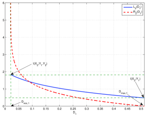
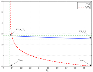
We illustrate our results for $\alpha=1,$ $\beta=8,$ $\sigma_{1}^{2}=0.05,$ and $\sigma_{2}^{2}=1.$ The parameters so chosen demonstrate the need for communication between the RTOs since at each RTO, there is interference from the measurements at the other RTO as well as noise. In Fig.  3, $R_{1}$ and $L_{1}$ are plotted as functions of $D_{2}$ while in Fig. 4, the effect of changing the distortion $D_{1}$ from its minimum to its maximum value on the rate $R_{2}$ and privacy leakage $L_{2}$ for RTO 2 are shown. The asymmetry in the interference and noise levels is captured in the two plots.

Figure 3: Plots of $R_{2}$ and $L_{2}$ vs. $D_{2}$.

Figure 4: Plots of $R_{1}$ and $L_{1}$ vs. $D_{2}$.

IV Concluding Remarks

In this paper, we have formalized the conflicting objectives of estimation accuracy and competitive privacy in smart-grid operations in terms of a class of information theoretic multi-terminal source coding problems. For a scalar Gaussian source model with two RTOs, we have completely characterized the set of optimal privacy-utility tuples via the rate-distortion-leakage tradeoff for a mean-squared estimation criterion. We have shown that the RDL tradeoff at each RTO depends only on the fidelity requirement at the other RTO with a higher fidelity requirement leading to a higher rate and higher leakage and vice-versa. While the results here also extend to vector Gaussian sources and a mean-square fidelity criterion, we intend to investigate the RDL trade-off for general non-Gaussian source models and multiple RTOs in a forthcoming paper.

Finally, we comment on some practical implementation issues associated with the proposed distributed formulation. While the optimal encoding strategies are necessarily block based, in practice it may not be feasible to accumulate the incoming data for long at each RTO and subsequently encode the entire block. A potential research direction would be the investigation of heuristic real-time encoding schemes that yield close to optimal performance with much less encoding complexity. Finally, a practical approach for the distributed and decentralized information broadcast in such multi-agent networks is via gossip protocols (see, for example, [14]).

References

- [1] A. Bose, “Smart transmission grid applications and their supporting infrastructure,” IEEE Trans. Smart Grid, vol. 1, no. 1, pp. 11–19, Jun. 2010.
- [2] F. F. Wu, K. Moslehi, and A. Bose, “Power system control centers: Past, present, and future,” Proc. IEEE, vol. 93, no. 11, pp. 1890–1908, Nov. 2005.
- [3] T. V. Cutsem, J. L. Horward, and M. Ribbens-Pavella, “A two-level static state estimator for electric power systems,” IEEE Trans. Power Apparatus and Systems, vol. 100, no. 8, pp. 3722–3732, Aug. 1981.
- [4] E. L. Quinn, “Privacy and the new energy infrastructure,” Social Science Research Network, Feb. 2009.
- [5] Guidelines for Smart Grid Cyber Security: Vol. 2, Privacy and the Smart Grid, National Institutes of Standards and Technology, Aug. 2010, http://csrc.nist.gov/publications/.
- [6] C. Efthymiou and G. Kalogridis, “Smart grid privacy via anonymization of smart metering data,” in Proc. IEEE 1st Intl. Conf. Smart Grid Comm., Gaithersburg, MD, USA, Oct. 2010, pp. 238–243.
- [7] G. Kalogridis, C. Efthymiou, S. Z. Denic, T. A. Lewis, and R. Cepeda, “Privacy for smart meters: Towards undetectable appliance load signatures,” in Proc. IEEE 1st Intl. Conf. Smart Grid Comm., Gaithersburg, MD, Oct. 2010, pp. 232–237.
- [8] H. Y. Lam, G. S. K. Fung, and W. K. Lee, “A novel method to construct taxonomy of electrical appliances based on load signatures,” IEEE Trans. Consumer Electronics, vol. 53, no. 2, pp. 653–660, May 2007.
- [9] S. Papadimitriou, F. Li, G. Kollios, and P. S. Yu, “Time series compressibility and privacy,” in Proc. 33rd Intl Conf. Very Large Databases, ser. VLDB ’07, Vienna, Austria, 2007, pp. 459–470.
- [10] R. C. W. Wong and E. Lo, “Competitive privacy: Secure analysis on integrated sequence data,” in Proc. Database Syst. Ad. Apps., Tsukuba, Japan, Apr. 2010, pp. 168–175.
- [11] V. Prabhakaran, D. Tse, and K. Ramachandran, “Rate region of the quadratic Gaussian CEO problem,” in Proc. Intl. Symp. Inform. Theory, Jun. 28-Jul. 2 2004, p. 119.
- [12] A. D. Wyner and J. Ziv, “The rate-distortion function for source coding with side information at the decoder,” IEEE Trans. Inform. Theory, vol. 22, no. 1, pp. 1–10, Jan. 1976.
- [13] T. M. Cover and J. A. Thomas, Elements of Information Theory, 2nd ed. New York: Wiley, 2006.
- [14] S. Boyd, A. Ghosh, B. Prabhakar, and D. Shah, “Randomized gossip algorithms,” IEEE Trans. Inform. Theory, vol. 52, pp. 2508–2530, Jun. 2006.