Implementing the Gaia Astrometric Global Iterative Solution (AGIS) in Java

Abstract

This paper provides a description of the Java software framework which has been constructed to run the Astrometric Global Iterative Solution for the Gaia mission. This is the mathematical framework to provide the rigid reference frame for Gaia observations from the Gaia data itself. This process makes Gaia a self calibrated, and input catalogue independent, mission. The framework is highly distributed typically running on a cluster of machines with a database back end. All code is written in the Java language. We describe the overall architecture and some of the details of the implementation.

1 Introduction

Astrometry is one of the oldest pursuits in science. The measurement of positions and later motions of celestial bodies has been an occupation for millennia. The most famous, but now lost, star catalogue of the Antiquity was compiled around 129 BC by Hipparchus (Schaefer, 2005), whose name is echoed in the Hipparcos mission (ESA, 1997) which brought the first space-based astrometry. Gaia continues in this ancient tradition using the most modern of techniques.

ESA is due to launch the $\sim$2000 kg Gaia satellite in 2013 on a Soyuz-Fregat rocket to the L2 point some 1.5 million km from earth. It consists of an astrometric instrument with two viewing directions, complemented by photometric and radial-velocity instruments providing astrophysical information and allowing it to build a phase-space map of our galaxy.

Over its five-year mission Gaia will obtain astrometric and photometric data for about a thousand million sources (stars, quasars, and other point-like objects); a subset of about 250 million of the brighter sources will also be observed spectrographically. Gaia will use a mosaic of CCD detectors operated in a drift-scanning mode throughout the five years, producing an average of approximately 700 individual CCD observations of each source and covering the entire sky three-fold every six months. For more detailed overviews of the Gaia project and its science goals we refer to, e.g., Turon et al (2005), Lindegren et al (2008), Jordan (2008), Lindegren (2010) and de Bruijne et al (2010).

A central part of the data processing for Gaia is the so-called Astrometric Global Iterative Solution (AGIS), which transforms the $\sim$$10^{12}$ individual observations into an astrometric catalogue of unprecedented accuracy. The full mathematical details of AGIS are given elsewhere (Lindegren et al, 2011) and are only briefly referred to below. In the present paper we discuss the overall architecture of the processing framework that is being set up to carry out this huge task, as well as some details of the implementation.

When reading this paper it should be borne in mind that the word Object will be used in the sense that is normal in computer science or object-oriented programming. It should not be confused with an astronomical object, for which, in general, we use the term Source. For improved clarity, names of classes and methods are generally set in italics when they appear in regular text.

2 The Gaia Astrometric Global Iterative Solution (AGIS)

2.1 Astrometry as a minimization problem

In ESA (1997) the general principle of a global astrometric mission is succinctly formulated as the minimization problem:

$$\min_{\vec{s},\vec{n}}\|\vec{g}^{\text{obs}}-\vec{g}^{\text{calc}}(\vec{s},\vec{n})\|_{M}$$ (1)

where $\vec{g}^{\text{obs}}$ is the vector of all the observations (measurements), $\vec{g}^{\text{calc}}$ the corresponding calculated values, and the norm is calculated in some metric $M$ that takes into account the different weights of the observations.

The vector $\vec{s}$ represents the (unknown) astrometric parameters of the sources. As described in detail in (Lindegren et al, 2011), each source $i$ is modelled in terms of six astrometric parameters, namely:

$\alpha_{i}$	right ascension at a given reference time, i.e., the longitude-like coordinate along the celestial equator
$\delta_{i}$	right ascension at a given reference time, i.e., the angular distance from the celestial equator (positive towards north)
$\varpi_{i}$	annual parallax, inversely proportional to distance from the sun
$\mu_{\alpha*i}$	($=\mu_{\alpha}\cos\delta$) proper motion in right ascension, i.e., the annual change in $\alpha$ times $\cos\delta$
$\mu_{\delta i}$	proper motion in declination, i.e., the annual change in $\delta$
$v_{ri}$	radial velocity, i.e., the rate of change of the distance to the source.

The radial velocity $v_{ri}$ is best determined spectroscopically, using the Doppler shift of spectral lines, and is not included among the unknowns to be determined by the astrometric solution. The vector $\vec{s}$ therefore contains 5 unknowns for each source. The astrometric solution will operate on a subset of about 10% of the sources known as the primary sources (see Sect. 7.5), so the total number of astrometric unknowns is some $5\times 10^{8}$.

The vector $\vec{n}$ contains the nuisance parameters, i.e., all other parameters that need to be determined simultaneously with $\vec{s}$, using the same observations, because they cannot be measured accurately enough by other means. These include the satellite attitude, the geometric calibration of the instrument, and a few global parameters. Their total number is of the order of $10^{7}$.

2.2 Iterative solution

Equation (1) means that the model, encapsulated by the function $\vec{g}^{\text{calc}}$, is fitted to the observations by adjustment of the parameters $\vec{s}$ and $\vec{n}$. To directly fit all parameters is infeasible, considering their number in excess of $n=5\times 10^{8}$. A brute-force direct solution would require about $n^{3}/6\sim 2\times 10^{25}$ FLOPs and the normal equations matrix would occupy about $n^{2}/2\sim 10^{17}$ doubles or 1 exabyte (1 million TB) of storage. Rather than a direct solution we take a block iterative approach.

We model the effects of the source, attitude, calibration and global parameters independently, treating the dependencies as given. Hence to solve for the astrometric parameters of a source we assume some attitude, calibration and global parameters; then for calibration we assume the global, attitude and astrometric parameters, and so on. The order in which this is done should in principle not matter although solving the astrometry for the individual sources first is logical and has some advantages (Sect. 7.5). Hence the solution would involve four relatively independent blocks of equations, where each takes the form of the general minimization problem of Eq. (1), although only for a subset of the parameters. The four blocks are referred to as the Source Update, Attitude Update, Calibration Update, and Global Update.

The convergence properties of this kind of (simple) iterative solution were essentially unknown when the Gaia data processing system was first planned. Although it was felt that it should converge, there was no proof of even that. The early work outlined in O’Mullane and Lindegren (1999) was a first indication that convergence in a few tens of iterations should be possible. Subsequent experiments have shown that the iterations do indeed converge, although slowly, and that the convergence speed can be improved considerably by modifying the updates to take into account previous updates. The current solution method, based on the conjugate gradients algorithm, converges and effectively removes all systematic errors in the initial catalogue data in some 40–100 iterations, when applied to simulated data (Bombrun et al, 2010). In practice one must iterate until the updates become very small, and further work continues to define an exact convergence criterion.

The efficient software implementation of the block iterative solution is challenging. A first attempt for such a solution during the Hipparcos data processing was abandoned. A basic proof of concept, actually more a pseudo implementation, using again Hipparcos data and a database management system, was presented in O’Mullane and Lindegren (1999). A good deal of effort went into scaling this up to Gaia dimensions until finally a degree of success was gained by the ESAC group (O’Mullane et al, 2006) in 2005. It is this ESAC framework which is presented here and which shall continue to be developed up to and even after the launch of Gaia.

3 Overview of the AGIS data processing system

AGIS is just one of many parts of the Gaia processing, a central or core part certainly but still a part. In the overall design of the Gaia processing system the Main Database is the central repository of all information. Figure 1 depicts AGIS is this broader context with the Main Database.

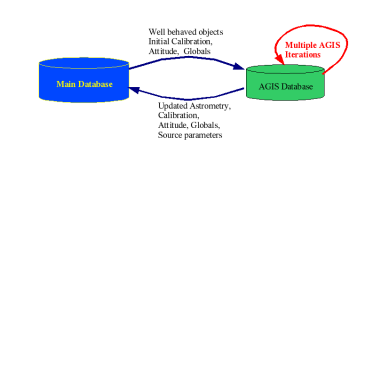
Figure 1: AGIS, like other Gaia processing systems, extracts data from the Main Database. Updated results are fed back to the Main Database and merged with results coming from other processing systems.

A simplified overall AGIS picture is presented in Fig. 2. Each of the components in the picture may run on practically any regular machine apart from the Attitude Update Server, which requires a little more memory (of the order of 16 GB). The DataTrain, as mediator, is seen in the middle of the left box and is explained in some detail in Sect. 4.3. The database systems – currently InterSystems Caché, Oracle Real Application Clusters, or (for small data sets) Apache Derby – may also run on several machines (or nodes) to improve data access performance. The data access and storage is abstracted through the Store interface which is described in Sect. 4.4. The algorithms and collectors are described in Sect. 7.

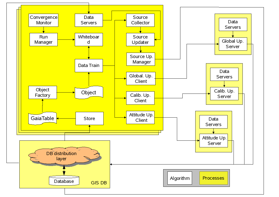
Figure 2: Logical overview of AGIS. The many processes of AGIS run on many different machines (not shown here). The large box on the left represents the DataTrain, of which there may be a great number running. On the right are the update servers, of which there may be only one of each kind running in the entire system. A database management system underpins all of these processes.

The AGIS system is deployed on a local multi-processor machine dedicated to Gaia. All the classes are available on each node but objects will be run on specific nodes according to the configuration specified in the agis.properties file. Objects on different hosts communicate through Remote Method Invocation (RMI), although we actually use JBoss remote-method calls for efficiency. This would be an ideal candidate for Enterprise Java Bean (EJB) implementation but we found EJBs very inefficient. In general a class with the name SomeServer will only have one instance on the cluster, while the DataTrain may have numerous instances, e.g., one on each node in the cluster. Internally the DataTrain makes use of multiple processors and cores available in a node.

4 Data access

The key to an efficient implementation of AGIS is in the data access. Even with today’s machines, accessing a large volume (tens of terabytes) in both spatial and temporal order is demanding.

4.1 Data access patterns

Looking at the four main blocks of AGIS we see that each has a seemingly unique data access pattern, viz.:

Source	All observations of a given source – spatial
Attitude	All observations within a given time period – temporal
Calibration	All observations within a given time period falling on a given CCD – temporal/spatial
Global	All observations – any order

(The ‘observations’ here refer to the AstroElementary objects described in Sect. 5.) The naive approach would be to go through the data once for each block, updating the parameters in turn and then repeating this for each iteration. This is indeed the basic mathematical formulation of the block-iterative solution method and the corresponding data access scheme is depicted in Fig. 3 (left).

    

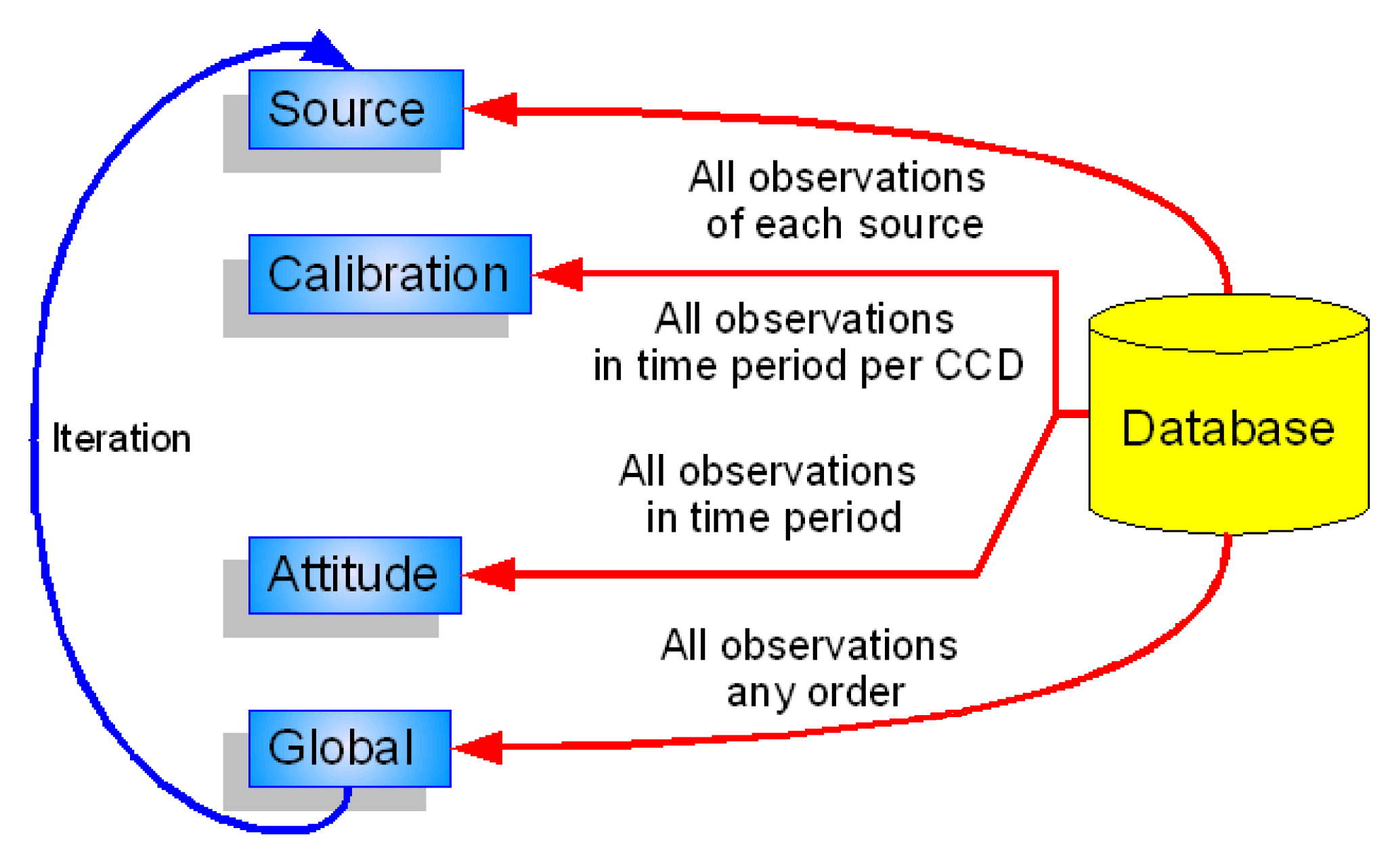
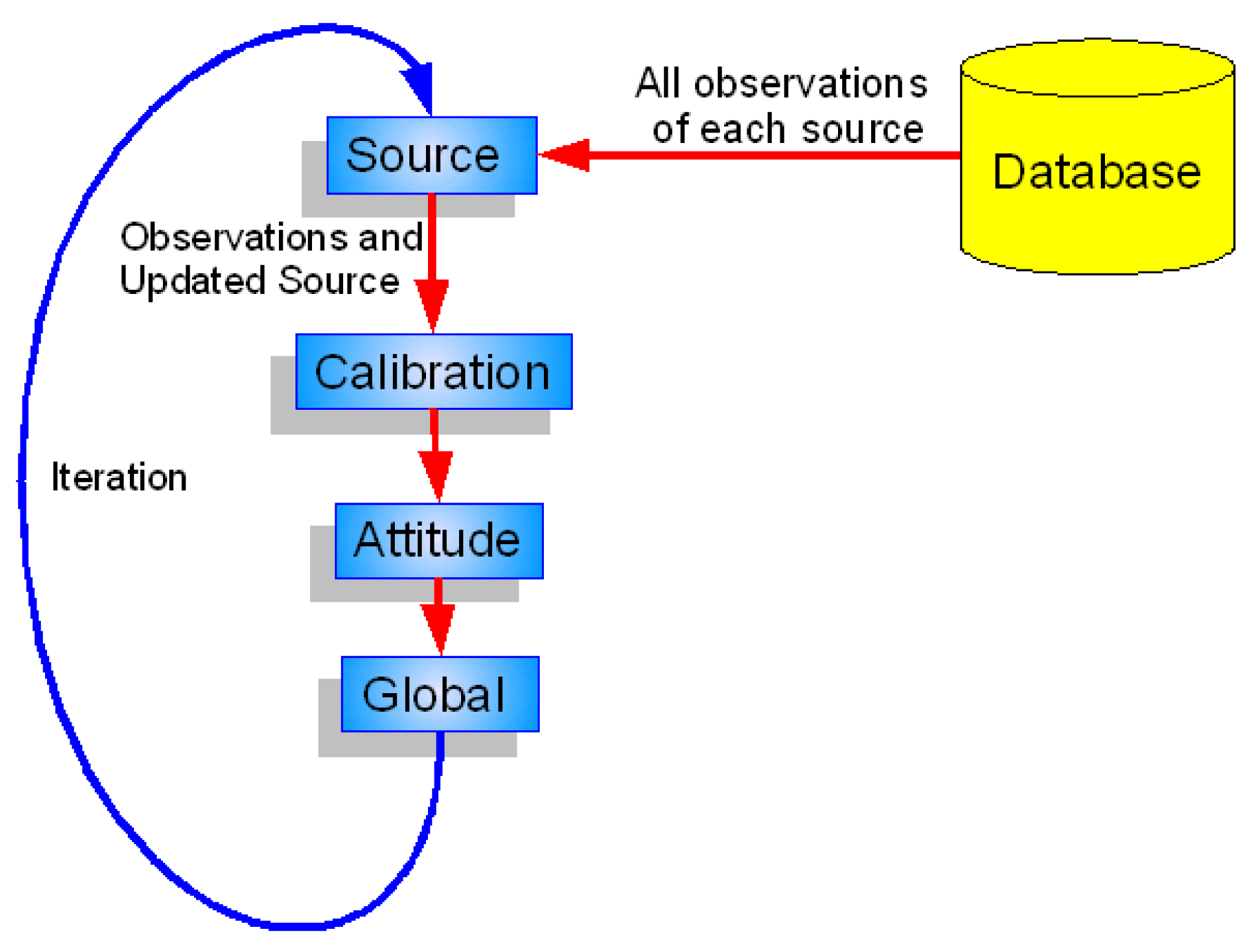
Figure 3: Left: Each block of the AGIS solution has a slightly different data access requirement. This could cause four passes through the data for each AGIS iteration. However, it is immediately clear that some of these could be combined, e.g., the calibration and attitude updates could run together, and similarly the source and global updates. Right: With a little in-memory accumulation in the calibration, attitude and global update blocks, a complete iteration can be made in one pass though the data. Hence the optimal ordering is spatial. Furthermore the updated source parameters may already be used in the other blocks.

Running through the approximately ten terabytes of data four times per iteration is rather daunting, considering that many tens of iterations will be needed. Immediately, though, we see that the calibration and attitude updates are similar enough that the can perhaps be combined. The global update is order-independent and as such could be combined with the data access of any of the other blocks, for example source. Indeed this was already remarked in O’Mullane and Lindegren (1999), where the prototype made just two passes through the data for each iteration rather than four. The question then is: could this be reduced to one pass through the data per iteration?

4.2 A question of order

Let us assume that all four blocks could be executed in one pass; what then would be the impact of the ordering of the data? There are two primary orderings we may choose: spatial or temporal.

Temporal ordering

If we assume an ordering based on the time of observation, then for the attitude we may read the data once, break it in time chunks suitable for the attitude update, process each chunk in turn and finish with it. With a small buffer we may also accumulate the observations required for the calibration and similarly finish with calibrations in a timely manner during the same pass through the data. For the global update the order is immaterial, so it can be done in parallel with the attitude and calibration updates.

The problem here comes with the source update. Since any given source is observed many times over the entire mission, if we process in time order we must accumulate the data for each source until we have all observations of it. This will not happen until we have seen all of the data – only then can we be certain that no more observations of a given source will show up. This would effectively mean that all observation data would end up in memory. For a hundred million sources (with almost $10^{11}$ observations) and some clever organizing this would be of the order of 5 TB of data, which is infeasible to have in shared memory on our budget. The final solution may require five times as many observations. The alternative is another pass through the data in spatial order. Since we must wait until the end of the first pass for the updated calibration, attitude and global parameters, these updated values could already be used for the source update.

Spatial ordering

If we assume a spatial ordering, i.e., that all observations of a source are clustered together, then the story is quite different. Now we may process each source to find its new astrometric solution, which can immediately be written out to disk. Since we are finished with that source, the updated parameters may be used to find its contributions to the global parameters. The situation for the attitude and calibration updates is however that all contributions from all observations must be accumulated until the end of the pass through the data – only then may the calibration and attitude updates be calculated. It is important to note that it is not the observations which must be held but their contribution to the matrices of attitude and calibration, which is much smaller than the accumulation of the source matrices in the temporal ordering. The entire attitude accumulation for the five year mission data can be done in 8 GB of memory. The size of the calibration matrix depends on the number of calibration artifacts – currently it requires about 4 GB but is estimated to need as much as 32 GB when additional calibration parameters are added in the coming years. Hence with spatial ordering one pass may be made though the data for each AGIS iteration, as depicted in Fig. 3 (right), and a minimum amount of data needs to be held in memory.

This clearly represents a better approach to the ordering from a technical point of view. Additionally, it is more natural to keep astronomical data of the same part of the sky together and easily accessible. Hence the AGIS database has observations of the same source sequentially grouped together on disk.

4.3 Getting data to the algorithms: the DataTrain and Taker

Throughout the Gaia processing there are choices to be made concerning data access patterns such as those outlined in Sect. 4.2. The ideal approach, for efficiency, is a data driven approach whereby data is accessed in the sequential order in which it is stored. Hence rather than algorithms requesting data they should be presented with data by a mediator. The mediator pattern (Gamma et al, 1994) is a very powerful tool for decoupling software modules. The implementation of the mediator for the astrometric solution is called the ElementaryDataTrain.

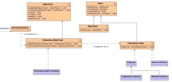
Figure 4: The DataTrain acts as a mediator between algorithms and data access (the Store) thus leading to a less coupled system. The ElementaryDataTrain accesses AstroElementarys in the fastest possible manner for the AGIS algorithms. The participating algorithms must implement the Taker interface.

The generic notion of a DataTrain (Fig. 4) is to access data in the fastest possible manner, usually meaning sequentially, and call a given set of algorithms passing them the data. The concept and code are quite simple. To enable the calling of the algorithms in a generic manner they must implement the Taker interface, which has a method to ‘take’ some data. By implementing this interface, the algorithm will have its input when it is called by the DataTrain.

More specifically, for AGIS the ElementaryDataTrain accesses AstroElementary objects, which are effectively the observations of a given source. The train decides which data to access by taking a Job (see Sect. 6.2). It uses the Store to access a set of AstroElementary objects, each of which is then passed to each registered ElementaryTaker, i.e., the source, attitude, calibration and global update algorithms. Each algorithm (see Sect. 7) must implement the ElementaryTaker interface to allow the DataTrain to interact with it. The ElementaryDataTrain has a method for registering the algorithms (addElementaryTaker in Fig. 4). The algorithms must then accumulate observations until they can process a particular source or time interval. This forces the algorithms to accept data in the order it is stored allowing the infrastructure to be built without fixing the data storage order. Choosing spatial ordering (Sect. 4.2) means that all of the elementaries for a given source are sequential. Any given train accesses complete sets of elementaries with respect to sources. The cartoon in Fig. 5 depicts this in a another manner showing how the AstroElementary is constructed by the ObjectFactory from a GaiaTable resulting from a query to the database through the Store interface. The AstroElementary is then passed to the algorithms attached to the DataTrain.

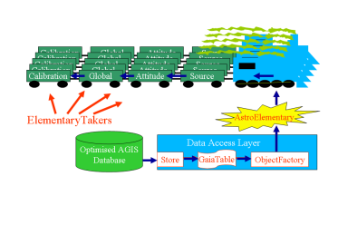
Figure 5: Here the blue arrow shows the flow of data from the database through the Store and ObjectFactory to the algorithms attached to the ElementaryDataTrain. We may think of the ElementaryDataTrain as driving through the database, passing observations to the algorithms. We may have as many trains in parallel as we wish.

4.4 Abstraction of data storage: the Store

To give a degree of independence from the physical storage mechanism, it is normal to use some abstraction. Java interfaces provide an excellent approach to provide such insulation. Creating an interface is a small coding overhead, while in usage one gets a real implementation, i.e., without overhead. It is very important to realize that a Java interface is a contract binding the using class and the providing class but does no translation of any kind. This should not be confused with rooted persistence systems requiring all classes to inherit from some root class. Here we simply have to implement a few methods implied by the interface. They are more for our convenience than a design principle – we also like to keep clear in our code which objects we will be storing and which we will not. It is also useful in the ObjectFactory to have a base interface to cast to, other than Object. We are not far from Java Persistence Architecture (JPA) in both principle and implementation – this however was not mature when we started in 2005. More recently we have considered simply switching to something like Hibernate but found the offerings far slower than our own system. We could remove the restriction of having GaiaRoot but it has not been a pressing issue to date. Having our own Store also made it easy to build a CacheStore which took advantage of the Cache high speed interface, they do not support JPA.

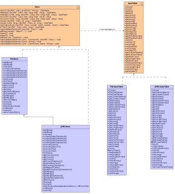
Figure 6: The Store provides an interface for data access, whereby many Store implementations may exist. In the Figure we see a FileStore and a JDBCStore, both of which implement Store. With these implementations of AGIS code we may switch between FITS files and a JDBC Database for storage in a seamless manner.

No algorithm code in the system interacts directly with the database management system; rather a query interface to the data is provided through the Store interface (see Fig. 6). The implementation of the Store is hidden behind the interface; thus the data store may be implemented in files or any database management system.

An implementation of the Store is requested from the AGISFactory, the actual implementation of the store is configured using the gaia.tools.dal.Store property in the agis.properties file and thus can be changed at run-time (rather than at compile-time). The Store interface includes an explicit range query which returns all objects within a certain id range, which is required to support the DataTrain.

As depicted in Fig. 6 there are multiple implementations of the Store. The FileStore does not support the same level of querying as the JDBCStore but is sufficient for running the testbed on a laptop. Most recently we have also implemented a CacheStore over the InterSystems Caché database.

GaiaTable in Fig. 6 represents an interface to tabular data. The assumption of dealing only with tabular data is a major simplification for AGIS. This is a fair assumption dealing with astrometry data. Both files (be they FITS or whatever) and relational database tables may be represented as a GaiaTable. The interface defines methods for retrieving the next row and for getting columns by name or index. The whole row may be passed to the algorithm or ObjectFactory and it may extract the required columns. The DataTrain loads the entire row.

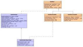
Figure 7: All data objects implement GaiaRoot, which makes certain methods available to the Store. All data objects are interfaces, not real classes – this allows them to be easily replaced by different implementations.

The GaiaRoot UML (Unified Modeling Language) diagram is given in Fig. 7. Color interfaces are shown in brown colour (and are also marked with a $\circ$), while implementations are in blue. Any objects in the Gaia data model which use the Store (see also Fig. 6) and ObjectFactory must implement this interface. A basic implementation is provided which most classes may inherit from, but in some cases, due to single inheritance in Java, this may not be possible. In fact practically all of the required functionality is in the Store or ObjectFactory.

Interfaces were chosen for the data classes originally, since the first implementations in 1998 used Objectivity/DB (from Objectivity, Inc.) which was a rooted system, thus requiring the objects to actually inherit from the Objectivity/DB base class. Even then the Store was working both with Oracle Real Application Clusters and Objectivity/DB, which meant having two implementations of the data objects. These days we usually only have one implementation; however, there are instances where the interfaces are still useful. For example higher-level classes such as AstrometricSource can have multiple subclasses. These may not follow the same inheritance hierarchy but can still be AstrometricSources since it is an interface; if it were only a class there could be inheritance problems.

4.5 Access to objects: the ObjectFactory

The Store deals essentially with tables but some code will require objects. The ObjectFactory sits on top of the Store and returns objects implementing the data model interfaces. The object-from-table method of the interface is also exposed, allowing code to do this conversion exactly when required. We need to take care that not too many pieces of code perform such a transformation – preferably it would be done once by the DataTrain. Splitting this out allows for very direct measurement of the performance.

This is implemented as a Generic class. The Factory is instantiated for a specific data model interface and then provides a method returning that class of object only. Java Generics are very nice for this and, although similar to C++ templates, should not be confused as being the same. Generics provide type checking and safety but they do not generate extra code with new types.

The Factory relies on the populate method of the GaiaRoot to populate the fields of the object from a GaiaTable. A generic implementation of this using a mapping from the configuration file is provided in the GaiaRootImpl class. This provides a convenient mechanism to read the data from the Store into a Java object that can be used elsewhere in the system.

The ObjectFactory also has caching capabilities. Whenever an object is read from the Store it may be cached in memory in order to avoid new reads when it is requested again. Any object which is created by the ObjectFactory can be made cacheable just by implementing the gaia.tools.dm.GaiaRootCacheable interface. The caching can also be disabled by adding an entry to the property file. The interface contains a method to determine the ‘validity’ of the object.

The Factory also has the possibility to implement object pooling. The notion here is to reuse objects by filling them with new data rather than reconstructing new ones. This technique was very popular in early Java implementations to reduce garbage collection time. Tests with the new JDK (1.5 and 1.6) show that this is no longer beneficial. Still, by having all data object creation done through one class the possibility to change the way it works later remains available.

5 The Data Model

The algorithms work in terms of Java objects such as Source and AstroElementary. These objects form what is generally termed a Data Model for the system.

The data used for AGIS will comprise between 10% to 50% of the sources (and their corresponding observations), corresponding to the so-called primary sources briefly discussed in Sect. 7.5. The selection of the primary sources is described in Lindegren et al (2011) and is implemented as several database queries. The selected data will be put in the special AGIS database (see for example Fig. 5).

The data model is made in terms of interfaces to allow easy substitution of multiple implementations. The ObjectFactory (Sect. 4.5) and Store (Sect. refsect:store) are used to construct real implementations of these interfaces but all code refers only to the interface. Hence all client code may be compiled without any implementation if necessary. This is a technique used throughout AGIS and indeed also for GaiaTools, the common software toolbox for all Gaia processing tasks. The most important interfaces are:

• AstroElementary: An object of this kind represents the transits of a celestial source over the first dedicated 10 CCD strips of the focal plane, namely, SM1 or SM2 and AF1–9 (see Lindegren et al, 2011, for an outline of the CCDs in the focal plane). Each AstroElementary in AGIS is uniquely associated with a Source.

• Source: An object of this kind represents celestial sources that follow the standard astrometric model (thus modelled by the six astrometric parameters described in Sect. 2.1) and are eligible for AGIS source processing.

• Attitude: An object of this kind represents an interval of continuous attitude data. Attitude is parametrized using B-spline coefficients of a given order representing the four components of the attitude quaternion (Sect. 7.2).

• CalibrationEffect: The geometrical calibration of the instrument is made up of multiple CalibrationEffects (Sect. 7.3) all of which may be configured in an XML file.

Table 1: Evolution of AGIS performance during the development of the processing framework. Data volumes are indicated by the number of observations (AstroElementaries), depending on the number of sources and the length of the observation period. The time is the processing time per AGIS iteration for the given number of processors. The last column shows the throughput, in observations per processor per hour, as an indication of the real performance.

Date	Observations	Processors	Time (hr)	Normalized Rate
2005	$1.6\times 10^{7}$	12	3	$0.9\times 10^{6}$
2006	$8.0\times 10^{7}$	36	5	$0.5\times 10^{6}$
2007	$8.0\times 10^{7}$	24	3	$1.3\times 10^{6}$
2008	$8.0\times 10^{7}$	31	1	$3.2\times 10^{6}$
2009	$2.6\times 10^{8}$	50	1.8	$2.8\times 10^{6}$
2010	$4.0\times 10^{9}$	68	9.5	$6.2\times 10^{6}$

6 Distributed processing

Regardless of the ordering chosen (Sect. 4.2) the access of the data does not need to be done serially. Indeed we require the data to be sequential on disk but multiple parts of that sequence may be read simultaneously. In the case of sources we may process simultaneously each source, in terms of distributed computing this is ‘embarrassingly parallel’ Wilkinson and Allen (1999). We may theoretically gain up to a factor $N$ in speed by using $N$ processors, if $N$ is the number of sources to be processed. We say theoretically with reason, as the data must still be read from disk and we are unlikely to actually put in place $10^{8}$ processors. Still, tests have shown that the processing time indeed decreases in proportion to the number of processors used for AGIS. Some numbers are given in Table 1.

6.1 Distributed processing frameworks

Many different approaches exist for distributed processing, and they are usually embodied in some library. However since we have an ‘embarrassingly parallel’ problem we have little need for such a complex and heavy library. In fact all that we require is already available within the standard Java library, namely:

• Communication between processing nodes: the Remote Method Invocation (RMI) framework in Java provides this.

• Access to a database or databases: the Java Data Base Connectivity (JDBC) framework provides this.

• Some form of graphics library for GUIs: Java Swing library provides this.

Additionally, in this age of the web, Java provides easy support for dynamic web site generation using Java Server Pages (JSP).

Hence an early feeling was to use the tools of Java directly, rather than try to fit the problem into one of the many distributed programming libraries, each with their own assumptions and problems. The modern programming languages of the day, such as Java, are very sophisticated in the feature set and tools they provide. For example the Java/Jini Parallel Framework (JJPF; Danelutto and Dazzi, 2006) provides some reliability on top of these tools while also taking a much more process-oriented view – each worker has a getData call to pass back results. JJPF is also more coordinator oriented with a single server eliciting support from available nodes to perform a computation. In the grid world the obvious contender would be the Globus Toolkit (GTK; Foster, 2006). Previous forays into GTK showed the system to be buggy and difficult to use. GTK has improved dramatically over the years, yet it still remains service oriented (we believe our problem to be data oriented) and has a large security overhead which we do not see as necessary. Indeed though Demichev et al (2003) is positive about GTK they introduce a resource broker which seems similar to our whiteboard (Sect. 6.2). Unfortunately say little about the data intensive applications mentioned in the title of their paper.

The notion of just using the Java framework without some other layer was reinforced by previous experiences with the Sloan Digital Sky Survey (SDSS). On the SDSS a form of distributed query system known as CasJobs (O’Mullane et al, 2005) was built using Web Services, the SQLServer database and the C# language. This was done quite rapidly without using any special libraries beyond the facilities available in the programming language. Within the same group at Johns Hopkins a typical Grid application for finding galaxy clusters in a large catalogue was taken and quickly rewritten in C#. As reported by Nieto-Santisteban et al (2005), this ran about ten times faster using a database system than the traditional file-based Grid system.

A final justification, perhaps the ultimate and obvious one, for not taking on a library is that of simplicity. It was believed the distributed computing libraries would not make the system simpler hence none were adopted.

6.2 Job distribution: the Whiteboard

There are at least two main approaches to controlling a grid of distributed processes. The first is to have ‘agents’ register with some central controller which then regulates the entire process; the second is to have a less centralized approach with more autonomous processes.

The central controller approach is very appealing and generally the way many agent-based systems work. Generally these involve monitoring resources and farming out jobs to particular processors which are not fully loaded. The central registering of agents means the controller knows how many agents of which types exist on the system, and furthermore may reject agents from particular machines or of particular types. Such systems deal well with uneven workloads and ad hoc jobs by many users. Often security layers and user tracking are included.

By contrast, an AGIS iteration could easily occupy an entire cluster for some days. There are no ad hoc programs, only the entire AGIS chain running on all data. There are no users, hence no particular need for a security overhead in terms of certificates, etc.

In our data driven approach (Sect. 4.3) we may consider the data as the distribution mechanism. Everything hinges on the processing of some block of data, be it a time sequence or a set of spatially ordered observations (Sect. 4.2). All we really need to know is if a particular part of the data set has been visited during a particular iteration. If the data segments are chosen properly we may have as many DataTrains running as we wish. This is very simple and easily achieved through a whiteboard mechanism as depicted in Fig. 8.

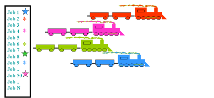
Figure 8: A set of jobs corresponding to sequential batches of data which cover the entire data range may be posted on a whiteboard (left). The DataTrain marks a job as in progress when it starts it and as completed when it is finished. There may be many DataTrains (right). When all jobs are done all of the data have been seen once. The whiteboard itself has no special knowledge of the jobs or the overall task – it is a simple mechanism to coordinate potentially hundreds of processes.

The whiteboard is quite a simple concept for organizing many processes of varying types. Conceptually we may ‘post’ jobs on a whiteboard, and then workers, in our case DataTrains, may pick them up. The whiteboard may hold status information, e.g., about when a job started, when it ended, if all was OK, etc. In effect then the whiteboard becomes the central controller, although it exercises no control as such. Perhaps the original of the species in this respect is the OPUS pipeline from the Space Telescope Science Institute (Rose et al, 1995). Indeed, it is the OPUS blackboard design pattern which is employed here. It is noted that since its early beginning, OPUS is itself moving toward Java (Miller et al, 2003) but maintaining its heterogeneity through CORBA (Common Object Request Broker Architecture). For the purposes of AGIS, which is a pure Java implementation, a simple Whiteboard was coded directly in Java using a database table to hold the jobs. The latter also provides the ability to ensure that no two trains ever get the same job. The JDBC framework in Java makes the whiteboard seamlessly accessible from any node on the network – hence no need for the overhead of CORBA or some other message passing system here. The UML interface for the Whiteboard is shown in Fig. 9.

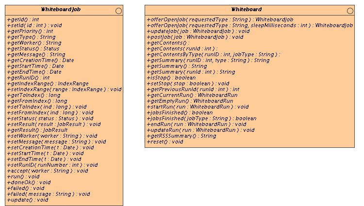
Figure 9: The UML interfaces for the Whiteboard and the WhiteboardJob. Note the postJob method used to populate the whiteboard and the offerOpenJob methods which the DataTrains use to get jobs. The job itself has methods for status and messages, etc.

Regardless of the jobs being done, the whiteboard can give some information on the general state of the system. A Series of JSP pages present the whiteboard state on a website. On this site with little effort we may show jobs completed/remaining and (assuming uniform jobs) an estimate for the end time. We may also list statistics per processor simply by querying the job table in the database.

6.3 Overall control: the RunManager and ConvergenceMonitor

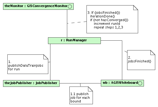
Figure 10: Communication diagram for the RunManager. This summarises the RunManagers role in publishing jobs and checking for convergence.

The Whiteboard alone is not enough to run an AGIS solution. Some other entity must post the jobs on the board for the DataTrains to work on. The RunManager has the task of coordinating iterations and the publishing of jobs as depicted in Fig. 10. The RunManager uses the JobPublisher to publish appropriate jobs, e.g., one for each block of sources to be processed. The JobPublisher scans a table of bounds (a list of identifiers of elementaries which are the last in a series belonging to a single source) and creates a number of jobs based on blocks of elementaries. In general the system is configured such that these jobs complete in a few minutes, as this gives a better indication of progress and the need to redo a job, in case of a problem, is detected in a timely manner. Hence there are typically thousands of jobs in a single run. Once posted, the trains pick them up and start working. The order in which the jobs are done does not matter. Jobs are also published for the calibration, attitude and global updates if these algorithms are attached to the train. These jobs execute for the entire iteration.

The RunManager then periodically checks to see if the DataTrain jobs have finished. If they are done the main part of the iteration is done, and the GisConvergenceMonitor is told the iteration is at an end. The RunManager then asks the GisConvergenceMonitor if the solution has converged and awaits the answer. At this point the attitude, global and calibration servers still must perform their final calculations – when these are complete the GisConvergenceMonitor reports the state of convergence. The convergence criterion is currently based on the typical size of the source updates in the current iteration.

If convergence has not been reached the RunManager starts another run through the data by publishing a new set of jobs. If it has converged the RunManager declares the run ended and converged.

7 Algorithms

There are effectively two types of algorithm in the system: those with a centralized part and those which are completely distributable. Let us first look at the source update algorithm which is completely distributed and subsequently at the others. The mathematical formulation of the algorithms (or blocks) is given in Lindegren et al (2011). As explained in Sect. 2.2 the blocks are iterated until the solution is considered converged.

7.1 Source update

The mathematical details of the source update are provided in Lindegren et al (2011). Very briefly, the update for source $i$ is obtained by solving the overdetermined system of equations

$$\vec{A}_{i}\vec{d}_{i}\simeq\vec{h}_{i}\,,$$ (2)

where $\vec{d}_{i}$ is the $n$-vector of updates to the astrometric parameters $\vec{s}_{i}$ of the source (usually with $n=5$, as described in Sect. 2.1), $\vec{h}_{i}$ the $m$-vector of residuals, where $m\gg n$ is the number of observations of the source, and $\vec{A}_{i}$ the design matrix. The problem is complemented by an $m$-vector of measurement uncertainties, $\vec{\sigma}_{i}$. The residual vector $\vec{h}_{i}$ contains the observed minus the calculated values for the source, such that the $j$th element is $h_{j}=g_{j}^{\text{obs}}-g_{j}^{\text{calc}}(\vec{s}_{i},\vec{n})$, $j=1\dots m$, where $g_{j}^{\text{obs}}$ is the observed position of the source on the CCD and $g_{j}^{\text{calc}}$ the calculated position based on the current best estimate of the source parameters $\vec{s}_{i}$ as well as the attitude, calibration and global parameters in $\vec{n}$, cf. Eq. (1). The elements of $\vec{A}_{i}$ are $A_{jk}=\partial g_{j}^{\text{calc}}/\partial s_{k}$ for $j=1\dots m$ and $k=1\dots n$. Each AstroElementary, consisting of up to 10 CCD transits, generates several rows of design equations.

The least-squares solution of Eq. (2) is by itself an iterative process, in order to have a self-adapting system of observation weighting (essentially by adjusting $\vec{\sigma}_{i}$) that is robust against outliers. Typically three or four such internal iterations are needed to compute the update $\vec{d}_{i}$, after which the improved source parameters are obtained as $\vec{s}_{i}+\vec{d}_{i}$. The solution of Eq. (2) is done in a very standard fashion by forming normal equations (Björck, 1996), which is computationally very efficient.

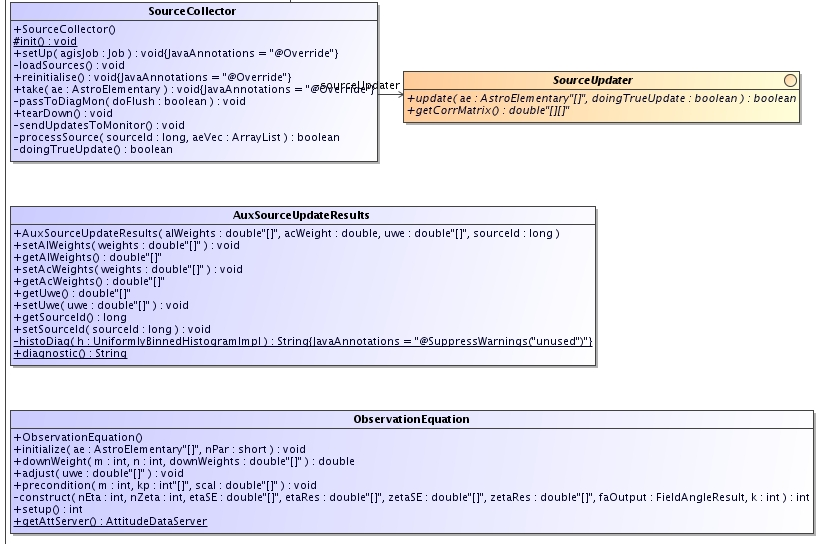
Figure 11: The SourceCollector is attached to each DataTrain and has a SourceUpdater associated with it to update all sources on disk when a job is finished.

The source update step is truly distributed. As the DataTrain passes elementaries to the SourceCollector (the Taker registered with the train for sources) it accumulates all of the elementaries for a given source. Remember that the data are stored in such a manner that all elementaries for one source are consecutive; hence, when the sourceId changes, the collector knows that it has all the data for a given source. Once it has a batch of elementaries, the source update is called to compute the required update of the astrometric parameters.

Figure 11 provides a UML overview of some of the classes involved in the source update. When the updated astrometric parameters are available they are passed to the SourceUpdateManager, which batches together several sources for efficient storage. Nothing in AGIS is ever actually updated, rather a new source row is written to the table with the current runId. In this way a complete history of the updates are preserved. Inserting to the database is also more efficient than updating.

In fact the SourceUpdateManager does not write the sources finally until the entire job is done. When all sources are updated a database transaction is opened to write all the results – only when this is done is the job considered finished. In this manner a job is either completed or not, since the transaction may be ‘rolled back’ without consequence if there is some problem.

When the job is finished the SourceCollector sends all of the updated sources to the GisConvergenceMonitor. This call is made using RMI. Because the GisConvergenceMonitor receives sources throughout the iteration, histograms of the updates can be dynamically generated. These are displayed on the associated AGIS website in real time. An example of the website is shown in Fig. 12.

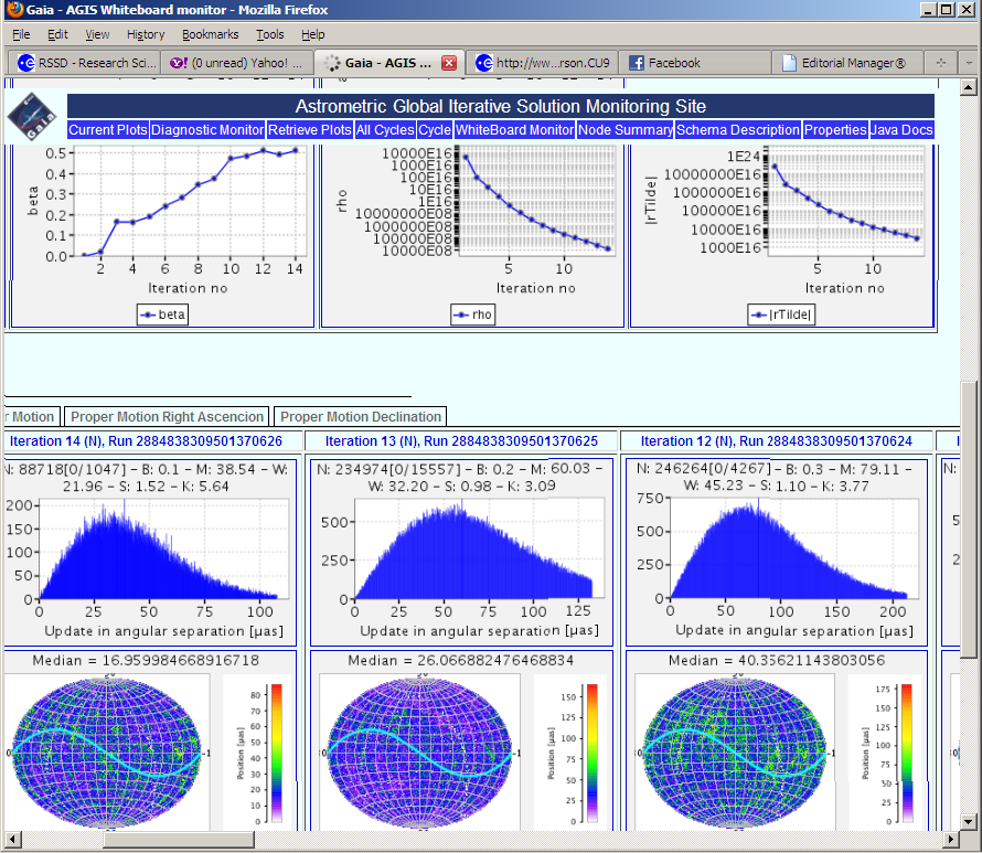
Figure 12: Update plots such as for the source position update shown here are generated dynamically and displayed on the AGIS monitoring website while the system is running. The Conjugate Gradients parameters such as $\rho$ and $|\vec{\tilde{r}}|$ (see Lindegren et al, 2011, for details) are also tracked as shown. Historical plots may be retrieved from the system.

7.2 Attitude update

The attitude specifies the instantaneous orientation of Gaia in the same celestial reference frame as used for the astrometric parameters – for Gaia this is known as the Center-of-Mass Reference System (CoMRS). Being the local rest frame of Gaia, the axes of the CoMRS are aligned with the International Celestial Reference System (ICRS; Feissel and Mignard, 1998), but with Gaia as the origin of the coordinate system instead of the solar system barycentre (Fig. 13). While the CoMRS is an inertial frame, the Scanning Reference System (SRS) rotates with the satellite and the optical axes of the astrometric telescope are fixed in the SRS. To a first approximation, the CCDs therefore measure the positions of the sources in the SRS.

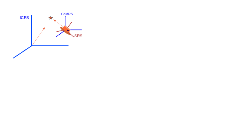
Figure 13: The position of a source is initially given in the ICRS, centred on the solar-system barycentre, and is then transformed to the Gaia-centred CoMRS by taking into account parallax and relativistic effects. Finally the position may be transformed to the SRS (Scanning Reference System), which is fixed to the spinning instrument, by means of a rotation given by the attitude quaternion $\vec{q}$.

The CoMRS and SRS frames are related by a purely spatial rotation, which defines the instantaneous attitude of Gaia. We use quaternions (Hamilton, 1847) to represent the attitude, as is common practice for spacecraft (e.g., Kane et al, 1983). The quaternion ${\bf q}$ is a 4-vector representing a direction in space (expressed in either the CoMRS or the SRS) and an angle of rotation around that direction. The four elements of the quaternion are continuous functions of time, here denoted $q^{k}(t)$, $k=1\dots 4$, which allow a singular-free attitude representation for arbitrary rotations. These functions are modelled as cubic splines, using short-range B-splines $B_{n}(t)$ as basis functions (de Boor, 2001); thus

$$q^{k}(t)=\sum_{n}a_{n}^{k}B_{n}(t)\,,$$ (3)

where $a_{n}^{k}$ are the attitude parameters, of which there are a few million in the system Lindegren et al (see 2011, for details). The attitude update solves a linearised least-squares problem similar to Eq. (2) but with the unknowns $\vec{d}$ now being the updates to the attitude parameters $a_{n}^{k}$ and the partial derivatives in $\vec{A}$ being taken with respect to these attitude parameters. The dimension $m$ is however very much greater in this case, since the attitude update in principle has to consider all the observations throughout the mission. However, thanks to the short range of the B-splines, the attitude normal matrix is band-diagonal, and the resulting system can be stored and solved very efficiently.

In fact the attitude may be divided into segments each of which can be solved simultaneously but separately. There will be natural breaks in Gaia’s attitude that can be used to segment the data, but this technique may be used to distribute the attitude processing further. Hence, depending on the number of attitude segments, there is a limit to the distribution of attitude processing. Each segment may be solved on an individual processor. In actual fact the final fitting of the attitude for five years data as a single spline with knots every fifteen seconds took only 30 minutes on a Xeon processor with 16 GB of memory. The solution itself is not the bottleneck, but rather the gathering of the observations. With a single attitude update server all source observations must be passed to this server from every data train. Once the system surpassed 32 DataTrains this became a limiting factor.

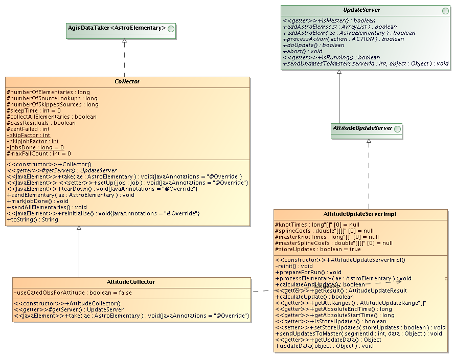
Figure 14: UML diagram for the distributed attitude update. The calibration update has similar classes.

On each data train an AttitudeCollector is registered. This gathers all of the elementaries and passes them to the appropriate AttitudeUpdateServer. Appropriate here means the attitude server dealing with the time bin in which the observation falls. In some cases the segments overlap and an observation must be sent to two servers simultaneously. Again RMI is used for this passing and the observations carry the updated source parameters with them.

The AttitudeUpdateServer(s) adds to the partial equations for each observation passed. It must wait until the end of the run to ensure all observations have been seen before doing the final computation. The end of the run is signalled, via RMI, by the RunManager. At this point the updated spline coefficients are calculated and written to the Store. The server also now sends the updated attitude to the ConvergenceMonitor so it may be plotted on the website.

7.3 Calibration update

The geometric calibration model deals with the precise placement and orientation of the CCDs in the focal plane. Within the optical system light bounces off six highly polished mirrors before hitting the CCDs in the Focal Plane Assembly. Since there are no on-board calibration devices a distortion in a mirror is indistinguishable from a displacement of a CCD. In both cases the image centroid will not appear where it should be. This also means that any such shift can be modelled in terms of CCD orientation, ignoring the mirrors entirely, and this is precisely what we do in AGIS.

Geometric calibration parameters for the CCDs, such as orientation, scale and mechanical distortions, are defined on timescales of hours or months as needed and are know as CalibrationEffects. This transformation for Gaia is quite involved Bastian and Biermann (see 2005), yet for our purposes we may consider an instantaneous position $\eta^{\text{obs}}$ for the source in the field of view. We define the astrometric calibrations in the following generalised form:

$$\eta^{\text{obs}}_{l}=\eta_{n}^{0}+\sum_{r}E_{r}(l)\,,$$ (4)

where $l$ is the observation index and each of the $E_{r}(l)$ represents one basic CalibrationEffect, being a linear combination of calibration functions $\Phi_{rs}(l)$:

$$E_{r}(l)=\sum_{s}c_{rs}\Phi_{rs}(l)\,.$$ (5)

The coefficients $c_{rs}$ constitute the whole set of calibration parameters. In the calibration update we solve these coefficients by a least-squares system similar to Eq. (2).

The functions $\Phi_{rs}$ receive the observation index $l$ and it is assumed that this index suffices to derive whatever dependencies are needed to evaluate the corresponding function/effect for this observation. Examples of such dependencies are: the telescope index (preceding/following field of view); CCD row number; CCD strip number; pixel column within the CCD; time; relevant astrometric, photometric, and spectroscopic source parameters; auxiliary parameters (e.g., optical background level, illumination history of the pixel column). In this generic calibration scheme the dependencies are not hardcoded, and we do not know exactly how many calibration parameters there will be in the mission. Furthermore the calibration effects are all specified in an XML file allowing for easy addition (or removal) of specific effects in an AGIS execution.

Following the terminology introduced in Lindegren et al (2011), the calibration parameters can be grouped into calibration units that can be handled separately because any given observation $l$ can only belong to one calibration unit. Within a calibration unit, on the other hand, each observation typically contribute to many different effects, for example to irregularities both on a large scale (e.g., between CCDs) and on a small scale (e.g., between pixel columns). Our estimate is that no calibration unit will have more than about 10,000 parameters, which is negligible compared to the attitude parameters. Still, the memory requirements in the calibration block are larger than in the attitude update because there is no obvious way to exploit the sparseness of the normal matrix within each calibration unit. The CalibrationEffects are depicted using UML in Fig. 15.

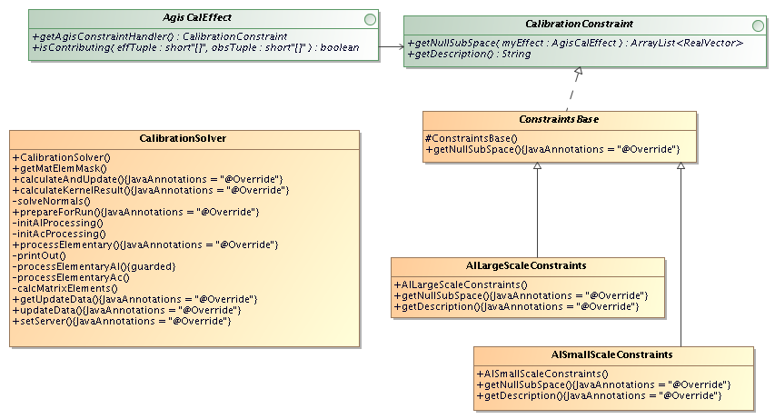
Figure 15: UML for the CalibrationEffects

From the perspective of distributed processing one must consider that, unlike attitude, here an observation will end up going to many calibration effects, e.g., both the large-scale and the small-scale calibration. We may however process all effects for a row of CCDs on a separate machine. The processing for calibration is not a huge overhead; as for attitude, the main bottleneck is the sending of all observations to the calibration server(s). Unlike the attitude, the calibration server can process the incoming observations more quickly and it has not been an overall bottleneck in the system.

The framework is similar to that of the attitude update. A CalibrationCollector is registered with each DataTrain, collects the required observation information and sends it to the CalibrationUpdateServer via RMI. The server accumulates the equations during the run and performs the final calculation when signalled by the RunManager that the run is complete. It writes the updated calibrations to the Store and sends them to the GisConvergenceMonitor for plotting on the website.

7.4 Global update

The global parameters, nominally some of the Parameterized Post-Newtonian (PPN) relativistic parameters, are estimated using a robust least-squares algorithm similar to Eq. (2) but now involving all the observations but only a (very) small set of parameters. The treatment is practically identical to a calibration parameter which spans the entire mission. As such it would be possible to combine this with the calibration update in a later version of the system, but for other reasons it is convenient to separate these terms, for example, to more easily estimate their correlations. As in the case for the attitude and calibration blocks we also have a GlobalCollector and a GlobalUpdateManager functioning in the same manner as described previously.

We will have sufficient observations and full sky coverage to decouple the global parameters from the astrometric parameters. Currently we only calculate PPN-$\gamma$ due to solar system body deflection, but other variants will be added in the future, for example, separate and combined values of PPN-$\gamma$ due to deflection by the major planets. The calculation of additional global parameters can provide a sanity check on the entire solution, i.e., a value wildly departing from the nominal value in the simulation data can only mean we are doing something very wrong somewhere.

7.5 Secondary source update

Nominally the entire data set could be put through AGIS, however we know that many binary stars and other complex objects will not work well with the simple observation model used. Hence only a fraction (between 10 and 50%) of the sources observed by Gaia are processed in AGIS. The selection of these primary sources will be done partly based on information from other parts of the processing chain (e.g., detected double stars), but mainly from the goodness-of-fit statistics gathered while performing a trial source update. If the fit is bad for the source, it is not accepted as a primary source but relegated to secondary source status. The selection of primary/secondary sources is itself an iterative process, which must be repeated after more accurate estimates have been obtained of the attitude and calibration parameters.

The AGIS solution, thus based on a ‘clean’ subset of the sources, provides an accurate celestial reference frame along with a correspondingly accurate attitude and geometric calibration. These outputs will be used to update the remaining fraction of the sources. This secondary star update is effectively identical to the source update block described in Sect. 7.1 but must only be run once over the data. This secondary solution will still not make sense for all types of objects (e.g., resolved binaries), which will be picked up in other parts of the processing chain.

8 Results

Some run times for the system are given in Table 1. AGIS has been running almost continuously since the end of 2005 on different simulated data sets. The current system requires around 40 iterations to remove initial (random and systematic) catalogue errors of about 100 milliarcseconds, based on the simulated observations. This level of initial errors is well above expected mission levels. After 40 iterations AGIS the source errors have been reduced to a level that is consistent with the observational noise level, i.e., some microarcsec for the brighter sources. Moreover, none of the systematic errors introduced in the starting values remain in the converged solution. A more comprehensive study of the results from AGIS will be provided in another paper.

9 Conclusion

The overall AGIS architecture and many of the components have been described in some detail. This is a software system designed and optimised to perform the Gaia astrometric data reduction involving the solution of a system with hundreds of millions of parameters and hundreds of billions of observations.

Advanced features of the Java language have been employed to make this system work well and remain very portable. Despite skepticism we have found Java reliable and robust, and sufficiently performant for our purposes. More work is needed in the coming years to further optimise AGIS, but a very good system is already in place and well understood.