Theory Overview on Spectroscopy

Abstract:

A theoretical overview of the exotic spectroscopy in the charm and beauty quark sector is presented. These states are unexpected harvest from the $e^{+}e^{-}$ and hadron colliders and a permanent abode for the majority of them has yet to be found. We argue that some of these states, in particular the $Y_{b}(10890)$ and the recently discovered states $Z_{b}(10610)$ and $Z_{b}(10650)$, discovered by the Belle collaboration are excellent candidates for tetraquark states $[bq][\bar{b}\bar{q}]$, with $q=u,d$ light quarks. Theoretical analyes of the Belle data carried out in the tetraquark context is reviewed.

1 Introduction

The title of my talk is both ambitious and pretentious! I hasten to state that the mandate given to me is rather limited, namely to review the phenomenology of hadronic states discovered recently in the mass region of the charmonia and the bottomonia. Spearheaded by the experiments at the B factories and the Tevatron, with the experiments at the LHC as welcome new-comers, an impressive number of new states have been reported. Generically called $X$, $Y$ and $Z$, these states defy a conventional quarkonia interpretation; this certainly holds for the majority of them. Their gross properties, such as the spin-parity assignments, masses, production mechanisms and decay modes, have been discussed in a number of comprehensive reviews [1, 2].

There have been a number of more recent developments in the field of quarkonium spectroscopy and I will confine myself just to their discussion. They involve the observation of the two charged bottomonium-like resonances by the Belle Collaboration [3] in the $\pi^{\pm}\Upsilon(nS)~{}(n=1,2,3)$ and $\pi^{\pm}h_{b}(mP)~{}(m=1,2)$ mass spectra that are produced in association with a single charged pion in $e^{+}e^{-}$ annihilation at energies near the $\Upsilon(5S)$ resonance. Here $h_{b}(mP)$ are the P-wave spin-singlet bottomonia states. Calling the charged particles $Z_{b}(10610)$ and $Z_{b}(10650)$, their masses and the decay widths averaged over the five final states are, respectively, $M[Z_{b}(10610)]=10608.4\pm 2.0$ MeV, $\Gamma[Z_{b}(10610)]=15.6\pm 2.5$ MeV, and $M[Z_{b}(10650)]=10653.2\pm 1.5$ MeV, $\Gamma[Z_{b}(10650)]=14.4\pm 3.2$ MeV. The favoured quantum number assignments for both are $I^{G}(J^{P})=1^{+}(1^{+})$. This discovery was preceded by the observation of the $h_{b}(1P)$ and $h_{b}(2P)$ states, also by the Belle Collaboration [4] in the reaction $e^{+}e^{-}\to h_{b}(nP)\pi^{+}\pi^{-}$, with the masses $M[h_{b}(1P)]=(9898.25\pm 1.06^{+1.03}_{-1.07})$ MeV and $M[h_{b}(1P)]=(10259.76\pm 0.64^{+1.43}_{-1.03})$ MeV. These measurements yield hyperfine splitting in the bottomonium sector, defined as the mass difference between the $P$-wave spin-singlet state $h_{b}(mP)$ and the weighted average of the corresponding $P$-wave triplet states, $\chi_{bJ}(nP)$, $\Delta M_{\rm HF}(nP)\equiv\langle M(n^{3}P_{J})\rangle-M(n^{1}P_{1})$, with $\Delta M_{\rm HF}(1P)=(1.62\pm 1.52)$ MeV and $\Delta M_{\rm HF}(2P)=(0.48^{+1.57}_{-1.22})$ MeV. They are consistent with theoretical expectations and also with the hyperfine splitting measured in the charmonium sector $\Delta M_{\rm HF}=(0.14\pm 0.30)$ MeV [5], consistent with zero. Theoretically expected widths of $h_{b}(1P)$ and $h_{b}(2P)$ are of order 100 keV [6], which are too small to be measured by Belle.

Still on the subject of $h_{b}(1P)$, the BaBar collaboration [7] has presented evidence of its production in the decay $\Upsilon(3S)\to\pi^{0}h_{b}(1P)$, followed by the decay $h_{b}(1P)\to\gamma\eta_{b}(1S)$, in the distribution of the recoil mass against the $\pi^{0}$ at the mass $M[h_{b}(1P)]=(9902\pm 4\pm 1)$ MeV, which is consistent with the Belle measurements [4]. The width of $h_{b}(1P)$ is consistent with the experimental resolution, and the reported product branching ratio is ${\cal B}(\Upsilon(3S)\to\pi^{0}h_{b})\times{\cal B}(h_{b}\to\gamma\eta_{b})=(3.7\pm 1.1\pm 0.7)\times 10^{-4}$. In this, and also in $M[h_{b}(1P)]$, the first error is statistical and the second systematic. The isospin-violating decay $\Upsilon(3S)\to\pi^{0}h_{b}(1P)$ is expected to have a branching fraction of about $10^{-3}$ [8, 9], and the branching fraction ${\cal B}(h_{b}(1P)\to\gamma\eta_{b}(1S))\sim(40{\rm-}50)\%$ [6]; hence, the measured product branching ratio is as anticipated theoretically. It is noteworthy that the decay $\Upsilon(3S)\to h_{b}(1P)\pi^{+}\pi^{-}$, which is suppressed by at least an order of magnitude compared to the decay $\Upsilon(3S)\to\pi^{0}h_{b}(1P)$ [8], has not been observed. The observation of the singlet $P$-state in the charmonium sector $h_{c}(1P)$ has also been reported this year by the CLEO collaboration [10] in the process $e^{+}e^{-}\to\pi^{+}\pi^{-}h_{c}(1P)$ at the center-of-mass energy $E_{c.m.}=4170$ MeV. In fact, CLEO pioneered the technique of searching for peaks in the mass spectrum recoiling against the $\pi^{0}$, and the resulting mass $M[h_{c}(1P)]=(3525.27\pm 0.17)$ MeV measured by this method is consistent with an earlier measurement of the $h_{c}(1P)$ mass from the decay $\psi(2S)\to\pi^{0}h_{c}$ [11]. The product branching ratio ${\cal B}(\psi(2S)\to\pi^{0}h_{c})\times{\cal B}(h_{c}\to\gamma\eta_{c})=(4.19\pm 0.32\pm 0.45)\times 10^{-4}$ is in agreement with theoretical expectations, and is also very similar to what has been reported by Babar for the corresponding $h_{b}(1P)$ product branching ratio, quoted above. However, there is an intriguing hint in the CLEO measurements of the cross section for $e^{+}e^{-}\to h_{c}(1P)\pi^{+}\pi^{-}$, which rises at $E_{c.m.}=4260$ MeV. Since this is close to the mass of the $J^{PC}=1^{--}$ hadron $Y(4260)$, which is a candidate for the hidden $c\bar{c}$ tetraquark state, it would suggest that the mechanism $e^{+}e^{-}\to Y(4260)\to h_{c}(1P)\pi^{+}\pi^{-}$ has something to do with the rise in the cross section. This remains to be confirmed in the next round of precise experiments.

2 Current experimental anomalies

There is a number of anomalous features in the Belle data taken in the center-of-mass energy region near the $\Upsilon(5S)$ mass. The first of these was reported some three years ago [12, 13] in the processes $e^{+}e^{-}\to\Upsilon(1S)\pi^{+}\pi^{-},~{}\Upsilon(2S)\pi^{+}\pi^{-}~{},\Upsilon(3S)\pi^{+}\pi^{-}$, measured in the center-of-mass energy range between 10.83 GeV and 11.02 GeV. The enigmatic features of the Belle data are (i) the anomalously large decay widths (or cross sections) for the mentioned final states, and (ii) the dipion invariant mass distributions recoiling against the $\Upsilon(1S)$ and $\Upsilon(2S)$ states, which are at variance with similar spectra measured in the transitions involving lower mass bottomonium states $\Upsilon(nS)\to\Upsilon(mS)\pi^{+}\pi^{-}$ (with $m<n$). To quantify the problem, the reported partial widths are $\Gamma[\Upsilon(1S)\pi^{+}\pi^{-})]=0.59\pm 0.04\pm 0.09$ MeV and $\Gamma[\Upsilon(2S)\pi^{+}\pi^{-})]=0.85\pm 0.07\pm 0.16$ MeV. Compared to the corresponding partial decay widths of the lower three $\Upsilon(nS)$ $(n=2,3,4)$ states, $\Gamma[\Upsilon(2S)\to\Upsilon(1S)\pi^{+}\pi^{-})]\sim 6$ keV, $\Gamma[\Upsilon(3S)\to\Upsilon(2S)\pi^{+}\pi^{-})]\sim 0.9$ keV, and $\Gamma[\Upsilon(4S)\to\Upsilon(1S)\pi^{+}\pi^{-})]\sim 1.9$ keV, the production of the $\Upsilon(nS)\pi^{+}\pi^{-}$ in the energy region near the $\Upsilon(5S)$ is larger by two to three orders of magnitude. The order keV partial widths are well-accounted for in the QCD multipole expansion [14, 15] based essentially on the Zweig-suppressed process shown in Fig. 1 (left-hand frame). The dipion invariant mass spectrum anticipated in the QCD multipole expansion is shown on the example of the decay $\Upsilon(4S)\to\Upsilon(1S)\pi^{+}\pi^{-}$ in Fig. 1 (right-hand frame) and compared with the data taken from the Belle collaboration at $\Upsilon(4S)$ [16]. They are in excellent agreement with each other. Not so, for the dipionic transitions measured in the $\Upsilon(5S)$ region, in which the dipionic mass spectra are dominated by the scalar meson $f_{0}(980)$ and the tensor meson $f_{2}(1270)$ (for the $\Upsilon(1S)\pi^{+}\pi^{-}$ mode) and by the $f_{0}(600)$ and $f_{0}(980)$ mesons (for the $\Upsilon(2S)\pi^{+}\pi^{-}$ mode). This is illustrated in Fig. 2 for the process $e^{+}e^{-}\to\Upsilon(1S)\pi^{+}\pi^{-}$ which shows the distributions in the $M_{\pi^{+}\pi^{-}}$ (left-hand frame) and in the helicity angle ($\cos\theta$ distribution (right-hand frame). The dipion mass spectrum measured near the $\Upsilon(5S)$ clearly shows peaks at $f_{0}(980)$ and $f_{2}(1270)$. An interpretation of the process in terms of the production and decay of a $J^{PC}=1^{--}$ tetraquark state [17, 18] (histograms and the solid curves) accounts well the experimental distributions. We will return to discuss the underlying dynamical model later in section 4 of this report.

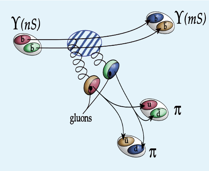
Figure 1: Left frame: Zweig-suppressed diagram for the transition $\Upsilon(nS)\to\Upsilon(mS)\pi\pi$ with $m<n$, which forms the basis of the QCD estimates of the decay rates and distributions in heavy quarkonia dipionic transitions. Right frame: The dipion invariant mass spectrum $M_{\pi\pi}$ measured in the decay $\Upsilon(4S)\to\Upsilon(1S)\pi\pi$ by the Belle collaboration together with a theoretical curve based essentially on the diagram shown in the left frame. (From  [16].)

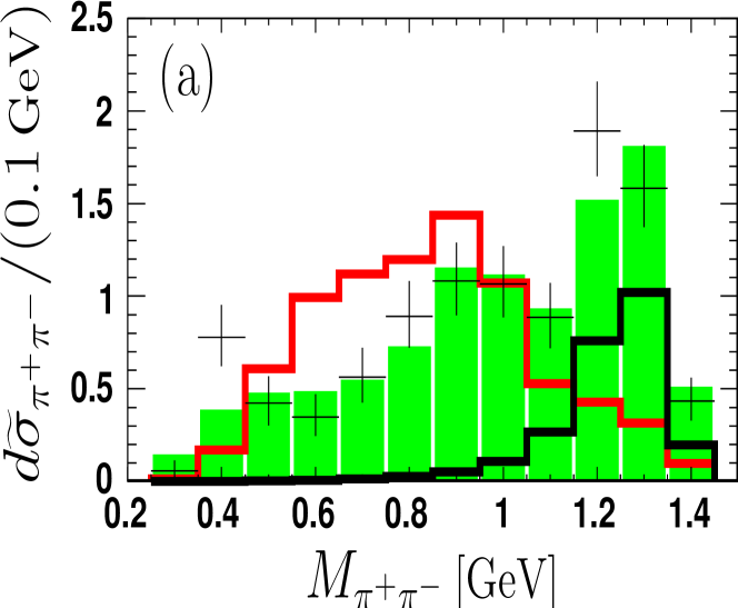
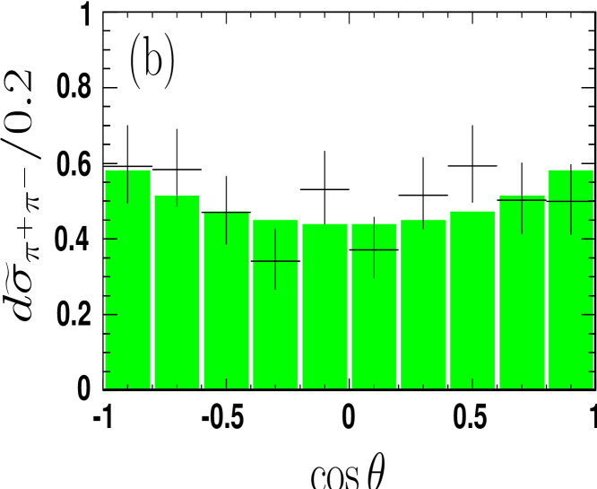
Figure 2: Fit results of the $M_{\pi^{+}\pi^{-}}$ distribution (a) and the $\cos\theta$ distribution (b) for $e^{+}e^{-}\to Y_{b}\to\Upsilon(1S)\pi^{+}\pi^{-}$, normalized by the measured cross section by Belle [12]. The histograms represent theoretical fit results based on the tetraquarks hypothesis, while the crosses are the Belle data. The solid curves in (a) show purely resonant contributions from the $f_{0}(980)$ and $f_{2}(1270)$. (From  [18].)

Not only are the cross sections for $e^{+}e^{-}\to\Upsilon(nS)\pi^{+}\pi^{-}$ ($n=1,2,3$) near the $\Upsilon(5S)$ anomalously large by at least two orders of magnitude, the same holds for the production of the P-wave spin-singlet bottomonia states $h_{b}(mP)$ ($m=1,2$), for which the production cross sections for $e^{+}e^{-}\to h_{b}(1P)\pi^{+}\pi^{-}$ and $e^{+}e^{-}\to h_{b}(2P)\pi^{+}\pi^{-}$ are also anomalously large [4]. The ratios of the production cross-sections in the indicated final states relative to that for the $e^{+}e^{-}\to\Upsilon(2S)\pi^{+}\pi^{-}$ production are as follows [4]:

$$\tilde{\sigma}[\Upsilon(1S)\pi^{+}\pi^{-}] = 0.638\pm 0.065^{+0.037}_{-0.056}$$

$$\tilde{\sigma}[\Upsilon(3S)\pi^{+}\pi^{-}] = 0.517\pm 0.082\pm 0.070$$

$$\tilde{\sigma}[h_{b}(1P)\pi^{+}\pi^{-}] = 0.407\pm 0.07^{+0.043}_{-0.076}$$

$$\tilde{\sigma}[h_{b}(2P)\pi^{+}\pi^{-}] = 0.78\pm 0.09^{+0.22}_{-0.10}$$ (1)

We have already commented on the anomalous production cross sections in the $\Upsilon(ns)\pi^{+}\pi^{-}$ modes near the $\Upsilon(5S)$ region. The ratios given in the last two equations above for the $h_{b}(1P)\pi^{+}\pi^{-}$ and $h_{b}(2P)\pi^{+}\pi^{-}$ are found to be of order unity, a feature which violates theoretical expectations as the processes $\Upsilon(5S)\to h_{b}(mP)\pi^{+}\pi^{-}$ involve heavy quark spin-flip, which are suppressed by $1/m_{b}$ in the amplitude. It is obvious that the production mechanisms of all five processes involving $\Upsilon(nS)\pi^{+}\pi^{-}$ ($n=1,2,3$) and $h_{b}(mP)\pi^{+}\pi^{-}$ ($m=1,2$) are exotic. In particular, the true mechanisms at work avoid the Zweig-suppression seen in similar dipionic transitions and evade power suppression due to the spin-flip transitions for the $h_{b}(mP)\pi^{+}\pi^{-}$ case. It is worth recalling that no excess of the kind seen in the Belle measurements near the $\Upsilon(5S)$ [12, 13, 4] is seen by them or any other experiment either at energies below or above the $\Upsilon(5S)$ region. Any plausible theoretical explanation must account for all these features.

These measurements have invoked a number of theoretical ideas. Particularly interesting is the suggestion by Bondar et al. [19], in which the resonances $Z_{b}(10610)$ and $Z_{b}(10650)$ are assumed mostly of a ’molecular’ type due to their respective proximity with the $B^{*}\bar{B}$ and $B^{*}\bar{B}^{*}$ thresholds. Thus, the internal dynamics of the states $Z_{b}(10610)$ and $Z_{b}(10650)$ is dominated by the coupling to meson pairs $B^{*}\bar{B}-B\bar{B}^{*}$ and $B^{*}\bar{B}^{*}$, respectively. In particular, the $b\bar{b}$ pair within the $Z_{b}(10610)$ and $Z_{b}(10650)$ is an equal mixture of a spin-triplet and spin-singlet with the relative phase orthogonal between the two resonances, i.e.,

$$|Z_{b}(10610)\rangle = \frac{1}{\sqrt{2}}\left(0^{-}_{b\bar{b}}\otimes 1^{-}_{\bar{Q}q}-1^{-}_{b\bar{b}}\otimes 0^{-}_{\bar{Q}q}\right)~{},$$

$$|Z_{b}(10650)\rangle = \frac{1}{\sqrt{2}}\left(0^{-}_{b\bar{b}}\otimes 1^{-}_{\bar{Q}q}+1^{-}_{b\bar{b}}\otimes 0^{-}_{\bar{Q}q}\right)~{}.$$ (2)

Here $0^{-}$ and $1^{-}$ stand for the para- and ortho-states with negative parity. The assignments (2) would predict that the mass difference $M[Z_{b}(10650)]-M[Z_{b}(10610)]$ should be equal to that between the $B$ and $B^{*}$ masses. The observed mass difference of 46 MeV [4] is in neat agreement with this argument. The spin-structure in (2) also suggests that the resonances $Z_{b}(10610)$ and $Z_{b}(10650)$ have the same decay width. This again is in agreement within measurement errors with the Belle data [4]: $\Gamma[Z_{b}(10610)]=15.6\pm 2.5$ MeV and $\Gamma[Z_{b}(10650)]=14.4\pm 3.2$ MeV. The maximal ortho-para mixing of the heavy quarks in the $Z_{b}(10610)$ and $Z_{b}(10650)$ resonances described by Eq. (2) also implies couplings of comparable strengths to channels with states of ortho- and para-bottomonium, leading to the following couplings of these resonances to the channels $\Upsilon(nS)\pi^{\pm}$ and $h_{b}(mP)\pi^{\pm}$[19]:

$$C_{h}\,\,E_{\pi}\,\vec{\Upsilon}(nS)\cdot(\vec{Z}_{b}(10610)-\vec{Z}_{b}(10650))~{},~{}~{}~{}~{}C_{\Upsilon}(\vec{p}_{\pi}\,\,\times\vec{h}_{b})\cdot(\vec{Z}_{b}(10610)+\vec{Z}_{b}(10650))~{},$$ (3)

where $\vec{Z}_{b}(10610)$, $\vec{Z}_{b}(10650)$ and $\vec{h}_{b}$ denote the polarization vectors of the corresponding spin-1 states, and $E_{\pi}$ and $\vec{p}_{\pi}$ are the pion energy and its three-momentum, respectively; $C_{h}$ and $C_{\Upsilon}$ are a priori unknown coupling constants to be determined by data. The amplitudes described by Eq. (3) applied to the decays $\Upsilon(5S)\to\Upsilon(nS)\pi^{+}\pi^{-}$ and $\Upsilon(5S)\to h_{b}(mS)\pi^{+}\pi^{-}$ yield the right pattern of destructive and constructive interferences seen in the Dalitz distributions of these processes [4]. All of these arguments are plausible. Further variations on the molecular theme and predictions can be seen in  [20, 21, 22, 23].

However, the structure suggested in Eq. (2) is a postulate not yet seen in decays other than those of the $\Upsilon(5S)$. A particular case in point are the decays of the $\Upsilon(6S)$, where the available phase space for the decays $\Upsilon(6S)\to\Upsilon(nS)\pi^{+}\pi^{-}$ and $\Upsilon(6S)\to h_{b}(mP)\pi^{+}\pi^{-}$ are much larger. Hence, the implications of Eqs. (2) and (3) should be, at least qualitatively, very similar to those discussed in the context of the Belle data from the $\Upsilon(5S)$ region. This remains to be tested. In addition, there are also some specific features of the Belle data which do not go hand-in-hand with the usual understanding of a hadronic molecule, the closest example of which is the Deuteron. The masses of the $Z_{b}(10610)$ and $Z_{b}(10650)$ are above the respective thresholds. The Deuteron mass, on the other hand, lies below the threshold by about 2.2 MeV. Also, the decay widths of the $Z_{b}(10610)$ and $Z_{b}(10650)$ are not particularly small, as one would expect for a hadron molecule. On the contrary, their decay widths are similar in order of magnitude as that of the $\Upsilon(5S)$. This is also curious as the other ’hadronic molecule’ discussed at length in a similar context, namely the $X(3872)$, has a much smaller (by at least an order of magnitude) decay width, with the current 90% C.L. limit being $\Gamma[X(3872)]<1.2$ MeV [24].

In the rest of this writeup, I will take the point of view that all the five anomalous processes measured by Belle at energies near the $\Upsilon(5S)$ mass [12, 13, 4] have very little to do with the $\Upsilon(5S)$ decays. Following  [17, 18, 25], I will argue here that the final states $\Upsilon(nS)\pi^{+}\pi^{-}$ and $h_{b}(mP)\pi^{+}\pi^{-}$ are the decay products of the $J^{PC}=1^{--}$ tetraquark $Y_{b}(10890)$, which lies in mass tantalizingly close to the $\Upsilon(5S)$ mass. More precise experiments are needed to tell the two apart than is the case currently. In the context of the $\Upsilon(nS)\pi^{+}\pi^{-}$ final states, this was suggested in [17, 18, 25] and the dynamical model was shown to be consistent with the observed cross sections. Also, the measured dipion invariant mass distributions show the predicted scalar-and tensor-meson resonant structure. Moreover, in the tetraquark context, it is easier to understand why the production cross sections for $e^{+}e^{-}\to Y_{b}(10890)\to\Upsilon(nS)\pi^{+}\pi^{-}$, which involves a ${}^{3}P\to{}^{3}S$ transition, and for $e^{+}e^{-}\to Y_{b}(10890)\to h_{b}(mS)\pi^{+}\pi^{-}$, which involves a ${}^{3}P\to{}^{1}P$ transition, are comparable to each other. Detailed distributions, including the resonant $Z_{b}(10610)$ and $Z_{b}(10650)$ effects are still being worked out in the tetraquark picture.

3 Spectrum of bottom diquark-antidiquark states

Much of the discussion of the tetraquark states involves the concept of diquarks (and anti-diquarks) as effective degrees of freedom, which will be used here to calculate the mass spectra, production and decay of the tetraquark states. In particular, four-quark configurations in the tetraquarks are assumed not to play a dominant role. Following this, the mass spectrum of tetraquarks $[bq][\overline{bq^{\prime}]}$ with $q=u$, $d$, $s$ and $c$ can be calculated using a Hamiltonian [26]

$$H=2m_{\it Q}+H_{SS}^{(\it Q\it Q)}+H_{SS}^{(\it Q\bar{\it Q}\mathcal{)}}+H_{SL}+H_{LL},$$ (4)

where:

$$H_{SS}^{(\it Q\it Q)} = 2(\mathcal{K}_{bq})_{\bar{3}}[(\mathbf{S}_{b}\cdot\mathbf{S}_{q})+(\mathbf{S}_{\bar{b}}\cdot\mathbf{S}_{\bar{q}})],$$

$$H_{SS}^{(\it Q\bar{\it Q}\mathcal{)}} = 2(\mathcal{K}_{b\bar{q}})(\mathbf{S}_{b}\cdot\mathbf{S}_{\bar{q}}+\mathbf{S}_{\bar{b}}\cdot\mathbf{S}_{q})+2\mathcal{K}_{b\bar{b}}(\mathbf{S}_{b}\cdot\mathbf{S}_{\bar{b}})+2\mathcal{K}_{q\bar{q}}(\mathbf{S}_{q}\cdot\mathbf{S}_{\bar{q}}),$$

$$H_{SL} = 2A_{\it Q}(\mathbf{S}_{\mathcal{Q}}\cdot\mathbf{L}+\mathbf{S}_{\mathcal{\bar{Q}}}\cdot\mathbf{L}),$$

$$H_{LL} = B_{\it Q}\frac{L_{\it Q\bar{\it Q}}(L_{\it Q\bar{\it Q}}+1)}{2}~{}.$$ (5)

All diquarks, denoted here by $\it Q$ are assumed to be in the color triplet $(\bar{3})$, as the diquarks in the $(6)$ representation do not show binding [27]. Here $m_{\it Q}$ is the constituent mass of the diquark $[bq]$, $(\mathcal{K}_{bq})_{\bar{3}}$ is the spin-spin interaction between the quarks inside the diquarks, $\mathcal{K}_{b\bar{q}}$ are the couplings ranging outside the diquark shells, $A_{\it Q}$ is the spin-orbit coupling of diquark and $B_{\it Q}$ corresponds to the contribution of the total angular momentum of the diquark-antidiquark system to its mass. The overall factor of $2$ is used customarily in the literature. As the isospin-breaking effects are estimated to be of order 5 - 8 MeV for the tetraquarks $[bq][\bar{b}\bar{q}]$ [25, 26], they are neglected in the mass estimates discussed below.

The parameters involved in the above Hamiltonian (5) can be obtained from the known meson and baryon masses by resorting to the constituent quark model [29]

$$H=\sum\limits_{i}m_{i}+\sum\limits_{i<j}2\mathcal{K}_{ij}(\mathbf{S}_{i}\cdot\mathbf{S}_{j}),$$ (6)

where the sum runs over the hadron constituents. The coefficient $\mathcal{K}_{ij}$ depends on the flavour of the constituents $i$, $j$ and on the particular colour state of the pair. The constituent quark masses and the couplings $\mathcal{K}_{ij}$ for the colour singlet and anti-triplet states are given in  [25]. To calculate the spin-spin interaction of the $\it Q\bar{\it Q}$ states explicitly, one uses the non-relativistic notation [28] $\left|S_{\it Q},S_{\bar{\it Q}};~{}J\right\rangle$, where $S_{\it Q}$ and $S_{\bar{\it Q}}$ are the spin of diquark and antidiquark, respectively, and $J$ is the total angular momentum. These states are then defined in terms of the direct product of the $2\times 2$ matrices in spinor space, $\Gamma^{\alpha}$, which can be written in terms of the Pauli matrices as:

$$\Gamma^{0}=\frac{\sigma_{2}}{\sqrt{2}};~{}\Gamma^{i}=\frac{1}{\sqrt{2}}\sigma_{2}\sigma_{i}~{},$$ (7)

which then lead to the definition such as $\left|0_{\it Q},0_{\bar{\it Q}};~{}0_{J}\right\rangle=\frac{1}{2}\left(\sigma_{2}\right)\otimes\left(\sigma_{2}\right)$. Others can be seen in [25].

The next step is the diagonalization of the Hamiltonian (4) using the basis of states with definite diquark and antidiquark spin and total angular momentum., There are two different possibilities [28]: Lowest lying $[bq][\bar{b}\bar{q}]$ states $\left(L_{\it Q\bar{\it Q}}=0\right)$ and higher mass $[bq][\bar{b}\bar{q}]$ states $\left(L_{\it Q\bar{\it Q}}=1\right)$. The $[bq][\bar{b}\bar{q}]$ states $\left(L_{\it Q\bar{\it Q}}=0\right)$ can be classified in terms of the six possible states involving the good (spin-0) and bad (spin-1) diquarks (here, $P$ is the parity and $C$ the charge conjugation)

i. Two states with $J^{PC}=0^{++}$:

$$\left|0^{++}\right\rangle = \left|0_{\it Q},0_{\bar{\it Q}};~{}0_{J}\right\rangle;$$

$$\left|0^{++\prime}\right\rangle = \left|1_{\it Q},1_{\bar{\it Q}};~{}0_{J}\right\rangle.$$ (8)

ii. Three states with $J=1$:

$$\left|1^{++}\right\rangle = \frac{1}{\sqrt{2}}\left(\left|0_{\it Q},1_{\bar{\it Q}};~{}1_{J}\right\rangle+\left|1_{\it Q},0_{\bar{\it Q}};~{}1_{J}\right\rangle\right);$$

$$\left|1^{+-}\right\rangle = \frac{1}{\sqrt{2}}\left(\left|0_{\it Q},1_{\bar{\it Q}};~{}1_{J}\right\rangle-\left|1_{\it Q},0_{\bar{\it Q}};~{}1_{J}\right\rangle\right);$$

$$\left|1^{+-\prime}\right\rangle = \left|1_{\it Q},1_{\bar{\it Q}};~{}1_{J}\right\rangle.$$ (9)

All these states have positive parity as both the good and bad diquarks have positive parity and $L_{\it Q\bar{\it Q}}=0$. The difference is in the charge conjugation quantum number, the state $\left|1^{++}\right\rangle$ is even under charge conjugation, whereas $\left|1^{+-}\right\rangle$ and $\left|1^{+-\prime}\right\rangle$ are odd.

iii. One state with $J^{PC}=2^{++}$:

$$\left|2^{++}\right\rangle=\left|1_{\it Q},1_{\bar{\it Q}};~{}2_{J}\right\rangle.$$ (10)

Keeping in view that for $L_{\it Q\bar{\it Q}}=0$ there is no spin-orbit and purely orbital term, the Hamiltonian (4) takes the form

$$H = 2m_{\it Q}+2(\mathcal{K}_{bq})_{\bar{3}}[(\mathbf{S}_{b}\cdot\mathbf{S}_{q})+(\mathbf{S}_{\bar{b}}\cdot\mathbf{S}_{\bar{q}})]+2\mathcal{K}_{q\bar{q}}(\mathbf{S}_{q}\cdot\mathbf{S}_{\bar{q}})$$ (11)

$$+2(\mathcal{K}_{b\bar{q}})(\mathbf{S}_{b}\cdot\mathbf{S}_{\bar{q}}+\mathbf{S}_{\bar{b}}\cdot\mathbf{S}_{q})+2\mathcal{K}_{b\bar{b}}(\mathbf{S}_{b}\cdot\mathbf{S}_{\bar{b}}).$$

The diagonalisation of the Hamiltonian (11) with the states defined above gives the eigenvalues which are needed to estimate the masses of these states. For the $1^{++}$ and $2^{++}$ states the Hamiltonian is diagonal with the eigenvalues [28]

$$M\left(1^{++}\right) = 2m_{\it Q}-(\mathcal{K}_{bq})_{\bar{3}}+\frac{1}{2}\mathcal{K}_{q\bar{q}}-\mathcal{K}_{b\bar{q}}+\frac{1}{2}\mathcal{K}_{b\bar{b}},$$ (12)

$$M\left(2^{++}\right) = 2m_{[bq]}+(\mathcal{K}_{bq})_{\bar{3}}+\frac{1}{2}\mathcal{K}_{q\bar{q}}+\mathcal{K}_{b\bar{q}}+\frac{1}{2}\mathcal{K}_{b\bar{b}}.$$ (13)

Mass of the constituent diquark can be estimated in one of two ways: We take the Belle data [12] as input and identify the $Y_{b}(10890)$ with the lightest of the $1^{--}$ states, $Y_{[bq]}$, yielding a diquark mass $m_{[bq]}=5.251\;\textnormal{GeV}$. This procedure is analogous to what was done in [28], in which the mass of the diquark $[cq]$ was fixed by using the mass of $X(3872)$ as input, yielding $m_{[cq]}=1.933$ GeV. Instead, if we use this determination of $m_{[cq]}$ and use the formula $m_{[bq]}=m_{[cq]}+\left(m_{b}-m_{c}\right)$, which has the virtue that the mass difference $m_{c}-m_{b}$ is well determined, we get $m_{[bq]}=5.267\;\textnormal{GeV}$, yielding a difference of $16\;\textnormal{MeV}$. This can be taken as an estimate of the theoretical error on $m_{[bq]}$, which then yields an uncertainty of about 30 MeV in the estimates of the tetraquark masses from this source alone. For the corresponding $0^{++}$ and $1^{+-}$ tetraquark states, there are two states each, and hence the Hamiltonian is not diagonal. After diagonalising the $2\times 2$ matrices, the masses of these states are obtained.

We now discuss orbital excitations with $L_{\it Q\bar{\it Q}}=1$ having both good and bad diquarks. Concentrating on the $1^{--}$ multiplet, we recall that there are eight tetraquark states $[bq][\bar{b}\bar{q}]$ ($q=u,d$), and the lightest isospin doublet is:

$$M_{Y_{[bq]}}^{(1)}\left(S_{\it Q}=0,~{}S_{\bar{\it Q}}=0,~{}S_{\it Q\bar{\it Q}}=0,~{}L_{\it Q\bar{\it Q}}=1\right)=m_{\left[bq\right]}+\lambda_{1}+B_{\mathcal{\it Q}},$$ (14)

and the next in mass is: $M_{Y_{[bq]}}^{(2)}\left(S_{\it Q}=1,~{}S_{\bar{\it Q}}=0,~{}S_{\it Q\bar{\it Q}}=1,~{}L_{\it Q\bar{\it Q}}=1\right)=2m_{\left[bq\right]}+\Delta+\lambda_{2}-2A_{\it Q}+B_{\it Q}$, and so on. Values of $\lambda_{i}(i=1,2,3)$, $A_{\it Q}$ and $B_{\it Q}$ are estimated in [25]. We identify the state $Y_{b}(10890)$ with $M_{Y_{[bq]}}^{(1)}$ (in fact there are two of them, which differ in mass from each other by about 5 - 8 MeV, including isospin-breaking). This does not fix the quantity $\Delta$, which is the mass difference of the good and the bad diquarks, i.e. $\Delta=m_{\it Q}\left(S_{\it Q}=1\right)-m_{\it Q}\left(S_{\it Q}=0\right)$. Following Jaffe and Wilczek [27], the value of $\Delta$ for diquark $[bq]$ is estimated as $\Delta=202$ MeV for $q=u$, $d$, $s$ and $c$ quarks. This is another source of potential uncertainty in estimating the tetraquark masses. The mass spectrum for the tetraquark states $[bq][\bar{b}\bar{q}]$ for $q=u,d$ with $J^{PC}=0^{++},1^{++},1^{+-},1^{--}$ and $2^{++}$ states is plotted in Fig. 3 in the isospin-symmetry limit. It is difficult to quote a theoretical error on the masses shown, with $\pm 50$ MeV presumably a good guess. Other estimates of the tetraquark mass spectra in the charm and bottom quark sectors can be seen in  [31, 32, 33].

3.1 Estimates of the charged $J^{P}=1^{+}$ tetraquark states

In the tetraquark picture, one also anticipates a large number of charged states whose mass spectrum can be calculated in an analogous fashion as for their neutral counterparts just discussed. We would like to propose that the two charged $J^{P}=1^{+}$ states $Z_{b}(10610)$ and $Z_{b}(10650)$ observed recently by the Belle Collaboration [3], and interpreted by them as the charged bottomonium states produced in the process $\Upsilon(5S)\to Z^{\pm}_{b}(10610)+\pi^{\mp}$ and $\Upsilon(5S)\to Z^{\pm}_{b}(10650)+\pi^{\mp}$, are indeed charged tetraquark states with the quark content $Z_{b}^{+}=[bu][\bar{b}\bar{d}]$ for the positively charged state (its charge conjugate being $Z_{b}^{-}=[\bar{b}\bar{u}][bd]$). For the present discussion, they are produced in the decays of the $J^{PC}=1^{--}$ tetraquark $Y_{b}(10890)$. According to this interpretation, the decay chains involve $Y_{b}(10890)\to((Z^{\pm}_{b}(10610),Z^{\pm}_{b}(10650)+\pi^{\mp}\to\Upsilon(ns)\pi^{+}\pi^{-}$. A detailed dynamical model is under development with the aim of understanding the decay distributions in the kinematic variables available in these decays.

We have estimated the masses of the isospin partners of $Z_{b}(10610)$ and $Z_{b}(10650)$, the two neutral $J=1$ tetraquark states, denoted as $|1^{+-}\rangle$ and $|1^{+-\prime}\rangle$. The $2\times 2$ non-diagonal mass matrix for the neutral $J^{PC}=1^{+-}$ states was, however, calculated numerically for $\Delta=0$. If we ignore the isospin-breaking effects in the tetraquark masses, which are small, then the charged counterparts have the masses $M[Z_{b}(10610)]=10.386$ GeV and $M[Z_{b}(10650)]=10.527$ GeV, given in Fig. 3. As $Z_{b}(10610)$ involves one good and one bad diquark and $Z_{b}(10650)$ involves two bad diquarks, including the $\Delta$-dependent term, the non-diagonal $2\times 2$ mass matrix gets modified to the following form

$$M(1^{+-}) = 2m_{\it Q}+\frac{3}{2}\Delta-\frac{\kappa_{q\bar{q}}+\kappa_{b\bar{b}}}{2}+\left(\begin{array}[]{cc}-\frac{\Delta}{2}-(\kappa_{bq})_{\bar{3}}+\kappa_{b\bar{q}}&\kappa_{q\bar{q}}-\kappa_{b\bar{b}}\\ \kappa_{q\bar{q}}-\kappa_{b\bar{b}}&\frac{\Delta}{2}+(\kappa_{bq})_{\bar{3}}-\kappa_{b\bar{q}}\end{array}\right)~{}.$$ (17)

The two eigenvalues can be written as $E=\pm\sqrt{x^{2}+y^{2}}$, with $x=\frac{\Delta}{2}+(\kappa_{bq})_{\bar{3}}-\kappa_{b\bar{q}}$ and $y=\kappa_{q\bar{q}}-\kappa_{b\bar{b}}$, yielding

$$M[Z_{b}(10650)]=2m_{\it Q}+\frac{3}{2}\Delta-\frac{\kappa_{q\bar{q}}+\kappa_{b\bar{b}}}{2}+\sqrt{(\frac{\Delta}{2}+(\kappa_{bq})_{\bar{3}}-\kappa_{b\bar{q}})^{2}+(\kappa_{q\bar{q}}-\kappa_{b\bar{b}})^{2}}~{},$$ (18)

$$M[Z_{b}(10610)]=2m_{\it Q}+\frac{3}{2}\Delta-\frac{\kappa_{q\bar{q}}+\kappa_{b\bar{b}}}{2}-\sqrt{(\frac{\Delta}{2}+(\kappa_{bq})_{\bar{3}}-\kappa_{b\bar{q}})^{2}+(\kappa_{q\bar{q}}-\kappa_{b\bar{b}})^{2}}~{}.$$ (19)

Using the default values of the parameters [25]

$$m_{\it Q}=5.251~{}{\rm GeV},\;(\kappa_{q\bar{q}})_{0}=318~{}{\rm MeV},\;\;(\kappa_{b\bar{b}})_{0}=36~{}{\rm MeV},\;\;(\kappa_{b\bar{q}})_{0}=23~{}{\rm MeV},\;\;(\kappa_{bq})_{3}=6~{}{\rm MeV}$$

we have now the following predictions for the two charged tetraquark masses

$$M[Z_{b}(10610)]=10.637~{}{\rm GeV};\;\;\;M[Z_{b}(10650)]=10.884~{}{\rm GeV},\;\;\;{\rm with}\;\;\Delta=202~{}{\rm MeV}~{}.$$ (21)

These estimates are to be compared with the masses of the $J^{P}=1^{+}$ states $Z_{b}(10610)$ and $Z_{b}(10650)$ reported by the Belle Collaboration [3] $M[Z_{b}(10610)]=(10608\pm 2.0)$ MeV and $M[Z_{b}(10650)]=(10653.2\pm 1.5)$ MeV. They are in the right ball-park, but miss the measurements by approximately 30 MeV and 230 MeV, respectively. More importantly, the mass difference between the two states has been measured precisely [3] $M[Z_{b}(10650)]-M[Z_{b}(10610)]\simeq 45$ MeV. The expression for this mass difference using the Hamiltonian (5) is:

$$M[Z_{b}(10650)]-M[Z_{b}(10610)]=2\sqrt{(\frac{\Delta}{2}+(\kappa_{bq})_{\bar{3}}-\kappa_{b\bar{q}})^{2}+(\kappa_{q\bar{q}}-\kappa_{b\bar{b}})^{2}}~{}.$$ (22)

The smallest value for the mass difference (140 MeV) is obtained for $\Delta=0$, which goes up to 247 MeV for $\Delta=202{\rm MeV}$. Both are larger than the measurements. Thus, the Belle data suggests that the Hamiltonian used here has to be augmented with an additional contribution. As the masses of the observed states $Z_{b}(10610)$ and $Z_{b}(10650)$ are rather close to the thresholds $M(B)+M(B^{*})$ and $2M(B^{*})$, respectively, this suggests that the threshold effects may impact on the masses and mass differences presented here.

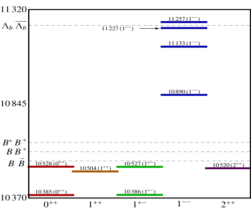
Figure 3: Tetraquark mass spectrum with the valence quark content $[bq][\bar{b}\bar{q}]$ with $q=u,d$, assuming isospin symmetry. The value 10890 is an input for the lowest $J^{PC}=1^{--}$ tetraquark state $Y_{[bq]}$. All masses are given in MeV. (From [25].)

4 Tetraquark-based analysis of the processes $e^{+}e^{-}\to\Upsilon(1S)(\pi^{+}\pi^{-},K^{+}K^{-},\eta\pi^{0})$

The cross sections and final state distributions for the processes $e^{+}e^{-}\to\Upsilon(1S)(\pi^{+}\pi^{-},K^{+}K^{-},\eta\pi^{0})$ near the $\Upsilon(5S)$ have been presented in the tetraquark picture in [18] improving the results on the process $e^{+}e^{-}\to\Upsilon(1S)\pi^{+}\pi$ published earlier [17]. The distributions for the process $e^{+}e^{-}\to\Upsilon(2S)\pi^{+}\pi$ calculated in [17] had a computational error, which has been corrected in the meanwhile (see the Erratum in  [17]). These analyses are briefly reviewed in this section. Concentrating on the processes $e^{+}e^{-}\to\Upsilon(1S)(\pi^{+}\pi^{-},K^{+}K^{-},\eta\pi^{0})$, there are essentially three important parts of the amplitude to be calculated consisting of the following:

(i) Production mechanism of the $J^{PC}=1^{--}$ vector tetraquarks in $e^{+}e^{-}$ annihilation. To that end, we derive the equivalent of the Van-Royen-Weiskopf formula for the leptonic decay widths of the tetraquark states $Y_{[bu]}$ and $Y_{[bd]}$ made up of a diquark and antidiquark, based on the diagram shown in Fig. 4 (left-hand frame).

$$\Gamma(Y_{[bu/bd]}\to e^{+}e^{-})=\frac{24\alpha^{2}|Q_{[bu/bd]}|^{2}}{m_{Y_{b}}^{4}}\,\kappa^{2}\left|R^{(1)}_{11}(0)\right|^{2}~{}.$$ (23)

Here, $Q_{[bu]}=1/3$ and $Q_{[bd]}=-2/3$ are the electric charges of the constituent diquarks of the $Y_{[bu]}$ and $Y_{[bd]}$, $\alpha$ is the fine-structure constant, the parameter $\kappa$ takes into account differing sizes of the tetraquarks compared to the standard bottomonia, with $\kappa<1$ anticipated, and $|R^{(1)}_{11}(0)|^{2}=2.067$ GeV⁵ [34] is the square of the derivative of the radial wave function for $\chi_{b}(1P)$ taken at the origin. Hence, the leptonic widths of the tetraquark states are estimated as

$$\Gamma(Y_{[bd]}\to e^{+}e^{-})=4\,\Gamma(Y_{[bu]}\to e^{+}e^{-})\approx 83\,\kappa^{2}\ {\rm eV}\,,$$ (24)

which are substantially smaller than the leptonic width of the $\Upsilon(5S)$ [5]. This is the reason why the states $Y_{[bd]}$ and $Y_{[bu]}$ are not easily discernible in the $R_{b}$-scan. Between the two, $Y_{[bd]}$ production dominates and should be searched for in dedicated experiments. However, as the decays $\Upsilon(5S)\to\Upsilon(nS)\pi^{+}\pi^{-}$ are Zweig-suppressed in the conventional Quarkonia descriptions, and hence have small branching ratios, the signal-to-background is much better for the discovery of the $Y_{b}(10890)$ in the states $\Upsilon(nS)\pi^{+}\pi^{-}$. These, in fact, are the discovery channels of the $Y_{b}(10890)$ [13].

(ii) The decay amplitudes for $Y_{b}(10890)\to\Upsilon(1S)(\pi^{+}\pi^{-},K^{+}K^{-},\eta\pi^{0})$ have non-resonant (continuum) contributions, as depicted in Fig. 4 (middle frame). They are parametrised in terms of two a priori unknown constants $A$ and $B$ , following [14]:

$${\cal M}_{0}^{1C} = \frac{2A}{f_{P}f_{P^{\prime}}}(k_{1}\cdot k_{2})+\frac{B}{f_{P}f_{P^{\prime}}}\frac{3(q^{0})^{2}k_{1}^{0}k_{2}^{0}-|\mathbf{q}|^{2}|\mathbf{k}|^{2}}{3s}\,,$$

$${\cal M}_{0}^{2C} = -\frac{B}{f_{P}f_{P^{\prime}}}\frac{|\mathbf{q}|^{2}|\mathbf{k}|^{2}}{s}\,,$$ (25)

where the subscript $0$ denotes the $I=0$ part of the amplitudes, the superscripts 1C and 2C correspond to the $S$- and $D$-wave continuum contributions, respectively, $f_{P^{(\prime)}}$ is the decay constant of $P^{(\prime)}$, and $|\mathbf{q}|$, $k_{1}^{0}$ and $k_{2}^{0}$ are the magnitude of the three momentum of $Y_{b}$ and the energies of $P$ and $P^{\prime}$ in the $PP^{\prime}$ rest frame, respectively. Using SU(3) symmetry results in the relations involving the various $I=0$ and $I=1$ amplitudes: ${\cal M}_{0}^{1C,2C}(\Upsilon(1S)K^{+}K^{-})=(\sqrt{3}/2)\,{\cal M}_{0}^{1C,2C}(\Upsilon(1S)\pi^{+}\pi^{-})$, ${\cal M}_{1}^{1C,2C}(\Upsilon(1S)K^{+}K^{-})={\cal M}_{0}^{1C,2C}(\Upsilon(1S)K^{+}K^{-})$ and ${\cal M}_{1}^{1C,2C}(\Upsilon(1S)\eta\pi^{0})=\sqrt{2}\,{\cal M}_{1}^{1C,2C}(\Upsilon(1S)K^{+}K^{-})$. We note that, in general, there is a third constant also present in the non-resonant amplitudes, characterising the term depending on the polarisation of the $Y_{b}$. However, being suppressed by $1/m_{b}$, this is ignored.

(iii) The resonant contributions, shown in the right-hand frame of Fig. 4, are expressed by the Breit-Wigner formula:

$$\mathcal{M}^{R}_{I} = \frac{g_{RPP^{\prime}}\,g_{Y_{b}^{I}\Upsilon(1S)R}\,g_{e^{+}e^{-}Y_{b}^{0}}}{M_{PP^{\prime}}^{2}-m_{R}^{2}+i\,m_{R}\Gamma_{R}}\,e^{i\varphi_{R}},$$ (26)

where $I=0$ for $R=\sigma$, $f_{0}$ and $f_{2}$, and $I=1$ for $R=a_{0}^{0}$. The couplings for the scalar resonances $S$ are defined through the Lagrangian ${\cal L}=g_{SPP^{\prime}}(\partial_{\mu}P)(\partial^{\mu}P^{\prime})\,S+g_{Y_{b}\Upsilon(1S)S}\,Y_{b\mu}\Upsilon^{\mu}S$, while those for the $f_{2}$ are defined via ${\cal L}=2\hskip 0.85358ptg_{f_{2}PP^{\prime}}(\partial_{\mu}P)(\partial_{\nu}P^{\prime})f_{2}^{\mu\nu}+g_{Y_{b}\Upsilon(1S)f_{2}}Y_{b\mu}\Upsilon_{\nu}f_{2}^{\mu\nu}$. The couplings $g_{RPP^{\prime}}$ and $g_{Y_{b}^{I}\Upsilon(1S)R}$ have mass dimensions $-1$ and $1$, respectively. For the $\sigma$, $f_{0}$ and $a_{0}^{0}$, we adopt the Flatté model [35] and the details can be seen in [18].

With this input, a simultaneous fit to the binned $\Upsilon(1S)\pi^{+}\pi^{-}$ data for the $M_{\pi^{+}\pi^{-}}$ and $\cos\theta$ distributions measured by Belle at $\sqrt{s}=10.87$ GeV [12] were undertaken. Normalizing the distributions by the measured cross section: $d\widetilde{\sigma}_{\pi^{+}\pi^{-}}/dM_{\pi\pi}$ and $d\widetilde{\sigma}_{\pi^{+}\pi^{-}}/d\cos\theta$, where $\widetilde{\sigma}_{\pi^{+}\pi^{-}}\equiv\sigma_{\Upsilon(1S)\pi^{+}\pi^{-}}/\sigma_{\Upsilon(1S)\pi^{+}\pi^{-}}^{\rm{Belle}}$ with $\sigma_{\Upsilon(1S)\pi^{+}\pi^{-}}^{\rm{Belle}}=1.61\pm 0.16$ pb [12], the results are shown in Fig. 2 (histograms) and provide a good description of both the dipion mass spectrum and the angular distribution.

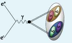
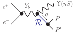
Figure 4: Left frame: Van Royen-Weiskopf Diagram for the production of a $J^{PC}=1^{--}$ tetraquark $Y_{b}$ with the quark content $[bu][\bar{b}\bar{u}]$ in the process $e^{+}e^{-}\to\gamma^{*}\to Y_{b}$. Middle frame: Continuum contribution in the process $e^{+}e^{-}\to Y_{b}\to\Upsilon(nS)PP^{\prime}$. Right frame: Resonance contribution in the process $e^{+}e^{-}\to Y_{b}\to\Upsilon(nS)PP^{\prime}$. (Figures based on [18].)

The normalized $M_{K^{+}K^{-}}$ and $M_{\eta\pi^{0}}$ distributions are shown in Fig. 5 (a) and Fig. 5 (b), respectively. In these figures, the dotted (solid) curves show the dimeson invariant mass spectra from the resonant (total) contribution. Since these spectra are dominated by the scalars $f_{0}+a_{0}^{0}$ and $a_{0}^{0}$, respectively, there is a strong correlation between the two cross sections. This is shown in Fig. 5 (c), where the normalized cross sections $\widetilde{\sigma}_{K^{+}K^{-}}$ and $\widetilde{\sigma}_{\eta\pi^{0}}$ are plotted resulting from the fits (dotted points) which all satisfy $\chi^{2}/{\rm d.o.f.}<1.6$ [18]. The current Belle measurement $\widetilde{\sigma}_{K^{+}K^{-}}=0.11^{+0.04}_{-0.03}$ [12] is shown as a shaded (green) band on this figure. The tetraquark model [18] is in agreement with the Belle measurement, and prediction $1.0\lesssim\widetilde{\sigma}_{\eta\pi^{0}}\lesssim 2.0$. will be further tested as and when the cross section $\widetilde{\sigma}_{\eta\pi^{0}}$ is measured. Another important test of the tetraquark model is [12]

$$\frac{\sigma_{\Upsilon(1S)K^{+}K^{-}}}{\sigma_{\Upsilon(1S)K^{0}\bar{K}^{0}}}=\frac{Q_{[bu]}^{2}}{Q_{[bd]}^{2}}=\frac{1}{4}\,.$$ (27)

This remains to be tested.

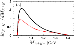
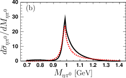
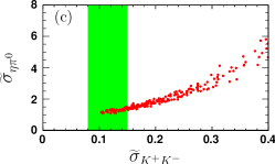
Figure 5: Predictions (a) of the $M_{K^{+}K^{-}}$ distribution for $e^{+}e^{-}\to Y_{b}\to\Upsilon(1S)K^{+}K^{-}$, (b) of the $M_{\eta\pi^{0}}$ distribution for $e^{+}e^{-}\to Y_{b}\to\Upsilon(1S)\eta\pi^{0}$ and (c) of the correlation between the cross sections of $\Upsilon(1S)K^{+}K^{-}$ and $\Upsilon(1S)\eta\pi^{0}$, normalized by the measured cross section for the $\Upsilon(1S)\pi^{+}\pi^{-}$ mode. In (a) and (b), the dotted (solid) curves show the dimeson invariant mass spectra from the resonant (total) contribution. In (c), the red dots represent predictions from the fit solutions satisfying $\chi^{2}/{\rm{d.o.f.}}<1.6$. The shaded (green) band shows the current Belle measurement $\widetilde{\sigma}_{K^{+}K^{-}}=0.11^{+0.04}_{-0.03}$ [12]. (From  [18].)

Finally, the corrected analysis [17] of the dipion invariant mass spectrum and the helicity angle distribution (in $\cos\theta$) for the process $Y_{b}(10890)\to\Upsilon(2S)\pi^{+}\pi^{-}$ are shown in Fig. 6, in which the normalization is given by the measured partial decay width $\Gamma[Y_{b}(10890)\to\Upsilon(2S)\pi^{+}\pi^{-}]=0.85\pm 0.7\pm 0.16$ MeV [13]. The dipion invariant mass spectrum is well accounted for also in this process ($\chi^{2}/{\rm d.o.f.}=12.6/7$), but not the the angular distribution $d\Gamma/d\cos\theta$. These distributions are being reevaluated taking into account the resonances $Z_{b}(10610)$ and $Z_{b}(10650)$.

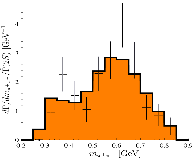
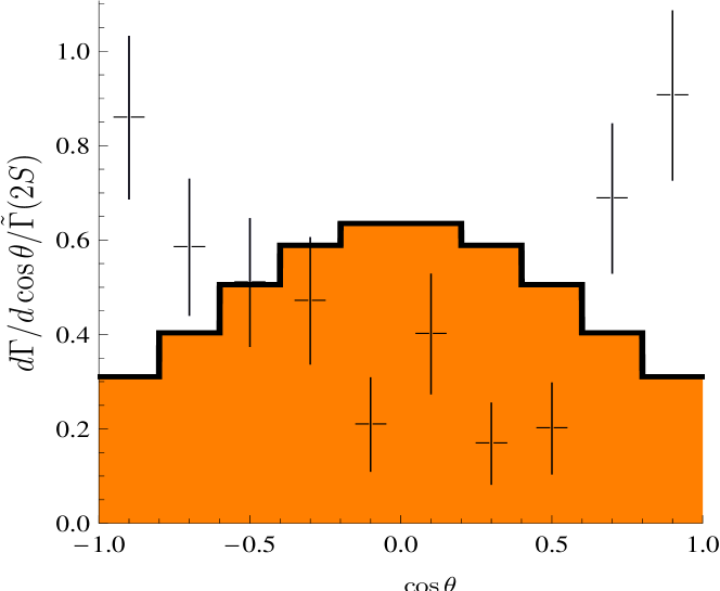
Figure 6: Dipion invariant mass $(m_{\pi\pi})$ distribution (left-handed frame) and the $\cos\theta$ distribution (right-handed frame) measured by the Belle collaboration for the final state $\Upsilon(2S)\pi^{+}\pi^{-}$  [12] and the corresponding theoretical distributions (histograms) based on the tetraquark interpretation of the $Y_{B}(10890)$. (From  [17].)

As a tentative summary of the tetraquark interpretation of the Belle data on $e^{+}e^{-}\to(\Upsilon(nS)\pi^{+}\pi^{-}$ and $e^{+}e^{-}\to h_{b}(mP)\pi^{+}\pi^{-}$ is that the existing analysis are encouraging and there exists a prima facie case of its validity. However, the missing contributions from the charged tetraquarks in the analysis of the $e^{+}e^{-}\to(\Upsilon(nS)\pi^{+}\pi^{-}$ data have to be incorporated and the fits of the $e^{+}e^{-}\to h_{b}(mP)\pi^{+}\pi^{-}$ data have to be undertaken to get a definitive answer.

I would like to thank Robert Fleischer and the organisers of the Beauty 2011 conference for a very exciting meeting in Amsterdam. I also thank Christian Hambrock, Satoshi Mishima and Wei Wang for their help in preparing this talk and helpful discussions.

References

[1]
S. L. Olsen,
Nucl. Phys. A 827, 53C (2009)
[arXiv:0901.2371 [hep-ex]];
A. Zupanc [for the Belle Collaboration],
arXiv:0910.3404 [hep-ex].
[2]
N. Brambilla et al.,
Eur. Phys. J. C 71, 1534 (2011).
[3]
I. Adachi et al. [Belle Collaboration],
arXiv:1105.4583 [hep-ex].
[4]
I. Adachi et al. [Belle Collaboration],
arXiv:1103.3419 [hep-ex].
[5]
C. Amsler et al. [Particle Data Group],
Phys. Lett. B 667, 1 (2008).
[6]
S. Godfrey, J. L. Rosner,
Phys. Rev. D66, 014012 (2002).
[arXiv:hep-ph/0205255 [hep-ph]].
[7]
J. P. Lees et al. [BABAR Collaboration],
arXiv:1102.4565 [hep-ex].
[8]
M. B. Voloshin,
Sov. J. Nucl. Phys. 43, 1011 (1986).
[9]
S. Godfrey,
J. Phys. Conf. Ser. 9, 123-126 (2005).
[hep-ph/0501083].
[10]
T. K. Pedlar et al. [CLEO Collaboration],
Phys. Rev. Lett. 107, 041803 (2011).
[11]
S. Dobbs et al. [ CLEO Collaboration ],
Phys. Rev. Lett. 101, 182003 (2008).
[arXiv:0805.4599 [hep-ex]].
[12]
K. F. Chen et al. [Belle Collaboration],
Phys. Rev. Lett. 100, 112001 (2008).
[13]
I. Adachi et al. [Belle Collaboration],
Phys. Rev. D82:091106(R) (2010).
[14]
L. S. Brown and R. N. Cahn,
Phys. Rev. Lett. 35, 1 (1975);
M. B. Voloshin,
JETP Lett. 21, 347 (1975)
[Pisma Zh. Eksp. Teor. Fiz. 21, 733 (1975)];
V. A. Novikov and M. A. Shifman,
Z. Phys. C 8, 43 (1981);
Y. P. Kuang and T. M. Yan,
Phys. Rev. D 24, 2874 (1981).
[15]
K. Gottfried,
Phys. Rev. Lett. 40, 598 (1978).
[16]
A. Sokolov et al. [Belle Collaboration],
Phys. Rev. D 79, 051103 (2009).
[17]
A. Ali, C. Hambrock and M. J. Aslam,
Phys. Rev. Lett. 104, 162001 (2010); 107, 049903 (E) (2011).
[18]
A. Ali, C. Hambrock and S. Mishima,
Phys. Rev. Lett. 106, 092002 (2011).
[19]
A. E. Bondar, A. Garmash, A. I. Milstein, R. Mizuk and M. B. Voloshin,
arXiv:1105.4473 [hep-ph].
[20]
M. B. Voloshin,
[arXiv:1105.5829 [hep-ph]].
[21]
M. Cleven, F. -K. Guo, C. Hanhart, U. -G. Meissner,
[arXiv:1107.0254 [hep-ph]].
[22]
Y. Yang, J. Ping, C. Deng, H. -S. Zong,
[arXiv:1105.5935 [hep-ph]].
[23]
Z. -F. Sun, J. He, X. Liu, Z. -G. Luo, S. -L. Zhu,
[arXiv:1106.2968 [hep-ph]].
[24]
S. -K. Choi, S. L. Olsen, K. Trabelsi,
[arXiv:1107.0163 [hep-ex]].
[25]
A. Ali, C. Hambrock, I. Ahmed and M. J. Aslam,
Phys. Lett. B 684, 28 (2010).
[26]
N. V. Drenska, R. Faccini and A. D. Polosa,
Phys. Lett. B 669, 160 (2008);
N. V. Drenska, R. Faccini and A. D. Polosa,
Phys. Rev. D 79, 077502 (2009).
[27]
R. L. Jaffe,
Phys. Rept. 409, 1 (2005)
[Nucl. Phys. Proc. Suppl. 142, 343 (2005)].
[28]
L. Maiani, F. Piccinini, A. D. Polosa and V. Riquer,
Phys. Rev. D 71, 014028 (2005)
[arXiv:hep-ph/0412098].
[29]
A. De Rujula, H. Georgi and S. L. Glashow,
Phys. Rev. D 12, 147 (1975).
[30]
R. L. Jaffe and F. Wilczek,
Phys. Rev. Lett. 91, 232003 (2003).
[31]
N. Drenska, R. Faccini, F. Piccinini, A. Polosa, F. Renga and C. Sabelli,
Riv. Nuovo Cim. 033, 633 (2010).
[32]
D. Ebert, R. N. Faustov and V. O. Galkin,
Mod. Phys. Lett. A 24, 567 (2009)
[arXiv:0812.3477 [hep-ph]].
[33]
Z. G. Wang,
Eur. Phys. J. C 67, 411 (2010)
[arXiv:0908.1266 [hep-ph]].
[34]
E. J. Eichten and C. Quigg,
Phys. Rev. D 52, 1726 (1995).