GM 2-4 - a signpost for low and intermediate mass star formation

Abstract

We present a multi-wavelength study of the region towards the GM 2-4 nebula and the nearby source IRAS 05373+2340. Our near-infrared H₂ 1-0 S(1) line observations reveal various shock-excited features which are part of several bipolar outflows. We identify candidates for the driving sources of the outflows from a comparison of the multi-waveband archival data-sets and SED modelling. The SED spectral slope ($\alpha^{IRAC}$) for all the protostars in the field was then compared with the visual extinction map. This comparison suggests that star formation is progressing from NE to SW across this region.

1 Introduction

Since 1998, the Byurakan observatory in Armenia has been engaged in surveys of nebular objects in dark molecular clouds and star formation regions. With its 2.6m telescope, imaging in narrow band filters and simultaneous searches of H$\alpha$ emission stars are being performed. New HH outflows and star forming regions have been found (see Movsessian et al., 2008, and references therein). An exploration of the region with GM 1-64 (RNO 53) (Gyulbudaghian & Maghakian, 1977; Cohen, 1980) and the GM 2-4 nebulae (Giulbudagian & Magakian, 1977) at optical wavelengths has lead to the discovery of several HH objects as well as numerous H$\alpha$ emission stars (Nikogossian et al., 2009).

GM 2-4 and the nearby IRAS 05373+2349 are located in the centre of the [KOY98]183.7-03.6 molecular cloud which has been detected in ¹³CO by Kawamura et al. (1998). The authors provide a distance estimate of $\sim$2kpc. Dobashi et al. (2005) identified a peak of optical extinction (TGU H1314 in Fig. 1) from DSS1 plates which is located about 1.5-2.0′westwards of IRAS 05373+2349 (cf. Fig. 1a). This peak appears to be associated with the Shajn 147 supernova remnant (Casoli et al., 1986). The distance to the SNR progenitor PSR J0538+2817 is obtained from a precise parallax measurement and is given as 1.3kpc (Chatterjee et al., 2009). These distances are smaller than the early estimates of 1.7 kpc based on the kinetic velocities of radio lines (eg. Rodriguez et al., 1980), but they agree with subsequent radio observations presented by Molinari et al. (1996) who infer a distance of 1.17 kpc from an updated Galactic rotational model (Brand & Blitz, 1993)

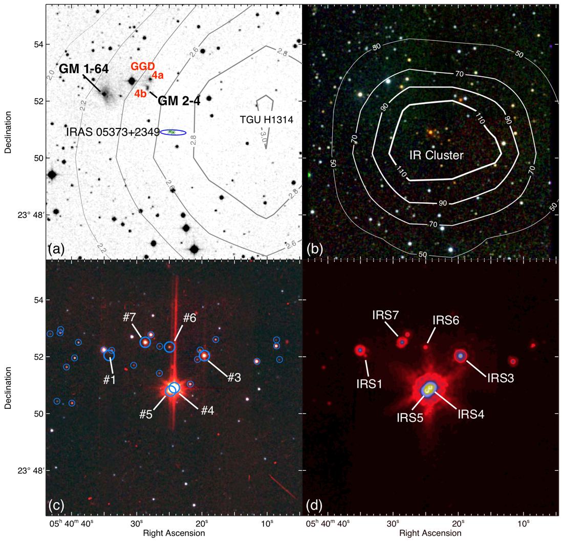
Figure 1: General field including GM 1-64 and GM 2-4 centred on IRAS 05373+2349. Panel (a) is DSS2 red image of the region overlaid with a visual extinction contours obtained from Dobashi et al. (2005) peaking at TGU H1314. The solid-line ellipse indicates the positional uncertainty of IRAS 05373+2349 and the green asterisks mark the positions of masers. Panel (b) is the 2MASS false colour composite view of the region constructed from J (blue), H (green) and K_s (red) bands. Overlaid are the IRAS 100$\mu$m contours at 50, 70, 90 and 110 MJy/sterad. Panel (c) is Spitzer IRAC colour composite image constructed from 3.6$\mu$m (blue), 4.5$\mu$m (green) and 8.0$\mu$m (red) bands. Stars marked with big and small circles are sources reported by Gutermuth et al. (2009) and classified as Class I protostars and Class II pre-main-sequence stars respectively. Panel (d) is Spitzer MIPS 24$\mu$m band view of the region where the same Class I sources are marked with the nomenclature used in our study (see Sect 3.1).

GM 2-4 was discovered on DSS1 plates (Giulbudagian & Magakian, 1977) and is classified as a Herbig-Haro-Like object (HHL 26) by Gyulbudaghian et al. (1978) and later renamed GGD 4 by Gyulbudaghian et al. (1987). Subsequent near-infrared observations (Carballo et al., 1988) were able to separate this object into two separate red nebulous objects namely GGD 4a and GGD 4b coinciding with the position of GM 2-4 (Fig. 1a). A recent continuum and narrow-band (H$\alpha$ and [SII]) optical study by Nikogossian et al. (2009) concludes that these objects (GM 2-4 and GGD 4a) are reflection nebulae and do not exhibit any Herbig-Haro characteristics. The near-infrared H₂ 1-0 S(1) line survey of Simon & Joyce (1983) did not find molecular hydrogen line emission, but this is likely due to the limited sensitivity of the infrared bolometer used in that study. The detection of an H₂O maser by Rodriguez et al. (1980) and the detection of a cold IRAS point source 05373+2349 about 1.5′south-west from the centre of GM 2-4 (cf. Fig.1a) indicated that active star-formation occurs in the region.

Casoli et al. (1986) detected high-velocity blue and red-shifted wings in the ¹²CO emission which pointed to a bi-polar outflow driven by IRAS 05373+2349. Carballo et al. (1988) obtained photometric measurements in near- to mid-infrared bands of a red object coincident with the position of the IRAS 05373+2349 using an infrared bolometer. The same red object was resolved into an infrared stellar cluster by Hodapp (1994) (cf. Fig.1b). This infrared cluster is also associated with 450$\mu$m continuum emission (Jenness et al., 1995) and with an ammonia core (Molinari et al., 1996). More recently, 3.4cm and 3.6cm continuum emission and HCO⁺ (1-0), H¹³CO⁺ (1-0) and H¹³CN (1-0) line emission were detected towards the cluster (Molinari et al., 2002). A fit to the spectral energy distribution (SED) of IRAS 05373+2349 from 8 - 1200 $\mu$m by Molinari et al. (2008) was interpreted in terms of a zero-age main-sequence B5 star of 26 M_☉ for the entire cluster of stars. The study by Gutermuth et al. (2009) using Spitzer addressed the evolutionary stages of individual members in the IR cluster, and found that its members were a mixture of Class I protostars and Class II pre-main-sequence stars with optically thick disks (cf. Fig.1c). Varricatt et al. (2010) reported some very faint near-infrared H₂ 1-0 S(1) line knots around the position of IRAS 05373+2349.

These studies demonstrate that the area around GM 2-4 is an active and on-going star formation region. We have thus decided to combine previously published data on the region with our wide-field near-infrared survey of the region in the outflow tracing H₂ 1-0 S(1) line in order to reveal the extent of outflow activity, identify their driving sources and examine the star formation processes of the studied field. In Section 2 we present the observations and the data analysis. In Section 3 we present the results from our observations, discuss the possible outflows and present SED modelling on suspected driving sources. Finally, in Section 4 we summarise our findings and present some future prospectives on the project.

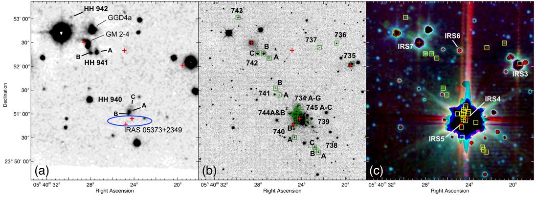
Figure 2: Close-up view of GM 2-4 and IRAS 05373+2349 including the region where new molecular hydrogen emission line objects (MHOs) are found. Class I sources reported by Gutermuth et al. (2009) are marked with a crosses on all panels. Panel (a) is optical [SII] image where Herbig-Haro objects discovered by (Nikogossian et al., 2009) are marked along with the GM 2-4, GGD 4a and IRAS 05373+2349 error ellipse. Panel (b) is near-infrared H₂ 1-0 S(1) line+continuum image where the MHOs are marked with squares. Panel (c) shows Spitzer IRAC colour-composite image constructed from 3.6$\mu$m (blue), 4.5$\mu$m (green) and 8.0$\mu$m (red) bands with positions of newly detected MHOs marked with squares for a comparison. For this particular case the brightest (mostly saturated) stars in the field were truncated in order to stretch the colour scheme and reveal relatively fainter objects.

2 Observations and Data Analysis

The following discussion makes frequent use of the optical observations by Nikogossian et al. (2009) - see that paper for a comprehensive discussion of the optical dataset.

2.1 Near-infrared Data

Observations in the near-Infrared were carried out during the night of October 11, 2004 using the Omega 2000 prime focus camera (Baumeister et al., 2003) at the Calar Alto 3.5m telescope. Omega 2000 is equipped with a 2048 $\times$ 2048 pixel HAWAII-2 array detector. It provides a pixel scale of 0.45 arcsec/pixel and a total field of view of 15.4 $\times$ 15.4 arcmin² on the sky. Images were obtained in the H₂ 1-0 S(1) line using a 1% narrow band filter centred at $\lambda$ = 2.122$\mu$m, and in a 1% narrow band continuum filter centred at $\lambda$ = 2.143$\mu$m. The total exposure time was 1500s per filter with the average seeing of $\sim$ 1.0″. The data reduction proceeded through standard routines using CCDPACK and KAPPA data reduction packages developed under the Starlink Project: i.e. the images were dark subtracted, flat fielded, sky subtracted and then combined together to form a mosaic picture of the complete field. In the next step images in $\lambda$ = 2.122$\mu$m and 2.143$\mu$m wavelengths were astrometrically calibrated and subtracted in order to reveal the pure H₂ 1-0 S(1) line emission objects in the field.

2.2 Mid-infrared Data

We acquired IRAC (Fazio et al., 2004) and MIPS (Rieke et al., 2004) data from the Spitzer Science Archive covering the area around GM 2-4. The basic flux calibrated images of the Spitzer Science Center (SSC) pipeline were used. Cosmetic corrections, astrometric refinement and the final mosaics were constructed using the MOPEX software (Makovoz & Khan, 2005). Photometric measurements were done using the aperture photometry package PHOTOM in GAIA. Instrumental values (counts/sec) where calibrated using the guidelines presented in SSC home page (i.e. appropriate aperture and pixel-scale correction) and zero-point fluxes by Reach et al. (2005) based on Vega-standard magnitudes for 1 DN/s. Our results are in excellent agreement with the values presented in Gutermuth et al. (2009) differing only by a few percent.

3 Results and Discussion

Figure 3: Area containing the MHO 735, 736 and 737. Positions of IRS objects are marked with the crosses on all panels. Dotted arrow on both panels show the possible outflow direction. Panel (a) shows the H₂ 1-0 S(1) emission. Panel (b) is a colour composite image constructed from 3.6$\mu$m (blue), 4.5$\mu$m (green) and 8.0$\mu$m (red) Spitzer IRAC bands where the position of MHO 735 is marked with a filled circle for an easy comparison and a dotted bow-shock outlines the MHO 737.

3.1 Definitions and Nomenclature

Here we give a brief reasoning on the used nomenclature for the protostellar objects referred in the following sections. We follow the Gutermuth et al. (2009) source numbering with a slight difference aiming at clarifying the overall situation in the immediate vicinity of the GM 2-4 and IRAS 05373+2349 objects. Gutermuth et al. (2009) call these objects the GGD 4 cluster of sources, but this nomenclature in our view is misleading in two ways. Firstly the actual position of the GGD 4 object reported originally by Gyulbudaghian et al. (1978) is about 1.5 arc-minutes to the north-east of the near-infrared cluster discovered by Hodapp (1994) (Fig. 1(b)). Secondly the GGD 4 object, which were later renamed GGD 4a and GGD 4b (GM 2-4) by Carballo et al. (1988), are a pair of reflection nebulae. These reflection nebulae are not associated with HH objects; nor are they obviously connected with the maser sources reported by Rodriguez et al. (1980). We believe that the cluster should be called the IRAS 05373+2349 cluster and the numbering of the infrared sources reported by Gutermuth et al. (2009) should be preserved. Therefore in the interest of brevity, and because of the absence of any other clusters in the region we will use the IR cluster and the IRS# (Infra-Red-Source) nomenclature throughout this work.

3.2 New Molecular Hydrogen emission line Objects (MHOs)

Figure 2 presents a part of our region where we detected numerous H₂ 1-0 S(1) line emission objects. In order to identify pure H₂ 1-0 S(1) line emission objects we subtracted the 2.143$\mu$m narrow-band continuum image from the 2.121$\mu$m line image. For the comparison we include optical [SII] line data (Nikogossian et al., 2009) along with the colour-composite figure constructed from Spitzer IRAC bands. We detected number of new Molecular Hydrogen emission-line Objects (Davis et al., 2010) (MHOs hereafter). Table 1 provides the coordinates, flux in units of 10^-18 W m^-2 arcsec^-2 and some additional notes related to the newly discovered MHOs. In the following subsections we briefly describe each outflow.

3.2.1 MHO 735, 736 and 737

About 2 arc-minutes west from GM 2-4 (cf. Fig. 2a,b) three emission line objects MHO 735, 736 and 737 were detected. The detailed view of the area in near-infrared H₂ 1-0 S(1) emission and the composite constructed from the Spitzer IRAC bands including these objects are presented on Fig. 3a and b.

MHO 735 is situated very close to the continuum source IRS3 which appears prominently at mid-infrared wavelengths and is most likely the driving source of MHO 735 based on the positional closeness ($\sim$ 0.018pc on 1.17kpc). We were unable to identify MHO 735 in the 3.6$\mu$m, 4.5$\mu$m and 8.0$\mu$m Spitzer IRAC bands, due to the large point spread function of IRS3 (cf. Fig.3b). In contrast MHO 736 and 737 are detected at 4.5$\mu$m as expected if the emission originates from shock excited H₂ lines (Smith & Rosen, 2005; Ybarra & Lada, 2009). A confirmation of the shocked nature in 4.5$\mu$m would require a spectroscopic follow-up.

A close examination of the colour-composite IRAC view (Fig.3b) reveals the bow-shock shape of the MHO 737 which suggests the IRS6 as a possible driving source of a flow with a length of at least 0.195pc (Tab. 2). The direction of the flow (if confirmed) would also be suitable for inclusion of MHO 736 as a forward shock making it over 0.325pc long.

Table 1: List of MHOs detected in H₂ 1-0 S(1) with cross-identifications with HH objects from Nikogossian et al. (2009) and the knots identified by Varricatt et al. (2010) are marked by [VDR]8-# nomenclature.

MHO	R.A.(2000)	Dec.(2000)	Flux†	Notes
734A	05:40:24.37	+23:51:10.6	25.5	HH 940C
734B	05:40:24.40	+23:51:07.9	23.9
734C	05:40:24.57	+23:51:05.6	12.6	within [VDR]8-3
734D	05:40:24.53	+23:51:03.3	27.8	HH 940A, [VDR]8-4
734E	05:40:24.60	+23:50:59.7	43.6	HH 940B, [VDR]8-2
734F	05:40:24.62	+23:50:56.1	7.7
734G	05:40:24.59	+23:50:53.4	11.5
735	05:40:19.43	+23:52:04.4	13.9
736	05:40:20.86	+23:52:30.1	11.8
737	05:40:22.47	+23:52:24.2	4.1
738A	05:40:22.47	+23:50:12.5	8.8
738B	05:40:22.70	+23:50:15.2	4.7
738C	05:40:22.84	+23:50:18.8	9.6
739	05:40:23.44	+23:50:49.9	18.9	[VDR]8-6
740A	05:40:24.68	+23:50:30.9	7.4
740B	05:40:24.75	+23:50:43.9	5.3
741A	05:40:26.12	+23:51:24.4	3.4
741B	05:40:26.45	+23:51:32.9	1.8
742A	05:40:27.06	+23:52:10.8	10.8
742B	05:40:27.55	+23:52:16.2	32.4	HH 941A
742C	05:40:28.11	+23:52:16.2	50.4	HH 941B
743	05:40:29.94	+23:53:02.1	10.5	HH 942
744A	05:40:25.12	+23:51:00.6	32.2	[VDR]8-2
744B	05:40:24.76	+23:51:00.6	12.3	[VDR]8-3
745A	05:40:24.10	+23:51:03.4	4.9
745B	05:40:24.14	+23:51:00.6	13.2	[VDR]8-5
745C	05:40:24.39	+23:50:52.1	23.2	[VDR]8-1

^† Flux in 10^-18 W m^-2 units and the background 1$\sigma$ noise estimate is $1.15\times 10^{-19}$ W m^-2 calculated in 6″ circular aperture

3.2.2 MHO 734, 739, 740, 744 and 745

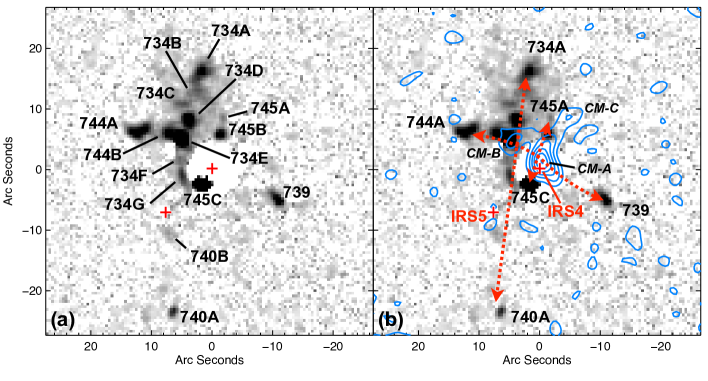
Figure 4: Close-up view in H₂ 1-0 S(1) emission of the area surrounding the IRAS 05373+2349 and the near-infrared cluster where numerous MHOs where identified. Positions of IRS4 and 5 are marked with crosses on all panels. Panel (a) reveals details of MHO 734, 739, 740, 744 and 745. Panel (b) shows the suggested outflow structure with dotted arrows. Overlaid contours are from the 3.6cm emission starting from 3$\sigma$ and climbing with a 3$\sigma$ step-size and are from the data published by Molinari et al. (2002). Positions of 3.6cm peaks are marked with CM-A, -B and -C.

A detailed view of the region around IRAS 05373+2349 (IRS4 and 5) shows a complex structure of knots and bows in the immediate vicinity of IRS4 (cf. Fig. 4a). This region has been studied by Varricatt et al. (2010) who also detected several faint H₂ 1-0 S(1) line features (object 8 in their paper) which coincide with some of the individual knots detected in our study (cf. Tab. 1 for cross-identification). In our deeper images we were able to detect more features and therefore suggest several possible outflows, which are marked on Fig. 4b and listed in Table 2.

An elongated object MHO 739 located about 10″ south-west from IRS4 was also detected by Varricatt et al. (2010) who label this feature as 8-6. This object could be connected with the MHO 744B compact knot (8-3) and MHO 744A bow-shock (8-2) to form a 0.144pc long bipolar outflow (739-744 outflow) possibly driven by IRS4/CM-A (Fig. 4b). Next bipolar flow (745flow $\sim$ 0.068pc), perpendicular to the 739-744 outflow, connecting MHO 745A and B on one side and MHO 745C on the other side is most likely driven from the very same IRS4/CM-A source (Molinari et al., 2002).

The chain of bow-shocks, compact knots and elongated features denoted as MHO 734A to G (cf. Fig. 4a) connect with the MHO 740B and 740A knots forming the third bipolar outflow (734-740 $\sim$ 0.226pc; Tab. 2) in this active region (Fig. 4b). Determination of the true driving source of this bipolar outflow is unrealistic due to the limiting dataset, but one could suggest some candidates based on a simple geometrical placement of the probable candidates. In this respect CM-B (Molinari et al., 2002) is the most probable driving source for this outflow but one could also consider IRS4/CM-A source because of its apparent closeness and prominence. Lastly the overall outflow direction described by 734-740 (Tab 2) coincides with the ¹²CO outflow reported previously by Casoli et al. (1986).

3.2.3 MHO 738 and 741

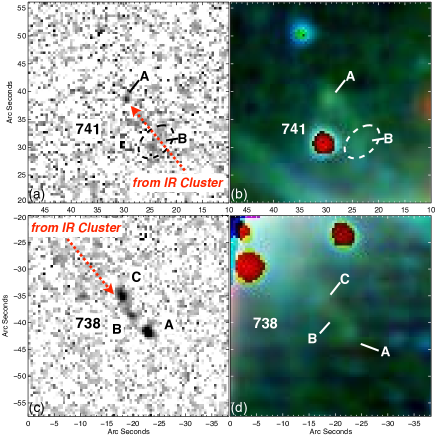
Figure 5: Scaled-up views of MHO 738 and 741 where the offsets are calculated from IRS4. Dotted-line arrows show the direction of the suggested bipolar outflow. Panel (a) shows the area including MHO 741 in H₂ 1-0 S(1) emission and the panel (b) is the same area in Spitzer IRAC composite view constructed from 3.6$\mu$m (blue), 4.5$\mu$m (green) and 8.0$\mu$m (red) bands. Panel (c) and panel (d) show the same wavelengths as in panels (a) and (b) but for the area including the MHO 738A, B and C.

Figure 5 gives the details of MHO 738 and 741 in H₂ 1-0 S(1) emission and in Spitzer IRAC composite view where the offsets are calculated from IRS4 (cf. Fig. 2).

About 40″ south-west from the IRS4 several bow-shaped features labelled MHO 738A to C are located (Fig. 5c and d). The morphology and their placement suggests that one of the sources in the IR cluster drives an outflow creating the MHO 738 A-C bow shocks. To the north-east of the IR cluster, again at a distance of about 40″  the two faint knots MHO 741A and 741B are located (Fig. 5a and b).

MHO 738 and 741 quite likely are part of yet another bipolar outflow ($\sim$ 0.498pc; Tab. 2) driven from the sources in the IR cluster. As a candidate driving source for the 738-741 outflow both IRS4/CM-A and CM-B can be considered.

3.2.4 MHO 742 and 743

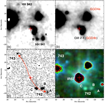
Figure 6: Region around IRS7 including MHO 742 and 743. Panel (a) is optical [SII] view where HH 941 and 942 are marked. Panel (b) is optical I-band continuum view where the reflection nebulae GM 2-4 (GGD 4b) and GGD 4a are indicated. Panel (c) is the near-infrared H₂ 1-0 S(1) line image where MHO 742 and 743 are indicated. Dotted arrow shows the suggested bipolar outflow. Panel (d) is Spitzer IRAC composite view constructed from 3.6$\mu$m (blue), 4.5$\mu$m (green) and 8.0$\mu$m (red) bands where along with MHO 742 and 743 IRS7 is also indicated.

The area around GM 2-4 has been studied recently by Nikogossian et al. (2009) who found two Herbig-Haro objects, HH 941 and HH 942. Our follow-up on the same region reveal near- to mid-infrared counterparts of these HH objects. Fig. 6 gives the optical [SII] and I-band, near-infrared H₂ 1-0 S(1) and Spitzer IRAC views of the region around the optically undetectable IRS7 which illuminates the GM 2-4 (GGD 4b) nebula. For completeness we note that GGD 4a is also illuminated by a near- to mid-infrared source which was classified as a Class II pre-main-sequence star by Gutermuth et al. (2009) (cf. Fig 1).

About 20″ south-west of IRS7 (Fig. 6c) the MHO 742 object composed of several prominent knots (A, B and C) was identified coinciding with the optical HH 941A and B (cf. Tab. 1). While knots MHO 742B and C are less defined the MHO 742A knot clearly resembles a bow-shock like structure pointing back to IRS7. Similarly about 30″ north-east of IRS7 (Fig. 6c) lays MHO 743 which has a clear bow-like morphology pointing back to the IRS7 as well. This makes 742-743 a 0.372pc long bipolar outflow (Tab 2) emanating from IRS7.

In addition all features detected in near-infrared H₂ 1-0 S(1) line are also clearly detectable in green on the Spitzer IRAC composite view (Fig. 6d) which suggests that the radiation must be coming from the shock excited H₂ lines found in IRAC 4.5$\mu$m band.

Table 2: Outflows and their driving sources for the discussed region.

MHO outflow	Source	Size (pc)†	Flux⋆	Notes
735flow	IRS3	0.018	13.9	monopolar
736flow	IRS6	0.325	15.9	monopolar
738-741	IRS4/CM-A	0.498	28.3	bipolar
739-744	IRS4/CM-A	0.144	63.1	bipolar
745flow	IRS4/CM-A	0.068	41.3	bipolar
734-740	CM-B	0.226	165.3	bipolar
742-743	IRS7	0.372	104.1	bipolar

^† Assuming 1.17kpc distance
^⋆ Combined flux in 10^-18 W m^-2 units

3.3 SED modelling of IRS Objects

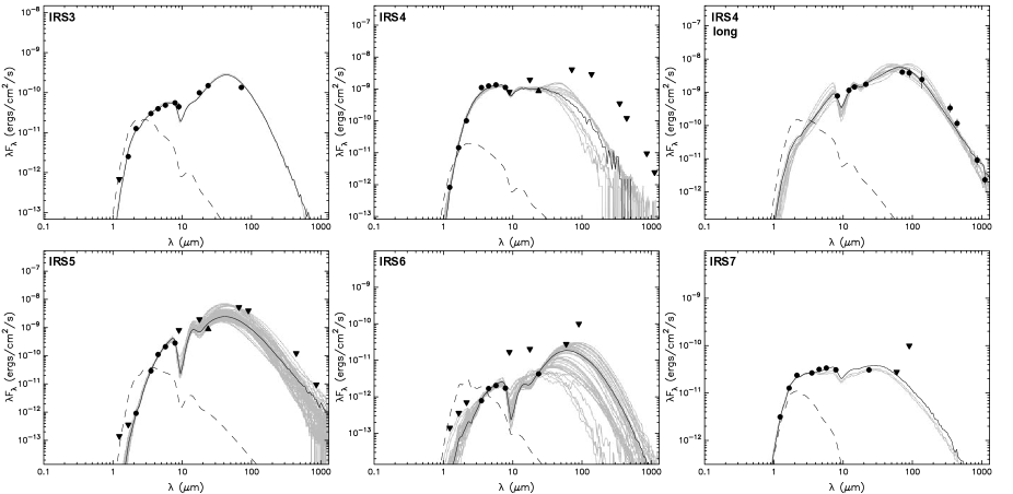
Figure 7: Spectral energy distribution (SED) of IRS3 to IRS7. Filled circles are the data points and the triangles are lower and upper limits where errors are generally smaller than the data points. The solid black line indicates the best-fitting model, and the grey lines show all models that also fit the data satisfying the $\chi^{2}$ - ${\chi}^{2}_{best}$ $<$ 3 per data point criteria. The dashed line shows the SED of the assumed stellar photosphere in the best-fitting model.

In order to better characterise the IRS objects we have explored the archive of 2D axisymmetric radiative transfer models of protostars (Robitaille et al., 2006) calculated for a large range of stellar parameters (masses, accretion rates, disk masses and disk orientations), evolutionary stages (from the early envelope infall to the late disk-only) and each calculated for 10 different viewing angles developed by Robitaille et al. (2007). The archive also provides an SED fitting interface which can be used to select best fit models to a given observed SED within the specified $\chi^{2}$. We have used this interface to input all the available magnitude/flux values for the IRS objects from various archives and databases (presented in Table 4). Those values were imputed assuming a conservative error of at least 10% in order to avoid over-interpretation of the SEDs (Robitaille et al., 2007), although the true errors are smaller in the near to mid-infrared range. The observed SED can also be scaled to match the models in the grid by using a range of values in extinction (A_V) and distance. For the distance we took range from 1 to 1.7 kpc but for IRS4 and 5 we narrowed down the range to 1-1.3 kpc, since the distance to the IR cluster (1.17 kpc) is known with higher certainty. For the A_V we used values from Gutermuth et al. (2009) with $\pm$ 10% range.

Table 3: Model best fit results (in bold face text) satisfying the $\chi^{2}$ - ${\chi}^{2}_{best}$ $<$ 3 per data point criteria for IRS objects using online SED fitting interface by Robitaille et al. (2007). Provided errors are calculated as difference between lowest and highest parameter values of SED models compared to the best fit satisfying the same criteria. See Section 3.3 for explanation and discussions.

Parameter	IRS3	IRS4	IRS4-long	IRS5	IRS6	IRS7
$M_{*}$ (M☉)	1.88$\pm^{0.00}_{0.00}$	9.90$\pm^{2.10}_{4.64}$	4.49$\pm^{1.97}_{2.57}$	3.66$\pm^{4.78}_{3.16}$	0.29$\pm^{3.43}_{0.19}$	2.24$\pm^{0.00}_{0.00}$
Age $\times 10^{4}$ (yr)	4.83$\pm^{0.00}_{0.00}$	138$\pm^{250}_{29}$	0.58$\pm^{1.98}_{0.47}$	0.22$\pm^{70.4}_{0.10}$	0.68$\pm^{982}_{0.58}$	54.6$\pm^{0.0}_{0.0}$
$R_{*}$ (R☉)	10.6$\pm^{0.0}_{0.0}$	3.97$\pm^{0.43}_{1.22}$	31.1$\pm^{9.2}_{16.3}$	26.7$\pm^{35.0}_{23.6}$	4.76$\pm^{2.54}_{3.01}$	4.93$\pm^{0.0}_{0.0}$
$T_{*}\times 10^{3}$ (K)	4.3$\pm^{0.0}_{0.0}$	25.5$\pm^{2.8}_{8.5}$	4.23$\pm^{0.22}_{0.12}$	4.21$\pm^{15.09}_{0.52}$	3.35$\pm^{9.85}_{0.81}$	4.96$\pm^{0.0}_{0.0}$
$M_{disk}\times 10^{-2}$ (M☉)	3.06$\pm^{0.00}_{0.00}$	7.55$\pm^{10.85}_{7.46}$	40.1$\pm^{13.2}_{39.7}$	20.40$\pm^{19.10}_{20.39}$	0.51$\pm^{2.63}_{0.51}$	10.6$\pm^{0.0}_{0.0}$
$\dot{M}_{disk}\times 10^{-6}$ (M☉/yr)	0.024$\pm^{0.00}_{0.00}$	0.067$\pm^{6.333}_{0.061}$	3.18$\pm^{107.82}_{3.04}$	2.88$\pm^{94.42}_{2.87}$	0.081$\pm^{97.91}_{0.081}$	1.21$\pm^{0.0}_{0.0}$
$R_{min}$ Disk (AU)	2.26$\pm^{0.00}_{0.00}$	7.87$\pm^{15.73}_{3.51}$	1.13$\pm^{11.17}_{0.24}$	5.89$\pm^{14.71}_{5.23}$	0.67$\pm^{2.32}_{0.62}$	0.33$\pm^{0.0}_{0.0}$
$R_{max}$ Disk (AU)	34.8$\pm^{0.0}_{0.0}$	285$\pm^{712}_{208}$	7.68$\pm^{77.92}_{5.03}$	11.9$\pm^{553.1}_{10.39}$	48.5$\pm^{2951.5}_{46.75}$	83.0$\pm^{0.0}_{0.0}$
$M_{env.}\times 10^{-2}$ (M☉)	6.57$\pm^{0.00}_{0.00}$	0.0000285$\pm^{8.909972}_{0.000027}$	572$\pm^{13728}_{317}$	100$\pm^{2580}_{93}$	35.8$\pm^{41.5}_{35.8}$	0.01$\pm^{0.00}_{0.00}$
$\dot{M}_{env.}\times 10^{-6}$ (M☉/yr)	8.19$\pm^{0.00}_{0.00}$	0.0$\pm^{0.004}_{0.000}$	464$\pm^{1296}_{389}$	31.9$\pm^{101.1}_{30.9}$	7.5$\pm^{24.9}_{7.5}$	0.09$\pm^{0.058}_{0.000}$
$R_{max}$ Env. $\times 10^{3}$ (AU)	3.22$\pm^{0.00}_{0.00}$	0.0$\pm^{20.2}_{0.0}$	5.04$\pm^{69.56}_{0.37}$	8.7$\pm^{69.7}_{6.1}$	5.08$\pm^{2.53}_{5.08}$	1.13$\pm^{0.0}_{0.0}$
$L_{tot}$ (L☉)	34.5$\pm^{0.0}_{0.0}$	6030$\pm^{5570}_{5450}$	290$\pm^{196}_{102}$	212$\pm^{958}_{102}$	2.68$\pm^{127.32}_{2.02}$	25.2$\pm^{0.0}_{0.0}$
Incl. Angle (deg.)	56.6$\pm^{6.7}_{0.0}$	81.4$\pm^{5.7}_{40.0}$	18.2$\pm^{0.0}_{0.0}$	31.8$\pm^{49.6}_{13.6}$	49.5$\pm^{37.6}_{31.3}$	31.8$\pm^{24.8}_{0.0}$
Fitted $A_{V}$ (mag.)	22.00$\pm^{0.00}_{1.96}$	22.68$\pm^{3.32}_{0.68}$	22.00$\pm^{1.56}_{0.00}$	38.76$\pm^{11.24}_{11.69}$	16.3$\pm^{3.7}_{2.3}$	14.91$\pm^{0.00}_{0.40}$
Fitted Distance (kpc)	1.15$\pm^{0.00}_{0.05}$	1.12$\pm^{0.17}_{0.12}$	1.23$\pm^{0.06}_{0.23}$	1.17$\pm^{0.11}_{0.17}$	1.55$\pm^{0.15}_{0.84}$	1.17$\pm^{0.05}_{0.00}$
N (models)	2	19	24	78	96	4

Figure 7 shows the SED fits for the IRS objects where the solid black line in each case represents the best fit model and the grey lines show the next best fits which satisfy the criteria of $\chi^{2}$ - ${\chi}^{2}_{best}$ $<$ 3 per data point (Robitaille et al., 2007). In the case of IRS4 we present a second set of models which better fit the long wavelengths part of the SED (IRS4 long). Results from the fits are then listed in Table 3 where first column lists the names of fitted parameters and in all subsequent columns the parameters of SED fits are given for each IRS object.

Before discussing each object and determining how accurate the derived physical parameters are from the given SED fit, we would like to address some of the general discrepancies that one could expect from the procedure itself. We emphasise that the SED fitter is not a tool to accurately derive the physical parameters but it provides a way to determine how well constrained each of the different parameters are (Robitaille et al., 2007). Those parameters strongly depend on the wavelength coverage for each object and are better constrained by the multi-waveband data points from the near-infrared to radio (see Table 4 for our coverage).

In cases when the observed data-points were enough to fit a relatively accurate SED there have been some cases (CoKu Tau/1 and GG Tau for example) when the derived parameters where quite unrealistic when compared with the observed data and the independent theoretic analysis (see Robitaille et al., 2007, for the details). The SED fitter uses pre-compiled grid of model SED (Robitaille et al., 2006) to derive the physical parameters and as numerous as they are it would be naive to suggest that we have a complete coverage of all the possible nuances that influence or drive the star formation process. We would like to note that it is not the scope of this work to give exhaustive explanation to all those discrepancies but rather to use these SED fits as first approximation or as a work in progress.

3.3.1 IRS3

IRS3 was previously reported to be a Class I protostar by Gutermuth et al. (2009) using near to mid-infrared colour-colour analysis. Our SED modelling gives a good fit (Fig. 7) which is largely due to the numerous multi-waveband data points (1.2 to 70 $\mu$m) present for the object. The degeneracy or number of models satisfying the best-fit criteria is just 2 with slight difference in disk inclination angle, fitted distance and the fitted A_V (Tab. 3). The fitted distance ($\sim$1.15kpc) is in good agreement with the value inferred from the observations of the IR cluster (Molinari et al., 1996). The same can be said about the fitted A_V ($\sim$20–22) which is also in a good agreement with the value derived by Gutermuth et al. (2009). The error in fitted inclination angle is not unexpected since this is one of the least well determined parameters in the SED fitting process but it is directly connected with the discrepancy in distance and A_V determination which is the result of an input $\pm$10% assumed range.

The rest of the fitted parameters do not show any degree of degeneracy. However, due to the fact that our data does not extend beyond the Spitzer MIPS 70$\mu$m we suspect that some of the parameters are not well constrained. In particular the absence of any (sub)mm data points makes the precise estimates of the disk mass ($M_{disk}$) questionable and introduces a degeneracy between the central source temperature ($T_{*}$) and the disk accretion rate ($\dot{M}_{disk}$). On the other hand we can stipulate that SED fit can not be interpreted by disk-only source but there is a significant rise after $\sim$20$\mu$m which can only be interpreted by the presence of an envelope and its higher rate of accretion ($\dot{M}_{env.}$) (Robitaille et al., 2006). This last point strongly supports the protostellar nature of the IRS3 object confirming the findings by Gutermuth et al. (2009). The classification of this source and the positional placement in regards to MHO 735 leaves no doubt that IRS3 is the driving source of a short (0.028pc) outflow.

3.3.2 IRS4 and IRS4 long

IRS4 is one of the prominent members of the IR Cluster. It has been observed at multiple wavelengths between 1.2 to 1300$\mu$m (as can be seen from the fitted SED (Fig. 7). The prominence of this object enabled its early discovery as a red source called CPM 19 which was then resolved into IR Cluster (Campbell et al., 1989; Carballo et al., 1988; Hodapp, 1994), as noted in Section 1. Recently Nikogossian et al. (2009) observed the same object in optical I and R bands and reported about the variability comparing DSS1, DSS2 and current data. In addition to these facts IRS4 was classified as a Class I protostar by Gutermuth et al. (2009) based on near to mid-infrared colour-colour analysis.

The observational facts would seem to suggest that IRS4 is quite an energetic source and it would be misleading to place it into one or other classification group. Long-wave observations suggest a possibility of high-mass source (Molinari et al., 2008) which would make low-mass classification of YSOs incompatible or inaccurate. It is worth mentioning that all of the previous infrared to radio observations were done using larger apertures which would invalidate any kind of comparison with the current near to mid-infrared data due to the IR Cluster source contamination. With these facts in hand we performed two separate SED fittings of IRS4 object; in one SED fit we used only near to mid-infrared data obtained with a small aperture ($\sim$5000AU) and the other we used large-aperture ($\sim$22000AU) data to incorporate the flux values (such as MSX6, c.f. Tab. 4) from lower resolution mid-infrared to radio wavelengths (IRS4 long). Taking into consideration all the possible discrepancies in the data points it would be almost impossible to correctly derive any physical parameters. However, as a first approximation we tried to give some interpretations noting the highly speculative nature of them.

When we fit an SED to the near to mid-infrared data points (Fig. 7) we get edge-on system containing zero age main sequence star or ZAMS of about 10M$\sun$ with almost no envelope and relatively small accreting disk. The fitted temperature would seem to indicate a spectral type of late O or early B with total luminosity of 6000 L$\sun$ which would explain its observability in all the wavelengths. In contrast, if we fit the data-points represented by larger aperture observations (Fig. 7) we get about 4.5M$\sun$ Class 0/I actively accreting protostar with a large envelope which would seem to fit the role of outflow-driving source. Both of these fits have considerable level of degeneracy which is understandable due to the uncertainties in the apertured used (Tab. 3).

This kind of clear separation between sources fitted using the different apertures suggests a possibility of multiple objects in the line of sight belonging to the same IR Cluster. It would seem that the visible IRS4 is situated in front of an embedded core which probably contains Class 0/I protostar coinciding with the CM-A core (Fig. 4). This kind of superimposition would explain the abundance of outflows from the same area but it would be difficult to stipulate which outflow belongs to which source since there is a possibility of more hidden objects along the line of sight.

3.3.3 IRS5

IRS5 is one of the Class I sources identified by Gutermuth et al. (2009) which is almost invisible at near-infrared wavelengths. The picture is quite different in mid to far-infrared bands where IRS5 even outshines IRS4 (24$\mu$m on Fig. 1; Tab. 4). Our analysis of this object provides a challenge due to its apparent closeness to IRS4, preventing accurate PSF flux measurements. Similar discrepancies are also invalidating some of the flux values presented in various catalogues forcing us to use them only as upper-limits which rises the degeneracy of the SED fits (Tab. 3). Despite that, from the SED fit (Fig. 7) we can derive some reasonable characterisation for IRS5.

IRS5 is one of the deeply embedded members of this IR Cluster of stars. Our SED fit suggests a very young Class 0/I protostar possibly in the same stage as CM-A core discussed in Sect. 3.3.2. There was no 3.6cm core reported in this position (cf. Fig. 4) within 3$\sigma$ limit of the observations (Molinari et al., 2002) but there is a hint of a possible object below or around that limit which would need to be followed by separate observations. IRS5 could be the driving source of the MHO 740A and B flow but those MHOs seem to be aligned with the knots in MHO 734 and are likely being driven from the CM-B core rather than from IRS5, which is not well aligned with the axis of this MHO outflow (Fig. 4).

3.3.4 IRS6

One of the possible candidates of outflow driving sources in the presented region is IRS6. This object was identified as a Class I YSO by Gutermuth et al. (2009), based solely on its mid-IR colours (it is undetected in the near-IR). The scarceness of valid data points throughout the whole electromagnetic spectrum prevented us from producing a reliable SED fit for IRS6 as can be seen from Fig. 7 and Tab. 3. The best fit SED values seem to indicate a young Class 0/I low-mass star (0.29M$\sun$) situated relatively further (1.55kpc) than the rest of the IRS objects being discussed here. All of the fitted parameters in this case are very sensitive to the range of A_V used which is still uncertain for this particular source. In our fit we assumed range of 14 - 20 based on the fact that values of 14 to 20 were reported for IRS7 and IRS3 respectively by Gutermuth et al. (2009) and IRS6 is situated in-between.

3.3.5 IRS7

IRS7 is the star which illuminates the GM 2-4 (GGD 4b) optical reflection nebula and is the probable driving source of the MHO 742-743 outflow (Fig. 6). We have relatively well sampled data points from near to mid-infrared range of electromagnetic spectrum which enabled us to produce quite good SED fit as can be seen on Fig. 7. Following the same logic as we did in case of IRS3 (see Sect. 3.3.1) we can suggest that the best fit SED parameters (cf. Tab. 3) infer relatively evolved Class II YSO rather than Class I as suggested by Gutermuth et al. (2009). We find that IRS7 is a low-mass YSO with active accreting disk which is dominating the emission coming from this source. All the fitted SED parameters enforce our scenario of IRS7 being the driving source of the 742-743 bipolar outflow.

3.4 Star Formation in the vicinity of GM 2-4

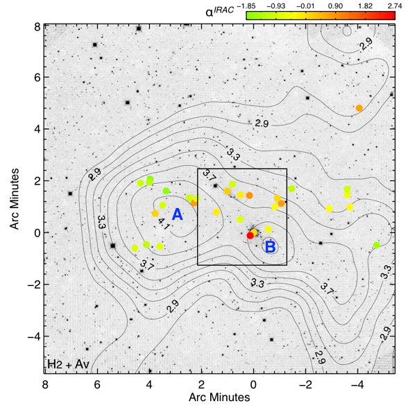
Figure 8: The wide-field view of the region in H₂ where offsets are measured from IRS4 and solid line box shows the area presented in Fig. 2(b). Overlaid contours are from A_V map constructed from 2MASS PSC and provided by Rowles & Froebrich (2009). Filled circles indicate the positions of IRAC identified Class I/II YSO sources provided by Gutermuth et al. (2009) where the colour spans according to the range of IRAC SED Slope ($\alpha^{IRAC}$).

Fig. 8 shows the wide-field area where the search for outflows was performed. However, MHO flows were only detected in a small sub-region presented in Fig. 2(b). This suggests that the immediate vicinity of the IRS3 to IRS7 is the site of relatively recent star formation activity. This scenario becomes even more favourable if we consider the disk prominence of the YSOs as defined by the parameter $\alpha^{IRAC}$ (the slope of the SED across the mid-infrared wavelengths observed with the IRAC instrument on Spitzer) and their overall distribution in East and West of the area. There are more Class II or weak-disk sources in the East than in the west.

Furthermore let us consider $\alpha^{IRAC}$ and the relative distribution of the YSOs to the two distinct A_V peaks (A and B) shown on Fig. 8. Most of the YSOs with significant circumstellar disks are associated with the A_V peaks but not strictly confined to the peaks which could generally be due to the dispersal of protostars from their original birthplace showing somewhat uniform spread in relation to the A_V peaks as it can be seen in case of peak A. This would mean that YSO population associated with peak A could have already gone through the active phase of star formation and therefore had time to disperse almost uniformly in relation to the peak A and have more evolved appearance.

The same could not be said for the YSO population associated with the peak B (Fig. 8) since in this case there is no uniform distribution rather than the protostars are situated in the North-East part of the peak suggesting that the star formation progresses from North-East to West, South-West for the entire region discussed here. This is in good agreement with the scenario of star formation around A_V peak A and non-detection of outflows in that area.

4 Summary

We have presented near-infrared H₂ 1-0 S(1) line study of the region surrounding GM 2-4 alternatively known as GGD 4 in order to reveal the outflow content of the area and to better understand the earlier suspected star formation processes in this area. In our quest to understand this region we combined multi-waveband data-sets obtained from various online archives. Our findings and analysis can be summarised as following:

• The analysis of our near-infrared H₂ 1-0 S(1) line data enabled us to identify 27 individual shocked features which combine into 5 bipolar and 2 monopolar outflows driven from the protostars in the immediate vicinity of the GM 2-4 reflection nebula. We were able to cross-correlate some of the H₂ identified objects with previously reported optical HH objects as well as with green fuzzy features in Spitzer IRAC 4.5$\mu$m wide-field band thought to have a shocked nature.

• We were able to propose the driving sources for the detected outflows based on the morphological and positional characteristics of the individual shocked features. All of the driving sources were identified as YSO based on the previously available knowledge (Gutermuth et al., 2009; Nikogossian et al., 2009) and our SED modelling. In one particular case, IRS4, our SED modelling enabled us to suggest a solution for the previously known discrepancy (Molinari et al., 1996, 2002) as two different stars one late O to early B type 10M$\sun$ ZAMS high mass star and the other as very early, possibly Class 0 protostar on the same line of sight which might be the actual driving source of the several bipolar outflows.

• Our analysis of the wide area using IRAC SED Slope in conjunction with the A_V map including the GM 2-4 suggests that star formation progresses roughly from North-East to West, South-West. This result confirms the conclusion made in our previous paper (Nikogossian et al., 2009) mainly on the base of the optical data.

There are still several facts that we wish to follow-up in order to understand the exact outflow dynamics involved in the IR cluster for which further high-resolution imaging, spectroscopy and radio-line data would be beneficiary. The importance of spectroscopic followup and monitoring of IRS4 (CPM19) would prove useful in determining the exact nature of variability in this object.

Appendix A Photometry

Table 4: Photometric value database for all IRS object converted into mJy with the appropriate errors and used apertures to model SEDs. Origin of the each data-set is indicated in the last column.

Filter	IRS3$\pm$Err. (Ap.$\arcsec$)	IRS4$\pm$Err. (Ap.$\arcsec$)	IRS5$\pm$Err. (Ap.$\arcsec$)	IRS6$\pm$Err. (Ap.$\arcsec$)	IRS7$\pm$Err. (Ap.$\arcsec$)	Data†
2MASS J	$<$0.282 (3)	0.344$\pm$0.046 (5)	$<$0.058 (4)	$\ldots$	1.294$\pm$0.059 (4)	(1)
2MASS H	1.400$\pm$0.087 (3)	8.029$\pm$0.247 (5)	$<$0.199 (4)	$\ldots$	7.065$\pm$0.230 (4)	(1)
2MASS K	9.118$\pm$0.329 (3)	73.236$\pm$2.127 (5)	0.661$\pm$0.086 (4)	$\ldots$	17.074$\pm$0.465 (4)	(1)
IRAC Ch1	35.690$\pm$0.972 (5)	1307.831$\pm$11.990 (5)	34.084$\pm$0.622 (4)	0.930$\pm$0.008 (4)	31.373$\pm$0.287 (5)	(2),(3)
IRAC Ch2	59.504$\pm$2.152 (5)	1864.438$\pm$17.093 (5)	166.935$\pm$1.530 (4)	2.527$\pm$0.023 (4)	47.703$\pm$0.437 (5)	(2),(3)
IRAC Ch3	93.046$\pm$3.365 (5)	2586.412$\pm$23.712 (5)	398.747$\pm$3.656 (4)	3.915$\pm$0.036 (4)	64.967$\pm$0.596 (5)	(2),(3)
IRAC Ch4	145.566$\pm$3.967 (5)	2931.306$\pm$26.874 (5)	743.124$\pm$6.813 (4)	4.561$\pm$0.124 (4)	81.482$\pm$0.747 (5)	(2),(3)
MSX6 A	193.8$\pm$13.6 (15)	$<$2169.7 (15)	$\ldots$	$\ldots$	$\ldots$	(4)
AKARI/IRC 9	135.82$\pm$0.223 (5)	2411.56$\pm$175.4 (8)	$\ldots$	$\ldots$	$\ldots$	(5)
IRAS 12	$\ldots$	$<$9020 (30)	$\ldots$	$\ldots$	$\ldots$	(6)
MSX6 C	$\ldots$	$<$4652.9 (15)	$\ldots$	$\ldots$	$\ldots$	(4)
MSX6 D	798.1$\pm$79.8 (15)	$<$7098.3 (15)	$\ldots$	$\ldots$	$\ldots$	(4)
AKARI/IRC 18	588.53$\pm$57.9 (6)	11499.8$\pm$53.4 (10)	$\ldots$	$\ldots$	$\ldots$	(5)
MSX6 E	$\ldots$	$<$12474 (15)	$\ldots$	$\ldots$	$\ldots$	(4)
MIPS 24	1174.08$\pm$31.99 (7)	$>$6768.59 (4)	$>$6945.42 (4)	33.55$\pm$1.21 (5)	243.05$\pm$2.23 (7)	(2),(3)
IRAS 25	$\ldots$	$<$305560 (30)	$\ldots$	$\ldots$	$\ldots$	(6)
IRAS 60	$\ldots$	$<$144830 (30)	$\ldots$	$\ldots$	$\ldots$	(6)
AKARI/FIS 65	$\ldots$	115140$\pm$7332 (30)	$\ldots$	$\ldots$	$\ldots$	(7)
MIPS 70	$<$3223 (30)	$<$96926 (30)	$\ldots$	$\ldots$	$\ldots$	(3)
AKARI/FIS 90	$\ldots$	$<$120067 (30)	$\ldots$	$\ldots$	$\ldots$	(7)
IRAS 100	$\ldots$	$<$191160 (38)	$\ldots$	$\ldots$	$\ldots$	(6)
AKARI/FIS 140	$\ldots$	132767$\pm$23968 (30)	$\ldots$	$\ldots$	$\ldots$	(7)
AKARI/FIS 160	$\ldots$	239313$\pm$3880.5 (30)	$\ldots$	$\ldots$	$\ldots$	(7)
350$\mu$m	$\ldots$	$<$41000 (30)	$\ldots$	$\ldots$	$\ldots$	(8)
SCUBA 450$\mu$m	$\ldots$	$<$18000 (30)	$\ldots$	$\ldots$	$\ldots$	(8)
SCUBA 850$\mu$m	$\ldots$	$<$2730 (35)	$\ldots$	$\ldots$	$\ldots$	(8)
1.1mm	$\ldots$	$<$910 (30)	$\ldots$	$\ldots$	$\ldots$	(8)
1.3mm	$\ldots$	$<$700 (30)	$\ldots$	$\ldots$	$\ldots$	(8)

^† Data origin: (1) 2MASS by Skrutskie et al. (2006); (2) Gutermuth et al. (2009); (3) this publication; (4) MSX6 PSC by Egan et al. (2003); (5) AKARI/IRC by Ishihara et al. (2010); (6) IRAS PSC; (7) AKARI/FIS by Kawada et al. (2007); (8) Molinari et al. (2000).

References

- Baumeister et al. (2003) Baumeister H., Bizenberger P., Bayler-Jones C. A. L., Kovács Z., Röser H., Rohloff R., 2003, in M. Iye & A. F. M. Moorwood ed., Society of Photo-Optical Instrumentation Engineers (SPIE) Conference Series Vol. 4841 of Presented at the Society of Photo-Optical Instrumentation Engineers (SPIE) Conference, Cryogenic engineering for OMEGA2000: design and performance. pp 343–354
- Brand & Blitz (1993) Brand J., Blitz L., 1993, A&A, 275, 67
- Campbell et al. (1989) Campbell B., Persson S. E., Matthews K., 1989, AJ, 98, 643
- Carballo et al. (1988) Carballo R., Mampaso A., Eiroa C., 1988, MNRAS, 232, 497
- Casoli et al. (1986) Casoli F., Combes F., Dupraz C., Gerin M., Boulanger F., 1986, A&A, 169, 281
- Chatterjee et al. (2009) Chatterjee S., Brisken W. F., Vlemmings W. H. T., Goss W. M., Lazio T. J. W., Cordes J. M., Thorsett S. E., Fomalont E. B., Lyne A. G., Kramer M., 2009, ApJ, 698, 250
- Cohen (1980) Cohen M., 1980, AJ, 85, 29
- Davis et al. (2010) Davis C. J., Gell R., Khanzadyan T., Smith M. D., Jenness T., 2010, A&A, 511, A24+
- Dobashi et al. (2005) Dobashi K., Uehara H., Kandori R., Sakurai T., Kaiden M., Umemoto T., Sato F., 2005, PASJ, 57, 1
- Egan et al. (2003) Egan M. P., Price S. D., Kraemer K. E., Mizuno D. R., Carey S. J., Wright C. O., Engelke C. W., Cohen M., Gugliotti M. G., 2003, VizieR Online Data Catalog, 5114, 0
- Fazio et al. (2004) Fazio G. G., Hora J. L., Allen L. E., Ashby M. L. N., Barmby P., Deutsch L. K., Huang J., Kleiner S., Marengo M., Megeath S. T., and 55 coauthors 2004, ApJS, 154, 10
- Giulbudagian & Magakian (1977) Giulbudagian A. L., Magakian T. I., 1977, Akademiia Nauk Armianskoi SSR Doklady, 64, 104
- Gutermuth et al. (2009) Gutermuth R. A., Megeath S. T., Myers P. C., Allen L. E., Pipher J. L., Fazio G. G., 2009, ApJS, 184, 18
- Gyulbudaghian et al. (1978) Gyulbudaghian A. L., Glushkov Y. I., Denisyuk E. K., 1978, ApJ, 224, L137+
- Gyulbudaghian et al. (1987) Gyulbudaghian A. L., Gyul’Budagyan A. L., Rodríguez L. F., Mendoza-Torres E., 1987, Revista Mexicana de Astronomia y Astrofisica, 15, 53
- Gyulbudaghian & Maghakian (1977) Gyulbudaghian A. L., Maghakian T. Y., 1977, Soviet Astronomy Letters, 3, 58
- Hodapp (1994) Hodapp K., 1994, ApJS, 94, 615
- Ishihara et al. (2010) Ishihara D., Onaka T., Kataza H., Salama A., Alfageme C., Cassatella A., Cox N., García-Lario P., Stephenson C., Cohen M., and 23 coauthors 2010, A&A, 514, A1+
- Jenness et al. (1995) Jenness T., Scott P. F., Padman R., 1995, MNRAS, 276, 1024
- Kawada et al. (2007) Kawada M., Baba H., Barthel P. D., Clements D., Cohen M., Doi Y., Figueredo E., Fujiwara M., Goto T., Hasegawa S., and 50 coauthors 2007, PASJ, 59, 389
- Kawamura et al. (1998) Kawamura A., Onishi T., Yonekura Y., Dobashi K., Mizuno A., Ogawa H., Fukui Y., 1998, ApJS, 117, 387
- Makovoz & Khan (2005) Makovoz D., Khan I., 2005, in P. Shopbell, M. Britton, & R. Ebert ed., Astronomical Data Analysis Software and Systems XIV Vol. 347 of Astronomical Society of the Pacific Conference Series, Mosaicking with MOPEX. pp 81–+
- Molinari et al. (1996) Molinari S., Brand J., Cesaroni R., Palla F., 1996, A&A, 308, 573
- Molinari et al. (2000) Molinari S., Brand J., Cesaroni R., Palla F., 2000, A&A, 355, 617
- Molinari et al. (2008) Molinari S., Pezzuto S., Cesaroni R., Brand J., Faustini F., Testi L., 2008, A&A, 481, 345
- Molinari et al. (2002) Molinari S., Testi L., Rodríguez L. F., Zhang Q., 2002, ApJ, 570, 758
- Movsessian et al. (2008) Movsessian T. A., Magakian T. Y., Nikogossian E. H., Bally J., 2008, Astrophysics, 51, 181
- Nikogossian et al. (2009) Nikogossian E. H., Magakian T. Y., Movsessian T. A., Khanzadyan T., 2009, Astrophysics, 52, 501
- Reach et al. (2005) Reach W. T., Megeath S. T., Cohen M., Hora J., Carey S., Surace J., Willner S. P., Barmby P., Wilson G., Glaccum W., Lowrance P., Marengo M., Fazio G. G., 2005, PASP, 117, 978
- Rieke et al. (2004) Rieke G. H., Young E. T., Engelbracht C. W., Kelly D. M., Low F. J., Haller E. E., Beeman J. W., Gordon K. D., Stansberry J. A., Misselt K. A., and 33 coauthors 2004, ApJS, 154, 25
- Robitaille et al. (2007) Robitaille T. P., Whitney B. A., Indebetouw R., Wood K., 2007, ApJS, 169, 328
- Robitaille et al. (2006) Robitaille T. P., Whitney B. A., Indebetouw R., Wood K., Denzmore P., 2006, ApJS, 167, 256
- Rodriguez et al. (1980) Rodriguez L. F., Moran J. M., Ho P. T. P., Gottlieb E. W., 1980, ApJ, 235, 845
- Rowles & Froebrich (2009) Rowles J., Froebrich D., 2009, MNRAS, 395, 1640
- Simon & Joyce (1983) Simon T., Joyce R. R., 1983, ApJ, 265, 864
- Skrutskie et al. (2006) Skrutskie M. F., Cutri R. M., Stiening R., Weinberg M. D., Schneider S., Carpenter J. M., Beichman C., Capps R., Chester T., Elias J., 21 coauthors 2006, AJ, 131, 1163
- Smith & Rosen (2005) Smith M. D., Rosen A., 2005, MNRAS, 357, 1370
- Varricatt et al. (2010) Varricatt W. P., Davis C. J., Ramsay S., Todd S. P., 2010, MNRAS, 404, 661
- Ybarra & Lada (2009) Ybarra J. E., Lada E. A., 2009, ApJ, 695, L120