Simple Adaption of Measurements for Qu$d$it Estimation

Abstract

We present a strategy for estimation of $d$-level quantum states and for the simple adaption of corresponding measurements. The adaption method is inspired by mutually unbiased measurements, but it is also applicable in cases for which no complete set of mutually unbiased bases is known. We present results of Monte Carlo simulations, that demonstrate the fidelity gain of the adaptive strategy compared to a non-adaptive estimation.

1 Introduction

From the viewpoint of fundamental quantum mechanics as well as from the viewpoint of practical applications in quantum information science, determining the state of a quantum system Paris and Řeháček (2004); Raymer (1997) is an important problem, very different from the measuring process in classical physics. Perfect reconstruction of a completely unknown quantum state requires an infinite amount of measurements for various non-commuting observables. One thus also needs an infinite number of identical quantum systems. However, due to the no-cloning theorem Dieks (1982); Wootters and Zurek (1982) they cannot be copies of a single system. As a consequence, initial copies, or more exactly, identically prepared systems, are a valuable resource. From this limited resource only a limited amount of information can be extracted.

This contribution aims at an optimised utilisation of this resource for the estimation of a pure $d$-level quantum state by single measurements. The benchmark for the quality of such a procedure is the optimal average fidelity of a joint measurement Massar and Popescu (1995); Derka et al. (1998); Bruß and Macchiavello (1999) on all systems of the finite sample. However, the needed physical principles for such collective measurements are easily realised. Hence we will analyse how well this optimal method can be approximated by an approach using measurements on single copies and an adaptive choice of measurement parameters.

For qubits such single-copy measurements have been described for pure Hradil et al. (2000); Bagan et al. (2002, 2005) and mixed states Bagan et al. (2006). An adaptive method has been reported in Fischer et al. (2000) for qubits as well. There it was possible to come quite close to the theoretical limit given in Massar and Popescu (1995). For higher dimensional states single measurement schemes based on maximum likelihood estimation Hradil (1997); Paris and Řeháček (2004) and mutually unbiased measurements Wootters and Fields (1989) have already been used in experiments Klimov et al. (2008); Adamson and Steinberg (2010); Lima et al. (2011). However the application of adaptive methods to higher dimensions is not straightforward. The methods used for estimation and adaption cannot be easily calculated in general, and the numerical expense to simulate these methods efficiently turns out to be quite high. Therefore, alternative and simpler methods are needed. Before we explain these in detail, let us recall the basic problem.

2 Basic Concepts

A finite number of identically prepared versions of a $d$-dimensional quantum system shall be given. We have no prior information on the corresponding pure state $\left|\psi\right>$ and want to infer it from the results of single measurements. To this end, on one hand we have to reasonably estimate a state $\left|\psi^{\mathrm{est}}\right>$ from already gathered data (estimation). On the other hand we have to decide which measurement parameters to use for further measurement steps (adaption). We restrict ourselves to projective measurements, which can be realised in principle. Hence the main question is for the appropriate choice of the measurement basis $\left\{\left|b_{i}\right>\right\}$. This choice can be influenced by previously accumulated measurement data only. Therefore, in the beginning we can use an arbitrary basis, e.g. the computational basis. But after the first measurement we can adapt the next basis according to the previous results, conduct this measurement, and continue as long as there are copies left.

In the end, we have acquired a sequence of used measurement bases and the corresponding results, i. e. which vector of each basis was really found in the measurement. Based on this measurement data we perform the estimation procedure, which gives us the estimated state $\left|\psi^{\mathrm{est}}\right>$. To assess the quality of estimation, we can use the fidelity $F=\left|\left<\psi\vphantom{\psi^{\mathrm{est}}}\right|\left.\psi^{\mathrm{est}}\vphantom{\psi}\right>\right|^{2}$. In general, it will of course be different for different unknown states $\left|\psi\right>$. But more importantly, due to the probabilistic nature of quantum measurements the fidelity even differs for different measurement runs with the same state $\left|\psi\right>$. While we expect from a good estimator to work equally well for all unknown states, the dependence on the measurement results is inevitable. Therefore, to arrive at a valid criterion for characterising the adaptive procedure, we have to average over all possible results. In practise we achieve this by averaging over sufficiently many Monte Carlo simulations of such measurement runs.

3 Estimation

The key part of state estimation is transforming the measurement data into an estimate of the unknown quantum state. A useful method for qubits is maximum likelihood estimation Hradil (1997); Paris and Řeháček (2004). But due to the growing number of state parameters in higher dimensions sooner or later this becomes highly involved. This is equally well a problem for an experimenter, who has to find an estimate for an unknown state, as for a theoretician, who wants to assess numerically the quality of a measurement scheme. The latter has to cope with the additional complication that one has to average over a statistically significant number of simulated measurement runs.

Therefore we propose another much more primitive estimation method. For qubits this means calculating the average of the Bloch vectors corresponding to the measured states and using this average as representation of a (mixed) estimated state. In order to get a pure estimated state, this Bloch vector can be normalised. This can be viewed as a very rough simplification of maximum likelihood estimation, because the likelihood function for a single measurement is centred at the measured point on the Bloch sphere and the likelihood for more measurements is the product of such elementary likelihoods. Since a Bloch vector is nothing more than a representation of the density matrix, this is the same as directly calculating the average density matrix and choosing the pure state nearest to this average matrix.

This simple averaging procedure can be generalised to higher dimensions $d$. As in the qubit case a geometric representation of the state can be used. One such generalisation of the Bloch vector, that allows this averaging procedure, is the coherence vector Hioe and Eberly (1981); Mahler and Weberruß (1995). On the other hand the average density matrix $\hat{\overline{\rho}}$ can be calculated directly: We simply add all found measurement results $\left\{\left|m_{k}\right>\right\}$ incoherently and arrive at

$$\hat{\overline{\text{$\rho$}}}=\tfrac{1}{\nu}\sum_{k=1}^{\nu}\left|m_{k}\vphantom{m_{k}}\right>\left<m_{k}\vphantom{m_{k}}\right|$$ (1)

after $\nu$ measurements. However, in the subsequent search for a pure estimated state, a new complication arises, compared to the $d=2$ case, where it was sufficient to normalise the Bloch vector of $\hat{\overline{\rho}}$.

In order to find the pure state in best agreement with the measured data, we choose as estimated state $\left|\psi^{\mathrm{est}}\right>$ the one with maximal overlap with the averaged density operator $\hat{\overline{\rho}}$. For eigenvalues $e_{j}$ and eigenvectors $\left|e_{j}\right>$ of $\hat{\overline{\rho}}$ we arrive at

$$\left<\psi^{\mathrm{est}}\right|\hat{\text{$\overline{\rho}$}}\left|\psi^{\mathrm{est}}\right>=\sum_{j=0}^{d-1}e_{j}\left|c_{j}\right|^{2}.$$ (2)

with $c_{j}=\left<e_{j}\vphantom{\psi^{\mathrm{est}}}\right|\left.\psi^{\mathrm{est}}\vphantom{e_{j}}\right>$. When we arrange the eigenvalues in descending order $e_{0}\geq e_{1}\geq\ldots\geq e_{d-1}$, we find

$$\left<\psi^{\mathrm{est}}\right|\hat{\text{$\overline{\rho}$}}\left|\psi^{\mathrm{est}}\right>\leq e_{0},$$ (3)

where equality holds only if $c_{0}=1$ and all other coefficients vanish.

This means that the wanted estimate $\left|\psi^{\mathrm{est}}\right>=\left|e_{0}\right>$ is the eigenvector corresponding to the largest eigenvalue $e_{0}$ of $\hat{\overline{\rho}}$ (and the eigenvalue $e_{0}$ itself is the overlap of $\hat{\overline{\rho}}$ and $\left|\psi^{\mathrm{est}}\right>$). Thus the estimation procedure consists of two numerically simple steps: incoherent superposition of the measured states and solving the eigenvalue problem of the averaged density matrix. For a comparison of this estimation scheme to other possible estimators applied to non-adaptive measurement setups see Bschorr et al. (2006).

4 Least Bias Adaption

We have described a method for calculating estimated states from measurement data; but we still have to decide which measurement bases to use. In the qubit case it was possible to formulate an expected fidelity with respect to the used measurement parameters and to find the optimal parameters by maximising this expected fidelity Fischer et al. (2000); Happ and Freyberger (2008). Again this becomes a tedious numerical task in higher dimensions. Instead we use a method that mimics mutually unbiased bases (MUBs) Wootters and Fields (1989).

Two bases $\left\{\left|b_{i}\right>\right\}$ and $\left\{\left|b_{j}^{\prime}\right>\right\}$ are called unbiased if each pair of basis vectors from different bases has the same overlap

$$\left|\left<b_{i}\vphantom{b_{j}^{\prime}}\right|\left.b_{j}^{\prime}\vphantom{b_{i}}\right>\right|^{2}=\tfrac{1}{d}.$$ (4)

In $d$ dimensions there are up to $d+1$ bases that are mutually unbiased Durt et al. (2010). Such sets of MUBs are optimal for state estimation with fixed measurements on single copies in the sense of minimising statistical errors Wootters and Fields (1989); Lima et al. (2011). However, as soon as there are more measurements performed than are MUBs known, it is possible to find measurement strategies that improve estimation fidelity compared to repeated MUB measurements Bagan et al. (2002). Our least bias adaption method broadens the idea of mutually unbiased measurements for use with more measurements.

The ultimate goal of adaption is finding measurement parameters that maximise the information gained in this measurement. Mutually unbiased measurements ensure exactly that, because each sequence of possibly measured state vectors is “unbiased”, having overlap $\tfrac{1}{d}$ with each other. However, since the measurements are made successively, mutual unbiasedness is sufficient but not necessary for this maximised information gain. Only the actually measured basis vector has to be remembered from each measurement; the directions of the other basis vectors are irrelevant. Therefore the next measurement basis has to be “unbiased” with respect to the previous measurement results but not to the previous measurement basis vectors which were never actually found in a measurement. Using this relaxed definition of unbiasedness, more measurement bases can be constructed. As another consequence of this concept of unbiasedness, it depends on the previous results which measurements can be called unbiased. Therefore, this is a truly adaptive method. Of course, at some point Hilbert space is “filled” and no more unbiased bases can be found. Then the adaption method must be changed to not choosing an unbiased basis, but rather the basis with least bias with respect to the measured vectors $\left\{\left|m_{k}\right>\right\}$.

For developing this idea into an adaption algorithm, we have to define a function assessing bias in the above sense. It should yield unbiased bases as long as this is still possible. A good choice for such a function is the entropy-like function

$$h=-\sum_{j=0}^{d-1}\sum_{k=1}^{\nu}\left|\left<m_{k}\vphantom{b_{j}}\right|\left.b_{j}\vphantom{m_{k}}\right>\right|^{2}\ln\left|\left<m_{k}\vphantom{b_{j}}\right|\left.b_{j}\vphantom{m_{k}}\right>\right|^{2},$$ (5)

where $\left\{\left|m_{k}\right>\right\}$ are the $\nu$ vectors corresponding to already found results of the $\nu$ preceding measurements and $\left\{\left|b_{j}\right>\right\}$ is the orthogonal basis to be adapted.

This can be interpreted as the conditional entropy $h=\sum_{j,k}p(m_{k})p(b_{j}|m_{k})\ln p(b_{j}|m_{k})$, if we set all $p(m_{k})$ to be equally “true” and thus equally likely Nielsen and Chuang (2000); Cover and Thomas (2006). Hence $h$ quantifies the information gained when measuring in $\left\{\left|b_{j}\right>\right\}$ if the “signals” $\left\{\left|m_{k}\right>\right\}$ are already known.

The basis maximising conditional entropy will be adapted and chosen for the next measurement. This will be done by the equal distribution $\left|\left<m_{k}\vphantom{b_{j}}\right|\left.b_{j}\vphantom{m_{k}}\right>\right|^{2}=\frac{1}{d}\;\forall k,j,$ if this is possible, i. e. there are not too many measurements, and we thus find a basis unbiased with respect to the $\left\{\left|m_{k}\right>\right\}$. At some point there will be too many terms in equation (5) to allow this kind of unbiasedness, but the adaption algorithm can still choose the basis maximising $h$ for the next measurement.

In order to maximise the conditional entropy (5) correctly, we have to ensure that the set $\left\{\left|b_{j}\right>\right\}$ is a proper basis, i. e. the elements of $\left\{\left|b_{j}\right>\right\}$ are not arbitrary vectors, but have to fulfil the condition of orthonormality. Since all bases can be generated from an arbitrary computational basis by a unitary transformation, this is equivalent to parameterising a unitary matrix. We did this using the Hurwitz construction Hurwitz (1897); Życzkowski and Kuś (1994), producing such a unitary matrix from elementary two-dimensional rotations.

5 Monte Carlo Simulations

To demonstrate the influence of our least bias strategy on estimation fidelity in different dimensions, we present Monte Carlo simulations of state estimation procedures using least bias estimation and compare these to a non-adaptive estimation scheme. The latter is realised by choosing the unitary matrix that rotates the computational basis randomly. In order to arrive at an equal distribution of the matrices, we drew their parameters according to the relevant Haar measure Hurwitz (1897); Życzkowski and Kuś (1994).

Each estimation run uses up to 50 measurements (and would therefore require the same amount of identically prepared systems). Since the probabilistic nature of quantum measurements heavily influences the fidelity of each single run, we average over a statistically significant amount of such estimation runs (typically $10^{4}$). This average fidelity is shown in the following figures with respect to the used copies.

5.1 Qubits

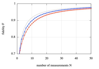
(a) fidelity

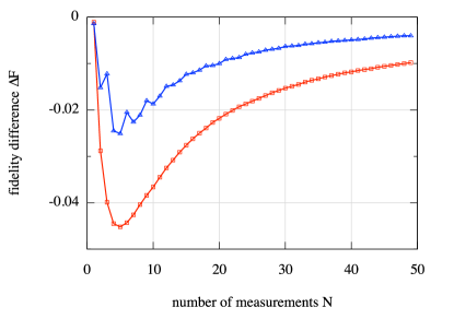
(b) fidelity difference

Figure 1: Least biasedness adaption for qubits. The blue triangles denote least biasedness adaption, using equation (5), compared to random measurements (red squares) and the theoretical maximum (grey line). In (a) the absolute estimation fidelities are shown, whereas (b) depicts the difference $\Delta F=F-F_{\mathrm{opt}}$ between the simulation fidelities $F$ and the optimal fidelity (6).

(a) $d=4$

(b) $d=6$

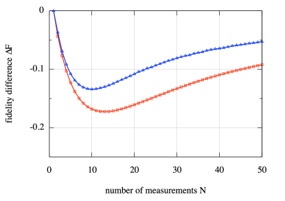
(c) $d=8$

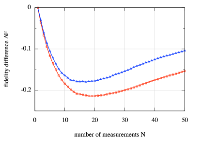
(d) $d=13$

Figure 2: Least biasedness adaption for different dimensions. The fidelity difference $\Delta F=F-F_{\mathrm{opt}}$ to the optimal fidelity (7) is shown for four exemplary dimensions $d$. The blue triangles denote least biasedness adaption compared to random measurements (red squares).

The described method can be used for adaptive estimation of qubits. The result of the corresponding simulations is depicted in figure 1.

The resulting estimation fidelities are close to the theoretical maximum

$$F_{\mathrm{opt}}=\tfrac{N+1}{N+2}$$ (6)

of collective measurements Massar and Popescu (1995); Derka et al. (1998). Furthermore they are in good agreement with results reported in Fischer et al. (2000), although here much simpler methods are used for adaption and estimation.

5.2 Qudits

The real test for the presented methods is their application to higher dimensional states. In figure 2 we show the estimation fidelities for states of dimension four, six, eight and 13.

In all these examples, there is a gain in estimation fidelities due to adaption compared to the non-adaptive procedure. On the other hand, in contrast to the qubit case, there is a significant gap between adaptive single measurements and theoretical maximal fidelity

$$F_{\mathrm{opt}}=\tfrac{N+1}{N+d}$$ (7)

in $d$ dimensions Bruß and Macchiavello (1999).

The case $d=6$ is of particular interest. Since $6$ is not a prime power, there is no known way to construct the seven MUBs necessary for a Wootters-Fields measurement strategy Wootters and Fields (1989). In fact there are only three MUBs known for $d=6$ Brierley and Weigert (2010). But least bias adaption manages to find six measurement bases unbiased with respect to the measured vectors. Again, this does not mean that the measurement bases are mutually unbiased, but that they have an overlap of $\frac{1}{6}$ only with the basis vectors corresponding to the really observed measurement outcomes. Nonetheless the adaption fidelities are the same that would be achieved with six fixed MUBs. For the seventh and all following measurements the adapted bases are no longer “unbiased” but have only least bias with respect to the previously measured states.

6 Conclusions

We have shown that simple adaptive measurement methods can be successfully applied to higher dimensional quantum states. We presented a method for estimating and adapting in higher dimensions which reconciles the concepts of adaption by information entropy maximisation and mutually unbiased bases.

The simulated estimation fidelities using these methods, although smaller than the theoretical maximum, show a clear fidelity gain of up to $5\%$ compared to non-adaptive methods. This is independent of the dimension and therefore also works for dimensions for which no full set of mutually unbiased bases is known.

References

- Paris and Řeháček (2004) M. G. A. Paris and J. Řeháček, eds., Quantum State Estimation (Springer, Berlin, 2004).
- Raymer (1997) M. G. Raymer, Contemporary Physics, 38, 343 (1997).
- Dieks (1982) D. Dieks, Phys. Lett. A, 92, 271 (1982).
- Wootters and Zurek (1982) W. K. Wootters and W. Zurek, Nature, 299, 802 (1982).
- Massar and Popescu (1995) S. Massar and S. Popescu, Phys. Rev. Lett., 74, 1259 (1995).
- Derka et al. (1998) R. Derka, V. Bužek, and A. K. Ekert, Phys. Rev. Lett., 80, 1571 (1998).
- Bruß and Macchiavello (1999) D. Bruß and C. Macchiavello, Phys. Lett. A, 253, 249 (1999).
- Hradil et al. (2000) Z. Hradil, J. Řeháček, G. Badurek, and H. Rauch, Phys. Rev. A, 62, 014101 (2000).
- Bagan et al. (2002) E. Bagan, M. Baig, and R. Muñoz-Tapia, Phys. Rev. Lett., 89, 277904 (2002).
- Bagan et al. (2005) E. Bagan, A. Monras, and R. Muñoz-Tapia, Phys. Rev. A, 71, 062318 (2005).
- Bagan et al. (2006) E. Bagan, M. A. Ballester, R. D. Gill, A. Monras, and R. Muñoz-Tapia, Phys. Rev. A, 73, 032301 (2006).
- Fischer et al. (2000) D. G. Fischer, S. H. Kienle, and M. Freyberger, Phys. Rev. A, 61, 032306 (2000).
- Hradil (1997) Z. Hradil, Phys. Rev. A, 55, R1561 (1997).
- Wootters and Fields (1989) W. K. Wootters and B. D. Fields, Ann. Phys. (N.Y.), 191, 363 (1989).
- Klimov et al. (2008) A. B. Klimov, C. Muñoz, A. Fernández, and C. Saavedra, Phys. Rev. A, 77, 060303 (2008).
- Adamson and Steinberg (2010) R. B. A. Adamson and A. M. Steinberg, Phys. Rev. Lett., 105, 030406 (2010).
- Lima et al. (2011) G. Lima, L. Neves, R. Guzmán, E. S. Gómez, W. A. T. Nogueira, A. Delgado, A. Vargas, and C. Saavedra, Opt. Express, 19, 3542 (2011), arXiv:1003.2125 [quant-ph] .
- Hioe and Eberly (1981) F. T. Hioe and J. H. Eberly, Phys. Rev. Lett., 47, 838 (1981).
- Mahler and Weberruß (1995) G. Mahler and V. A. Weberruß, Quantum Networks (Springer, Berlin, 1995).
- Bschorr et al. (2006) T. C. Bschorr, S. Probst-Schendzielorz, and M. Freyberger, Eur. Phys. J. D, 37, 141 (2006).
- Happ and Freyberger (2008) C. J. Happ and M. Freyberger, Phys. Rev. A, 78, 064303 (2008).
- Durt et al. (2010) T. Durt, B.-G. Englert, I. Bengtsson, and K. Życzkowski, Int. J. Quatum Information, 8, 535 (2010), arXiv:1004.3348 [quant-ph] .
- Nielsen and Chuang (2000) M. A. Nielsen and I. L. Chuang, Quantum Computation and Quantum Information (Cambridge University Press, Cambridge, 2000).
- Cover and Thomas (2006) T. M. Cover and J. A. Thomas, Elements of Information Theory (Wiley, Hoboken, 2006).
- Hurwitz (1897) A. Hurwitz, Nachrichten von der königlichen Gesellschaft der Wissenschaften zu Göttingen, Mathematisch-physikalische Klasse, 1897, 71 (1897).
- Życzkowski and Kuś (1994) K. Życzkowski and M. Kuś, J. Phys. A: Math. Gen., 27, 4235 (1994).
- Brierley and Weigert (2010) S. Brierley and S. Weigert, J. Phys.: Conf. Ser., 254, 012008 (2010), arXiv:1006.0093 [quant-ph] .