Subtraction of the spurious translational mode from the RPA response function

Abstract

It is well known that within self-consistent Random Phase Approximation (RPA) on top of Hartree-Fock (HF), the translational symmetry should be restored. Due to approximations at the level of the practical implementation, this restoration may be only partial. As a result, one has spurious contributions in the physical quantities that are extracted from RPA. While there are several recipes in the literature to overcome this drawback in order to produce transition densites or strength functions that are free from spurious contamination, there is no formalism associated with the full RPA response function. We present such formalism in this paper. Our goal is to avoid spurious contamination when the response function is used in many-body frameworks like the particle-vibration coupling theory.

I Introduction

RPA is one of the basic tools to study the nuclear vibrational excitations. The basic theory is well known, and several versions have been implemented since the early days of nuclear structure studies. However, while in the past the underlying mean field and the residual particle-hole (p-h) interactions were often purely empirical, nowadays self-consistent HF plus RPA calculations are feasible with quite sophisticated effective forces. The importance of these calculations stems from the possibility of testing their predictive power, e.g., when going towards neutron-rich (or neutron-deficient) isotopes that can be studied at present or future radioactive beam facilities.

One of the advantages of RPA is that it is a conserving theory, that is, the symmetries of the Hamiltonian that are broken at the HF level are in principle restored in RPA. The detailed way in which this restoration is realized has been already widely discussed in the literature. The reader can consult standard textbooks (cf. Refs. Ring-Schuck ; Blaizot-Ripka ) or review papers like Ref. Lane . The purpose of the present work is not to re-discuss basic questions. We shall focus instead on practical issues, in the case of the restoration of translational symmetry (which is associated with the appearance of a zero-energy translational mode in the RPA $J^{\pi}=1^{-}$ spectrum).

In practice, it is impossible to obtain this translational mode at exactly zero energy due to some theoretical or numerical approximation. If we restrict ourselves to the case of nonrelativistic calculations performed with effective Skyrme forces, no fully self-consistent calculations that treat the continuum exactly are available. Fully self-consistent calculations in which the continuum is discretized do exist Terasaki1 ; Colo2 , and in this case the energy of the spurious translational mode goes to zero as the dimension of the box in which the system is set increases. Both in this case, and in the case of continuum calculations which are the object of our study, one has then to deal with the spurious contamination of several quantities.

In fact, if the spurious state from a numerical calculation does not lie at zero energy, and its wavefunction does not coincide with the true translational wavefunction, the other (physical) states contain some admixture of the ideal spurious state. These admixtures should be eliminated. Various procedures have been proposed, depending on the specific RPA implementation. In the case of coordinate-space RPA the basic question is how to remove spurious admixtures from the strength function associated with a given operator $\hat{F}({\bf r})$ acting in the 1^- channel, namely from

$$S(E)=\sum_{n}|\langle n|\hat{F}|\tilde{0}\rangle|^{2}\delta(E-E_{n}),$$ (1)

where we suppose that $|n\rangle$ are the RPA states having respectively energy $E_{n}$ and $|\tilde{0}\rangle$ is the nuclear ground-state. We assume that the definition can be formally extended to the continuum case, when the spectrum is not discrete. Sometimes one is willing to remove the spurious admixtures directly from the transition densities, that are defined as

$$\delta\rho_{n}({\bf r})=\langle n|\hat{\rho}({\bf r})|\tilde{0}\rangle,$$ (2)

where $\hat{\rho}$ is the density operator. Once more, this definition holds if the spectrum is continuum and the transition density is associated with a state at every positive energy $\omega$: we will use the notation $\delta\rho(\mbox{\boldmath$r$}\omega)$ in what follows.

These two problems have been dealt with extensively in the literature (see Refs. Giai1 ; Suzuki ; Sagawa ; Colo1 ; Hamamoto ; Shlomo1 ; Terasaki1 ). The solutions include projection methods, use of corrected effective operators etc. However, the present work is motivated by the use of the dipole RPA spectrum not by itself, but as an input to particle-vibration coupling (PVC) calculations BM ; Mahaux ; Colo10 . In PVC calculations performed in coordinate space with proper continuum coupling Mizuyama_tbp the full RPA response function enters; consequently, one must deal with the subtraction of spurious contamination from that quantity. Since this has not been discussed in the literature previously, to our best knowledge, we discuss the problem in the present paper. The next Section deals with the theoretical formalism.

II Method

As recalled in the Introduction, the spurious dipole mode is originated by the restoration of the translational symmetry in RPA. Translations along one direction, say the $z$-axis, are generated by the total momentum operator $\hat{P}$ which is a conserved quantity, i.e., $[H,\hat{P}]=0$. As discussed in Ring-Schuck ; Blaizot-Ripka ; Thouless , the ideal spurious state must have $X$ and $Y$ amplitudes associated with the p-h matrix elements of $\hat{P}$. Because of the symmetry of the RPA matrix, its non-zero eigenvalues and eigenvectors appear in pairs. The partner of the spurious state has amplitudes related to the matrix element of the operator $\hat{Q}$ that satisfies $[H,\hat{Q}]=\frac{-i\hbar}{Am}\hat{P}$. This latter equation is associated with the Galilean invariance as it is shown in Refs. Ring-Schuck ; Blaizot-Ripka .

In this Section, we show a method which removes the spurious contribution from the RPA response function in coordinate space representation. We express the formulas that have been introduced in Ref. Nakatsukasa in coordinate space representation, and extend them to case of the RPA response function.

In order to remove spurious admixtures, first of all, as in Ref. Nakatsukasa , we suppose the validity of

$$\delta\hat{\rho}(\omega)=\delta\hat{\tilde{\rho}}(\omega)+\lambda_{P}(\omega)\delta\hat{\rho}_{P}+\lambda_{Q}(\omega)\delta\hat{\rho}_{Q},$$ (3)

together with the orthogonality conditions $[\delta\hat{\tilde{\rho}}(\omega),\delta\hat{\rho}_{P}]=[\delta\hat{\tilde{\rho}}(\omega),\delta\hat{\rho}_{Q}]=0$, for the “physical” transition density operator $\delta\hat{\tilde{\rho}}(\omega)$ in its second-quantized form. $\delta\hat{\rho}(\omega)$ is the second-quantized form of the RPA transition density operator. $\delta\hat{\rho}_{P}$ and $\delta\hat{\rho}_{Q}$ are related with $\hat{P}$ and $\hat{Q}$ by

$$\delta\hat{\rho}_{P} = i\sum_{q,\sigma}\int d\mbox{\boldmath$r$}\hat{\psi}_{q}^{\dagger}(\mbox{\boldmath$r$}\sigma)(-i\hbar\nabla_{z})\hat{\psi}_{q}(\mbox{\boldmath$r$}\sigma)=i\hat{P},$$ (4)

$$\delta\hat{\rho}_{Q} = i\sum_{q,\sigma}\int d\mbox{\boldmath$r$}\hat{\psi}_{q}^{\dagger}(\mbox{\boldmath$r$}\sigma)z\hat{\psi}_{q}(\mbox{\boldmath$r$}\sigma)=i\hat{Q}.$$ (5)

The canonicity conditions $[\delta\hat{\rho}_{Q},\delta\hat{\rho}_{P}]=-[\hat{Q},\hat{P}]=-i\hbar A$ hold.

The transition density $\delta\rho(\mbox{\boldmath$r$}\omega)$ in coordinate space representation obeys

$$\delta\rho_{q,\alpha}(\mbox{\boldmath$r$}\omega)=\langle 0|[\hat{\rho}_{q,\alpha}(\mbox{\boldmath$r$}),\delta\hat{\rho}(\omega)]|0\rangle,$$ (6)

where $\hat{\rho}_{q,\alpha}(\mbox{\boldmath$r$})$ is the density operator defined by

$$\hat{\rho}_{q,\alpha}(\mbox{\boldmath$r$}) = \sum_{\sigma}\hat{\psi}^{\dagger}_{q}(\mbox{\boldmath$r$}\sigma)\hat{O}_{\alpha}(\mbox{\boldmath$r$})\hat{\psi}_{q}(\mbox{\boldmath$r$}\sigma)$$ (7)

$$\mbox{with }\hat{O}_{\alpha}(\mbox{\boldmath$r$})\in\{1,\overrightarrow{\nabla}\pm\overleftarrow{\nabla},...\}.$$

Using Eq. (3) and Eq. (6), we obtain

$$\delta\rho_{q,\alpha}(\mbox{\boldmath$r$}\omega) = \delta\tilde{\rho}_{q,\alpha}(\mbox{\boldmath$r$}\omega)+\lambda_{P}(\omega)\langle 0|[\hat{\rho}_{q,\alpha}(\mbox{\boldmath$r$}),\delta\hat{\rho}_{P}]|0\rangle$$ (8)

$$+\lambda_{Q}(\omega)\langle 0|[\hat{\rho}_{q,\alpha}(\mbox{\boldmath$r$}),\delta\hat{\rho}_{Q}]|0\rangle.$$

By using Eq. (3) and Eq. (6) with the orthogonality condition and the canonicity condition, $\lambda_{P}(\omega)$ and $\lambda_{Q}(\omega)$ are represented by the transition densities in coordinate space representation as

$$\lambda_{P}(\omega) = \frac{\langle 0|[\delta\hat{\rho}_{Q},\delta\hat{\rho}(\omega)]|0\rangle}{\langle 0|[\delta\hat{\rho}_{Q},\delta\hat{\rho}_{P}]|0\rangle}=\frac{-1}{\hbar A}\sum_{q}\int d\mbox{\boldmath$r$}z\delta\rho_{q}(\mbox{\boldmath$r$}\omega),$$

(9)

$$\lambda_{Q}(\omega) = -\frac{\langle 0|[\delta\hat{\rho}_{P},\delta\hat{\rho}(\omega)]|0\rangle}{\langle 0|[\delta\hat{\rho}_{Q},\delta\hat{\rho}_{P}]|0\rangle}=\frac{1}{A}\sum_{q}\int d\mbox{\boldmath$r$}\delta j_{z,q}(\mbox{\boldmath$r$}\omega).$$

For example, if $\hat{O}_{\alpha}(\mbox{\boldmath$r$})=1$, then Eq. (8) becomes

$$\delta\rho_{q}(\mbox{\boldmath$r$}\omega) = \delta\tilde{\rho}_{q}(\mbox{\boldmath$r$}\omega)$$ (11)

$$+\nabla_{z}\rho_{q}(\mbox{\boldmath$r$})\frac{-1}{A}\sum_{q^{\prime}}\int d\mbox{\boldmath$r$}^{\prime}z^{\prime}\delta\rho_{q^{\prime}}(\mbox{\boldmath$r$}^{\prime}\omega)$$

because $\langle 0|[\hat{\rho}_{q}(\mbox{\boldmath$r$}),\delta\hat{\rho}_{P}]|0\rangle=\hbar\nabla_{z}\rho_{q}(\mbox{\boldmath$r$})$. As a further example, if $\hat{O}_{\alpha}(\mbox{\boldmath$r$})=\overrightarrow{\nabla}-\overleftarrow{\nabla}$, one has

$$\delta 2i\mbox{\boldmath$j$}_{q}(\mbox{\boldmath$r$}\omega) = \delta 2i\tilde{\mbox{\boldmath$j$}}_{q}(\mbox{\boldmath$r$}\omega)$$

$$+\rho_{q}(\mbox{\boldmath$r$})\frac{\hat{e}_{z}}{2A}\sum_{q^{\prime}}\int d\mbox{\boldmath$r$}^{\prime}\delta 2ij_{z,q^{\prime}}(\mbox{\boldmath$r$}^{\prime}\omega)$$

because $\langle 0|[2i\hat{\mbox{\boldmath$j$}}_{q}(\mbox{\boldmath$r$}),\delta\hat{\rho}_{Q}]|0\rangle=i\hat{e}_{z}\rho_{q}(\mbox{\boldmath$r$})$ ($\hat{e}_{z}$ is the unit vector along $z$).

In this paper, we extend the above method to single out “physical” quantities labelled by a tilde, to the case of the response function instead of the transition density. We adopt here the same notation as in Ref. mizuyama . The response function $R^{\alpha\beta}_{qq^{\prime}}$ depends on two indices $\alpha$ and $\beta$ that identify the operators as in Eq. (7).

As in Ref. mizuyama , one can write

$$\delta\rho_{q}(\mbox{\boldmath$r$}\omega) = \sum_{q^{\prime}}\int d\mbox{\boldmath$r$}^{\prime}R^{1,1}_{qq^{\prime}}(\mbox{\boldmath$r$}\mbox{\boldmath$r$}^{\prime};\omega)f_{q^{\prime}}(\mbox{\boldmath$r$}^{\prime}),$$ (13)

$$\delta 2i\mbox{\boldmath$j$}_{q}(\mbox{\boldmath$r$}\omega) = \sum_{q^{\prime}}\int d\mbox{\boldmath$r$}^{\prime}R^{\nabla_{-},1}_{qq^{\prime}}(\mbox{\boldmath$r$}\mbox{\boldmath$r$}^{\prime};\omega)f_{q^{\prime}}(\mbox{\boldmath$r$}^{\prime}),$$ (14)

where $f(\mbox{\boldmath$r$})$ is the external operator. In the previous formula the superscript 1 refers to the identity operator and the superscript $\nabla_{-}$ to the operator $\overrightarrow{\nabla}-\overleftarrow{\nabla}$.

We can use Eqs. (11) and (13); then, for the response function we can arrive at

$$\tilde{R}^{11}_{qq^{\prime}}(\mbox{\boldmath$r$}\mbox{\boldmath$r$}^{\prime};\omega)=R^{11}_{qq^{\prime}}(\mbox{\boldmath$r$}\mbox{\boldmath$r$}^{\prime};\omega)$$

$$-\nabla_{z}\rho_{q}(\mbox{\boldmath$r$})\frac{-1}{A}\sum_{q^{\prime\prime}}\int d\mbox{\boldmath$r$}^{\prime\prime}z^{\prime\prime}R^{11}_{q^{\prime\prime}q^{\prime}}(\mbox{\boldmath$r$}^{\prime\prime}\mbox{\boldmath$r$}^{\prime};\omega).$$ (15)

This is our main result. It allows extracting the “physical” response function $\tilde{R}$ from the RPA result $R$.

In the next Section, we illustrate our method by means of some numerical results for the strength function $S$. In fact, by using the “physical” response function defined in Eq. (15), the “physical” strength function can be written as

$$\tilde{S}(\omega) = -\frac{1}{\pi}\mbox{Im}\sum_{qq^{\prime}}\int\!\!\int\!\!d\mbox{\boldmath$r$}d\mbox{\boldmath$r$}^{\prime}f_{q}^{*}(\mbox{\boldmath$r$})\tilde{R}^{11}_{qq^{\prime}}(\mbox{\boldmath$r$}\mbox{\boldmath$r$}^{\prime};\omega)f_{q^{\prime}}(\mbox{\boldmath$r$}^{\prime})$$ (16)

$$= S(\omega)$$

$$-\frac{1}{\pi}\mbox{Im}\sum_{q}\int\!\!d\mbox{\boldmath$r$}f_{q}^{*}(\mbox{\boldmath$r$})\nabla_{z}\rho_{q}(\mbox{\boldmath$r$})/A$$

$$\times\left[\sum_{q^{\prime}q^{\prime\prime}}\int\!\!d\mbox{\boldmath$r$}^{\prime}\int d\mbox{\boldmath$r$}^{\prime\prime}z^{\prime\prime}R^{11}_{q^{\prime\prime}q^{\prime}}(\mbox{\boldmath$r$}^{\prime\prime}\mbox{\boldmath$r$}^{\prime};\omega)f_{q^{\prime}}(\mbox{\boldmath$r$}^{\prime})\right]$$

$$= S(\omega)-\delta S(\omega),$$

where $S(\omega)$ is the strength function defined by the RPA without corrections and $\delta S(\omega)$ is the spurious contribution.

As mentioned in the Introduction, the main point of correcting the response function instead of the transition densities or transition strength is that the response function is an input for more sophisticated many-body frameworks like the particle-vibration coupling approach. In this case, the static HF potential is generalized to a time-dependent (or energy-dependent) self-energy function. This self-energy function $\Sigma$ is associated with the coupling of single-nucleon states with RPA vibrations; consequently, it can be defined in terms of the HF Green’s function $G_{0}$ and the RPA response function. This definition can be found in the references mentioned in the Introduction. However, we have recently tried for the first time Mizuyama_tbp to formulate this theory in coordinate space. In this case, in order to remove the contribution of the spurious state by using Eq. (15), the self-energy function must be expressed as

$$\tilde{\Sigma}(\mbox{\boldmath$r$}\sigma,\mbox{\boldmath$r$}^{\prime}\sigma^{\prime};\omega)$$

$$=\int_{-\infty}^{\infty}\frac{d\omega^{\prime}}{2\pi}\kappa(\mbox{\boldmath$r$})G_{0}(\mbox{\boldmath$r$}\sigma,\mbox{\boldmath$r$}^{\prime}\sigma^{\prime};\omega-\omega^{\prime})\kappa(\mbox{\boldmath$r$}^{\prime})i\tilde{R}^{11}(\mbox{\boldmath$r$}\mbox{\boldmath$r$}^{\prime};\omega^{\prime}),$$

(17)

where $\kappa$ is the residual (p-h) interaction.

Using this self-energy function, we can solve the Dyson equation $G=G_{0}+G_{0}\tilde{\Sigma}G$ in coordinate space, and then obtain the perturbed Green’s function. The detail of the formulas will be in our forthcoming paper Mizuyama_tbp , where also several results are discussed. In the present work, we present some few results about the relevance of projecting out the spurious contribution.

III Numerical results

In this Section, we study the strength functions both in the case of the electric dipole and the isoscalar compression operators. For this study, the nucleus of choice is ²⁰⁸Pb. The equations are solved in a radial mesh that extends up to 20 fm. The radial step is 0.2 fm. The states up to angular momentum $\ell$=12 are included in the model space. The Skyrme set employed is SLy5 Chabanat . The implementation of the continuum RPA is exactly as in Ref. mizuyama .

Also we apply our method to Hartree-Fock plus particle-vibration coupling. As an example, we show the level density in the case of ²⁴O. We included the RPA electric dipole phonons up to 60 MeV. We discuss the spurious state contribution to the level density, extracted from the Green’s function which is solution of the Dyson equation (in the level density we adopt a smoothing parameter equal to 0.4 MeV).

III.1 E1 excitations

In Fig. 1, we display the strength functions (and the associated energy-weighted sum rules, EWSRs) obtained by using the following E1 operators:

$$F_{E1}=e\sum_{p=1}^{Z}r_{p}Y_{1M}(\hat{\mbox{\boldmath$r$}}_{p}),$$ (18)

and

$$\tilde{F}_{E1}=e\sum_{n=1}^{N}\frac{Z}{A}r_{n}Y_{1M}(\hat{\mbox{\boldmath$r$}}_{n})-e\sum_{p=1}^{Z}\frac{N}{A}r_{p}Y_{1M}(\hat{\mbox{\boldmath$r$}}_{p}).$$ (19)

The operator defined by Eq. (19) is obtained by removing the center of mass from the original operator of Eq. (18). We apply our method to obtain $\tilde{S}(\omega)$, by leaving the operator equal to (18), and we obtain the blue curve in Fig. 1. One can compare this result to the E1 spectrum without the spurious subtraction (red curve), and to the one obtained by using the original RPA response and the operator (19) (green curve). In the lower panel of the figure we show the running, or cumulated, values of EWSRs. From both panels one can argue that our method succeeds to remove the spurious state. In particular, the success of our microscopic implementation is very clear from the detailed strength of the upper panel, as no strength remains in the low-energy region down to zero.

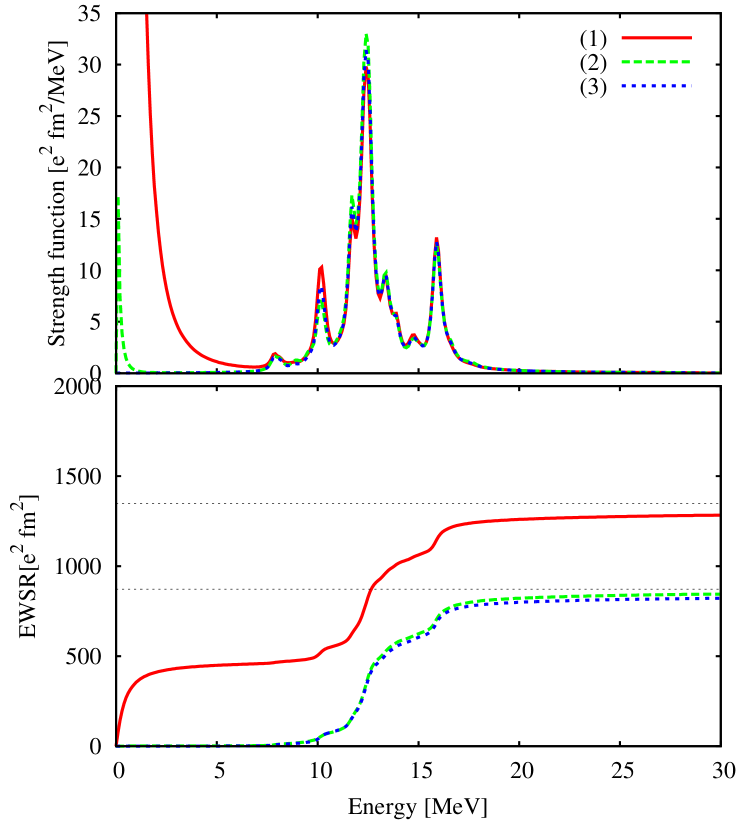
Figure 1: (Color online) The Skyrme continuum RPA results for the E1 strength of ²⁰⁸Pb with the SLy5 Skyrme interaction are displayed in the upper panel. The red curve [labelled by (1) in the figure] is calculated by using the E1 operator (18), whereas the green curve (2) is calculated by using the E1 operator with the center-of-mass subtracted [Eq. (19)], and the blue curve (3) is calculated by using the operator of Eq. (18) but at the same time with the spurious state eliminated from the response function by using our method. In the lower pannel we show the running (or cumulated) values of the energy weighted sum rules. The dotted lines are the double-commutator values of the energy-weighted sum rules for the operators (18) and (19). The formulas are given in the Appendix [Eqs. (26) and (30), respectively] and the values are shown in Table 1.

III.2 IS compression dipole

Similar accurate results can be obtained if the IS dipole compression operator is applied. This operator reads

$$F_{IS1}=\sum_{i=1}^{A}r^{3}_{i}Y_{1M}(\hat{\mbox{\boldmath$r$}}_{i})$$ (20)

without any center-or-mass subtraction. Many authors have used, to take care of this subtraction, the hydrodynamical ansatz that has been originally proposed in Ref. Giai1 . This amounts to using the operator

$$\tilde{F}_{IS1}=\sum_{i=1}^{A}\left(r^{3}_{i}-\frac{5}{3}\langle r^{2}\rangle r_{i}\right)Y_{1M}(\hat{\mbox{\boldmath$r$}}_{i}),$$ (21)

the factor $5\langle r^{2}\rangle/3$ being often denoted with the symbol $\eta$.

We present our results in a form which is analogous to the one of the previous subsection in Fig. 2. The blue line corresponds to the choice of the bare operator (20), and to the miscroscopic subtraction of the center-of-mass motion proposed in our present work. The associated result can be compared with the use of the operator (21) in connection with the original RPA response (green curve) and to the RPA result without any subtraction of the center-of-mass either in the operator or in the response function (red curve).

The result of the red curve includes the spurious contributions. Both other curves provide a way to remove these contributions. Although similar, they are not identical: in this respect, the upper panel of Fig. 2 shows to which extent the ansatz (21) for the effective operator is accurate. The small differences are not visible if one looks only at the cumulated EWSRs: both the blue and green line converge to the same result.

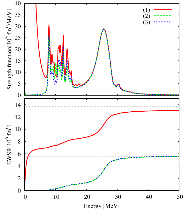
Figure 2: (Color online) Same as Fig.1 for the isoscalar compression dipole spectrum. The nucleus is ²⁰⁸Pb and the Skyrme set is SLy5. The red curve [labelled by (1) in the figure] is calculated by using the operator (20), whereas the green curve (2) is calculated by using the operator with the center-of-mass subtracted [Eq. (21)], and the blue curve (3) is calculated by using the operator Eq. (20) but at the same time with the spurious state eliminated from the response function by using our method. In the lower pannel we show the running (or cumulated) values of the energy weighted sum rules. The dotted lines are the double-commutator values of the energy-weighted sum rules for the operators (20) and (21). The formulas are given in the Appendix and the values are shown in Table 1.

	Operator	$\tilde{m_{1}}$	$m_{1}$	$\delta m_{1}$
E1	(18)	872.3	1350	477.7
	(19)	872.3	872.3	0.0
Compression dip.	(20)	$5.588\times 10^{6}$	$1.368\times 10^{7}$	$8.092\times 10^{6}$
	(21)	$5.588\times 10^{6}$	$5.588\times 10^{6}$	0.0

Table 1: Values of the energy-weighted sum rule for the E1 and the isoscalar compression dipole excitations in ²⁰⁸Pb with SLy5. These values correspond to the dotted lines in Fig. 1 and 2. $\delta m_{1}$ is the contribution arising from the center-of-mass spurious motion. Definition are given in the Appendix: in particular $\tilde{m}_{1}$ is defined by Eq. (24).

III.3 Spurious mode subtraction in PVC

The level density $\rho_{lj}$ can be defined as

$$\rho_{lj}(\omega)=\frac{\pm 1}{\pi}\int_{0}^{\infty}dr\mbox{Im}G_{lj}(rr,\omega),$$ (22)

where $G_{lj}$ can be either the Hartree-Fock Green’s function or the perturbed Green’s function which is obtained by solving the Dyson equation. The spurious state may affect the self-energy function that appears in the Dyson equation because the definition includes the RPA response function. Therefore, the spurious contribution should be systematically eliminated from the response function.

In the neutron-rich nuclei like ²⁴O, low-lying E1 strength can be larger than in other systems, and the spurious state is not well separated from the other physical states, as it is shown in Fig. 3.

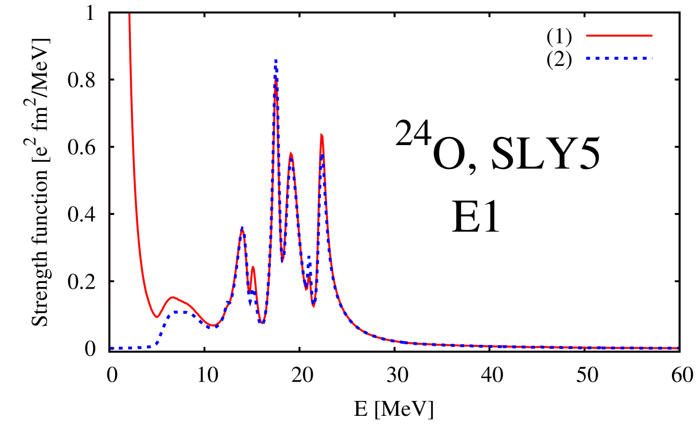
Figure 3: (Color online) Same as Fig. 1 for ²⁴O. The solid red curve [labelled by (1) in the figure] is calculated by using the operator (18), and the dotted blue curve (2) is calculated by using the operator Eq. (18) but at the same time with the spurious state eliminated from the response function by using our method.

In Fig.4, the level density is plotted as a function of the single particle energy. The dotted black curve is the Hartree-Fock level density. The solid red curve is the HF+PVC level density, in which the spurious contribution is properly removed. The dashed blue curve is the HF+PVC level density, but when the spurious state is not removed. We have studied neutron level densities, and in particular the upper pannel is the level density in the $(p_{3/2})^{-1}$ case, and the lower pannel is the $(s_{1/2})^{-1}$ case. By comparing the solid red curve and the dashed blue curve, we can see that the unphysical contribution of the spurious state cannot be ignored.

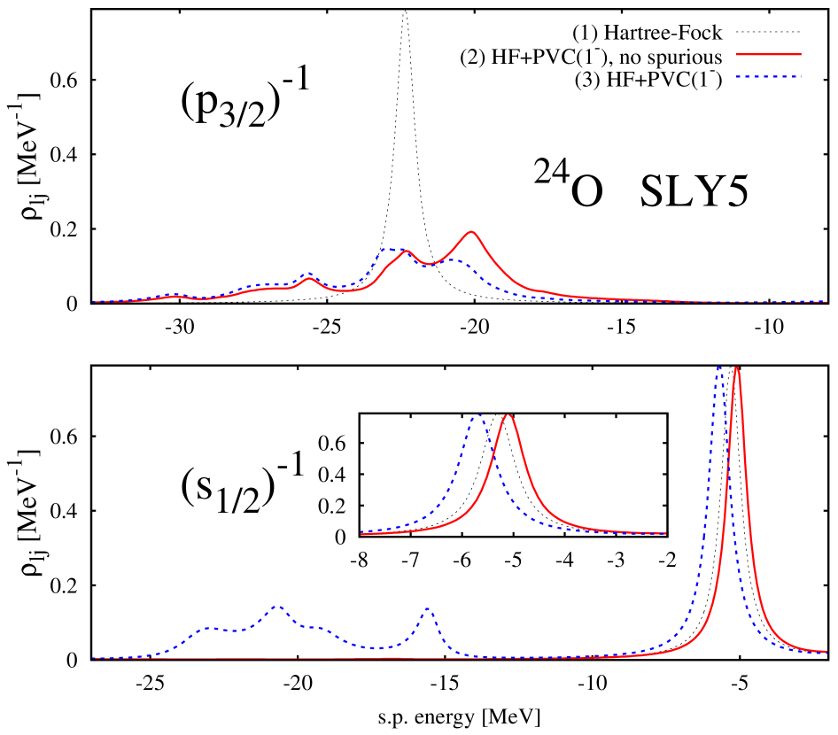
Figure 4: (Color online) The level density defined by Eq. (22) in ²⁴O. The dotted black curve [labelled by (1) in the figure] is the Hartree-Fock level density. The solid red curve [labelled by (2) in the figure] is the HF+PVC level density when the spurious state is removed by applying Eq. (15). The dashed blue curve [labelled by (3) in the figure] is also the HF+PVC level density, but when the spurious state is not removed. The upper panel corresponds to $(p_{3/2})^{-1}$, and the lower panel is $(s_{1/2})^{-1}$ orbit.

IV Summary

While RPA provides, in principle, a theoretical framework that restores the symmetries which are broken at the mean field level, approximations that are often made can spoil this feature. This is particularly true for the case of the translational symmetry. It has been known for several decades that the self-consistency violations, the cutoff in the model space and/or other limitations of the practical RPA implementations leave the spurious center-of-mass motion at finite instead of zero energy and give associated contaminations of the wavefunctions and physical observables related with the RPA states.

Many papers have been devoted to this problem, yet the subject of this work is the removal of spurious contributions from the RPA full response function, within the continuum RPA on top of Skyrme HF framework. We have presented a microscopic formalism that is claimed to be able to achieve this removal quite successfully, and we have validated this statement by means of accurate calculations of the E1 and isoscalar compression spectra of ²⁰⁸Pb.

The original motivation of this work is the possibility of using the RPA response function for particle-vibration coupling calculations. Indeed we have shown, by using the example of level densities in ²⁴O, that the results of PVC either with or without the proper subtraction of the spurious state can substantially differ. Other many-body scheme or reaction calculations require the use of the response function. In all these cases, our proposed method can display its usefulness.

Appendix A Energy-weighted sum rules of interest

In general, we define the energy-weighted sum rule associated with the strength function $S(\omega)$ as

$$m_{1}=\int d\omega\omega S(\omega).$$ (23)

Consistently with Eq. (16) we define

$$\tilde{m}_{1}=\int d\omega\omega\tilde{S}(\omega)=m_{1}-\delta m_{1}$$ (24)

with

$$\delta m_{1}=\int d\omega\omega\delta S(\omega).$$ (25)

It is well known that $m_{1}$ can be calculated analitically by means of the expectation value of the double commutator. In this Appendix, we only summarize the useful results in the case of Skyrme interactions.

A.1 The E1 operator

The $m_{1}$ associated with the operator (18) is given by

$$m_{1}=\frac{e^{2}\hbar^{2}}{2m}\frac{9}{4\pi}Z+\frac{9}{4\pi}e^{2}bI,$$ (26)

with

$$b = \frac{1}{4}\left(t_{1}(1+\frac{1}{2}x_{1})+t_{2}(1+\frac{1}{2}x_{2})\right),$$ (27)

$$I = \int dr4\pi r^{2}\rho_{n}(r)\rho_{p}(r).$$ (28)

The second term of $m_{1}$ is a correction arising from the momentum-dependent terms of the Skyrme interaction.

$\delta m_{1}$ is given by

$$\delta m_{1}=\frac{e^{2}\hbar^{2}}{2m}\frac{9}{4\pi}\frac{Z^{2}}{A}.$$ (29)

Therefore,

$$\tilde{m}_{1} = m_{1}-\delta m_{1}$$ (30)

$$= \frac{e^{2}\hbar^{2}}{2m}\frac{9}{4\pi}Z+\frac{9}{4\pi}e^{2}bI-\frac{e^{2}\hbar^{2}}{2m}\frac{9}{4\pi}\frac{Z^{2}}{A}$$

$$= \frac{e^{2}\hbar^{2}}{2m}\frac{9}{4\pi}\frac{NZ}{A}+\frac{9}{4\pi}e^{2}bI.$$

The $m_{1}$ associated with the operator (19) is given by terasaki ; Shlomo2

$$m_{1}=\frac{e^{2}\hbar^{2}}{2m}\frac{9}{4\pi}\frac{NZ}{A}+\frac{9}{4\pi}e^{2}bI,$$ (31)

and, as expected, Eq. (30) and (31) are completely equivalent.

A.2 The compression dipole operator

The $m_{1}$ with the operator (20) is given by

$$m_{1}=\frac{\hbar^{2}}{2m}\frac{3}{4\pi}A\langle 11r^{4}\rangle.$$ (32)

Also $\delta m_{1}$ can be derived easily as

$$\delta m_{1}=\frac{\hbar^{2}}{2m}A\frac{1}{4\pi}\langle 5r^{2}\rangle\langle 5r^{2}\rangle,$$ (33)

and therefore

$$\tilde{m}_{1} = m_{1}-\delta m_{1}$$ (34)

$$= \frac{\hbar^{2}}{2m}\frac{3}{4\pi}A\langle 11r^{4}\rangle-\frac{\hbar^{2}}{2m}\frac{1}{4\pi}A\langle 5r^{2}\rangle^{2}$$

$$= \frac{\hbar^{2}}{2m}\frac{1}{4\pi}A\left(33\langle r^{4}\rangle-25\langle r^{2}\rangle^{2}\right).$$

On the other hand, the energy-weighted sum rule $m_{1}$ associated with (21) reads

$$m_{1}=\frac{\hbar^{2}}{2m}\frac{1}{4\pi}A\left(33\langle r^{4}\rangle-25\langle r^{2}\rangle^{2}\right).$$ (35)

Once more, Eq. (34) and (35) are completely equivalent.

References

• (1) P. Ring, P. Schuck, The Nuclear Many-Body Problem (Springer-Verlag, Berlin, 1980).
• (2) J. -P. Blaizot  and  G. Ripka, Quantum Theory of Finite Systems (The MIT Press, Cambridge, 1986).
• (3) A. M. Lane, J. Martorell, Ann. Phys. 129, 273 (1980).
• (4) J. Terasaki, J. Engel, M. Bender, J. Dobaczewski, W. Nazarewicz, and M. Stoitsov, Phys. Rev. C71, 034310 (2005).
• (5) G. Colò, P. F. Bortignon, S. Fracasso and N. Van Giai, Nucl. Phys. A788 (2007) 173c; G. Colò, L. Cao, N. Van Giai, L. Capelli, Comp. Phys. Comm. (submitted).
• (6) N. Van Giai, H. Sagawa, Nucl. Phys. A371, 1 (1981).
• (7) F. E. Serr, T. S. Dumitrescu,  Toru Suzuki  and C. H. Dasso, Nucl. Phys. A404, 359 (1983).
• (8) I. Hamamoto  and  H. Sagawa,  Phys. Rev. C 48, R960 (1993).
• (9) G. Colò, N. Van Giai, P. F. Bortignon, M. R. Quaglia,  Phys. Lett. B485, 362 (2000).
• (10) I. Hamamoto, H. Sagawa, Phys. Rev. C66, 044315 (2002).
• (11) B. K. Agrawal, S. Shlomo, A. I. Sanzhur, Phys. Rev. C67, 034314 (2003).
• (12) A. Bohr, B. R. Mottelson, Nuclear Structure. Vol. II (W.A. Benjamnin, New York, 1975).
• (13) C. Mahaux, P. F. Bortignon, R. A. Broglia, and C. H. Dasso, Phys. Rep. 120, 1 (1985).
• (14) G. Colò, H. Sagawa, and P. F. Bortignon, Phys. Rev. C82, 064307 (2010).
• (15) K. Mizuyama, G. Colò, E. Vigezzi (to be published).
• (16) D. J. Thouless, Nucl. Phys. A22, 78 (1961).
• (17) Takashi Nakatsukasa, Tsunenori Inakura,  and Kazuhiro Yabana, Phys. Rev. C76, 024318 (2007).
• (18) Kazuhito Mizuyama, Masayuki Matsuo, and Yasuyoshi Serizawa, Phys. Rev. C79, 024313 (2009).
• (19) E. Chabanat, P. Bonche, P. Haensel, J. Meyer and R. Schaeffer, Nucl. Phys. A643, 441 (1998).
• (20) J. Terasaki and J. Engel,  Phys. Rev. C74, 044301 (2006).
• (21) Tapas  Sil,  S.  Shlomo,  B.  K.  Agrawal,  and  P. -G.  Reinhard,  Phys. Rev  C73, 034316 (2006).